A BRIEF ASIDE

This review touches on a number of complex mathematical concepts. We have tried as much as possible to avoid mathematical and statistical jargon, kept equations to a minimum, and presented them in an intuitive form, rather than using formal mathematical notations. However, there is no avoiding the underpinnings of the concepts themselves: no matter how the outputs of the spatial analysis work are obtained, whether using off-the-shelf software, with manual or automated procedure, by oneself or commissioned, it is necessary to interpret the outputs. No software can answer the question: what does this output mean in practical terms for my problem? That is however what the health professionals must ultimately do: use the outputs to address problems in a practical way. The interpretation of the output, and the way it is used for follow-up work, be it the collection of more data, the implementation of policies, the establishment of a data analysis facility or of an on-line data portal, the logistics of hospitals or schools, requires that the end-user (the medical provider or health professional, in this case) understands at least intuitively how the output was obtained, and the level of uncertainty associated to the output. Essentially, the ‘black-box’ should be related to the ‘mechanical’ operations carried out to achieve the input, not to the necessary logical steps. We prepared this review with this approach in mind: to walk readers through the logical steps, and to link the steps with the appropriate software (keeping it to broadly available commercial or open-source packages), algorithm or procedure, and some published examples of how the procedures were used, what outputs were obtained, and how these were interpreted.

We will assume here that readers are familiar with at least a working definition of the concepts of variable, space, probability, mean, function, error, data, population, sample, coordinates, algorithm, script. Beyond these, we will provide brief intuitive definitions of the parameters and procedures that we introduce in the review, and as much as possible we will try and link new concepts to the fundamental ones, without delving into details that may detract from this logical flow. This has not been possible in every instance: in the context of a review paper we do not have the scope to present information as we would in a textbook, nor is the purpose of this review scholastic. However, wherever possible, we tried to provide an empirical explanation of concepts and procedures, using examples and illustrations, hoping to encourage the readers to try the procedures themselves, and thus familiarize themselves with the details in practice: essentially, learning by doing. A common criticism of the explosion of statistical and mathematical software materialized in the past few years, is in relation to the ‘black-box’ effect. We agree this is a problem. However, there is an opportunity here. The user-friendliness of spatial analysis functionality of many commercial and open source GIS (e.g. ArcGIS, Quantum GIS) and statistical and programming packages (e.g. R, Python) with a graphical user interface (GUI) and extensive sub-routine libraries, have largely removed the obstacle of needing to learn specific programming languages to carry out data exploration and statistical procedures on large datasets. This has enabled more people in all disciplines to apply mathematical and statistical analysis to their data, and to figure out intuitively, by examination of the outputs, the theoretical concepts underpinning the procedures. Hence we hope that the information contained in this review encourages the readers to try out the software and learn by using it. Table 1 lists some of the most common software used for disease mapping, statistical and spatial analysis. The list is not meant to be exhaustive. Entries are listed in the order they are cited in this review.

Table 1.

List of some widely used commercial and free mapping, statistical, and spatial analysis software

^a Contributors to open source projects and host institutions are fully listed in the software web-portals.

^b Based on information published on the relevant websites.

^c Training required. The level of difficulty is only an indicative estimate: it will depend also on user prior experience with (other) professional software.

^d OSGeo: Open Source Geospatial Foundation. PSF: Python Software Foundation. BUGS: Bayesian inference Using Gibbs Sampling, MRC Biostatistics Unit, Cambridge, UK. GeoBUGS is an add-on to WinBUGS, developed by: Department of Epidemiology and Public Health, Imperial College, St Mary's Hospital, London. CRAN-R project: Comprehensive R Archive Network; CARBayes is authored and maintained by Duncan Lee, Glasgow University, UK. PAHO: Pan America Health Organization – Area of Health Analysis and Information Systems; WHO: World Health Organization.

^e High difficulty may be associated to the need to compile scripts for specific tasks, extensive data processing, or iterations. Prior knowledge of model-based statistics is assumed for WinBUGS, GeoBUGS, CARBayes and SaTScan™.

^f With Information Management Services Inc.

With increasing numbers of users comes also a proliferation of algorithms written for specific applications in specific disciplines. From a purely practical viewpoint this represents another great opportunity, because most algorithms are transferable to other applications. However, this introduces the need for caution: (a) transferability requires a deeper understanding of the computational steps comprised in the algorithms, and it should not be attempted otherwise; (b) the application of concepts may become blurred, and terminology may be applied less rigorously than the original mathematical statements from which the concepts originated; (c) mathematical procedures requiring strong conditions may be applied to datasets or experimental settings lacking those conditions.

A deeper issue relates to the linked concepts of ‘model’ and ‘prediction’, the latter being the ultimate aim of data analysis (in any context). A mathematical model provides a description of a system using mathematical concepts and language. In the realm of statistics an error term is added to the mathematical function:

(1) $${\rm Outcome} = ({\rm Model}) + {\rm Error}$$

(Field et al. Reference Field, Miles and Field2012). The highest form of models is represented by those that provide explanations about the outcome, in other words, those that imply or uncover a causality relationship between the independent variables feeding the model, and the dependent variables in the outcome. These models have true predictive power, because they can be extrapolated to fields or data beyond those used in the original problem, and the independent and dependent variables can be more specifically referred to as: explanatory (or predictor) variables, and explained variables, respectively. The words ‘model’ and ‘prediction’, however, can be also more loosely employed, and usually are, especially in spatial analysis. The form in which [equation 1] is written represents the generic relationship between outcome and model, and in case of empirically determined (i.e. measured) values, holds also in the absence of any associated explanation of causality. In this case the predictive capacity of the model applies only to those objects in the studied set for which data were not collected (i.e. unsampled objects), but whose dependent variable values can be calculated using the model function derived from the measured objects. In spatial analysis this happens every time statistical surfaces are calculated by interpolation between measured points. ‘Prediction’ in this case applies to the use of the model function to derive the values of the variable of interest at locations where the variable was not measured. It is obviously a completely different meaning than, for example, predicting the outbreak of a disease at some time in the future, which can only be done if there is an explanatory relationship between model and outcome. In the epidemiology and parasitology literature both meanings of the term ‘prediction’ are found, sometimes in the same papers. This needs not generate confusion if the relationship between outcome and model is considered by its generic form as given in [equation 1]. The philosophical distinction explained above is fundamental, but for most practical purposes the meanings are clear. For example, when mapping the topography of a geographic area, it is common to take measurements of elevation (variable: z) at some locations indicated by their geographic coordinates (variables: x, y), and then to interpolate the elevation values in between using a mathematical function. Additional functions may be used to smooth the results of the interpolation, if too noisy. Regardless of the functions or numbers of steps performed to derive a digital elevation model, it is clear that z varies (continually) depending on location. But it is equally obvious that there is no relationship of causality between the geographic coordinates and the values of elevation: what we have is just an observed dependency which allows us to predict the data values of elevation at un-measured locations. (The million-year time-scale and plate-size space-scale of geodynamic processes which frame the explanation for the dependency of elevation from geographic coordinates are excluded here.) A completely different matter is to consider the dependence of temperature from elevation. Principles of atmospheric physics provide an explanatory model based on knowledge of the mechanism by which the air temperature changes with elevation, and therefore we not only can interpolate between locations where temperature data were collected, but also extrapolate in space and in time. Henceforward in this paper we will use the words ‘model’ and ‘prediction’ in both senses, trusting the meaning to be clear from the context. In this way we avoid the need for the mathematical proofs of the concepts expressed in this review. We believe this will make the paper more easily readable for a non-specialist audience.

SPATIAL ANALYSIS AND MODELLING

The principal objectives of spatial analysis in the medical context are: (1) to identify disease clusters; (2) to explain the spatial distribution of the clusters; and (3) to predict the risk of disease. These objectives are achieved by visualization, exploration and modelling of data (Pfeiffer et al. Reference Pfeiffer, Robinson, Stevenson, Stevens, Rogers and Clements2008). For this purpose, data files containing geographic references, most commonly expressed as geographic coordinates or area units (e.g. post-codes, school districts, etc.) for each record, are input and organized in a relational geodatabase (RGDB), from which data can be queried and extracted. The first step is to map the data. This allows visualization of any existing spatial patterns, and aids in formulating hypotheses for further analysis. During the analysis stage, the data and their spatial distributions are explored using geostatistical methods, with the purpose of identifying clusters. The explanatory stage of the analysis is aimed at discovering the cause–effect relationships of the distribution and extent of the clusters, leading to predictions. This final stage may require the use of additional layers of information (for example, environmental datasets), and it involves the use of models.

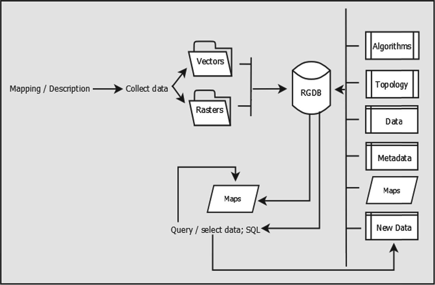
Most off-the-shelf GIS packages presently available provide intuitive tools for visualization and exploration of data. These tools, often available through intuitive GUI, can be effectively applied for processing spatial data also by users not directly familiar with the theoretical underpinnings of the algorithms. So long as the data, including geographic coordinates, are collected and entered in a relational database, the standard functionality of off-the-shelf commercial software can be used to perform preliminary descriptive spatial analysis (Duncombe et al. Reference Duncombe, Clements, Hu, Weinstein, Ritchie and Espino2012). For most purposes this level of data processing is sufficient and may reveal important information for public health professionals. Figure 1 illustrates a possible GIS database architecture for data visualization and mapping, which is generally easy to establish using any of the off-the-shelf mapping packages. Modelling requires in-depth mathematical knowledge and is usually not carried out solely in a GIS environment. It must be emphasized, though, that modern-day challenges in epidemiology and parasitology require the ability to explain and predict the clustering of diseases. In the following section of this review we present a very brief treatment of this topic, in order to provide readers with: (a) basic jargon; and (b) an elementary understanding of how models work and can be interpreted. A review of spatial analysis functionality available from commercial or open source software can be found in De Smith et al. (Reference De Smith, Goodchild and Longley2013), to which we refer the reader also for the theoretical framework underpinning the algorithms.

Fig. 1.

Data and outputs architecture for visualization and mapping. The central element in the system is the relational geodatabase (RGDB), which hosts and organizes the data and the algorithms (including projection algorithms and topology rules) for data processing. Data comprise tables, vector files (points, lines or polygons, collectively defined shapefiles), raster datasets (grids), and metadata, and can be grouped in folders or personal geodatabases of limited capacity. New data are stored and organized in the RGDB. All elements contained in the database can then subsequently be ‘called’ and queried (SQL: Structured Query Language) using the mapping software (algorithms), also stored in the RGDB. Layers, such as shapefiles and rasters can be further elaborated during mapping, and the new products are stored in the database, as well as the maps created.

Central to the correct interpretation of maps and models is an understanding of the nature of uncertainty included in the data. Unfortunately, implementation of routine spatial analysis techniques is not uniform across regions or administrative units, countries, or continents, owing to the scattered nature of data and metadata collected (Brooker et al. Reference Brooker, Katabereine, Gyapong, Stothard and Utzinger2009a ; Brooker, Reference Brooker2010). For example, in preparation of the atlas of human helminth infections in Africa, Brooker et al. (Reference Brooker, Kabatereine, Smith, Mupfasoni, Mwanje, Ndayishimiye, Lwambo, Mbotha, Karanja, Mwandawiro, Muchiri, Clements, Bundy and Snow2009b , Reference Brooker, Hotez and Bundy2010) noted that while some countries (Burundi, Rwanda and Uganda) have comprehensive, country-wide databases of incidence of human infection, others (Kenya and Tanzania) only recorded data from densely populated areas. The problem of spatially varying population sizes (Goovaerts, Reference Goovaerts2005) is not limited to developing countries, but is common also in countries with a long history of geographic data collection, aggregation and archiving. This introduces uncertainty that needs to be dealt with specifically, by the application of more complex analysis and computational procedures, especially when the results of descriptive spatial analysis are used to feed models of risk.

Another source of uncertainty arises from the type of epidemiological data collected. In studies of parasite-induced illness, for example, infection in a community can be measured either by the intensity of infection, i.e. the number of parasites found in each infected host, or by the prevalence of infection, that is, the proportion of infected hosts among all humans examined. Measuring the intensity of infection is resource-intensive and therefore laboratory determinations of the number of parasites in medical specimens from human hosts are most often carried out in cases of advanced morbidity, when patients seek medical assistance, possibly in dedicated structures. Especially for studies aimed at defining the spatial patterns of a disease, prevalence of infection is most often used as a proxy for the occurrence of infections. Prevalence can lead to erroneous interpretations, though, particularly when the population sizes are small or there is uneven distribution of population across regions. In such cases it is difficult to distinguish chance variability from real differences, which may obfuscate the causes of a disease (Sun et al. Reference Sun, Robert, Kim and He2000). On the other hand, the manner of counting for parasites in infected hosts also leads to variability, depending on the techniques and protocols implemented in different laboratories across different geographic areas (Hall and Holland, Reference Hall and Holland2000). Overall, prevalence of infection remains the preferred measure of infection as recommended by the World Health Organization (WHO, 2002), and spatial modelling needs to deal with the related uncertainties.

A source of uncertainty characteristic of the analysis of spatially distributed data and which must be always considered when interpreting spatial variability is known as the ecological fallacy (Piantadosi et al. Reference Piantadosi, Byar and Green1988). This may occur when dealing with the combined use of data of mixed nature, such as point-data (for example, patients, school, etc.) and area data (postal codes), where relationships between variables are inferred to operate at a lower level of disaggregation than the measured variables. These problems require mixed (or multi-level) statistical approaches based on nested units of analysis (Jackson et al. Reference Jackson, Best and Richardson2008; Wakefield, Reference Wakefield2009).

Visualization and exploration

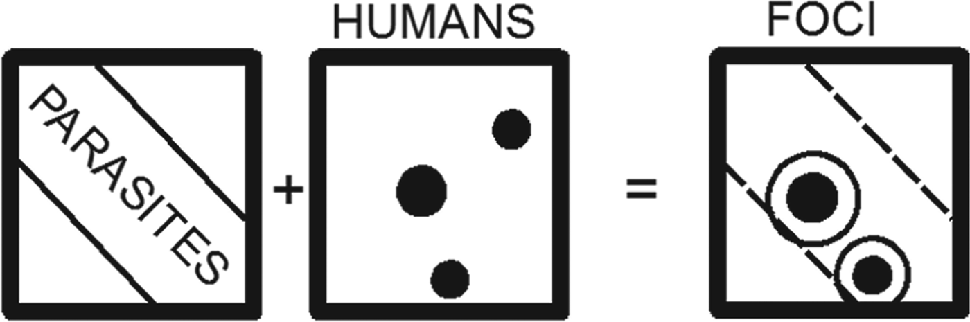
The simplest approach to mapping the distribution of diseases to find their causes and suggest countermeasures to either eliminate them or alleviate their effects is shown in Fig. 2 as an example of parasitic infection of human hosts. This is based on the self-evident concept that only humans exposed to parasites will be infected, and therefore by simple selection of the human cluster locations contained in the area of distribution of parasites it is possible to gain knowledge about where and how to target resources. The addition of other spatially distributed information, such as other factors affecting human health, makes the assessment more complicated by adding new layers of information, but the conceptual approach of selecting areas in which all factors exist at the same time as humans, is the same.

Fig. 2.

Schematic diagram of simple descriptive approach to spatial analysis. The spatial distribution of human clusters (HUMANS) shown as black circles in a x–y (spatial coordinates) plane, overlain to the spatial distribution of parasites (PARASITES) shown as a broad diagonal area in the same x–y plane, results in the selection of human clusters located in the area of parasitic distribution. These locations are the foci of possible or present infections, and are those to be targeted for action. A buffer is also drawn around each selected location point (white circles). The dashed polygon in the FOCI panel shows the extent of parasite distribution.

The areas of overlapping human clusters and parasite distributions are risk areas for the population, but when and where resources are scarce, decisions about deployment of control devices or the application of public health policies must be based on cost–benefit analyses. Knowledge not only of the distribution, but also of the concentration of parasites or incidence of infected humans is necessary to perform a correct analysis.

Preliminary explorations of spatial data include quantitative analyses of their distribution patterns (Haining, Reference Haining2003; Pfeiffer et al. Reference Pfeiffer, Robinson, Stevenson, Stevens, Rogers and Clements2008). This type of analysis can reveal, for example, whether infected humans are distributed randomly over an area or in clustered enclaves, evidence needed not only to evaluate whether a local or regional approach of risk mitigation is necessary, but because it also uncovers possible hot spots or anomalies in the data, leading to further new ideas for the control of diseases. Routine techniques, such as quadrat analysis, calculation of the nearest-neighbour index (Clark and Evans, Reference Clark and Evans1954), or computation of Ripley's K-function (Ripley, Reference Ripley1981; Haase, Reference Haase1995), are commonly applied, owing to their ease of use and availability in off-the-shelf GIS packages.

Also included in many routine GIS packages are algorithms to test for spatial autocorrelation, a measure of the relationship among values of a variable according to its spatial arrangement (Cliff and Ord, Reference Cliff and Ord1973). The Moran's I index provides a global estimate of first-order effects: it highlights the presence of some causal variable producing a variation in density of occurrences (e.g. the incidence of parasites, or the percentage of sick people in populated areas). The local version of Moran's I is known as Local Indicators of Spatial Associations (LISA; Anselin, Reference Anselin1995) and indicates whether a feature, e.g. a generic administrative areal unit, is located next to another unit with similar or dissimilar values of the measured variable. Typically the local Moran's I assigns neighbours to classes given values indicating the degree of spatial autocorrelation (e.g. see Bone et al. Reference Bone, Wulder, White, Robertson and Nelson2013, for an ecology example). This is important information when studying contagious diseases. To separate clusters of high value (hot spots) from those of low value (cold spots) global or local G-statistic is used (Getis and Ord, Reference Getis and Ord1992; Ord and Getis, Reference Ord and Getis1995). Local indicators can only be calculated where there is comprehensive areal coverage of data.

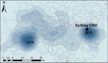
An alternative way to depict hot spots is by density maps. These are usually represented by raster layers, i.e. spatial grids subdivided in equally sized squares or rectangles (pixels or cells), in which each pixel (or cell) represents one value of a certain variable. The kernel density estimation (KDE) technique, often used in epidemiological studies, associates each point at which measurements of a relevant variable were taken, with a kernel function (Bailey and Gatrell, Reference Bailey and Gatrell1995; Chung et al. Reference Chung, Yang and Bell2004). This is expressed as a bivariate probability density function over an x−y plane, centred at each known point and decaying to a value of 0 over a defined bandwith (Fig. 3). Commercial off-the-shelf GIS have KDE functionality, but end-users must take informed decisions to select the kernel function and the bandwidth (also sometimes termed window area of the kernel). The most commonly used form of the kernel function K() is the quartic kernel (available in ArcGIS, for example), but the most critical parameter to select is the bandwidth, which influences the level of smoothing of the calculated surface (Allen and Wong, Reference Allen and Wong2006).

Fig. 3.

Example of kernel density estimation (KDE) raster calculated from raw (not standardized) data collected by Fletcher (Reference Fletcher2013), of cases of reported parasite illness in New South Wales (Australia) as recorded by four major hospitals located in the Sydney metropolitan area, serving the entire state. Cases were identified by post-codes. To perform KDE calculations the attributes of post-codes (polygons) were transferred to centroid points in the polygons. The kernel bandwidth value selected for the calculation in this example was 5·78×10⁻² dd. The two areas of highest density (darker shades of colour) represent highest probability of infection. The map was prepared using ArcGIS Desktop v. 9.3.

The spatial analysis tools described are used in geographic distribution studies of diseases or of the parasites causing infection and illness (e.g. Khan et al. Reference Khan, Davenhall, Ali, Castillo-Salgado, Vasquez-Prokopec, Kitron, Soares Magalhães and Clements2010), using an approach that is also common to ecology. This approach is justified also in view of the fact that many factors lead to human infections and often the diffusion of infection from parasite (or virus), to host animal, to human, spans several different environments (Guernier et al. Reference Guernier, Hochberg and Guégan2004; Wolfe et al. Reference Wolfe, Panosian Dunavan and Diamond2007), being also subject to host–parasite co-evolution (Poulin et al. Reference Poulin, Morand and Skorping2000; Nieberding and Olivieri, Reference Nieberding and Olivieri2007; Nieberding et al. Reference Nieberding, Durette-Desset, Vanderpoorten, Casanova, Ribas, Deffontaine, Feliu, Morand, Libois and Michaux2008; Morand, Reference Morand2012). Studies overlapping the fields of ecology (parasite habitat) and anthropology (human settlements and habits) rely on such analytical tools (e.g. Kitron et al. Reference Kitron, Otieno, Hungerford, Odulaja, Brigham, Okello, Joselyn, Mohamed-Ahmed and Cook1996; Dangendorf et al. Reference Dangendorf, Herbst, Reintjes and Kistemann2002; Demírel and Erdoğan, Reference Demírel and Erdoğan2009; Noor et al. Reference Noor, Mohamed, Mugyenyi, Osman, Guessod, Kabaria, Ahmed, Nyonda, Cook, Drakeley, Mackinnon and Snow2011; Wanjala et al. Reference Wanjala, Waitumbi, Zhou and Githeko2011; Gowland and Western, Reference Gowland and Western2012).

Exploration and analysis: semivariograms

Semivariograms are a particular category of diagrams used to reveal spatial autocorrelation: they can be used on their own, or as the preliminary exploratory step to the construction of interpolation surfaces (next sub-section). Taking the distance on the horizontal plane x−y between two generic points A and B to be:

$$\left| {\rm h} \right| = \sqrt {(x_A - \; x_B )^2 + (y_A - \; y_B )^2} $$

where (x _A , y_A ) and (x _B , y_B ) are the coordinates of A and B respectively, then the value of semivariance of a generic variable z measured at A and B is given by:

$$\gamma ({\rm h}) = \displaystyle{1 \over 2}[z_A - z_B ]^2. $$

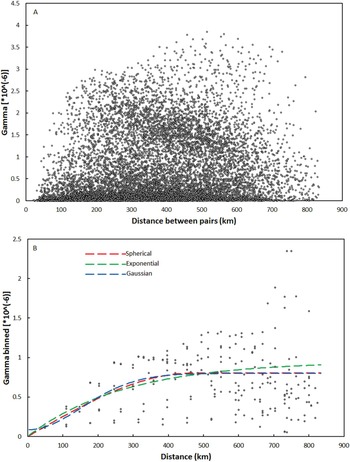
Plotting the values of semivariance for each pair of points against their distances, a semivariogram cloud is obtained (Fig. 4A), comprising {[n(n−1)]/2} data points, where n is the total number of measurements taken. No patterns are readily apparent from a semivariogram cloud, therefore binning is commonly carried out: this consists in grouping distances between point pairs into lags (distance intervals: h, 2 h, 3 h, etc.), and calculating the average value of semivariance for all the pairs included in each bin by:

$$\gamma ({\rm h}) = \displaystyle{1 \over {2n}}\sum\limits_{i = 1}^n {[z(I) - z(I + h)]} ^2 $$

where z(I)is the value of z at a generic location I, z(I+h) represents the value of z at all locations separated by lag distance h from I, and n is the number of pairs separated by distance h. The binned semivariances are then plotted against each lag and an empirical semivariogram is obtained (Fig. 4B). This diagram shows points distributed in a curved trajectory which can subsequently be fitted by a model function. The model function describes the way spatial autocorrelation decays away from each point up to a certain distance, known as range, marked by the plateauing (known as sill) of the model curve, beyond which geographic proximity no longer plays a role in the variable values.

Fig. 4.

Empirical and model semivariograms obtained for a set of 157 generic values z attributed to as many locations of geographic coordinates {x _i ; y_i }. The locations were randomly selected from a raster of real geographic measurements, shown in frame (B) of Fig. 7. (A) Semivariogram cloud. The diagram contains 12 067 data points. No patterns are readily apparent from the cloud, and no model curve can be established; (B) Binned semivariogram. The default values of lag for binning resulting from the Geospatial Analyst functionality of ArcGIS v. 9.3 have been adopted, but these can be varied. The binned semivariogram comprises 211 data points. Three smoothing model curves are drawn through the data points: spherical (red); exponential (green); Gaussian (blue). Both the spherical and exponential model curves start at the origin of the axes. The Gaussian model curve intersects the vertical axis at a value of 0·086×10⁶, which represents the nugget, i.e. the spatially uncorrelated variation or noise in the data (Pfeiffer et al. Reference Pfeiffer, Robinson, Stevenson, Stevens, Rogers and Clements2008). The distance at which each model curve flattens (the range) indicates the maximum lags at which pairs of points are expected to be spatially correlated: points separated by larger distances are not spatially correlated. In this example no model perfectly describes the variability of the values (which is generally the norm). Additional manipulation of the data is required, for example by changing parameters manually (in the GIS software) to obtain the best statistical fit (the one that minimizes the errors) between models and data.

A critical difficulty consists in choosing the extent of the set n(h): for the example shown in Fig. 4 the default values of lag for binning resulting from the Geospatial Analyst functionality of ArcGIS v. 9.3 have been adopted, but these can be varied. Manipulation of the data may be required, for example by changing parameters manually (in the GIS software) to obtain the best statistical fit (the one that minimizes the errors) between models and data. To use the algorithms correctly, a minimum of theoretical understanding of variography is required, but with little practice the semivariograms can be readily interpreted to extract significant information: for example, Oliver et al. (Reference Oliver, Muir, Webster, Parkes, Cameron, Stevens and Mann1992) computed the semivariogram of the incidence rates of childhood cancer in Britain to establish the spatial structure of the illness. They determined that the cases were not distributed randomly, but rather there was spatial dependence up to a distance of 50 km, as revealed by the fit of a model semivariogram to the empirical data. They concluded that spatial dependence was due to patches where risk was large (principally in rural areas) as opposed to zones of low risk, and that additional work was necessary to explain the patterns observed.

Analysis: interpolation

Spatial interpolation is the process by which known values at measured points (e.g. locations) are used to estimate values at other points where records are not available.

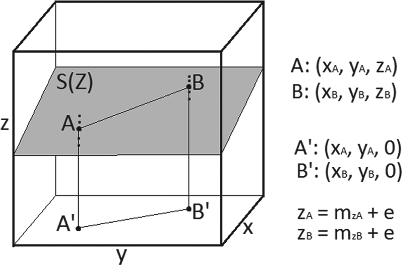
In a Cartesian space x–y–z, where the x–y plane is a generic horizontal plane, and z the axis perpendicular to it, a surface S(Z) represents all the values of the continuous variable z over all possible pairs of coordinates x–y, so that two generic points A and B of S(Z) have coordinates: (x _A , y_A, z_A ) and (x _B , y_B, z_B ), respectively (Fig. 5). Repeated measurements of the variable z at points A and B yield mean values m _zA and m _zB , so that the true values z _A and z _B are related to the means by:

(2) $$z_A = m_{zA} + e$$

(3) $$z_B = m_{zA} + e$$

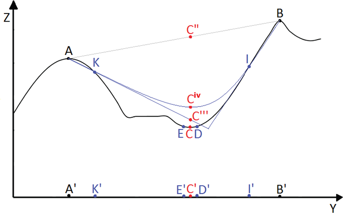
where e is the error on the measurements. If this error is only due to random fluctuations in the measurements, i.e. it is not caused by systematic problems owing to the operator or poor quality of instrumentation, then it is expected to be normally distributed, to have a mean value of 0, and variance σ ² [in mathematical notations: e∼N(0, σ ²)]. For a regular surface S(Z), for example like the surface shown in the figure, or a surface with a known analytical solution, it is sufficient to measure the values of z for a few points belonging to the surface, and then use a mathematical function to define the entire surface. If the surface shape is unknown or irregular then the values of z at points not measured must be calculated by interpolation: for example, the z-values for the points of S(Z) located between A and B (straight line connecting the two points in Fig. 5) can be calculated by linear interpolation. The number of interpolations to be carried out depends on the number of points measured, and increases with increasing number of measured points. Too few known points yield incorrect surfaces (Fig. 6); too many points require a very high number of computation steps, which may not always be technically possible.

Fig. 5.

Space x–y−z. A generic surface S(Z) is shown in grey. Two points (bold) A and B belong to the surface. Their projections on the horizontal x−y plane are A′ and B′, of coordinates: (x _A , y_A , 0) and (x _B , y_B , 0), respectively. The dots above and below points A and B indicate the values of z actually measured, so that mean values m _zA and m _zB of the variable z at both locations are calculated as the simple average of the measurements.

Fig. 6.

Cross-section of a generic irregular surface S(Z) on the y–z plane. The cross-section has peaks and troughs, and the positions of generic points belonging to the surface are indicated by capital letters. The same letters are used to indicate the projections of the points on the y axis. Linear interpolation between A and B is shown by a grey line connecting the two points. Blue lines represent interpolations using additional known points K and I. Unknown point C is shown in red.

The number of known points available, and type of interpolation function applied, influence the accuracy of the prediction about the true shape of the surface. If A and B are the only known points on irregular surface S(Z), then a linear interpolation between the two points produces a straight surface (grey line in Fig. 6), and the estimate of the values of z for all intermediate points will correspond to this interpolated surface. For a generic unknown point whose projection on the y-axis is C′, the interpolated value will be C″, very different from the true value represented by point C (red point in Fig. 6). The prediction is improved by adding measurements of z at points K and I. Two types of interpolation can be carried out: (a) linear interpolation between A and K, and between B and I, with the interpolating lines extrapolated until they intersect. On the new interpolated surface (straight blue lines in Fig. 6) the value of C is estimated to be C′″; (b) polynomial interpolation, represented by the curved blue line. On this new interpolated surface the value of C is estimated to be C ^iv. Both C′″ and C ^iv are much closer to the true value of z for C than the interpolated value obtained considering only known points A and B. However, also in this case, calculated values are not equal to the true value. It is also important to note that the polynomial function smoothes the interpolated surface, but at the cost of precision.

Estimates are obviously improved by measuring additional intermediate points, thus increasing the number of interpolations that must be carried out. Importantly, if the x–y–z space is geographic, with x and y representing geographic coordinates, and z any parameter varying with location, then one way to reduce the number of calculations required is to use the concept of spatial autocorrelation, illustrated by points C, D and E in Fig. 6: the value of z in unknown point C is expected to be more similar to the values of z for points D and E, in close proximity to C, than to those measured at points A, B, K and I. An alternative and equivalent way to express the concept of spatial autocorrelation is that, given a mathematical model (e.g. interpolation between A and B, or interpolations using also points K and I in the given example), deviation of the values of the variable z from the mathematical surface will be equal to the sum of the random measurement error e (equations 2 and 3) plus the error caused by spatial autocorrelation, so that we can re-write [equation 1] as:

(4) $$S(Z) = ({\rm Model_1} ) + ({\rm Spatial}\,{\rm autocorrelation} + e)$$

where S(Z) is the outcome and the second term in brackets in the right-hand member of the equation is the total error. Because e∼N (0, σ ²), and the model term (Model₁) can be represented by mathematical functions of known analytical solutions, the only term in [equation 4] which must be defined is that for spatial autocorrelation.

In the classical geostatistical approach spatial autocorrelation is evaluated from the measured data and compared to known models, so that:

(5) $${\rm Spatial}\,{\rm autocorrelation} = ({\rm Model_2} ) + er$$

where er expresses the random error er∼N (0, σ ²) for this equation. If the semivariance is taken as a measure of spatial autocorrelation, then some of the most used models (Model₂) to be fitted to the data are: spherical, exponential and Gaussian (Fig. 4). The best model will be one that minimizes er. The error term er is also known as residual variation, and it is usually defined in spatial analysis by the root mean square error RMSE. Standard GIS packages with spatial autocorrelation and semivariogram functionality will calculate the RMSE leaving it then to the users to decide on the significance of the results.

When also the model term (Model₁) in [equation 4] is selected among a predetermined family of functions and parameters whose combinations produce the best fit by minimization of the observed errors, we have the geostatistical method known as kriging (next section). Kriging functionality is routinely included in some of the most sophisticated GIS software (e.g. ArcGIS), and its operations are relatively user-friendly. Users are however required to enter manually a choice of parameters, and therefore there is a need to understand the logical steps required, otherwise the results will be meaningless: preliminary exploration of the data to hypothesize about the spatial structure (using the tools introduced in earlier sections), and ideas about the scientific reasons for patterns and clusters, need to inform the user.

Analysis: kriging

Kriging is an interpolation technique routinely included among the geostatistics tools of GIS software packages. An explanation of the principles of kriging as applied to epidemiology, and the sequence of the procedural steps involved, are illustrated by (for example) Carrat and Valleron (Reference Carrat and Valleron1992) and Rogers and Sedda (Reference Rogers and Sedda2012). In synthesis, kriging assumes that the spatial variation of an attribute consists of three components: a structure (or drift) representing the trend (included in the Model₁ term in [equation 4]), a spatially correlated (local) component and a random error term, as shown in [equation 4]. The trend (i.e. the model in the equation) provides an understanding of the regional processes; the locally correlated error is what we require for predictive purposes, as it measures the tendency for neighbouring values to be similar in their deviation from the global mean, as one would expect for clusters and hot spots.

As seen in the previous section, the spatially autocorrelated component is examined by semivariograms and a model is fitted to the data (Fig. 4). Most common models used in disease mapping studies are spherical (e.g. Standley et al. Reference Standley, Adriko, Alinaitwe, Kazibwe, Kabatereine and Stothard2009), exponential, or Gaussian (e.g. Allen and Wong, Reference Allen and Wong2006), although many more models are available in some GIS packages (e.g. ArcGIS has 11; Chang, Reference Chang2010). The selected semivariogram is then used for spatial interpolation by ordinary or universal kriging. Fitting of the semivariogram is an essential step for kriging (Rogers and Sedda, Reference Rogers and Sedda2012), but it may be marred by problems with extreme values, and user inexperience in selecting lags for the empirical semivariogram, and the appropriate model.

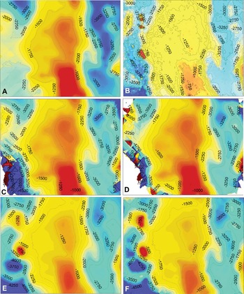
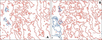
Ordinary kriging presupposes the absence of the drift component and uses the weighted average of values of a variable at neighbouring locations to evaluate unknown values in un-sampled locations. Universal kriging incorporates a first-order or second-order polynomial in the kriging process, to account for the drift component. Both kriging methods are used in studies of distribution of diseases (e.g. Kleinschmidt et al. Reference Kleinschmidt, Bagayoko, Clarke, Craig and Le Sueur2000; Zhong et al. Reference Zhong, Xue, Cao, Cao, Li, Guo, Fang, Sunderam, van Albada, Sloot and Dongarra2005; Allen and Wong, Reference Allen and Wong2006; Whitworth et al. Reference Whitworth, Symanski, Lai and Coker2011; Loiseau et al. Reference Loiseau, Harrigan, Bichet, Julliard, Garnier, Lendvai, Chastel and Sorci2013). These techniques have the advantage of being readily applied using the most common commercial or open source off-the-shelf GIS software. They also provide very useful insights regarding the locations and possible causes of foci of disease. However, application of these techniques requires some fundamental understanding of the concepts of spatial autocorrelation, how to deal with global and local trends, and what the resulting interpolation surfaces represent. Even when using a relatively friendly package such as ArcGIS, users are required to manually enter the parameters (or approve the default options) that the software will use to carry out interpolations. Different choices of parameters result in widely diverging results. Figures 7 and 8 illustrate an example of simple interpolation surfaces obtained from the same dataset: the calculated surfaces are all different from each other, and, more importantly, they are all different from the ‘real’ data-surface (frame B in Fig. 7). Consequently, the interpretation of the interpolation surfaces also needs to be supported by knowledge and understanding of the operations by which they were generated, and of the source and magnitude of the uncertainty inherent in the models. Because of the effect manual input of parameters has on the final outputs of kriging, the commercial GIS software provider ESRI has introduced a new functionality (EBK: empirical Bayesian kriging) in its ArcGIS Desktop version 10.1. The new tool uses simulations to estimate the semivariogram and the maps (Krivoruchko, Reference Krivoruchko2012), thus removing the need for users to input values and select models.

Fig. 7.

Comparison of results of different kriging models. The data used in (A), (C) and (D) are the same as in Fig. 4. A set of 160 location data was added (for a total of 317 locations) to construct the interpolation surfaces shown in (E) and (F). The interpolation surfaces are shown as false colour rasters, with higher values in red and lowest values in aqua-blue colours. The 3-dimensional shapes of the surfaces are also represented by contour lines, with contour intervals of 250 m. (A) Interpolation surface generated by ordinary kriging; (B) ‘Real’ surface. This is the original raster from which the data were extracted; (C) Interpolation surface generated by universal kriging with second-order global detrending; (D) Universal kriging obtained by second-order detrending with 50% global component and 50% local component; (E) Same as (A), but calculated using 317 locations; (F) Same as (C), but generated using 317 locations.

Fig. 8.

Difference surfaces. The differences between the ‘real’ surface and those generated by applying kriging modelling to a limited number of locations extracted from the raster, were calculated using Raster Calculator in ArcGIS v. 9.3. The differences are shown as contour lines. Red: no difference; blue: maximum differences. (A) Difference calculated using the ordinary kriging surface shown in (E) in Fig. 7; (B) Difference calculated using the ordinary kriging surface shown in (A). The largest differences occur in the western portion of the areas, but are less extensive and more limited in value for the interpolation surface modelled using a higher number of locations.

Analysis: co-kriging

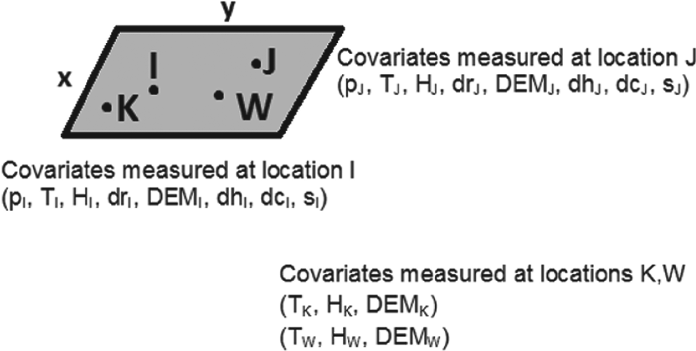
Let's assume that the following data are collected: prevalence of an illness (p); temperature (T); humidity (H); distance from a pond or river (dr); elevation (DEM); distance from hospital (dh); distance from major city (dc); any other environmental or social variable (s) at different locations I and J of coordinates: (x _I , y_I ) and (x _J , y_J ) (Fig. 9). All the parameters measured vary depending on location, so that an equation of the form of [equation 4] can be written for each of the variables. Also, there may or may not be a causal relationship between two or more of the variables. We are interested in mapping the prevalence of disease, and to generate an interpolation map whereby the prevalence may be estimated also where data are not collected, for example, at generic points K and W, where only temperature, humidity and elevation data are taken, but no prevalence or social variable data (Fig. 9). This is a common situation, because it often happens that disease or parasite data collection is sketchy. In these cases interpolation by classical geostatistical methods can be expected to produce unreliable maps, especially since sparse and extreme values majorly affect the semivariogram. Accessory environmental information layers instead are often data-rich (Rogers and Sedda, Reference Rogers and Sedda2012). The co-kriging technique, essentially a multivariate extension of kriging (Goovaerts, Reference Goovaerts2000), uses the spatial structure of the co-located variables to interpolate the primary variable of interest. For example, the spatial transmission of malaria in Iran was modelled with the help of information derived from elevation, temperature, vegetation and humidity layers (Barati et al. Reference Barati, Keshavarz-valian, Habibi-nokhandan, Raeisi, Faraji and Salahi-moghaddam2012). Co-kriging has also been applied to studies of rare diseases: Oliver et al. (Reference Oliver, Webster, Lajaunie, Muir, Parkes, Cameron, Stevens and Mann1998) used the incidence of childhood cancer data in Britain (an update of the data previously published by Oliver et al. Reference Oliver, Muir, Webster, Parkes, Cameron, Stevens and Mann1992) and evaluated the spatial variability of the unknown risk of cancer from the known proportions of cancer cases (number of cases/number of children in wards). Ortiz Valencia et al. (Reference Ortiz Valencia, De Paula Menezes Drumond Fortes and de Andrade Medronho2005) used co-kriging to incorporate secondary information (housewife's schooling years, household income, presence and use of home water filters, household density) to evaluate the spatial estimation of the risk of Ascariasis in Brazil. They found that co-kriging worked better than other techniques at identifying very high risk areas. Furthermore, they could correlate the additional information to the risk, establishing that lower socio-economic standards led to higher risk of the disease.

Fig. 9.

Sketch illustrating different information layer richness. The grey x−y space represents a continuous set of generic geographic coordinates. The points I, J, K and W represent locations where a set of co-located variables were measured. At locations I and J data for a full spectrum of environmental and social variables (see text) are collected, in addition to the parameter of interest, prevalence (p). At points K and W only data from a sub-set of environmental parameters (T: temperature, H: humidity, and DEM: elevation) are collected. The information layers for these parameters are richer than the layer for the parameter of interest and can be included in co-kriging (see text).

Explanation – model-based geostatistics

In the examples of interpolation and analysis described thus far the approach was empirical, with application of the techniques to the data, without assuming anything about the stochastic model generating the data. A different approach, termed model-based geostatistics (Diggle et al. Reference Diggle, Tawn and Moyeed1998), is based on the application of statistical inference principles to explicitly declared models of the data generating mechanisms. This approach to geostatistics requires deep knowledge of both the scientific discipline to which the model is to be applied, and of statistics, and it does involve close collaborations between statisticians and discipline practitioners (Diggle and Ribeiro, Reference Diggle and Ribeiro2007).

Both classical and Bayesian inference are applied in model-based geostatistics. In classical statistics the model is considered ‘real’ and the data collected are intended as one of the many possible realizations of the model. What is investigated is the probability of measuring the data, given a certain model:

$$P({\rm data}|{\rm Model})$$

The Bayesian approach to geostatistics can be thought of as the opposite:

$$P({\rm Model}|{\rm data})$$

whereby what is investigated is the probability that a certain model is true, given the data. The data are therefore ‘real’. Bayesian statistics relies on the concept of conditional probability, meaning that we use any prior information (i.e. existing or supposed and available) to help constrain the model (Glickman and van Dyk, Reference Glickman, van Dyk and Ambrosius2007). The relationship between the classical and Bayesian approach can be expressed as:

$$P({\rm Model}|{\rm data})\propto P({\rm data}|{\rm Model}) \times P({\rm Model})$$

where P(Model) represents the prior knowledge, and the term P(Model|data) is referred to as the posterior probability. The term: P(data|Model) is referred to as the likelihood. In iterative procedures the posterior is sampled and used as the prior in subsequent steps.

As a field of study, epidemiology makes extensive use of the Bayesian inference frame to model the importance of covariates and their effects on the spreading or risk of diseases. In the context of disease mapping, further complications arise because of spatial autocorrelation. Applications of the Bayesian inference frame to geostatistics are of varied type and extent, and it is outside the scope of this review to provide a complete summary. There are many complex aspects to the various ‘flavours’ of Bayesian analysis applied in the spatial analysis of disease, and it is necessary to gain a proper appreciation and understanding of all these aspects before using Bayesian techniques. Furthermore, Bayesian modelling is not conducted in the off-the-shelf user-friendly GIS software environment. However, Bayesian methods are now the common standard for modelling the spatial extent and risk of disease, and their existence must be acknowledged here for a complete picture. In addition, while it is certainly true that to fully implement Bayesian methods computing-intensive programming resources are needed, there are open-source packages available which, once set up for the specific problems to be addressed, can be used routinely in moderately powerful computer environments. Software such as WinBUGS (Lunn et al. Reference Lunn, Thomas, Best and Spiegenhalter2000), a specific package from the Bayesian inference Using Gibbs Sampling (BUGS) project, includes geospatial functionality (GeoBUGS; Thomas et al. Reference Thomas, Best, Lunn, Arnold and Spiegelhalter2004) into which data from other GIS software can be imported. Another readily useable open source software package is CARBayes (Lee, Reference Lee2013), available from the Comprehensive R Archive Network (CRAN) repository. Readers should consult the books by, for example, Diggle and Ribeiro (Reference Diggle and Ribeiro2007), Pfeiffer et al. (Reference Pfeiffer, Robinson, Stevenson, Stevens, Rogers and Clements2008) and Lawson (Reference Lawson2009), for a rigorous and exhaustive explanation of Bayesian methods in disease mapping and for WinBUGS examples and scripts.

Depending on the problem and the application, the spatial autocorrelation error may be included in the prior or in the likelihood terms. A conditional auto-regressive model (CAR) accounting for random effects associated to spatial autocorrelation is increasingly integrated in Bayesian methods (Pullan et al. Reference Pullan, Sturrock, Soares Magalhães, Clements and Brooker2012). The CAR considers area-specific random effects by way of adjacency weight matrices, such that more information is included in the calculations from closer areas than from farther areas. An evaluation of the most common models in the CAR class is given by Lee (Reference Lee2011). Another approach to modelling spatial dependence is given by the generalized linear spatial model (GLSM; Diggle et al. Reference Diggle, Tawn and Moyeed1998), a computer-intensive iterative method requiring professional statistical expertise. Bayesian models of increasing complexity have been developed over the years to improve the reliability of risk estimates, but most of the applications to disease mapping revolve around the use of the Besag, York and Mollie model (BYM) (Besag et al. Reference Besag, York and Mollie1991), often incorporated into statistical packages (Best et al. Reference Best, Richardson and Thomson2005; Leyland and Davies, Reference Leyland and Davies2005).

The scientific literature of spatial parasitology is rich in examples of studies mapping incidence and risk of illness (e.g. helminth infection, spatial distribution of malaria, mapping and risk of rare non-contagious diseases) using the Bayesian approach (e.g. Raso et al. Reference Raso, Matthys, N'Goran, Tanner, Vounatsou and Utzinger2005; Clements et al. Reference Clements, Moyeed and Brooker2006a , Reference Clements, Brooker, Nyandindi, Fenwick and Blair2008a , Reference Clements, Garba, Sacko, Touré, Dembelé, Landouré, Bosque-Oliva, Gabrielli and Fenwick b , Reference Clements, Deville, Ndayishimiye, Brooker and Fenwick2010; Brooker and Clements, Reference Brooker and Clements2009; Randremanana et al. Reference Randremanana, Richard, Rakotomanana, Sabatier and Bicout2010; Reid et al. Reference Reid, Haque, Clements, Tatem, Vallely, Masud Ahmed, Islam and Haque2010; Cramb et al. Reference Cramb, Mengersen and Baade2011; Soares Magalhães et al. Reference Soares Magalhães, Biritwum, Gyapong, Brooker, Zhang, Blair, Fenwick and Clements2011a , Reference Soares Magalhães, Clements, Patil, Gething and Brooker b , Reference Soares Magalhães, Langa, Sousa-Figueiredo, Clements and Vaz Nery2012; Stensgaard et al. Reference Stensgaard, Vounatsou, Onapa, Simonsen, Pedersen, Rahbek and Kristensen2011; Brooker et al. Reference Brooker, Pullan, Gitonga, Ashton, Koaczinski, Katabereine and Snow2012; Flegg et al. Reference Flegg, Patil, Venkatesan, Roper, Naidoo, Hay, Sibley and Guerin2013; Sturrock et al. Reference Sturrock, Pullan, Kihara, Mwandawiro and Brooker2013). It is impossible in this review to refer to all the available literature, but we encourage readers to explore the extensive body of publications in spatial disease mapping to gain further understanding of the principles underpinning interpretations and of the conditions and assumptions for application of the methods.

Model-based kriging has also been developed and used especially in the context of rare non-contagious diseases. Goovaerts (Reference Goovaerts2005, Reference Goovaerts2010, Reference Goovaerts2012) used a geostatistical approach, in which binomial or Poisson kriging models were calculated to map cancer incidence and cancer risk in the USA. In this approach semivariogram estimators and kriging algorithms are derived using binomial or Poisson models, depending on the nature of the data. Indicator kriging is applicable when data can be treated as categories (such as, presence or absence of late stage cancer, for example; Goovaerts, Reference Goovaerts2009b ). These models filter out the noise produced by small or unevenly distributed samples before smoothing the results of the analysis.

Goovaerts (Reference Goovaerts2005) and Goovaerts and Gebreab (Reference Goovaerts and Gebreab2008) have compared model-based kriging techniques to Bayesian methods. Generally, kriging methods perform better when the dataset is large. Also, data from different types of support structure, e.g. point data and aggregated data, are better treated by model-kriging (Goovaerts, Reference Goovaerts2010). Bayesian methods are preferred when data are sparse and highly clustered (e.g. Patil et al. Reference Patil, Gething, Piel and Hay2011).

SPATIO-TEMPORAL ANALYSIS

Predictions of risk of infection based on spatial analysis allow forecasting of where outbreaks will occur if there is no intervention (e.g. vaccination programmes, improvement of sanitation condition, etc.), thus providing health authorities with indications about where to deploy cure and containment measures. However, in the global environment of modern societies, local or regional containment of infectious diseases is not likely to have durable effects. Changes in population density, environmental conditions and connectivity, that can occur over time, influence the spread and transmission of disease beyond what would normally be considered natural barriers, such as geographic boundaries (continents separated by oceans), environmental boundaries (e.g. species areal extent limited to elevation ranges, deserts, or water courses, etc.) or social boundaries. Therefore, the spread of diseases (epidemics) needs to be studied by spatio-temporal simulations. These are outside the scope of this paper, but are worth mentioning briefly in regards to those aspects that require the collection and analysis of spatially distributed data.

If containment is possible, illness remains confined to clusters of incidence, and the spread of a disease follows a decay law, regulating the contagion as transmitted from infected individuals to other individuals in geographic proximity. The temporal evolution of the disease is based on distance transmission models, fundamentally equivalent to those related to spatial autocorrelation. Eventually the spread ends at physical boundaries or when sickness is eradicated (either by infected individuals being cured or extinct prior to transmission of the disease to other individuals). Any changes in the physical boundaries or re-emergence of infection cause renewed and further diffusion of the disease. This type of analysis is carried out in a hierarchical Bayesian framework incorporating spatially varying diffusion parameters (e.g. Hooten and Wikle, Reference Hooten and Wikle2008; Long et al. Reference Long, Robertson, Nathoo and Nelson2012).

Network models of disease spreading (Riley, Reference Riley2007) are applied when barriers break down or are crossed, and infections are transferred along networks (translocation). Diffusion and translocation have different effects: in a study of foot-and-mouth disease in Britain during the epidemic of 2001, Green et al. (Reference Green, Kiss and Kao2006) showed that local spread resulted in increase of density of the epidemic, with a small impact on its spatial extent. Vice versa, animal movement (e.g. by trading) in specific seasons was the principal factor responsible for expansion of the disease to nation-wide proportions. Applying agent-based models (Hooten and Wikle, Reference Hooten and Wikle2010a ) to simulate the spatio-temporal behaviour of epidemics in a hierarchical Bayesian framework, Hooten and Wikle (Reference Hooten and Wikle2010b ) determined that in the USA intrastate transmissions of influenza were linked to population density and average summer temperatures, while interstate transmission was higher in winter.

EFFECT OF CLIMATE CHANGE ON INFECTION DISTRIBUTION

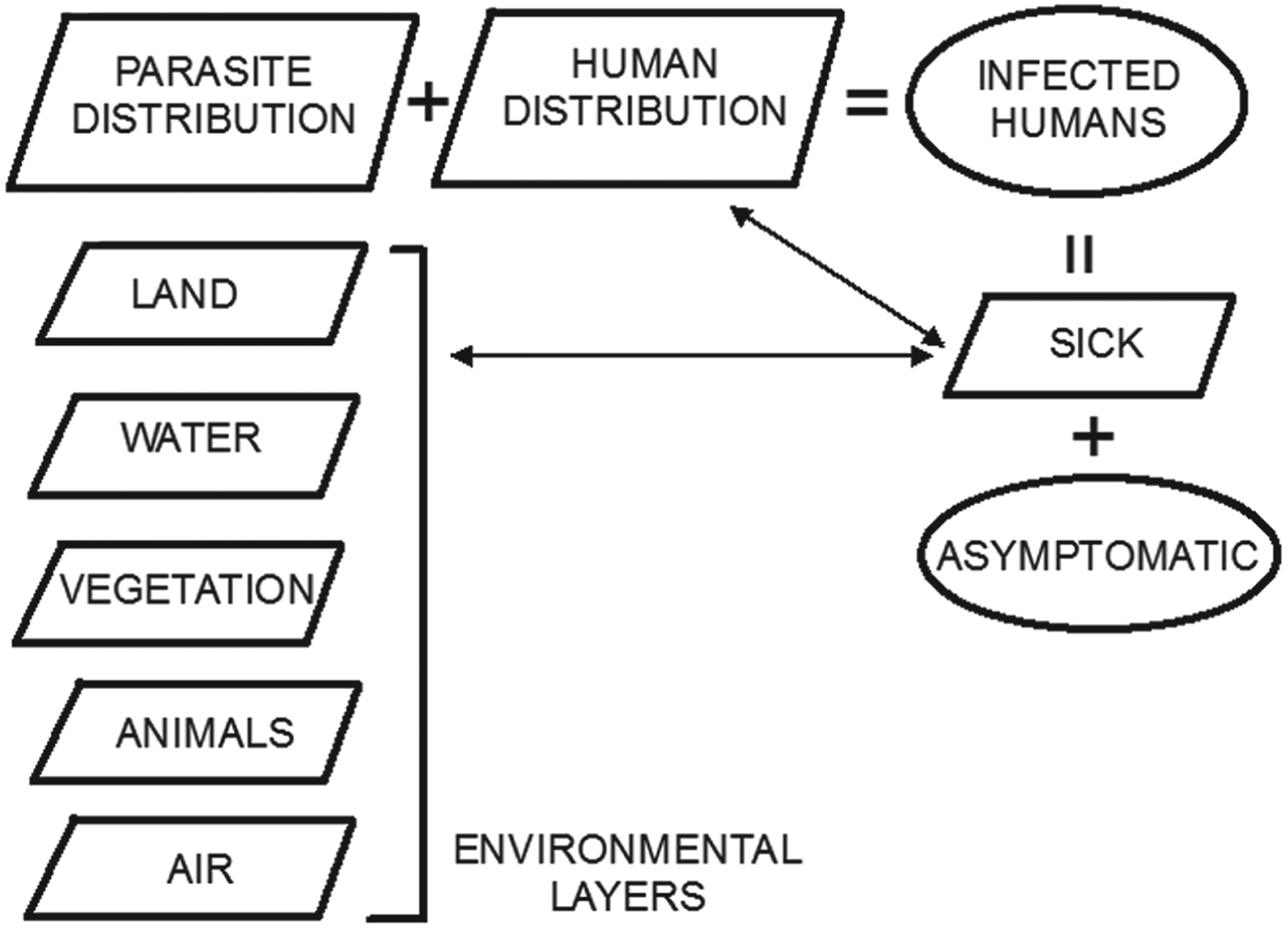
The spatial distribution of parasites (or viruses) is linked to local or global environmental conditions, and so are therefore the incidence and distribution of diseases in humans (Fig. 10). Environmental layers of information are normally acquired by remote sensing, using aerial surveys (limited in time and space) or Earth-observing satellites, which provide extensive coverage of all areas of Earth at periodic intervals, thus showing also changes in environmental conditions. Remote sensing datasets are normally available as rasters, which can be analysed together with other datasets using GIS software. The combination of remote sensing data acquisition and GIS is very powerful for rapid assessment of endemic areas, including those for which records of illness are difficult or impossible to obtain (Brooker et al. Reference Brooker, Hay and Bundy2002; Leonardo et al. Reference Leonardo, Rivera, Crisostomo, Sarol, Bantayan, Tiu and Bergquist2005; Yang et al. Reference Yang, Vounatsou, Zhou, Utzinger and Tanner2005).

Fig. 10.

Schematic diagram depicting the conceptual relationships between layers of information (parallelograms) for mapping in GIS, and sets (ovals) of infected humans. The ‘asymptomatic’ set represents hosts without illness, who may not be reported to health practitioners. Together with ‘sick’ individuals or groups, who are likely to be reported (and therefore who will be part of an information layer), these form the ‘infected humans’ set. The spatial distribution of the ‘sick’ humans is a sub-set of that of all the humans occupying the same space as parasites (or general infectious agents). The distribution of parasites is determined by the environmental conditions represented by various ‘environmental layers’.

With changing environmental conditions, diseases spread to previously uninfected locations, and new infections emerge (Jones et al. Reference Jones, Patel, Levy, Storeygard, Balk, Gittleman and Daszak2008; Long et al. Reference Long, Robertson, Nathoo and Nelson2012). The distribution of infection agents is tightly linked to climate conditions (e.g. Hu et al. Reference Hu, Clements, Williams, Tong and Mengersen2010; Métras et al. Reference Métras, Porphyre, Pfeiffer, Kemp, Thompson, Collins and White2012; Duncombe et al. Reference Duncombe, Clements, Davis, Hu, Weinstein and Ritchie2013). Consequently, changes in climate, causing migrations of animals, plants, and the parasites and viruses to which they are hosts, have a major effect on the spread of diseases. This has been well documented in ecological studies (e.g. Cudmore et al. Reference Cudmore, Björklund, Carroll and Lindgren2010: using spatially explicit simulation tools accounting for environmental conditions to model the infection of British Columbia conifers by beetles pests) and parasitology (e.g. Yang et al. Reference Yang, Vounatsou, Zhou, Utzinger and Tanner2005: using remote sensing environmental data collected over three decades to model the northward migration of the snail Oncomelania hupensis leading to an expansion of 40 000 km² of the area of potential transmission of Schistosoma japonicum in China). Other causes of environment modification, for example establishment of human settlements in pristine areas, deforestation, pollution of water courses, etc., also lead to habitat changes for parasites and their intermediate and final hosts, which can cause serious diseases in humans (e.g. Yang et al. Reference Yang, Clements, Gray, Atkinson, Williams, Barnes and McManus2012: anthropogenic activities leading to ecological changes in the hosts of Echinococcus spp. in China and consequent spread of disease to humans coming in contact with infected animals or their refuse). The ecological influences on the transmission and spread of disease owing to changes of climate or habitat disruption have been exemplified by Atkinson et al. (Reference Atkinson, Gray, Clements, Barnes, McManus and Yang2013) for the case of the global transmission of Echinococcus granulosus and Echinococcus multilocularis. Importantly, some diseases with long periods of latency and incubation can only be detected by mass screening of population before the illness manifests itself. This process is expensive, and not usually applied to areas with no history of infectious diseases, therefore rendering vain efforts at prevention. The only effective way to capture possible new foci of infection relies on predictive spatially explicit models taking into account temporal changes in environmental parameters affecting the distribution of parasites and hosts.

Planetary scale remote sensing datasets, increasingly made available free of charge and in formats readily exportable to mapping software, provide environmental layers of information that can be queried and modelled to identify patterns and high-risk locations. For example, cholera transmission is driven by complex interactions between abiotic, biotic and hydro-climatological factors, including the presence of biological and organic matter contributing to the growth of the bacteria in coastal waters. The quantity of biological and organic matter depends on location (latitude, presence of waterways causing floods, etc.), and follows patterns of seasonality that can be explored by remote sensing datasets, as Jutla et al. (Reference Jutla, Akanda, Huq, Faruque, Colwell and Islam2013) have done by introducing the Satellite Water Marker (SWM) index, calculated as the difference between satellite-measured radiance of clear and turbid water from Sea-viewing Wide Field-of-view Sensor (SeaWiFS) monthly radiance data. These authors have validated this index as an indicator in the prediction of cholera outbreaks for cases in Bangladesh and Mozambique. Other environmental indices (e.g. the Normalized Difference Vegetation Index, NDVI) calculated from remote sensing data are routinely used as proxies for environmental health or changes in environmental conditions, affecting the distribution of disease (e.g. Yang et al. Reference Yang, Vounatsou, Zhou, Utzinger and Tanner2005; Ekpo et al. Reference Ekpo, Mafiana, Adeofun, Solarin and Idowu2008). Data from a variety of satellite programs and sensors (e.g. Landsat series; MODerate Resolution Imaging Spectroradiometer, MODIS; Shuttle Radar Topography Mission, SRTM) can be used with imaging and mapping software to classify the use of land or to show changes in environmental parameters (e.g. temperature, elevation, aspect) with the purpose of evaluating environmental influences in the occurrence of hot spots of illness.

SPATIAL DECISION SUPPORT SYSTEMS

GIS has emerged as the preferred technology to build public health information geodatabases, and as the repository of analytical tools needed for real-time surveillance of infectious diseases (Khan et al. Reference Khan, Davenhall, Ali, Castillo-Salgado, Vasquez-Prokopec, Kitron, Soares Magalhães and Clements2010). Surveillance systems provide detection and control planning of infection outbreaks by integration of human and animal health data, visualization (mapping) and linkage between RGDB. The systems must be designed based on their objectives, which can be categorized in three principal areas: syndromic surveillance, eradication, endemicity (Robertson et al. Reference Robertson, Nelson, MacNab and Lawson2010). Syndromic surveillance relates to the monitoring of the frequency of a specified set of symptoms reported or discovered in a population unit without regard for the specific diagnosis (Reingold, Reference Reingold2003). The symptoms may be reported by practitioners, extracted from hospital records, from emergency calls (e.g. to ambulance or police), from neighbours, colleagues or school reports, and from purchases of over-the-counter medications. The purpose of syndromic surveillance is to evaluate the patterns that may lead to cases of outbreaks, and the focus of the data collection is the detection of time/space clustering of infection, defined as a higher than expected number or rate of events relative to a given (pre-determined) background value. The purpose of eradication is related to efforts to detect agents of infection and eventually eradicate them and prevent their return by removing the causes and conditions of their survival. In this case the response triggered by each individual case detected (e.g. reporting by a public health officer of a symptomatic patient) is recorded in the surveillance system. In areas of endemicity the monitoring is based on space-time trends, for example linked to seasonality. The tools to perform analyses and predictions require variable levels of sophistication in regards to the purpose of the surveillance system and to the type of illness to be monitored.

In 1993 the WHO launched a public health mapping programme, following up with further regulations for governments to implement use of early warning systems and efficient information technology for detection and surveillance of infectious diseases (Reinhardt et al. Reference Reinhardt, Elias, Albert, Frosch, Harmsen and Vogel2008). About 58% of world nations have since adopted GIS software in their disease surveillance (Khan et al. Reference Khan, Davenhall, Ali, Castillo-Salgado, Vasquez-Prokopec, Kitron, Soares Magalhães and Clements2010). Syndromic surveillance systems have a high level of noise, due to the fact that the data reported are not necessarily linked to a specific diagnosis of illness. The data used in these systems require therefore specific statistical and computational capacity. A free software package commonly used in syndromic surveillance (e.g. Horst and Coco, Reference Horst and Coco2010) is SaTScan (Kulldorff, Reference Kulldorff, Glaz and Balakrishnan1999), based on spatial scan statistics of points (e.g. reported symptoms) tested against a Bernoulli or Poisson model for randomness (Kulldorff, Reference Kulldorff1997), which can be also extended through time. In essence, if the distribution of reports is statistically distinct from a random distribution, clustering is inferred. To evaluate the statistical significance of detected clusters (P-values) SaTScan uses Monte Carlo iterations. This spatial scan software can be directly incorporated in the architecture of surveillance systems: the online GIS tool EpiScanGIS has been launched in Germany in 2006 as an early warning system for the monitoring and control of meningococcal disease (Reinhardt et al. Reference Reinhardt, Elias, Albert, Frosch, Harmsen and Vogel2008), and its central data-cluster analysis functionality is provided by SaTScan. The WHONET-SaTScan laboratory information software is made available by the WHO and has been used for detection of outbreaks from hospital-acquired infections (Huang et al. Reference Huang, Yokoe, Stelling, Placzek, Kulldorff, Kleinman, O'Brien, Calderwood, Vostok, Dunn and Platt2010).

The goal of eradication is to halt transmission, so surveillance systems must detect, classify and attack individual cases and foci of infection. In 1995 the WHO Office for the Americas launched an initiative to encourage the use of GIS for analysis of epidemiological data, leading to the development of a public-domain software package named SIGEpi (Geographic Information System in Epidemiology), offering simplified mapping and analysis tools (Martinez et al. Reference Martinez, Vidaurre, Najera, Loyola, Castillo-Salgado and Eisner2001). This tool is being used for the surveillance and control of malaria in Brazil, where the programme includes standardization of georeferenced information on mosquito breeding sites and house proximities, as well as training of local staff in the use of SIGEpi (Khan et al. Reference Khan, Davenhall, Ali, Castillo-Salgado, Vasquez-Prokopec, Kitron, Soares Magalhães and Clements2010). Customized GIS-based spatial decision support systems (SDSS) have also been developed to target malaria in Vanuatu (Kelly et al. Reference Kelly, Hale, Donald, Batarii, Bugoro, Nausien, Smale, Palmer, Bobogare, Taleo, Vallely, Tanner, Vestergaard and Clements2013), where confirmed malaria cases were reported to dedicated offices and routinely updated into the geodatabase.

Two global-scale important international projects involving world datasets are the Malaria Atlas Project (MAP; http://www.map.ox.ac.uk/about-map/) and the Global Atlas of Helminth Infections (GAHI; http://www.thiswormyworld.org/). The first project (Hay and Snow, Reference Hay and Snow2006), managed at the University of Oxford, UK, brings together researchers interested in developing techniques to map and understand the distribution and spread of malaria, with the aim to support effective planning of malaria control. The web-portal includes maps and the on-line tools to update new data to each map to ensure surveillance and control decisions are based on the most current information. There is also an updated list of publications by scientists contributing to the project. A data modelling section is available for advanced users to download programs and instructions to apply the spatial analysis concepts on new datasets. The GAHI is managed at the London School of Hygiene and Tropical Medicine, in the UK. It provides access to survey data maps, predictive risk maps and control and planning maps. These maps can be updated by contributing new data via emails addressed to the project team. A list of publications is also kept up to date. Important initiatives such as training in mapping and the use of epidemiological tools are also organized by the project team.

There are obviously very strong reasons for global mapping of diseases for monitoring and control purposes. However, in spite of some advanced projects (e.g. MAP and GAHI above) only about 4% of all diseases whose control would benefit from spatial analysis have been systematically mapped (Hay et al. Reference Hay, Battle, Pigott, Smith, Moyes, Bhatt, Brownstein, Collier, Myers, George and Gething2013). Naturally patchiness in the baseline picture of diseases cannot lead to effective global countermeasures, which is unfortunate and dangerous, given the global dimension of infectious diseases in a world in which spatial boundaries are becoming blurred. It is important that the example of disease mapping projects and research highlighted above is followed at national and international levels. We hope this review contributes to convince more health practitioners to embrace mapping and spatial analysis techniques, and more governments and world organizations to provide the resources for finer-scale health data collection.

DATA-DRIVEN AND KNOWLEDGE-DRIVEN MODELS

One useful way to look at how spatial analysis has been used, is to group disease spatial analysis studies into data-driven models and knowledge-driven models, as done, for example, by Métras et al. (Reference Métras, Collins, White, Alonso, Chevalier, Thuranira-McKeever and Pfeiffer2011) in their review of models of risk for Rift Valley Fever.

Data-driven spatial models use statistical methods to define the relationships between causes of illness and the distribution of illness (Pfeiffer et al. Reference Pfeiffer, Robinson, Stevenson, Stevens, Rogers and Clements2008). These models are based on actual incidence or prevalence data.

Knowledge-driven models are based on existing knowledge, or on the hypothesized understanding of the causal relationships leading to the emergence of disease (Pfeiffer et al. Reference Pfeiffer, Robinson, Stevenson, Stevens, Rogers and Clements2008). These models by definition do not require records of actual illness (or infection), except for the purpose of validation, and are therefore applied in cases where data are scarce or cannot be obtained. Knowledge-driven models basically indicate the suitability of an area for the emergence or spreading of disease, and are useful therefore to: (1) identify locations for future acquisition of intensity of infection or prevalence of infection data; (2) identify locations where containment efforts will produce the best results. Once the data are acquired and fed into knowledge-driven models, these are progressively refined into data-driven models. Knowledge-driven models rely heavily on environmental layers of information, generally acquired by remote sensing, which covers large areas, including those that cannot be easily reached on the ground. The environmental layers are generally examined to evaluate the sum of overlapping conditions favourable to the spreading of infection agents (parasites, intermediate host, etc.), and to the areal expansion of their habitats. In a few cases some of the techniques explored in the previous sections (e.g. decision analysis techniques), or fuzzy logic (e.g. Clements et al. Reference Clements, Pfeiffer and Martin2006b ), have also been included to complement knowledge-driven models, to determine the location of outbreaks.