1 Introduction
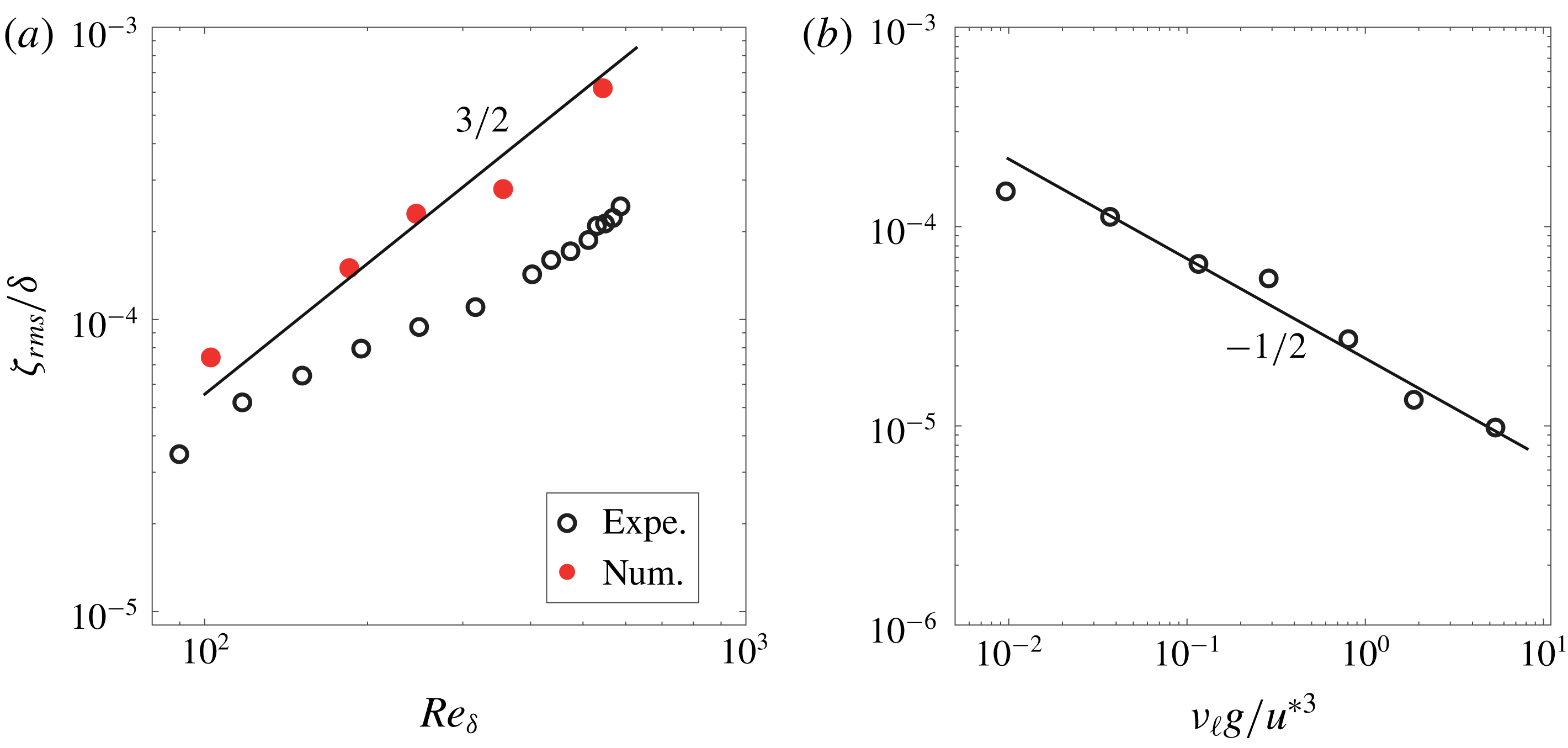
A mirror like liquid surface is quite rare to observe in outdoor conditions. The smallest breeze already perturbs the surface of water well below the onset of wave formation, as first described by Russell (Reference Russell1844). Since Russel’s work, this weak deformation regime below the wave onset has been often reported (Keulegan Reference Keulegan1951; Gottifredi & Jameson Reference Gottifredi and Jameson1970; Kahma & Donelan Reference Kahma and Donelan1988; Zhang Reference Zhang1995; Caulliez, Makin & Kudryavtsev Reference Caulliez, Makin and Kudryavtsev2008) but its precise spatio-temporal properties have been measured only recently by Paquier, Moisy & Rabaud (Reference Paquier, Moisy and Rabaud2015) who named these deformations wrinkles. Characterised by randomly distributed, elongated structures in the streamwise direction, the apparent disordered aspect of the wrinkles were interpreted qualitatively as a signature of the air turbulence on the liquid surface. An important feature of wrinkles is their dependence on the liquid viscosity
 $\unicode[STIX]{x1D708}_{\ell }$
. An empirical relation was inferred for the mean square amplitude (Paquier, Moisy & Rabaud Reference Paquier, Moisy and Rabaud2016),
 $$\begin{eqnarray}\displaystyle \overline{\unicode[STIX]{x1D701}^{2}}\propto \unicode[STIX]{x1D708}_{\ell }^{-1}u^{\ast 3}, & & \displaystyle\end{eqnarray}$$
where
 $u^{\ast }$
is the friction velocity of the air (Schlichting Reference Schlichting2000) and
 $\overline{\unicode[STIX]{x1D701}^{2}}$
is averaged over space and time. To the best of our knowledge, this empirical expression has not been explained theoretically.
Since wrinkles are systematically found even at moderate wind, they naturally represent a base state on which regular (quasi-monochromatic) waves propagating in the wind direction may grow. The influence of this initial perturbed surface state on the wave onset can be indirectly analysed by varying the liquid viscosity. Indeed, in the general understanding of the physical origin of the wind wave onset, the dependency in liquid viscosity is still lacking (Sullivan & McWilliams Reference Sullivan and McWilliams2010). While it has been observed experimentally that the liquid viscosity influences the wave onset (Francis Reference Francis1956; Kahma & Donelan Reference Kahma and Donelan1988; Veron & Melville Reference Veron and Melville2001; Paquier et al. Reference Paquier, Moisy and Rabaud2016), the explicit dependency has not been captured by models that include viscous effects (Lindsay Reference Lindsay1984; Funada & Joseph Reference Funada and Joseph2001; Kim, Padrino & Joseph Reference Kim, Padrino and Joseph2011).
In the literature of wind wave generation, two families of models can be identified. They involve either stability analysis of the mean wind profile or turbulent fluctuations. The branching goes back to the two seminal papers of Miles (Reference Miles1957) and Phillips (Reference Phillips1957) who proposed each a mechanism for wind wave generation. On the one hand, the stability analysis based on the mean wind profile in Miles models (Miles Reference Miles1993) or on the general Orr–Sommerfeld equation (see, e.g. Manneville Reference Manneville2010) ignores the turbulent fluctuations. Linear stability analysis predicts an onset above which the wave amplitude grows exponentially in time. A qualitative agreement with Miles theory has been obtained in laboratory experiments (Kawai Reference Kawai1979; Veron & Melville Reference Veron and Melville2001). However, a quantitative agreement of refined Miles models (Janssen Reference Janssen2004) with experimental data is still lacking both in laboratory conditions (Plant Reference Plant1982; Liberzon & Shemer Reference Liberzon and Shemer2011) and in outdoor conditions (Sullivan & McWilliams Reference Sullivan and McWilliams2010). On the other hand, Phillips, following Eckart (Reference Eckart1953), analysed the effect of random pressure fluctuations at the surface of an inviscid liquid. He considered a resonance mechanism between the surface displacement
 $\unicode[STIX]{x1D701}$
and the pressure fluctuations
 $p$
. He derived an expression for the mean square surface displacement of the form
 $$\begin{eqnarray}\displaystyle \overline{\unicode[STIX]{x1D701}^{2}}=\frac{1}{\unicode[STIX]{x1D70C}_{\ell }^{2}}\frac{\overline{p^{2}}t}{2\sqrt{2}U_{c}g}, & & \displaystyle\end{eqnarray}$$
where
 $\overline{p^{2}}$
is the mean square pressure fluctuation averaged over space,
 $\unicode[STIX]{x1D70C}_{\ell }$
the liquid density,
 $U_{c}$
the typical convection speed of the turbulent structures and
 $g$
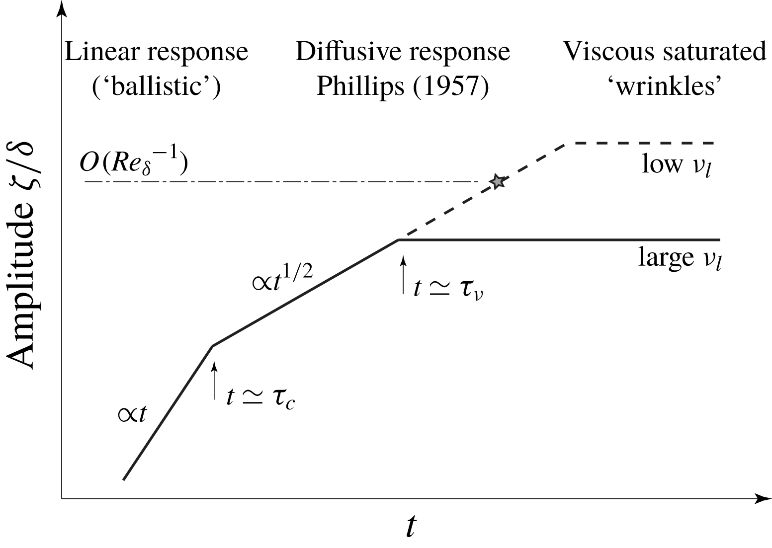
the acceleration due to gravity. Phillips theory yields a linear growth for the wave energy. Contrary to Miles theory, Phillips theory has not been extensively tested. Experimentally, algebraic temporal growth for the surface deformation has been observed recently by Zavadasky & Shemer (Reference Zavadasky and Shemer2017). Recent direct numerical simulations of two phase shear flows have also observed a regime of algebraic growth in time (Lin et al.
Reference Lin, Moeng, Tsai, Sullivan and Belcher2008; Zonta, Soldati & Onorato Reference Zonta, Soldati and Onorato2015) that may be attributed to Phillips mechanism. However, a quantitative agreement with Phillips theory has not been reported to date.
Phillips formalism may apply to the wrinkle regime, as the air flow is already turbulent for wind below the wave threshold, so that a resonance between pressure fluctuations and surface waves could already occur at low wind speed. Equation (1.2) provides a theoretical expression for
 $\unicode[STIX]{x1D701}$
that depends on time and is independent of viscosity, whereas (1.1) provides an empirical relation for
 $\unicode[STIX]{x1D701}$
that depends on viscosity and is independent of time. These two equations are therefore far apart elements of the wrinkle puzzle. The aim of this paper is to provide a theoretical framework for the wrinkle regime that reconciles (1.1) and (1.2).
A quantitative description of the wrinkle regime, even though it does not involve any instability mechanism, is challenging for mainly two reasons. First, the formalism must describe the response of a viscous liquid to an arbitrary forcing both in time and in space. For an impulsive forcing of arbitrary shape one can follow the approach of Miles (Reference Miles1968), who revisited the Cauchy–Poisson problem (Lamb Reference Lamb1995) for a viscous liquid. The response to a continuous perturbation in time can also be computed using the same formalism by linear superposition. However, the Fourier–Laplace transform formalism used by Miles limits the analytical feasibility to asymptotic solutions. For the specific case of a pressure source travelling at constant velocity, the wave pattern generated at the surface of an inviscid liquid was computed by Havelock (Reference Havelock1919). This classical problem, which provides a simplified description of the far-field wake behind a ship, has been recently revisited, for an inviscid (Raphaël & de Gennes Reference Raphaël and de Gennes1996; Rabaud & Moisy Reference Rabaud and Moisy2013; Darmon, Benzaquen & Raphaël Reference Darmon, Benzaquen and Raphaël2014) or a viscous (Richard & Raphaël Reference Richard and Raphaël1999) fluid. To the best of our knowledge, no such Havelock-like formulation is yet available for an arbitrary forcing pattern both in time and in space. Moreover, the Havelock formulation applies only for a pressure disturbance, whereas both pressure and shear stress act on the surface of a viscous liquid.
The second main difficulty arises from the modelling of the turbulence in the air boundary layer. Of particular interest for the wave generation problem is the slow dynamics and the long-range correlations of the pressure and shear stress fluctuations in the boundary layer. Their main statistical properties (characteristic size, mean convection velocity) have been measured since the 60s, e.g. by Willmarth & Wooldridge (Reference Willmarth and Wooldridge1962) and Corcos (Reference Corcos1963); see Robinson (Reference Robinson1991) for a comprehensive review prior to the development of numerical simulations. These early quantitative measurements, obtained from single-point probes, however, could not provide a full spatio-temporal characterisation of the turbulent fluctuations in a boundary layer.
In recent years, in-depth knowledge has been gained from direct numerical simulations (DNS), both for developing turbulent boundary layers and for fully developed turbulent channel flows (Choi & Moin Reference Choi and Moin1990; Moser, Kim & Mansour Reference Moser, Kim and Mansour1999; Jimenez, Del Alamo & Flores Reference Jimenez, Del Alamo and Flores2004; Jimenez & Hoyas Reference Jimenez and Hoyas2008). The maximum turbulent Reynolds number reached in the most advanced simulations,
 $Re_{\unicode[STIX]{x1D70F}}\simeq 4000{-}8000$
(Lozano-Durán & Jiménez Reference Lozano-Durán and Jiménez2014; Lee & Moser Reference Lee and Moser2015; Yamamoto & Tsuji Reference Yamamoto and Tsuji2018), is comfortably larger than the relevant values for the wind wave generation problem (
 $Re_{\unicode[STIX]{x1D70F}}\simeq 100{-}1000$
). Such data are highly valuable for the study of the wrinkle regime, as the air turbulence can be considered as essentially unaffected by the wave motion. Indeed, the typical surface displacement amplitude is much smaller than the viscous sublayer thickness in the air flow. This is precisely the regime explored in this paper. The situation is different for larger amplitude, close to the wave onset, for which a feedback of the wave motion on the air turbulence is expected, requiring a full two-phase flow approach. This approach, much more demanding computationally speaking, has been investigated recently (Belcher & Hunt Reference Belcher and Hunt1998; Kudryavtsev & Makin Reference Kudryavtsev and Makin2002; Lin et al.
Reference Lin, Moeng, Tsai, Sullivan and Belcher2008; Druzhinin, Troitskaya & Zilitinkevich Reference Druzhinin, Troitskaya and Zilitinkevich2012; Kudryavtsev, Chapron & Makin Reference Kudryavtsev, Chapron and Makin2014; Sajjadi et al.
Reference Sajjadi, Robertson, Harvey and Brown2017). Because of the high computational cost, the range of physical parameters covered by these studies remains limited, and no scaling relation has yet been obtained for the wave onset.
An important feature in the generation of surface waves by the wind is the unavoidable presence of a mean advecting current in the liquid, which may significantly affect the wave dynamics (Peregrine Reference Peregrine1976; Kirby & Chen Reference Kirby and Chen1989; Ellingsen & Li Reference Ellingsen and Li2017). The growth and saturation of a drift velocity in the liquid and wave growth are two closely intertwined processes (Banner & Peirson Reference Banner and Peirson1998; Melville, Shear & Veron Reference Melville, Shear and Veron1998; Veron & Melville Reference Veron and Melville2001), and the stability of the flow depends on the resulting velocity profiles both in the air and in the liquid (Miles Reference Miles1993). However, in the wrinkle regime explored by Paquier et al. (Reference Paquier, Moisy and Rabaud2015), the drift velocity is bounded to a few cm/s by the finite channel depth and the large viscosity of the fluid. Such drift velocity remains small compared to both air velocity and phase velocity of the wrinkles, and is neglected in the present study.
In this paper we focus on a quantitative description of the wrinkle regime, below the wind wave onset. For that purpose, we combine analytical calculations of the viscous response of the liquid to an arbitrary forcing in a statistically stationary state with DNS data of a turbulent channel flow. Based on careful dimensional analysis and experimental data of the wrinkle regime, we show that below the wave threshold the evolution of the turbulent air boundary layer can be decoupled from the liquid response. We thus circumvent the difficulty to simulate a full turbulent two-phase flow by considering a turbulent channel flow with rigid walls and no-slip boundary conditions. Doing so, we greatly simplify the numerical set-up to focus on the linear, passive response of the liquid phase. We show that the wrinkle statistics computed from our model are in good agreement with the experimental data of Paquier et al. (Reference Paquier, Moisy and Rabaud2015, Reference Paquier, Moisy and Rabaud2016). Finally, we show that the onset of regular waves may correspond to the breakdown of the regime of linear passive response of the liquid surface, and propose an empirical criterion based on surface roughness originating from the wrinkle amplitude.
The paper is organised as follows. Section 2 provides a general dimensional analysis of the surface deformation generated by a turbulent boundary layer. In § 3 we derive the key equation of the paper, that establishes the link between the Fourier components of the normal and tangential shear stresses applied at the air–liquid interface and the Fourier components of the surface displacement. Section 4 presents the direct numerical simulations used to compute the normal and tangential stresses. Section 5 combines the equation for the surface displacement in Fourier space and the output of the DNS to compute the wrinkle properties. It provides a quantitative comparison with the experiments of Paquier et al. (Reference Paquier, Moisy and Rabaud2016). Section 6 finally bridges the gap between the wrinkle regime governed by viscosity and the inviscid resonant theory of Phillips (Reference Phillips1957).
2 Wrinkle regime: dimensional analysis and experimental set-up
2.1 Dimensional analysis
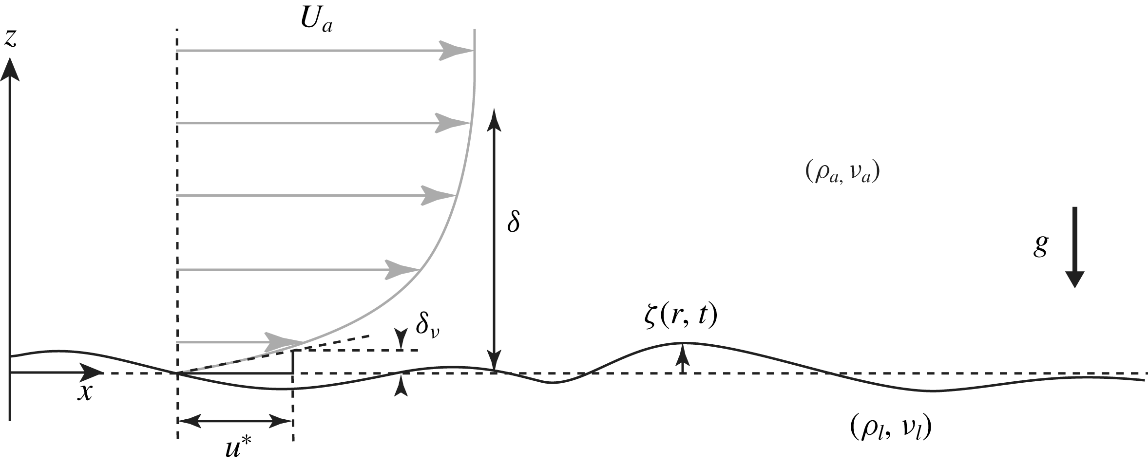
Sketch of the velocity profile of a turbulent wind blowing on a viscous liquid. The turbulent boundary layer is characterised by the outer layer thickness
 $\unicode[STIX]{x1D6FF}$
and the viscous sublayer thickness
 $\unicode[STIX]{x1D6FF}_{\unicode[STIX]{x1D708}}=\unicode[STIX]{x1D708}_{a}/u^{\ast }$
. The friction velocity
 $u^{\ast }$
is defined from the mean shear stress
 $\unicode[STIX]{x1D70F}_{a}=\unicode[STIX]{x1D70C}_{a}{u^{\ast }}^{2}$
at the wall. The liquid response may depend on the air/liquid densities
 $\unicode[STIX]{x1D70C}_{a},\unicode[STIX]{x1D70C}_{\ell }$
, the kinematic viscosities
 $\unicode[STIX]{x1D708}_{a},\unicode[STIX]{x1D708}_{\ell }$
, as well as
 $\unicode[STIX]{x1D6FF},u^{\ast }$
, the gravity
 $g$
and the surface tension
 $\unicode[STIX]{x1D6FE}$
.

We first discuss here the dependence of the surface displacement
 $\unicode[STIX]{x1D701}$
on the relevant physical parameters using dimensional analysis. In the statistically steady state, the characteristic amplitude of the surface displacement averaged over space and time
 $\unicode[STIX]{x1D701}_{rms}=(\overline{\unicode[STIX]{x1D701}^{2}})^{1/2}$
in response to a turbulent wind is expected to depend on numerous parameters that characterise both the turbulent flow in the air and the liquid properties. The geometry and the relevant parameters of both phases are sketched in figure 1. The turbulent air boundary layer is characterised by the air density
 $\unicode[STIX]{x1D70C}_{a}$
, the kinematic viscosity
 $\unicode[STIX]{x1D708}_{a}$
, the friction velocity
 $u^{\ast }=\sqrt{\unicode[STIX]{x1D70F}_{a}/\unicode[STIX]{x1D70C}_{a}}$
(where
 $\unicode[STIX]{x1D70F}_{a}$
is the mean shear stress at the interface) and the boundary-layer thickness
 $\unicode[STIX]{x1D6FF}$
. In a developing boundary layer, the thickness
 $\unicode[STIX]{x1D6FF}$
is function of the streamwise distance
 $x$
, usually called fetch in the wind wave generation problem, whereas it is constant in a fully developed channel flow. The spatial variation of a developing boundary layer is usually small (
 $\text{d}\unicode[STIX]{x1D6FF}/\text{d}x\ll 1$
), so we can simply consider the boundary-layer thickness
 $\unicode[STIX]{x1D6FF}$
as constant. The liquid flow is characterised by the liquid density
 $\unicode[STIX]{x1D70C}_{\ell }$
, kinematic viscosity
 $\unicode[STIX]{x1D708}_{\ell }$
, acceleration of gravity
 $g$
, surface tension
 $\unicode[STIX]{x1D6FE}$
and liquid depth
 $h$
.
Under these hypotheses, the amplitude of the surface displacement writes
 $\unicode[STIX]{x1D701}_{rms}=f(\unicode[STIX]{x1D70C}_{a},\unicode[STIX]{x1D70C}_{\ell },\unicode[STIX]{x1D708}_{a},\unicode[STIX]{x1D708}_{\ell },\unicode[STIX]{x1D6FF},u^{\ast },g,\unicode[STIX]{x1D6FE},h)$
. According to Buckingham’s
 $\unicode[STIX]{x03C0}$
theorem, the dimensionless surface displacement
 $\unicode[STIX]{x1D701}_{rms}/\unicode[STIX]{x1D6FF}$
can be expressed as a function of six independent dimensionless numbers. Choosing a set of dimensionless numbers that decouple the influence of the friction velocity
 $u^{\ast }$
and of the length scale
 $\unicode[STIX]{x1D6FF}$
, it writes
 $$\begin{eqnarray}\displaystyle \frac{\unicode[STIX]{x1D701}_{rms}}{\unicode[STIX]{x1D6FF}}=f_{1}\left(\frac{\unicode[STIX]{x1D70C}_{a}}{\unicode[STIX]{x1D70C}_{\ell }},\frac{g\unicode[STIX]{x1D6FF}^{3}}{\unicode[STIX]{x1D708}_{\ell }^{2}},\frac{{u^{\ast }}^{3}}{g\unicode[STIX]{x1D708}_{\ell }},Re_{\unicode[STIX]{x1D6FF}},Bo,\frac{h}{\unicode[STIX]{x1D6FF}}\right), & & \displaystyle\end{eqnarray}$$
where
 $f_{1}$
is a dimensionless function,
 $Re_{\unicode[STIX]{x1D6FF}}=u^{\ast }\unicode[STIX]{x1D6FF}/\unicode[STIX]{x1D708}_{a}$
is the turbulent Reynolds number characterising the boundary layer and
 $Bo=\unicode[STIX]{x1D6FF}/\ell _{c}$
is the Bond number (with
 $\ell _{c}=\sqrt{\unicode[STIX]{x1D6FE}/\unicode[STIX]{x1D70C}_{\ell }g}$
the capillary length). The relative depth
 $h/\unicode[STIX]{x1D6FF}$
becomes relevant for surface wave propagation in the shallow-water regime. We are mostly interested here in the the deep-water regime (one has
 $h/\unicode[STIX]{x1D6FF}\simeq 1.2$
in the experiment, see § 2.2), so the importance of this parameter is marginal in the following.
The function
 $f_{1}$
can be further specified using additional physical arguments. In the static case and without surface tension, the density ratio
 $\unicode[STIX]{x1D70C}_{a}/\unicode[STIX]{x1D70C}_{\ell }$
sets the surface displacement amplitude as can be seen from a simple pressure balance: the gravity pressure scales as
 $\unicode[STIX]{x1D70C}_{\ell }g\unicode[STIX]{x1D701}$
and the pressure fluctuations in the air phase scales as
 $\unicode[STIX]{x1D70C}_{a}{u^{\ast }}^{2}$
. Adding the surface tension introduces a dependency in Bond number but it does not modify the scaling of
 $\unicode[STIX]{x1D701}_{rms}$
in
 $\unicode[STIX]{x1D70C}_{a}/\unicode[STIX]{x1D70C}_{\ell }$
. In the dynamical case with negligible effect of gravity in the air phase, and in the limit of linear equation of motion, the displacement still scales as
 $\unicode[STIX]{x1D70C}_{a}/\unicode[STIX]{x1D70C}_{\ell }$
as can be seen from the continuity of normal stresses at the liquid–air interface (a proper justification is given in § 3). It implies
 $$\begin{eqnarray}\displaystyle \frac{\unicode[STIX]{x1D701}_{rms}}{\unicode[STIX]{x1D6FF}}=\frac{\unicode[STIX]{x1D70C}_{a}}{\unicode[STIX]{x1D70C}_{\ell }}f_{2}\left(\frac{g\unicode[STIX]{x1D6FF}^{3}}{\unicode[STIX]{x1D708}_{\ell }^{2}},\frac{{u^{\ast }}^{3}}{g\unicode[STIX]{x1D708}_{\ell }},Re_{\unicode[STIX]{x1D6FF}},Bo,\frac{h}{\unicode[STIX]{x1D6FF}}\right). & & \displaystyle\end{eqnarray}$$
The dimensionless number
 $g\unicode[STIX]{x1D6FF}^{3}/\unicode[STIX]{x1D708}_{\ell }^{2}$
characterises the surface response of a viscous liquid to an initial perturbation, as analysed by Miles (Reference Miles1968). The dependency in
 $g\unicode[STIX]{x1D6FF}^{3}/\unicode[STIX]{x1D708}_{\ell }^{2}$
can be neglected for the following reason. We first rewrite
 $g\unicode[STIX]{x1D6FF}^{3}/\unicode[STIX]{x1D708}_{\ell }^{2}$
as
 $(\unicode[STIX]{x1D6FF}/\ell _{\unicode[STIX]{x1D708}})^{3}$
, with
 $\ell _{\unicode[STIX]{x1D708}}=g^{-1/3}{\unicode[STIX]{x1D708}_{\ell }}^{2/3}$
the viscous length. This length
 $\ell _{\unicode[STIX]{x1D708}}$
was identified by Miles (Reference Miles1968) as the relevant length scale to classify the surface deformation regimes. For a gravity wave of wavenumber
 $\unicode[STIX]{x1D6FF}^{-1}$
and angular frequency
 $\unicode[STIX]{x1D714}=\sqrt{g/\unicode[STIX]{x1D6FF}}$
, the dimensionless damping factor defined as
 $\unicode[STIX]{x1D703}=\unicode[STIX]{x1D708}_{\ell }/(\unicode[STIX]{x1D714}\unicode[STIX]{x1D6FF}^{2})$
is given by
 $\unicode[STIX]{x1D703}=(\ell _{\unicode[STIX]{x1D708}}/\unicode[STIX]{x1D6FF})^{3/2}$
. The separation between the propagating wave regime and the over-damped regime occurs at a finite value of
 $\unicode[STIX]{x1D703}$
, namely
 $\unicode[STIX]{x1D703}_{c}=1.31$
(LeBlond & Mainardi Reference LeBlond and Mainardi1987). Hence for gravity waves
 $\ell _{\unicode[STIX]{x1D708}}$
separates the regime of propagating waves (
 $\unicode[STIX]{x1D703}<\unicode[STIX]{x1D703}_{c}$
) from the over-damped regime
 $(\unicode[STIX]{x1D703}>\unicode[STIX]{x1D703}_{c})$
. In the range of liquid viscosity for which wrinkles are observed,
 $\unicode[STIX]{x1D708}_{\ell }\simeq 1{-}10^{3}\unicode[STIX]{x1D708}_{water}$
, the viscous length
 $\ell _{\unicode[STIX]{x1D708}}$
is in the range
 $50~\unicode[STIX]{x03BC}\text{m}{-}5~\text{mm}$
. Natural and laboratory flows characterised by a forcing scale
 $\unicode[STIX]{x1D6FF}>1~\text{cm}$
and for moderate viscosity
 $\unicode[STIX]{x1D708}_{\ell }<10^{3}\unicode[STIX]{x1D708}_{water}$
therefore fall in the regime
 $\unicode[STIX]{x1D6FF}\gg \ell _{\unicode[STIX]{x1D708}}$
in which gravity dominates over viscous diffusion. Surface deformations will therefore not be significantly diffused horizontally by viscous effects, and we may thus neglect the influence of
 $g\unicode[STIX]{x1D6FF}^{3}/\unicode[STIX]{x1D708}_{\ell }^{2}$
on the surface deformation.
Even though the dimensionless number
 $g\unicode[STIX]{x1D6FF}^{3}/\unicode[STIX]{x1D708}_{\ell }^{2}$
is not relevant in the propagating regime, viscosity cannot be neglected because its cumulative effect eventually balances the input forcing (Miles Reference Miles1968). The displacement
 $\unicode[STIX]{x1D701}_{rms}$
may therefore depend on
 ${u^{\ast }}^{3}/(g\unicode[STIX]{x1D708}_{\ell })$
, and one is left with
 $$\begin{eqnarray}\displaystyle \frac{\unicode[STIX]{x1D701}_{rms}}{\unicode[STIX]{x1D6FF}}=\frac{\unicode[STIX]{x1D70C}_{a}}{\unicode[STIX]{x1D70C}_{\ell }}f_{3}\left(\frac{{u^{\ast }}^{3}}{g\unicode[STIX]{x1D708}_{\ell }},Re_{\unicode[STIX]{x1D6FF}},Bo,\frac{h}{\unicode[STIX]{x1D6FF}}\right). & & \displaystyle\end{eqnarray}$$
Finally, from a balance between the energy flux from the turbulent boundary layer in the air and the viscous loss in the liquid, it is possible to infer the dependence of
 $\unicode[STIX]{x1D701}$
in the liquid viscosity
 $\unicode[STIX]{x1D708}_{\ell }$
. Neglecting surface tension and finite depth effects (large
 $Bo$
and large
 $h/\unicode[STIX]{x1D6FF}$
), the potential energy
 $e$
per unit surface of a deformation of amplitude
 $\unicode[STIX]{x1D701}$
is of order
 $\unicode[STIX]{x1D70C}_{\ell }g\unicode[STIX]{x1D701}^{2}$
. If this fluctuation is in the wave regime (weak viscous attenuation), its kinetic energy per unit surface is also of order
 $e$
. We assume here that the liquid surface is mostly sensitive to the largest scales of the turbulent fluctuations, governed by the boundary layer thickness
 $\unicode[STIX]{x1D6FF}$
(we provide support to this key assumption in § 5). Consider a vertical velocity fluctuation of order
 $u^{\ast }$
over horizontal extent of order
 $\unicode[STIX]{x1D6FF}$
, corresponding to a pressure fluctuation of order
 $\unicode[STIX]{x1D70C}_{a}u^{\ast 2}$
, pushing or sucking the liquid surface at a velocity
 $\dot{\unicode[STIX]{x1D701}}$
. Conservation of vertical momentum in this inelastic process implies
 $\unicode[STIX]{x1D70C}_{a}u^{\ast }\simeq \unicode[STIX]{x1D70C}_{\ell }\dot{\unicode[STIX]{x1D701}}$
. The power per unit surface transferred to the liquid,
 $\unicode[STIX]{x1D70C}_{a}u^{\ast 2}\dot{\unicode[STIX]{x1D701}}$
, therefore writes
 $(\unicode[STIX]{x1D70C}_{a}^{2}/\unicode[STIX]{x1D70C}_{\ell })u^{\ast 3}$
. In a statistically steady state, this power must be balanced by the energy loss by viscous diffusion in the liquid,
 $e/\unicode[STIX]{x1D70F}$
, with
 $\unicode[STIX]{x1D70F}\simeq \unicode[STIX]{x1D6FF}^{2}/\unicode[STIX]{x1D708}_{\ell }$
the viscous time scale, yielding
 $\unicode[STIX]{x1D701}\simeq \unicode[STIX]{x1D6FF}(\unicode[STIX]{x1D70C}_{a}/\unicode[STIX]{x1D70C}_{\ell })(u^{\ast 3}/g\unicode[STIX]{x1D708}_{\ell })^{1/2}$
. This suggests writing equation (2.3) in the form
 $$\begin{eqnarray}\displaystyle \frac{\unicode[STIX]{x1D701}_{rms}}{\unicode[STIX]{x1D6FF}}=\frac{\unicode[STIX]{x1D70C}_{a}}{\unicode[STIX]{x1D70C}_{\ell }}\left(\frac{{u^{\ast }}^{3}}{g\unicode[STIX]{x1D708}_{\ell }}\right)^{1/2}f_{4}\left(Re_{\unicode[STIX]{x1D6FF}},Bo,\frac{h}{\unicode[STIX]{x1D6FF}}\right). & & \displaystyle\end{eqnarray}$$
The aim of this paper is to provide a solid mathematical ground to this scaling using viscous surface waves theory and an appropriate evaluation of the surface response in Fourier space following a route similar to Phillips (Reference Phillips1957). (This dimensional form was anticipated in Paquier et al. (Reference Paquier, Moisy and Rabaud2016), but with a wrong exponent in
 $(\unicode[STIX]{x1D70C}_{a}/\unicode[STIX]{x1D70C}_{\ell })$
and a different definition for the forcing scale
 $\unicode[STIX]{x1D6FF}$
.)
In the following, the full dependency of
 $\unicode[STIX]{x1D701}/\unicode[STIX]{x1D6FF}$
with respect to the Bond number and liquid depth is not explored, as the experimental data on the wrinkle regime are available only for one value of
 $Bo$
and
 $h/\unicode[STIX]{x1D6FF}$
(see § 2.2 for details). The remaining dependency of
 $\unicode[STIX]{x1D701}/\unicode[STIX]{x1D6FF}$
in
 $Re_{\unicode[STIX]{x1D6FF}}$
is subtle and raises the question of the relevant forcing scale in this problem. The above qualitative argument assumed that the forcing acts at the scale of the boundary-layer thickness
 $\unicode[STIX]{x1D6FF}$
, whereas the spectrum of the stress fluctuations in a turbulent boundary layer spreads in the range from
 $\unicode[STIX]{x1D6FF}$
down to the viscous sublayer thickness
 $\unicode[STIX]{x1D6FF}_{\unicode[STIX]{x1D708}}=Re_{\unicode[STIX]{x1D6FF}}^{-1}\unicode[STIX]{x1D6FF}$
. The non-trivial dependence in
 $Re_{\unicode[STIX]{x1D6FF}}$
therefore depends on the exact forcing spectrum and the nature of the surface response, and will be characterised in § 5 using DNS data. The key result of the paper is that, in the range of
 $Re_{\unicode[STIX]{x1D6FF}}$
relevant for the experiments, the function
 $f_{4}$
is essentially constant, which is consistent with the empirical scaling (1.1).
2.2 Experimental details
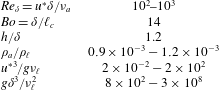
Although the theory derived in this paper is general, quantitative comparison in the following is provided with the only available experimental data of Paquier et al. (Reference Paquier, Moisy and Rabaud2015, Reference Paquier, Moisy and Rabaud2016). We briefly provide here some details about the experiment, and summarise the relevant non-dimensional numbers in table 1.
The experimental set-up consists in a rectangular tank filled with liquid, fitted to the bottom of a wind tunnel of rectangular cross-section. The tank is of length
 $L=1.5~\text{m}$
, width 296 mm, and depth
 $h=35~\text{mm}$
and the channel height is 105 mm. Air (density
 $\unicode[STIX]{x1D70C}_{a}\simeq 1.2~\text{kg}~\text{m}^{-3}$
, kinematic viscosity
 $\unicode[STIX]{x1D708}_{a}\simeq 15\times 10^{-6}~\text{m}^{2}~\text{s}^{-1}$
) is injected at a mean velocity
 $U_{a}$
in the range
 $1{-}10~\text{m}~\text{s}^{-1}$
. The velocity profile in the air is close to that of a classical turbulent boundary layer developing over a no-slip flat wall, at least in the wrinkle regime. The boundary-layer thickness
 $\unicode[STIX]{x1D6FF}$
, defined as the distance from the surface at which the mean velocity is
 $0.99U_{a}$
, is
 $\unicode[STIX]{x1D6FF}\simeq 13~\text{mm}$
at
 $x=0$
, and increases linearly along the tank, with
 $\text{d}\unicode[STIX]{x1D6FF}/\text{d}x\simeq 0.02$
. At the fetch
 $x$
at which the measurements are performed, the local boundary-layer thickness is
 $\unicode[STIX]{x1D6FF}\simeq 30~\text{mm}$
. The friction velocity
 $u^{\ast }$
, determined from measurement of the surface drift velocity using stress continuity, is approximately
 $u^{\ast }\simeq 0.05U_{a}$
.
The liquid viscosity is varied in a wide range,
 $\unicode[STIX]{x1D708}_{\ell }=0.9{-}560\times 10^{-6}~\text{m}^{2}~\text{s}^{-1}$
, using mixtures of glycerol and water (for low
 $\unicode[STIX]{x1D708}_{\ell }$
) or glucose syrup and water (for large
 $\unicode[STIX]{x1D708}_{\ell }$
). The liquid density
 $\unicode[STIX]{x1D70C}_{\ell }$
of the mixtures is in the range
 $1.0{-}1.36\times 10^{3}~\text{kg}~\text{m}^{-3}$
. The surface tension is
 $\unicode[STIX]{x1D6FE}\simeq 60~\text{mN}~\text{m}^{-1}$
, and the capillary length
 $\ell _{c}=\sqrt{\unicode[STIX]{x1D6FE}/\unicode[STIX]{x1D70C}_{\ell }g}$
is approximately 2.2 mm.
For a laminar flow in the liquid, the drift velocity at the surface is given by the continuity of the shear stress, namely
 $U_{s}=\unicode[STIX]{x1D70C}_{a}u^{\ast 2}h/(4\unicode[STIX]{x1D70C}_{\ell }\unicode[STIX]{x1D708}_{\ell })$
. For liquid viscosity
 $\unicode[STIX]{x1D708}_{\ell }>4\unicode[STIX]{x1D708}_{water}$
, the maximum drift velocity in the wrinkle regime is
 $U_{s}\simeq 10~\text{cm}~\text{s}^{-1}$
(for a wind velocity
 $U_{a}\simeq 4.5~\text{m}~\text{s}^{-1}$
), for which the flow in the liquid remains essentially laminar (
 $U_{s}h/\unicode[STIX]{x1D708}_{\ell }<10^{3}$
). For the largest liquid viscosity,
 $\unicode[STIX]{x1D708}_{\ell }\simeq 600\unicode[STIX]{x1D708}_{water}$
, the surface drift does not exceed
 $1~\text{mm}~\text{s}^{-1}$
even at the largest wind velocity, and can be safely neglected. However, for water and liquids of viscosity up to
 $\simeq 4\unicode[STIX]{x1D708}_{water}$
, the drift velocity is significant and the flow in the liquid is no longer laminar. For the sake of simplicity, the effects of the drift velocity and of turbulence in the liquid are not considered in the present paper.
The instantaneous surface deformation fields
 $\unicode[STIX]{x1D701}(\boldsymbol{r},t)$
are measured using free-surface synthetic schlieren (Moisy, Rabaud & Salsac Reference Moisy, Rabaud and Salsac2009). This optical method is based on the analysis of the refracted image of a pattern visualised through the interface. The field of view is
 $390\times 280~\text{mm}$
. The horizontal resolution is 3 mm, and the vertical resolution is
 $0.6~\unicode[STIX]{x03BC}\text{m}$
. The root-mean-square (r.m.s.) wrinkle amplitude is in the range
 $1{-}10~\unicode[STIX]{x03BC}\text{m}$
(
 $\unicode[STIX]{x1D701}_{rms}/\unicode[STIX]{x1D6FF}\simeq 3\times 10^{-5}-3\times 10^{-4}$
).
Set of non-dimensional numbers in the experiments (Paquier et al. Reference Paquier, Moisy and Rabaud2015, Reference Paquier, Moisy and Rabaud2016).

3 Derivation of the spectral theory
In this section we derive an expression in Fourier space relating the surface displacement for arbitrary pressure and shear stress fields applied at a liquid interface from the upper gas phase.
3.1 Assumptions
The calculation is made under the following assumptions:
(i) The gas density is small compared to the liquid density,
 $\unicode[STIX]{x1D70C}_{a}\ll \unicode[STIX]{x1D70C}_{\ell }$
.
(ii) The slope of the surface displacement stays small at all times (
$|\unicode[STIX]{x1D735}\unicode[STIX]{x1D701}|\ll 1$
).(iii) The flow in the liquid is laminar.
(iv) The drift velocity in the liquid is negligible compared to the convection speed of the turbulent structures and the typical phase velocity of the wrinkles.
(v) The liquid layer is of infinite depth.


Assumptions (i)–(iii) are fundamental hypotheses of our theoretical approach. The drift current (assumption (iv)) strongly affects the propagation of surface wave in an oceanographic context (Peregrine Reference Peregrine1976), and correction to the dispersion relation has to be taken into account (Kirby & Chen Reference Kirby and Chen1989; Ellingsen & Li Reference Ellingsen and Li2017). However, in our experimental range of parameters (see § 2.2), the drift current stays within few per cent of the convection speed of the turbulent structures and the typical phase velocity of the wrinkles, so it can be neglected. The finite depth correction (v) will be included in the limit of bulk-dominated dissipation in § 3.4. Two other assumptions shall also be used later but are not required for the following main derivation:
(vi) The surface displacement falls into the propagative wave regime, i.e. the horizontal sizes of the surface displacement are larger than the viscous length
$\ell _{\unicode[STIX]{x1D708}}=g^{-1/3}{\unicode[STIX]{x1D708}_{\ell }}^{2/3}$
.

(vii) The surface displacement
$\unicode[STIX]{x1D701}$
is small compared to the viscous sublayer
$\unicode[STIX]{x1D6FF}_{\unicode[STIX]{x1D708}}$
of the turbulent boundary layer in the air.


Assumption (vi) is comfortably satisfied experimentally in the wrinkle regime for usual values of liquid viscosity,
 $\unicode[STIX]{x1D708}_{\ell }<1000\unicode[STIX]{x1D708}_{water}$
. Assumption (vii) will be useful in § 4 to model the pressure and shear applied at the liquid interface by the gas layer.
3.2 Formulation
We consider a liquid layer submitted to a normal stress field
 $N(x,y,t)$
and a shear stress
 $\boldsymbol{T}(x,y,t)=T_{x}\boldsymbol{e}_{x}+T_{y}\boldsymbol{e}_{y}$
applied at its upper surface in
 $z=\unicode[STIX]{x1D701}(x,y,t)$
. The linearised Navier–Stokes equation for the velocity
 $\boldsymbol{v}=v_{x}\boldsymbol{e}_{x}+v_{y}\boldsymbol{e}_{y}+v_{z}\boldsymbol{e}_{z}$
in the liquid reads
 $$\begin{eqnarray}\displaystyle \unicode[STIX]{x2202}_{t}\boldsymbol{v}=-\frac{1}{\unicode[STIX]{x1D70C}_{\ell }}\unicode[STIX]{x1D735}p_{\ell }+\boldsymbol{g}+\unicode[STIX]{x1D708}_{\ell }\unicode[STIX]{x0394}\boldsymbol{v}, & & \displaystyle\end{eqnarray}$$
where
 $p_{\ell }$
is the pressure in the liquid phase. We have
 $\unicode[STIX]{x1D735}\boldsymbol{\cdot }\boldsymbol{v}=0$
and the boundary condition for an infinite liquid depth reads
 $$\begin{eqnarray}\displaystyle \lim _{z\rightarrow -\infty }\boldsymbol{v}=\mathbf{0}. & & \displaystyle\end{eqnarray}$$
At the interface in
 $z=\unicode[STIX]{x1D701}$
, the continuity condition of the normal stress can be approximated by the pressure in
 $z=0$
using
 $p_{\ell }(x,y,z=\unicode[STIX]{x1D701})=p_{0}-\unicode[STIX]{x1D70C}_{\ell }g\unicode[STIX]{x1D701}$
, where
 $p_{0}=p_{\ell }(x,y,z=0)$
. The continuity condition for the normal stress in
 $z=0$
yields
 $$\begin{eqnarray}\displaystyle p_{0}-\unicode[STIX]{x1D70C}_{\ell }g\unicode[STIX]{x1D701}-2\unicode[STIX]{x1D70C}_{\ell }\unicode[STIX]{x1D708}_{\ell }(\unicode[STIX]{x2202}_{z}v_{z})_{z=0}+\unicode[STIX]{x1D6FE}\unicode[STIX]{x1D6E5}_{(x,y)}\unicode[STIX]{x1D701}=N, & & \displaystyle\end{eqnarray}$$
where
 $\unicode[STIX]{x1D6E5}_{(x,y)}$
is the two-dimensional (2-D) Laplacian. The continuity condition of the tangential stress writes
 $$\begin{eqnarray}\displaystyle & \displaystyle \unicode[STIX]{x1D70C}_{\ell }\unicode[STIX]{x1D708}_{\ell }(\unicode[STIX]{x2202}_{z}v_{x}+\unicode[STIX]{x2202}_{x}v_{z})_{z=0}=T_{x}, & \displaystyle\end{eqnarray}$$
 $$\begin{eqnarray}\displaystyle & \displaystyle \unicode[STIX]{x1D70C}_{\ell }\unicode[STIX]{x1D708}_{\ell }(\unicode[STIX]{x2202}_{z}v_{y}+\unicode[STIX]{x2202}_{y}v_{z})_{z=0}=T_{y}. & \displaystyle\end{eqnarray}$$
3.3 Statistically steady and homogeneous regime
We now look for statistically homogeneous and stationary solutions. We introduce the space–time Fourier transform
 ${\mathcal{F}}$
,
 $$\begin{eqnarray}\displaystyle & \displaystyle \hat{\unicode[STIX]{x1D701}}(\boldsymbol{k},\unicode[STIX]{x1D714})={\mathcal{F}}\{\unicode[STIX]{x1D701}(\boldsymbol{r},t)\}=\int \text{d}^{2}\boldsymbol{r}\,\text{d}t\unicode[STIX]{x1D701}(\boldsymbol{r},t)\text{e}^{-\text{i}(\boldsymbol{k}\boldsymbol{\cdot }\boldsymbol{r}-\unicode[STIX]{x1D714}t)}, & \displaystyle\end{eqnarray}$$
 $$\begin{eqnarray}\displaystyle & \displaystyle \unicode[STIX]{x1D701}(\boldsymbol{r},t)={\mathcal{F}}^{-1}\{\hat{\unicode[STIX]{x1D701}}(\boldsymbol{k},\unicode[STIX]{x1D714})\}=(2\unicode[STIX]{x03C0})^{-3}\int \text{d}^{2}\boldsymbol{k}\,\text{d}\unicode[STIX]{x1D714}\hat{\unicode[STIX]{x1D701}}(\boldsymbol{k},\unicode[STIX]{x1D714})\text{e}^{\text{i}(\boldsymbol{k}\boldsymbol{\cdot }\boldsymbol{r}-\unicode[STIX]{x1D714}t)}, & \displaystyle\end{eqnarray}$$
 $\hat{N}(\boldsymbol{k},\unicode[STIX]{x1D714})$
and
 $\hat{\boldsymbol{T}}(\boldsymbol{k},\unicode[STIX]{x1D714})$
, with
 $\boldsymbol{r}=x\boldsymbol{e}_{x}+y\boldsymbol{e}_{\boldsymbol{y}}$
the horizontal position,
 $\boldsymbol{k}=k_{x}\boldsymbol{e}_{x}+k_{y}\boldsymbol{e}_{y}$
the horizontal wave vector and
 $\unicode[STIX]{x1D714}$
the angular frequency (
 $\boldsymbol{k}$
and
 $\unicode[STIX]{x1D714}$
are real). From (3.1) we obtain
 $$\begin{eqnarray}\displaystyle & \displaystyle \unicode[STIX]{x0394}p_{\ell }=0, & \displaystyle\end{eqnarray}$$
 $$\begin{eqnarray}\displaystyle & \displaystyle \unicode[STIX]{x2202}_{t}\unicode[STIX]{x1D734}-\unicode[STIX]{x1D708}_{\ell }\unicode[STIX]{x0394}\unicode[STIX]{x1D734}=\mathbf{0}, & \displaystyle\end{eqnarray}$$
where we have introduced the vorticity
 $\unicode[STIX]{x1D734}=\unicode[STIX]{x1D735}\times \boldsymbol{v}$
. The boundary conditions for
 $\unicode[STIX]{x1D734}$
write
 $$\begin{eqnarray}\displaystyle & \displaystyle \unicode[STIX]{x1D734}(\boldsymbol{r},z=0,t)=\unicode[STIX]{x1D734}_{0}(\boldsymbol{r},t), & \displaystyle\end{eqnarray}$$
 $$\begin{eqnarray}\displaystyle & \displaystyle \lim _{z\rightarrow -\infty }\unicode[STIX]{x1D734}(\boldsymbol{r},z,t)=\mathbf{0}, & \displaystyle\end{eqnarray}$$
where
 $\unicode[STIX]{x1D734}_{0}(\boldsymbol{r},t)$
is the vorticity at the surface. Equations (3.6) and (3.7) can be solved in Fourier space,
 $$\begin{eqnarray}\displaystyle & \displaystyle p_{\ell }(\boldsymbol{r},z,t)=(2\unicode[STIX]{x03C0})^{-3}\int \text{d}^{2}\boldsymbol{k}\,\text{d}\unicode[STIX]{x1D714}\hat{p}_{0}(\boldsymbol{k},\unicode[STIX]{x1D714})\text{e}^{\text{i}(\boldsymbol{k}\boldsymbol{\cdot }\boldsymbol{r}-\unicode[STIX]{x1D714}t)}\text{e}^{kz}, & \displaystyle\end{eqnarray}$$
 $$\begin{eqnarray}\displaystyle & \displaystyle \unicode[STIX]{x1D734}(\boldsymbol{r},z,t)=(2\unicode[STIX]{x03C0})^{-3}\int \text{d}^{2}\boldsymbol{k}\,\text{d}\unicode[STIX]{x1D714}\hat{\unicode[STIX]{x1D734}}_{0}(\boldsymbol{k},\unicode[STIX]{x1D714})\text{e}^{\text{i}(\boldsymbol{k}\boldsymbol{\cdot }\boldsymbol{r}-\unicode[STIX]{x1D714}t)}\text{e}^{mz}, & \displaystyle\end{eqnarray}$$
where
 $$\begin{eqnarray}\displaystyle m^{2}=k^{2}-\text{i}\unicode[STIX]{x1D714}/\unicode[STIX]{x1D708}_{\ell }, & & \displaystyle\end{eqnarray}$$
with
 $k=(k_{x}^{2}+k_{y}^{2})^{1/2}$
and
 $\{\hat{p}_{0},\hat{\unicode[STIX]{x1D734}}_{0}\}={\mathcal{F}}\{p_{0},\unicode[STIX]{x1D734}_{0}\}$
being the Fourier transforms of the pressure and vorticity at
 $z=0$
. Equation (3.10) shows that an applied pressure patch of typical wavenumber
 $k$
and frequency
 $\unicode[STIX]{x1D714}$
penetrates the liquid layer over a depth
 $k^{-1}$
, while (3.11) shows that the applied shear stress and hence vorticity penetrate over a depth
 $|m|^{-1}$
. These two penetration depths are similar for very viscous fluids, whereas in the limit of low viscosity vorticity remains confined in a thin boundary layer of thickness
 $|m|^{-1}\simeq \sqrt{\unicode[STIX]{x1D708}_{\ell }/\unicode[STIX]{x1D714}}$
.
Rewriting (3.1) as
 $\unicode[STIX]{x2202}_{t}\boldsymbol{v}=-\unicode[STIX]{x1D735}p_{\ell }/\unicode[STIX]{x1D70C}_{\ell }-\unicode[STIX]{x1D708}_{\ell }\unicode[STIX]{x1D735}\times \unicode[STIX]{x1D734}$
, and using (3.10)–(3.11), we obtain the expression of the velocity
 $$\begin{eqnarray}\displaystyle \boldsymbol{v}(\boldsymbol{r},z,t)=(2\unicode[STIX]{x03C0})^{-3}\int \text{d}^{2}\boldsymbol{k}\,\text{d}\unicode[STIX]{x1D714}\left(\frac{\boldsymbol{q}}{\unicode[STIX]{x1D70C}_{\ell }\text{i}\unicode[STIX]{x1D714}}\hat{p}_{0}\text{e}^{kz}+\frac{\unicode[STIX]{x1D708}_{\ell }}{\text{i}\unicode[STIX]{x1D714}}\unicode[STIX]{x1D73F}\times \hat{\unicode[STIX]{x1D734}}_{0}\text{e}^{mz}\right)\text{e}^{\text{i}(\boldsymbol{k}\boldsymbol{\cdot }\boldsymbol{r}-\unicode[STIX]{x1D714}t)}, & & \displaystyle\end{eqnarray}$$
where
 $\boldsymbol{q}=(\text{i}k_{x},\text{i}k_{y},k)$
and
 $\unicode[STIX]{x1D73F}=(\text{i}k_{x},\text{i}k_{y},m)$
. The functions
 $\hat{p}_{0}$
and
 $\hat{\unicode[STIX]{x1D734}}_{0}$
are given by the stress boundary conditions at
 $z=0$
. Combining equations (3.3), (3.4) and (3.13) yields
 $$\begin{eqnarray}\displaystyle & \displaystyle \left(1-\frac{2k^{2}\unicode[STIX]{x1D708}_{\ell }}{\text{i}\unicode[STIX]{x1D714}}\right)\frac{k}{\unicode[STIX]{x1D70C}_{\ell }}\hat{p}_{0}-\frac{2\unicode[STIX]{x1D708}_{\ell }mk}{\text{i}\unicode[STIX]{x1D714}}\unicode[STIX]{x1D708}_{\ell }\hat{B}_{z}-g^{\prime }k\hat{\unicode[STIX]{x1D701}}=\frac{k\hat{N}}{\unicode[STIX]{x1D70C}_{\ell }}, & \displaystyle\end{eqnarray}$$
 $$\begin{eqnarray}\displaystyle & \displaystyle \unicode[STIX]{x1D708}_{\ell }\hat{B}_{z}+2\unicode[STIX]{x1D708}_{\ell }{\mathcal{F}}\{(\unicode[STIX]{x2202}_{zz}v_{z})_{z=0}\}=-\frac{\text{i}\boldsymbol{k}\boldsymbol{\cdot }\hat{\boldsymbol{T}}}{\unicode[STIX]{x1D70C}_{\ell }}, & \displaystyle\end{eqnarray}$$
where
 $g^{\prime }=g+\unicode[STIX]{x1D6FE}k^{2}/\unicode[STIX]{x1D70C}_{\ell }$
is the modified gravity and
 $\hat{B}_{z}=(\unicode[STIX]{x1D73F}\times \hat{\unicode[STIX]{x1D734}}_{0}(\boldsymbol{k},\unicode[STIX]{x1D714}))\boldsymbol{\cdot }\boldsymbol{e}_{z}$
satisfies
 $\unicode[STIX]{x0394}v_{z}=-B_{z}$
. The component
 $B_{z}$
is associated with the viscous dissipation of the vertical component
 $v_{z}$
of the velocity field. Using the kinematic condition
 $\unicode[STIX]{x2202}_{t}\unicode[STIX]{x1D701}=(v_{z})_{z=\unicode[STIX]{x1D701}}$
in the small perturbation limit, we obtain the relation between
 $\hat{\unicode[STIX]{x1D701}},\hat{p}_{0}$
and
 $\hat{B}_{z}$
,
 $$\begin{eqnarray}\displaystyle \unicode[STIX]{x1D714}^{2}\hat{\unicode[STIX]{x1D701}}=\frac{k}{\unicode[STIX]{x1D70C}_{\ell }}\hat{p}_{0}+\unicode[STIX]{x1D708}_{\ell }\hat{B}_{z}, & & \displaystyle\end{eqnarray}$$
where
 $\hat{p}_{0}$
and
 $\hat{B}_{z}$
can be expressed using (3.14) and (3.15). From (3.14), (3.15) and (3.16) we obtain by algebraic manipulations (see details in appendix A) the following expression
 $$\begin{eqnarray}\displaystyle (\unicode[STIX]{x1D714}^{2}-g^{\prime }k+4\text{i}\unicode[STIX]{x1D708}_{\ell }\unicode[STIX]{x1D714}k^{2}+4\unicode[STIX]{x1D708}_{\ell }^{2}k^{3}(m-k))\hat{\unicode[STIX]{x1D701}}=\frac{k\hat{N}}{\unicode[STIX]{x1D70C}_{\ell }}+\frac{m-k}{m+k}\frac{\text{i}\boldsymbol{k}\boldsymbol{\cdot }\hat{\boldsymbol{T}}}{\unicode[STIX]{x1D70C}_{\ell }}. & & \displaystyle\end{eqnarray}$$
We obtain a damped wave equation forced by the normal and tangential stresses applied at the interface. It describes the response of a viscous liquid forced by arbitrary normal and tangential stress fields under the assumptions (i)–(v), in statistically steady and homogeneous configurations. Setting
 $N=0$
and
 $\boldsymbol{T}=\mathbf{0}$
yields the usual dispersion relation for gravity–capillary waves with viscosity (Lamb Reference Lamb1995). In a very viscous fluid (
 $m\simeq k$
), the effect of the shear stress on the flow vanishes, whereas for a fluid of low viscosity (
 $|m|\gg k$
), the effects of pressure and shear stress are comparable. Note here the specificity of the limit
 $\unicode[STIX]{x1D708}_{\ell }\rightarrow 0$
: although
 $(m-k)/(m+k)\rightarrow 1$
, only pressure can generate waves since the inviscid limit implies
 $\boldsymbol{T}=\mathbf{0}$
by tangential stress continuity.
Equation (3.17) can be simplified using the small viscosity approximation (assumption (vi)). The boundary-layer thickness associated with the vertical diffusion of a shear stress patch applied during a time
 $\unicode[STIX]{x1D714}^{-1}$
is
 $\unicode[STIX]{x1D6FF}_{\ell }=\sqrt{\unicode[STIX]{x1D708}_{\ell }/\unicode[STIX]{x1D714}}$
. For a gravity wave of frequency
 $\unicode[STIX]{x1D714}=\sqrt{gk}$
we have
 $\unicode[STIX]{x1D6FF}_{\ell }=\ell _{\unicode[STIX]{x1D708}}^{3/4}k^{-1/4}$
, where
 $\ell _{\unicode[STIX]{x1D708}}=(\unicode[STIX]{x1D708}_{\ell }^{2}/g)^{1/3}$
is the viscous length introduced in § 2.1. In practice,
 $\unicode[STIX]{x1D6FF}_{\ell }$
lies in the range 0.2–7 mm for a typical wrinkle wavelength
 $2\unicode[STIX]{x03C0}/k\approx 100~\text{mm}$
. The thin boundary-layer approximation (vi) is therefore fulfilled. In this limit, we have
 $|m|\gg k$
, and only the first order in
 $\unicode[STIX]{x1D708}_{\ell }$
contributes in (3.17), yielding
 $$\begin{eqnarray}\displaystyle \hat{\unicode[STIX]{x1D701}}(\boldsymbol{k},\unicode[STIX]{x1D714})=\frac{1}{\unicode[STIX]{x1D70C}_{\ell }}\frac{k\hat{N}+\text{i}\boldsymbol{k}\boldsymbol{\cdot }\hat{\boldsymbol{T}}}{\unicode[STIX]{x1D714}^{2}-g^{\prime }k+4\text{i}\unicode[STIX]{x1D708}_{\ell }\unicode[STIX]{x1D714}k^{2}}. & & \displaystyle\end{eqnarray}$$
Equation (3.18) is the corner stone of this paper: it relates the Fourier component of the displacement field
 $\hat{\unicode[STIX]{x1D701}}(\boldsymbol{k},\unicode[STIX]{x1D714})$
to the Fourier components of the applied normal and tangential stresses
 $\hat{N}$
and
 $\hat{\boldsymbol{T}}$
. The surface response in the physical space is finally obtained by applying the inverse Fourier transform (3.5b
) to (3.18),
 $$\begin{eqnarray}\displaystyle \unicode[STIX]{x1D701}(\boldsymbol{r},t)=\frac{1}{(2\unicode[STIX]{x03C0})^{3}}\frac{1}{\unicode[STIX]{x1D70C}_{\ell }}\int \text{d}^{2}\boldsymbol{k}\,\text{d}\unicode[STIX]{x1D714}\frac{k\hat{N}+\text{i}\boldsymbol{k}\boldsymbol{\cdot }\hat{\boldsymbol{T}}}{\unicode[STIX]{x1D714}^{2}-g^{\prime }k+4\text{i}\unicode[STIX]{x1D708}_{\ell }\unicode[STIX]{x1D714}k^{2}}. & & \displaystyle\end{eqnarray}$$
In the specific case of
 $\hat{\boldsymbol{T}}(\boldsymbol{k},\unicode[STIX]{x1D714})=\mathbf{0}$
and
 $\hat{N}(\boldsymbol{k},\unicode[STIX]{x1D714})$
in the form
 $\unicode[STIX]{x1D6FF}(\unicode[STIX]{x1D714}-U_{c}k_{x})\hat{{\mathcal{N}}}(\boldsymbol{k})$
, with
 $U_{c}$
the convection velocity of a rigid pressure source of Fourier transform
 $\hat{{\mathcal{N}}}(\boldsymbol{k})$
, this equation reduces to the classical Havelock integral used to describe the far-field wake of a ship (Havelock Reference Havelock1919; Raphaël & de Gennes Reference Raphaël and de Gennes1996).
3.4 Interpretation
Equation (3.18) can be analysed from the point of view of the linear response theory. It can be written in the form
 $$\begin{eqnarray}\displaystyle \hat{\unicode[STIX]{x1D701}}(\boldsymbol{k},\unicode[STIX]{x1D714})=\frac{{\hat{S}}(\boldsymbol{k},\unicode[STIX]{x1D714})}{\hat{D}(\boldsymbol{k},\unicode[STIX]{x1D714})}, & & \displaystyle\end{eqnarray}$$
with the source term defined as
 $$\begin{eqnarray}\displaystyle {\hat{S}}(\boldsymbol{k},\unicode[STIX]{x1D714})=\frac{k\hat{N}+\text{i}\boldsymbol{k}\boldsymbol{\cdot }\hat{\boldsymbol{T}}}{\unicode[STIX]{x1D70C}_{\ell }}, & & \displaystyle\end{eqnarray}$$
and the (inverse) spectral convolution kernel
 $\hat{D}$
as
 $$\begin{eqnarray}\displaystyle \hat{D}(\boldsymbol{k},\unicode[STIX]{x1D714})=\unicode[STIX]{x1D714}^{2}-g^{\prime }k\tanh (kh)+4\text{i}\unicode[STIX]{x1D708}_{\ell }\unicode[STIX]{x1D714}k^{2}. & & \displaystyle\end{eqnarray}$$
The real part of
 $\hat{D}(\boldsymbol{k},\unicode[STIX]{x1D714})=0$
corresponds to the inviscid dispersion relation for gravity–capillary waves, generalised here to arbitrary depth
 $h$
. This generalisation is valid in the limit of bulk-dominated dissipation for small viscosity (assumption (vii)).
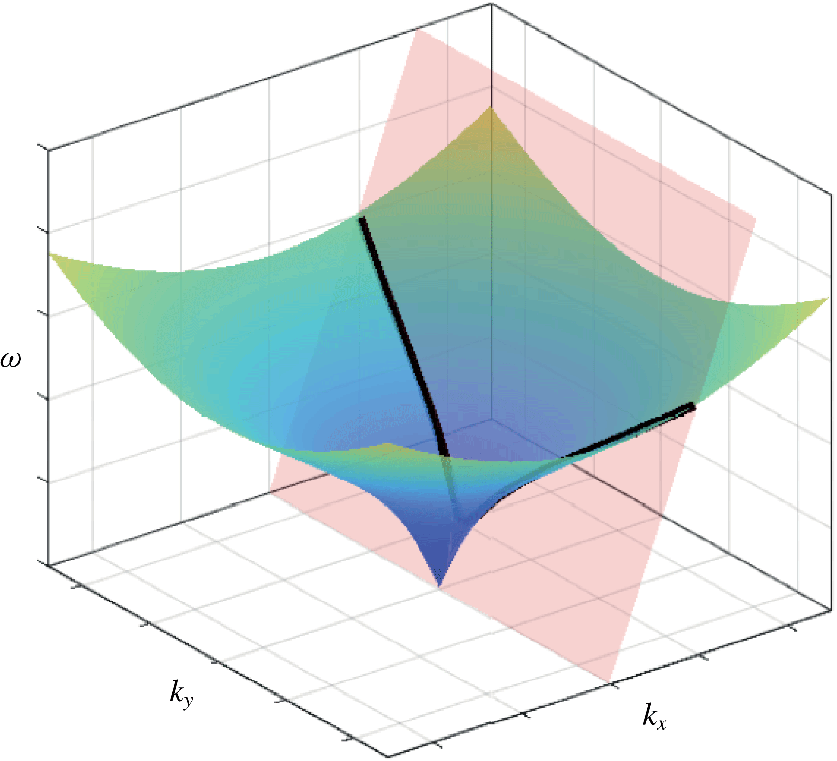
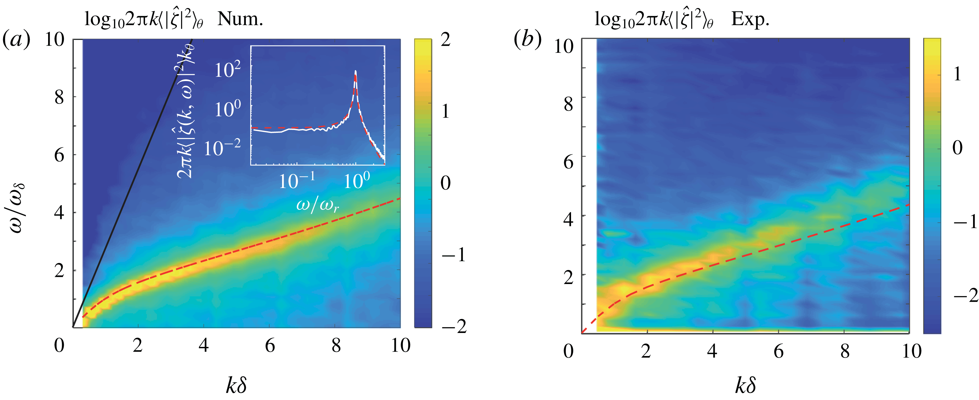
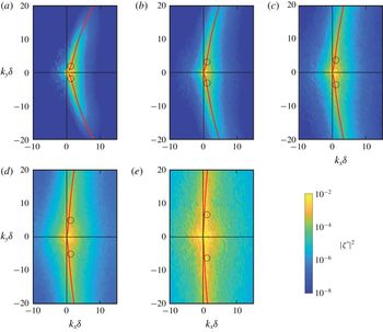
Representation in the Fourier space of the dispersion relation
 $\unicode[STIX]{x1D714}=\sqrt{g^{\prime }k\tanh (kh)}$
of gravity–capillary waves (blue–green surface) and the forcing (pink plane). The forcing here corresponds to a source travelling at constant velocity in the
 $x$
direction,
 $\unicode[STIX]{x1D714}=U_{c}k_{x}$
. The intersection between the two surfaces (black line) is where the maximum wave amplitude is expected.

In the Fourier space
 $(k_{x},k_{y},\unicode[STIX]{x1D714})$
, the inviscid dispersion relation forms a surface with rotational invariance around the
 $\unicode[STIX]{x1D714}$
axis, represented by the blue green surface in figure 2. The Fourier modes
 $(\boldsymbol{k},\unicode[STIX]{x1D714})$
in the immediate vicinity of the surface
 $\hat{D}=0$
correspond to propagative waves. Although the finite depth and the capillary terms are not expected to play a key role in the wrinkle generation (see § 2), we briefly recall here the main properties of the dispersion relation in the general case. Three propagation regimes may be defined:
 $kh\ll 1$
corresponds to the shallow-water regime, in which surface waves are non-dispersive (finite slope at the origin in figure 2, given by the phase velocity
 $c=\unicode[STIX]{x1D714}/k=\sqrt{gh}$
). The two other propagation regimes, lying in the deep-water domain
 $kh\gg 1$
, have a phase velocity
 $c^{2}=g(1/k+k\ell _{c}^{2})$
, with
 $\ell _{c}$
the capillary length. For
 $k\ell _{c}<1$
, gravity effects dominate over capillary forces, while for
 $k\ell _{c}>1$
capillary forces take over, with a change of curvature in
 $\unicode[STIX]{x1D714}$
at
 $k\ell _{c}=1$
. At this inflection point the phase velocity is minimum,
 $c_{min}=(4g\unicode[STIX]{x1D6FE}/\unicode[STIX]{x1D70C}_{\ell })^{1/4}$
. For the interface between air and water or the viscous aqueous solutions considered here, this minimum phase velocity is
 $c_{min}\simeq 22~\text{cm}~\text{s}^{-1}$
.
In view of (3.20), a significant surface response is expected where
 $\hat{D}$
is small and
 ${\hat{S}}$
is large. More specifically, equation (3.20) predicts an excitation of the Fourier modes
 $(\boldsymbol{k},\unicode[STIX]{x1D714})$
supplied by the source
 ${\hat{S}}$
that fall in the vicinity of the dispersion relation. In the simple case of pressure or stress patches rigidly travelling at a constant velocity
 $U_{c}$
in the
 $x$
direction,
 ${\hat{S}}$
is non-zero for
 $\unicode[STIX]{x1D714}=k_{x}U_{c}$
, represented as a tilted plane in pink in figure 2. The intersection between this tilted plane and the surface
 $\hat{D}=0$
(shown as a black curve), which is defined provided that
 $U_{c}\geqslant c_{min}$
, is naturally where wave amplification is expected. For such idealised ‘rigid’ forcing, the resulting wave pattern is a collection of wakes, stationary in the frame of the source (i.e. with a convection velocity given by
 $U_{c}$
), analogous to far-field wakes behind ships.
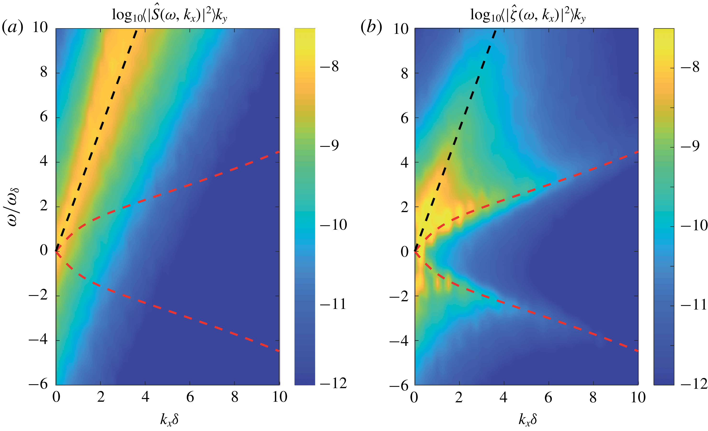
In the case of time-varying forcing, relevant to the problem of a turbulent wind blowing over a liquid surface, the forcing spectrum is now a continuum of Fourier modes centred around
 $\unicode[STIX]{x1D714}\simeq U_{c}k_{x}$
, in a subspace of thickness along
 $\unicode[STIX]{x1D714}$
given by the inverse correlation time of the fluctuations. Loosely speaking, the black line in figure 2 now has a finite thickness, allowing in principle for wave excitation even if
 $U_{c}<c_{min}$
. We expect the wrinkles to be the unstationary wakes generated by this turbulent forcing. For a more quantitative description, the spatio-temporal properties of the forcing
 ${\hat{S}}$
must be specified, to which § 4 is devoted.
It is worth noting that the physical picture given here for the wrinkle regime corresponds only to the linear response of the free surface, and ignores energy transfers between modes of finite amplitude and retroaction on the turbulent forcing. The regular waves, defined as the subset of Fourier modes satisfying
 $k_{y}=0$
(i.e. propagating in the streamwise direction), which are found experimentally at large wind velocity, probably escape from this linear description. Such regular waves first appear with a phase velocity of the order of
 $c_{min}$
, which is much smaller than the forcing velocity
 $U_{c}$
, suggesting that they originate from a retroaction of the liquid surface on the turbulent forcing. We shall return to this point in § 6.2.
3.5 Non-dimensional form
We express now the surface response (3.18) in the form (2.3) inferred from the dimensional analysis. Using the boundary-layer thickness
 $\unicode[STIX]{x1D6FF}$
as the characteristic length and
 $\unicode[STIX]{x1D6FF}/u^{\ast }$
as the characteristic time, we introduce the dimensionless source term
 ${\hat{S}}^{\dagger }$
as
 $$\begin{eqnarray}\displaystyle {\hat{S}}^{\dagger }=\frac{\unicode[STIX]{x1D70C}_{\ell }}{\unicode[STIX]{x1D70C}_{a}}\frac{{\hat{S}}}{u^{\ast }\unicode[STIX]{x1D6FF}^{2}}. & & \displaystyle\end{eqnarray}$$
The mean surface displacement
 $\overline{\unicode[STIX]{x1D701}^{2}}$
can be related to its representation in Fourier space using Parseval’s theorem,
 $$\begin{eqnarray}\displaystyle \int \text{d}^{2}\boldsymbol{r}\,\text{d}t\unicode[STIX]{x1D701}^{2}=\frac{1}{(2\unicode[STIX]{x03C0})^{3}}\int \text{d}^{2}\boldsymbol{k}\,\text{d}\unicode[STIX]{x1D714}|\hat{\unicode[STIX]{x1D701}}|^{2}. & & \displaystyle\end{eqnarray}$$
Replacing
 $\hat{\unicode[STIX]{x1D701}}$
in (3.24) by its expression from (3.20) and (3.23) yields
 $$\begin{eqnarray}\displaystyle \frac{\overline{\unicode[STIX]{x1D701}^{2}}}{\unicode[STIX]{x1D6FF}^{2}}=\left(\frac{\unicode[STIX]{x1D70C}_{a}}{\unicode[STIX]{x1D70C}_{\ell }}\right)^{2}\frac{{u^{\ast }}^{3}}{\unicode[STIX]{x1D6FF}}\frac{1}{(2\unicode[STIX]{x03C0})^{3}}\int \text{d}^{2}\boldsymbol{k}\,\text{d}\unicode[STIX]{x1D714}\frac{|{\hat{S}}^{\dagger }|^{2}}{(\unicode[STIX]{x1D714}^{2}-\unicode[STIX]{x1D714}_{r}^{2})^{2}+\unicode[STIX]{x1D714}_{\unicode[STIX]{x1D708}}^{2}\unicode[STIX]{x1D714}^{2}}, & & \displaystyle\end{eqnarray}$$
where
 $\unicode[STIX]{x1D714}_{r}=\sqrt{g^{\prime }k\tanh (kh)}$
is the surface wave frequency and
 $\unicode[STIX]{x1D714}_{\unicode[STIX]{x1D708}}=4\unicode[STIX]{x1D708}_{\ell }k^{2}$
is the dissipation rate. Equation (3.25) needs further specifications to be written in a dimensionless form. A choice arises for the dimensionless frequency, which can be constructed either from the characteristic time of the source,
 $\unicode[STIX]{x1D6FF}/u^{\ast }$
, or from the characteristic time of the surface response,
 ${\unicode[STIX]{x1D714}_{\unicode[STIX]{x1D708}}}^{-1}$
. We chose the dimensionless frequencies
 $\tilde{\unicode[STIX]{x1D714}}=\unicode[STIX]{x1D714}/\unicode[STIX]{x1D714}_{\unicode[STIX]{x1D708}}$
,
 $\tilde{\unicode[STIX]{x1D714}}_{r}=\unicode[STIX]{x1D714}_{r}/\unicode[STIX]{x1D714}_{\unicode[STIX]{x1D708}}$
and the dimensionless wavenumber
 $\tilde{k}=k\unicode[STIX]{x1D6FF}$
, yielding
 $$\begin{eqnarray}\displaystyle \frac{\overline{\unicode[STIX]{x1D701}^{2}}}{\unicode[STIX]{x1D6FF}^{2}} & = & \displaystyle \left(\frac{\unicode[STIX]{x1D70C}_{a}}{\unicode[STIX]{x1D70C}_{\ell }}\right)^{2}\frac{{u^{\ast }}^{3}}{4g\unicode[STIX]{x1D708}_{\ell }}\frac{1}{(2\unicode[STIX]{x03C0})^{3}}\nonumber\\ \displaystyle & & \displaystyle \times \int \text{d}^{2}\tilde{\boldsymbol{k}}\,\text{d}\tilde{\unicode[STIX]{x1D714}}\frac{1}{\tilde{k}^{3}(1+Bo^{-2}\tilde{k}^{2})\tanh (\tilde{k}h/\unicode[STIX]{x1D6FF})}\frac{|{\hat{S}}^{\dagger }|^{2}}{(\tilde{\unicode[STIX]{x1D714}}-\tilde{\unicode[STIX]{x1D714}}_{r})^{2}(\tilde{\unicode[STIX]{x1D714}}/\tilde{\unicode[STIX]{x1D714}}_{r}+1)^{2}+(\tilde{\unicode[STIX]{x1D714}}/\tilde{\unicode[STIX]{x1D714}}_{r})^{2}}.\qquad \;\;\end{eqnarray}$$
This equation confirms the role played by the dimensionless combination
 ${u^{\ast }}^{3}/(g\unicode[STIX]{x1D708}_{\ell })$
introduced in § 2, and provides an analytical expression for the dimensionless function
 $f_{3}$
in (2.3). However, the dependency in Reynolds number is hidden in the source term
 ${\hat{S}}^{\dagger }$
. Hence, a quantitative description of the spectral source originating from the turbulent boundary layer in the air phase is now required.
4 Properties of the turbulent forcing from DNS
We compute the source term
 ${\hat{S}}$
using a set of time-resolved pressure and shear stress fields evaluated at
 $z=0$
, taken from three-dimensional DNS of a developed turbulent flow in a non-deformable channel with no-slip condition at the bottom and top boundaries, and periodic boundary conditions along the streamwise and spanwise directions. In order to provide comparison with the experiments of Paquier et al. (Reference Paquier, Moisy and Rabaud2015, Reference Paquier, Moisy and Rabaud2016), which were performed in a developing boundary-layer flow, we assume here that the spatio-temporal statistics of turbulence in a developing boundary layer of thickness
 $\unicode[STIX]{x1D6FF}$
at a given
 $Re_{\unicode[STIX]{x1D6FF}}=\unicode[STIX]{x1D6FF}u^{\ast }/\unicode[STIX]{x1D708}_{a}$
are equivalent to those of a channel flow of half-height
 $H$
at the same value of
 $Re_{\unicode[STIX]{x1D70F}}=Hu^{\ast }/\unicode[STIX]{x1D708}_{a}$
. Previous works have shown that this assumption is reasonably well satisfied for the flow close to the wall,
 $z<0.6\unicode[STIX]{x1D6FF}$
(Jimenez & Hoyas Reference Jimenez and Hoyas2008; Jimenez et al.
Reference Jimenez, Hoyas, Simens and Mizuno2010). In the following, we identify
 $H$
to
 $\unicode[STIX]{x1D6FF}$
and we use for simplicity the same notation
 $Re_{\unicode[STIX]{x1D6FF}}$
for the DNS and the experiments.
4.1 Boundary conditions
We first examine to what extent a canonical turbulent flow over a smooth and rigid wall with no-slip boundary condition can adequately model the turbulence over a free surface. We base our analysis of the air flow on three assumptions:
(i) The interface is slightly deformable,
$\unicode[STIX]{x2202}_{t}\unicode[STIX]{x1D701}|_{z=0^{+}}=v_{z}|_{z=0^{+}}\ll v_{x,y}|_{z=0^{+}}$
.(ii) The interface is smooth,
$\unicode[STIX]{x1D701}\ll \unicode[STIX]{x1D6FF}_{\unicode[STIX]{x1D708}}$
.(iii) The surface drift velocity in the liquid is negligible compared to the velocity of the turbulent structures,
$v_{x}|_{z=0^{-}}\ll U_{a}$
.



These three assumptions are corollary of the assumptions (ii), (iv) and (vii) discussed in § 3.1. The rigid wall approximation is equivalent to the linear approximation (ii). The smooth wall approximation is motivated by the typical wrinkle amplitude
 $\unicode[STIX]{x1D701}_{rms}$
, at least ten times smaller than the viscous sublayer
 $\unicode[STIX]{x1D6FF}_{\unicode[STIX]{x1D708}}$
below the wind wave threshold (Paquier et al.
Reference Paquier, Moisy and Rabaud2016). It is therefore a consequence of assumption (vii). Finally, the no-slip boundary condition derives from assumption (iv).
Under these assumptions, we model the turbulence by a turbulent channel flow over a smooth and rigid wall with no-slip boundary condition in
 $z=0$
and
 $z=2H$
and periodic boundary conditions along
 $x$
and
 $y$
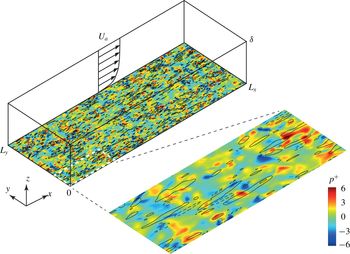
. The DNS configuration is sketched in figure 3, with
 $L_{x},L_{y}$
the streamwise and the spanwise lengths. The flow is driven by a mean streamwise pressure gradient
 $-P_{a}/L_{x}$
. By conservation of the streamwise momentum, the mean tangential stress at the boundaries is
 $\unicode[STIX]{x1D70F}_{a}=HP_{a}/L_{x}$
, which defines the friction velocity
 $u^{\ast }=\sqrt{\unicode[STIX]{x1D70F}_{a}/\unicode[STIX]{x1D70C}_{a}}$
. We decompose the instantaneous pressure at the wall as the sum of a stationary pressure drop
 $P(x)=P_{a}(1-x/L_{x})$
and turbulent pressure fluctuations
 $p(x,y,t)$
of zero mean. Similarly, the wall shear stress is the sum of a stationary component
 $\unicode[STIX]{x1D70F}_{a}\boldsymbol{e}_{\boldsymbol{x}}$
and fluctuations
 $\unicode[STIX]{x1D748}(x,y,t)=\unicode[STIX]{x1D70E}_{x}\boldsymbol{e}_{\boldsymbol{x}}+\unicode[STIX]{x1D70E}_{y}\boldsymbol{e}_{\boldsymbol{y}}$
of zero mean. As argued before, the steady contributions are responsible for a mean flow generation in the liquid, which is not considered here. In the following, we focus on the fluctuating contributions
 $(p,\unicode[STIX]{x1D748})$
.
Sketch of the numerical set-up. The pressure and the shear stress on the wall plane
 $z=0$
taken from DNS of a turbulent channel flow are applied to the surface of a viscous liquid. The DNS is performed in a domain
 $(L_{x},L_{y},L_{z})=(8\unicode[STIX]{x03C0},3\unicode[STIX]{x03C0},2)\unicode[STIX]{x1D6FF}$
. The snapshot illustrates the turbulent field at
 $z=0$
for the case
 $Re_{\unicode[STIX]{x1D6FF}}=250$
. Pressure
 $p^{+}=p/(\unicode[STIX]{x1D70C}_{a}u^{\ast 2})$
is shown in colour, and longitudinal shear stress
 $\unicode[STIX]{x1D70E}_{x}^{+}$
as contour lines (lines are separated by increments
 $\unicode[STIX]{x1D70E}_{x}^{+}=1$
, positive for full lines and negative for dashed lines). A magnification of the snapshot by a factor 4 in each direction is also presented.

To compute the source term
 ${\hat{S}}=(k\hat{N}+\text{i}\boldsymbol{k}\boldsymbol{\cdot }\hat{\boldsymbol{T}})/\unicode[STIX]{x1D70C}_{\ell }$
from the
 $(p,\unicode[STIX]{x1D748})$
, we need to specify the normal and tangential stresses,
 $$\begin{eqnarray}\displaystyle & \displaystyle N=p+2\unicode[STIX]{x1D70C}_{a}\unicode[STIX]{x1D708}_{a}(\unicode[STIX]{x2202}_{z}v_{z})_{|z=0^{+}}, & \displaystyle\end{eqnarray}$$
 $$\begin{eqnarray}\displaystyle & \displaystyle T_{x}=\unicode[STIX]{x1D70E}_{x}+\unicode[STIX]{x1D70C}_{a}\unicode[STIX]{x1D708}_{a}(\unicode[STIX]{x2202}_{x}v_{z})_{|z=0^{+}}, & \displaystyle\end{eqnarray}$$
 $$\begin{eqnarray}\displaystyle & \displaystyle T_{y}=\unicode[STIX]{x1D70E}_{y}+\unicode[STIX]{x1D70C}_{a}\unicode[STIX]{x1D708}_{a}(\unicode[STIX]{x2202}_{y}v_{z})_{|z=0^{+}}. & \displaystyle\end{eqnarray}$$
The relative importance of the viscous contributions depends on the surface deformation and the magnitude of the turbulent air flow. For a surface displacement
 $\unicode[STIX]{x1D701}$
of characteristic wavenumber
 $k$
and convection speed
 $U_{c}$
, spatial gradients of
 $v_{z}$
scale as
 $\unicode[STIX]{x2202}_{x,y,z}v_{z}\approx \unicode[STIX]{x1D701}U_{c}k^{2}$
. For a turbulent boundary layer of friction velocity
 $u^{\ast }$
, the vertical gradient of horizontal velocity scales as
 $\unicode[STIX]{x2202}_{z}v_{x,y}\approx u^{\ast }/\unicode[STIX]{x1D6FF}_{\unicode[STIX]{x1D708}}$
. The ratio
 $\unicode[STIX]{x2202}_{x,y}v_{z}/\unicode[STIX]{x2202}_{z}v_{x,y}$
is thus given by
 $\unicode[STIX]{x1D701}\unicode[STIX]{x1D6FF}_{\unicode[STIX]{x1D708}}u^{\ast }k^{2}/U_{c}$
, where
 $U_{c}\approx 12u^{\ast }$
. If we consider a wave of wavelength
 $\unicode[STIX]{x1D6EC}$
, using assumption (ii),
 $\unicode[STIX]{x1D701}\ll \unicode[STIX]{x1D6EC}$
, and assumption (vii),
 $\unicode[STIX]{x1D6FF}_{\unicode[STIX]{x1D708}}\ll \unicode[STIX]{x1D6EC}$
, we have in practice
 $\unicode[STIX]{x2202}_{x,y,z}v_{z}\ll \unicode[STIX]{x2202}_{z}v_{x,y}$
in the wrinkle regime. The expressions of
 $N$
and
 $\boldsymbol{T}$
thus reduce to
 $$\begin{eqnarray}\displaystyle & \displaystyle N=p, & \displaystyle\end{eqnarray}$$
 $$\begin{eqnarray}\displaystyle & \displaystyle \boldsymbol{T}=\unicode[STIX]{x1D748}, & \displaystyle\end{eqnarray}$$
where
 $p$
is the air pressure and
 $\unicode[STIX]{x1D748}$
is the tangential wall stress in the limit of a non-deformable wall. In the following, we use the conventional wall-unit notation
 $+$
,
 $$\begin{eqnarray}\displaystyle \{p,\unicode[STIX]{x1D748}\}=\unicode[STIX]{x1D70C}_{a}{u^{\ast }}^{2}\{p^{+},\unicode[STIX]{x1D748}^{+}\}, & & \displaystyle\end{eqnarray}$$
so the dimensionless source term
 ${\hat{S}}^{\dagger }$
defined in (3.23) reads
 $$\begin{eqnarray}\displaystyle {\hat{S}}^{\dagger }(\boldsymbol{k},\unicode[STIX]{x1D714})=\tilde{k}\hat{p}^{+}+\text{i}\tilde{\boldsymbol{k}}\boldsymbol{\cdot }\hat{\unicode[STIX]{x1D748}}^{+}, & & \displaystyle\end{eqnarray}$$
with
 $\tilde{\boldsymbol{k}}=\boldsymbol{k}\unicode[STIX]{x1D6FF}$
.
4.2 DNS configuration
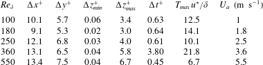
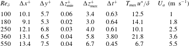
Details of the DNS turbulent channel flow:
 $\unicode[STIX]{x0394}x^{+}$
and
 $\unicode[STIX]{x0394}y^{+}$
are the spatial resolutions in terms of Fourier modes before dealiasing;
 $\unicode[STIX]{x0394}z_{min}^{+}$
and
 $\unicode[STIX]{x0394}z_{max}^{+}$
are the finest and coarsest spatial resolutions in the wall-normal direction in dimensionless units;
 $\unicode[STIX]{x0394}t^{+}$
is the temporal separation between stored flow fields and
 $T_{max}$
is the total time simulated;
 $U_{a}$
is the corresponding wind velocity for a boundary-layer thickness
 $\unicode[STIX]{x1D6FF}\simeq 30~\text{mm}$
and a kinematic viscosity of air
 $\unicode[STIX]{x1D708}_{a}=15\times 10^{-6}~\text{m}^{2}~\text{s}^{-1}$
(see § 2.2).
The numerical set-up is sketched in figure 3, with the wall pressure and wall shear stress taken for
 $Re_{\unicode[STIX]{x1D6FF}}=250$
. The parameters for each DNS run are summarised in table 2. The turbulent Reynolds number
 $Re_{\unicode[STIX]{x1D6FF}}$
ranges from 100 to 550, which corresponds in the experiments of Paquier et al. (Reference Paquier, Moisy and Rabaud2015) to wind speeds ranging from 1 to
 $5.5~\text{m}~\text{s}^{-1}$
. This correspondence is obtained by equating the DNS and experimental values of
 $Re_{\unicode[STIX]{x1D6FF}}$
, with
 $\unicode[STIX]{x1D708}_{a}=15\times 10^{-6}~\text{m}~\text{s}^{-2}$
for the kinematic viscosity of air, and
 $\unicode[STIX]{x1D6FF}\simeq 30~\text{mm}$
for the local boundary-layer thickness at the
 $x$
-location where measurements are carried out (see § 2.2).
The incompressible flow is integrated in the form of evolution equations for the wall-normal vorticity and for the Laplacian of the wall-normal velocity, as in Kim, Moin & Moser (Reference Kim, Moin and Moser1987), and the spatial discretisation is desaliased Fourier series in the two wall-parallel directions and Chebyshev polynomials in
 $z$
. Time stepping is the third-order semi-implicit Runge–Kutta method from Moser et al. (Reference Moser, Kim and Mansour1999).
The computational box is
 $L_{x}\times L_{y}\times L_{z}=(8\unicode[STIX]{x03C0},3\unicode[STIX]{x03C0},2)\unicode[STIX]{x1D6FF}$
with periodic boundary conditions along
 $x$
and
 $y$
directions. These spatial dimensions are larger than the minimum channel size
 $(2\unicode[STIX]{x03C0},\unicode[STIX]{x03C0},2)\unicode[STIX]{x1D6FF}$
often used in numerical simulation (Jimenez Reference Jimenez2013). Preliminary tests showed that this large domain size is necessary to ensure the correct convergence of the Fourier integral (3.19), which is dominated by the contributions at small
 $\boldsymbol{k}$
.
The periodic boundary condition in time, implicitly assumed in our spectral formulation, is naturally not satisfied in the DNS data. However, spurious temporal correlations are limited by the large computational domain: the correlation time of the pressure fluctuations, of the order of
 $20Re_{\unicode[STIX]{x1D6FF}}^{-1}\unicode[STIX]{x1D6FF}/u^{\ast }$
, is comfortably smaller than the transit time over the computational domain, of the order of
 $L_{x}/U_{c}\simeq 2\unicode[STIX]{x1D6FF}/u^{\ast }$
, where
 $U_{c}$
is the convection velocity (see § 4.3). The total integration time
 $T_{max}$
is chosen to be at least
 $10\unicode[STIX]{x1D6FF}/u^{\ast }$
(except for the largest
 $Re_{\unicode[STIX]{x1D6FF}}$
), to correctly resolve the lowest frequencies
 $\unicode[STIX]{x1D714}$
in the wave dynamics. The time step,
 $\unicode[STIX]{x0394}t^{+}$
, is sufficiently small to resolve the fastest waves (the case
 $Re_{\unicode[STIX]{x1D6FF}}=360$
has a coarser time step in order to collect statistics for a longer time period).
4.3 Pressure and shear stress statistics at the wall
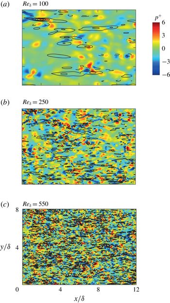
Snapshots of the pressure and shear stress fields at the surface, at three values of
 $Re_{\unicode[STIX]{x1D6FF}}$
. Only a subdomain
 $[0,12\unicode[STIX]{x1D6FF}]\times [0,8\unicode[STIX]{x1D6FF}]$
is shown. The pressure
 $p^{+}=p/(\unicode[STIX]{x1D70C}_{a}u^{\ast 2})$
is shown in colour, and the longitudinal shear stress
 $\unicode[STIX]{x1D70E}_{x}^{+}$
as contour lines, such that
 $|\unicode[STIX]{x1D70E}_{x}^{+}|=0.5i$
with integer
 $i$
(positive for full lines and negative for dashed lines).

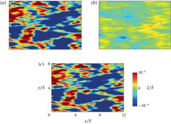
Figure 4 shows snapshots of the instantaneous wall pressure
 $p^{+}$
and streamwise wall shear stress
 $\unicode[STIX]{x1D70E}_{x}^{+}$
for Reynolds numbers
 $Re_{\unicode[STIX]{x1D6FF}}=100,250$
and 550. Increasing the Reynolds number naturally decreases the size of the structures. These snapshots show that the shear stress patterns tend to be elongated in the streamwise direction, whereas the pressure patterns are nearly isotropic in the
 $(x,y)$
plane. These elongated shear stress patterns are a classic signature of the streamwise streaks in the near-wall region of the boundary layer, whereas the nearly isotropic pressure patterns are related to the imprint created at the wall by the cores of the vortices (Jimenez Reference Jimenez2013).
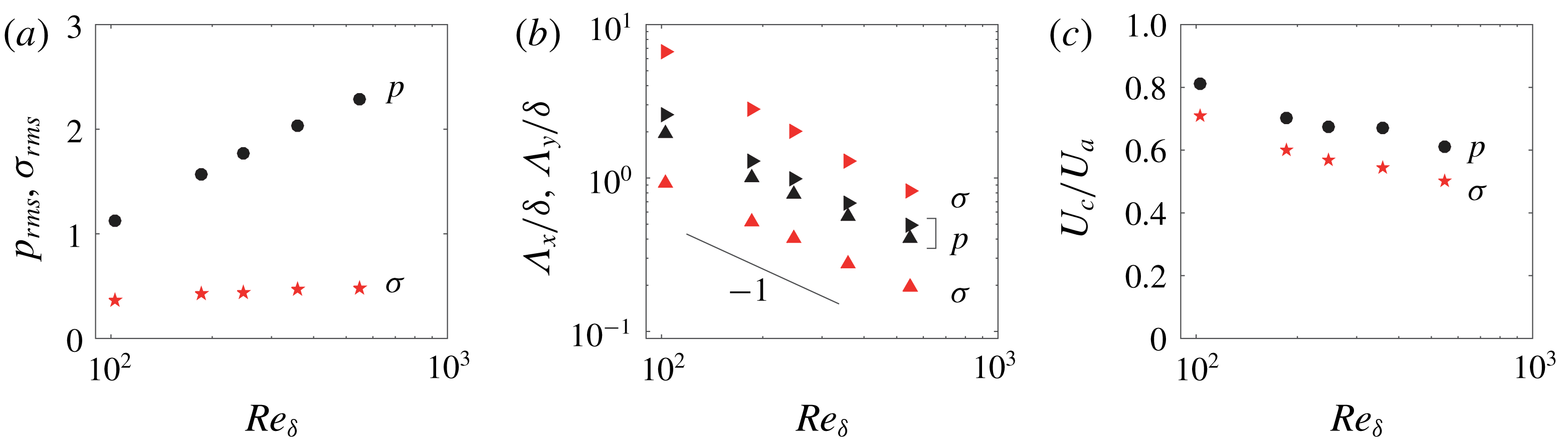
Statistics of pressure and shear stress fluctuations as a function of
 $Re_{\unicode[STIX]{x1D6FF}}$
. (a) Root-mean-squared pressure
 $p_{rms}^{+}$
(●) and stress
 $\unicode[STIX]{x1D70E}_{rms}^{+}=({{\unicode[STIX]{x1D70E}_{x}^{+}}_{rms}}^{2}+{{\unicode[STIX]{x1D70E}_{y}^{+}}_{rms}}^{2})^{1/2}$
(
 $\star$
). (b) Characteristic streamwise and spanwise lengths
 $\unicode[STIX]{x1D6EC}_{x}/\unicode[STIX]{x1D6FF}$
(▸, ▸ red) and
 $\unicode[STIX]{x1D6EC}_{y}/\unicode[STIX]{x1D6FF}$
(▴, ▴ red) of pressure and shear stress, computed from the spectral barycentres (4.8); for
 $\unicode[STIX]{x1D70E}$
, the values of
 $\unicode[STIX]{x1D6EC}$
are averaged over the two components
 $\unicode[STIX]{x1D70E}_{x}$
and
 $\unicode[STIX]{x1D70E}_{y}$
. Structure sizes decrease as
 $\unicode[STIX]{x1D6EC}\propto Re_{\unicode[STIX]{x1D6FF}}^{-1}$
(black solid line). (c) Mean convection velocity
 $U_{c}/U_{a}$
for pressure (●) and shear stress (
 $\star$
), computed using (4.10).

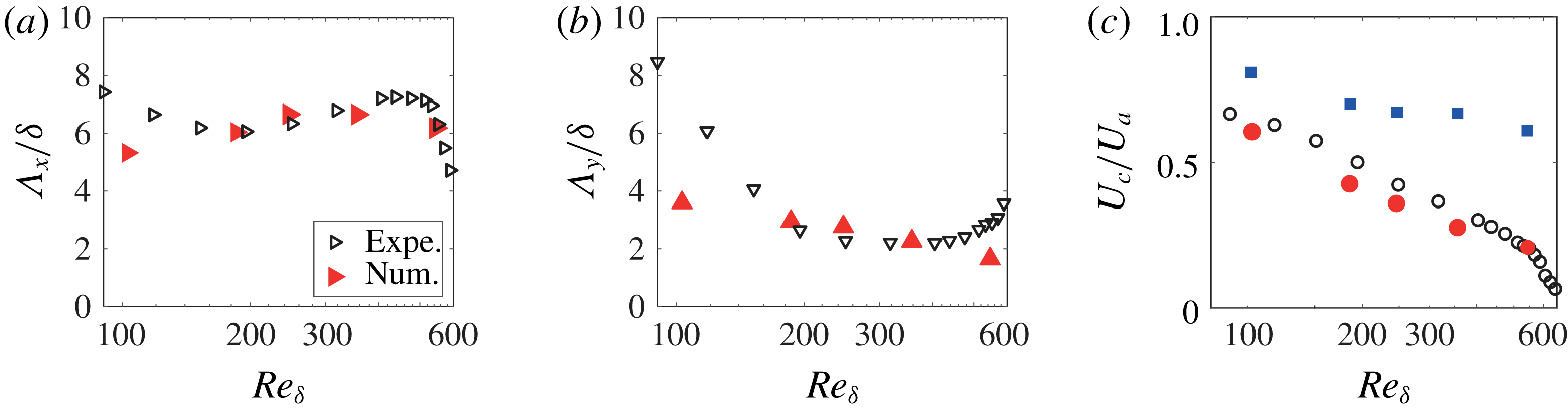
The intensities and sizes of the pressure and shear stress fluctuations are quantified in figure 5 as a function of the Reynolds number. The pressure r.m.s. (figure 5
a) is typically 2 to 5 times larger than the shear stress r.m.s. and increases weakly with
 $Re_{\unicode[STIX]{x1D6FF}}$
, while the shear stress r.m.s. remains nearly constant over the range of
 $Re_{\unicode[STIX]{x1D6FF}}$
considered. We can therefore anticipate that the surface response will be dominated by the pressure forcing.
To compute the characteristic dimensions of the pressure and shear stress structures, we define for any field
 $f(\boldsymbol{r},t)$
the spectral barycentre
 $\boldsymbol{K}$
,
 $$\begin{eqnarray}\displaystyle \boldsymbol{K}=K_{x}\boldsymbol{e}_{\boldsymbol{x}}+K_{y}\boldsymbol{e}_{\boldsymbol{y}}=\frac{\displaystyle \int _{{\mathcal{D}}}\text{d}^{2}\boldsymbol{k}\,\text{d}\unicode[STIX]{x1D714}\boldsymbol{k}|\hat{f}|^{2}}{\displaystyle \int _{{\mathcal{D}}}\text{d}^{2}\boldsymbol{k}\,\text{d}\unicode[STIX]{x1D714}|\hat{f}|^{2}}, & & \displaystyle\end{eqnarray}$$
where
 $\hat{f}(\boldsymbol{k},\unicode[STIX]{x1D714})$
is the Fourier transform of
 $f$
, and
 ${\mathcal{D}}=\{(k_{x},k_{y},\unicode[STIX]{x1D714})|k_{x}>0,k_{y}>0\}$
is the domain of integration. The mean structure sizes in the streamwise and spanwise directions, defined as
 $\unicode[STIX]{x1D6EC}_{x}=2\unicode[STIX]{x03C0}/K_{x}$
and
 $\unicode[STIX]{x1D6EC}_{y}=2\unicode[STIX]{x03C0}/K_{y}$
, are plotted in figure 5(b) for the pressure and the shear stress;
 $\unicode[STIX]{x1D6EC}_{x}$
and
 $\unicode[STIX]{x1D6EC}_{y}$
both decrease as
 $Re_{\unicode[STIX]{x1D6FF}}^{-1}$
, indicating that they scale as the (inner) viscous sublayer thickness
 $\unicode[STIX]{x1D6FF}_{\unicode[STIX]{x1D708}}$
. The sizes are normalised by
 $\unicode[STIX]{x1D6FF}_{\unicode[STIX]{x1D708}}$
are
 $\unicode[STIX]{x1D6EC}_{x}^{+}\simeq \unicode[STIX]{x1D6EC}_{y}^{+}\simeq 250$
for the pressure patches, and
 $\unicode[STIX]{x1D6EC}_{x}^{+}\simeq 700$
,
 $\unicode[STIX]{x1D6EC}_{y}^{+}\simeq 100$
for the shear stress patches.
Similarly, we can define the frequency barycentre
 $\unicode[STIX]{x1D6FA}$
of a field
 $f$
as
 $$\begin{eqnarray}\displaystyle \unicode[STIX]{x1D6FA}=\frac{\displaystyle \int _{{\mathcal{D}}}\text{d}^{2}\boldsymbol{k}\,\text{d}\unicode[STIX]{x1D714}\unicode[STIX]{x1D714}|\hat{f}|^{2}}{\displaystyle \int _{{\mathcal{D}}}\text{d}^{2}\boldsymbol{k}\,\text{d}\unicode[STIX]{x1D714}|\hat{f}|^{2}}. & & \displaystyle\end{eqnarray}$$
We finally define the convection velocity
 $U_{c}$
as
 $$\begin{eqnarray}\displaystyle U_{c}=\unicode[STIX]{x1D6FA}/K_{x}. & & \displaystyle\end{eqnarray}$$
The convection velocity
 $U_{c}$
for the pressure and the shear stress, plotted in figure 5(c), lies in the range
 $[0.5,0.8]U_{a}$
. It slightly decreases with
 $Re_{\unicode[STIX]{x1D6FF}}$
, down to
 $U_{c}\approx 0.6U_{a}$
for the pressure and
 $0.5U_{a}$
for the shear stress. These values correspond to the mean velocity at the wall-normal location
 $z^{+}\simeq 30$
where the turbulent fluctuations are maximum (Kim Reference Kim1989). Note however that this convection velocity is an average over Fourier components traveling at different velocities: the largest structures propagate at
 $U_{c}\approx 0.8U_{a}$
while the small-scale structures propagate at a slightly lower value,
 $U_{c}\approx 0.6U_{a}$
, as observed experimentally (Willmarth & Wooldridge Reference Willmarth and Wooldridge1962; Corcos Reference Corcos1963) and numerically (Choi & Moin Reference Choi and Moin1990).
5 Integrated model of the wrinkle regime
We now combine the analytical results for the surface response (§ 3) with the DNS of the turbulent boundary layer (§ 4) to determine the statistical properties of the wrinkles. We first compute in § 5.1 the spatio-temporal fields of synthetic wrinkles from direct integration of (3.19) using three-dimensional discrete Fourier transform, and compare them to experimental data. Although a good qualitative agreement is obtained, this direct method suffers from discretisation effects at small wavenumber. To circumvent this difficulty, we analyse the surface response in the spectral space in § 5.2, and we introduce in § 5.3 a semi-analytical method to evaluate the three-dimensional integral from its dominant contribution in the vicinity of the two-dimensional resonant manifold. This method gives more insight into the physics of the wrinkles and their scaling properties.
5.1 Surface displacement computation
We first provide here a direct computation of time series of synthetic wrinkles fields from direct integration of (3.19). From the space–time Fourier transform of the wall pressure
 $\hat{p}^{+}(\boldsymbol{k},\unicode[STIX]{x1D714})$
and wall shear stress
 $\hat{\unicode[STIX]{x1D748}}^{+}(\boldsymbol{k},\unicode[STIX]{x1D714})$
extracted from the DNS runs, we compute the source term
 ${\hat{S}}^{\dagger }(\boldsymbol{k},\unicode[STIX]{x1D714})$
from (4.7) on a discrete three-dimensional Cartesian grid
 $(k_{x},k_{y},\unicode[STIX]{x1D714})$
. Since the surface response occurs mainly at low wavenumber and low frequency, we perform a spectral decimation: we retain only the modes
 $k_{i}\unicode[STIX]{x1D6FF}<20$
and
 $\unicode[STIX]{x1D714}\unicode[STIX]{x1D6FF}/U_{a}<25$
.
Comparison between experimental surface displacement field
 $\unicode[STIX]{x1D701}$
measured by Paquier et al. (Reference Paquier, Moisy and Rabaud2015) (a,c,e) and synthetic wrinkle fields computed from DNS data with (3.19) (b,d,f). Only a subdomain of the synthetic wrinkle field is shown, to match the size of the experimental domain. Experimental data (a,c,e) for
 $U_{a}=1~\text{m}~\text{s}^{-1}$
(a),
 $2.5~\text{m}~\text{s}^{-1}$
(c) and
 $5.5~\text{m}~\text{s}^{-1}$
(e), which correspond to
 $Re_{\unicode[STIX]{x1D6FF}}=100$
(b),
 $Re_{\unicode[STIX]{x1D6FF}}=250$
(d),
 $Re_{\unicode[STIX]{x1D6FF}}=550$
(f).

Figure 6 shows snapshots of synthetic wrinkle fields computed using this direct method, for
 $Re_{\unicode[STIX]{x1D6FF}}=100,250$
and 550, compared to experimental measurements by Paquier et al. (Reference Paquier, Moisy and Rabaud2015) for a liquid viscosity
 $\unicode[STIX]{x1D708}_{\ell }=30~\text{mm}^{2}~\text{s}^{-1}$
and equivalent Reynolds numbers (the corresponding wind speeds are
 $U_{a}=1$
, 2.5 and
 $5.5~\text{m}~\text{s}^{-1}$
). These synthetic fields are obtained from the pressure and shear stress snapshots shown in figure 4. The wrinkles appear as disordered fluctuations, nearly isotropic at
 $Re_{\unicode[STIX]{x1D6FF}}=100$
, that become elongated in the streamwise direction as
 $Re_{\unicode[STIX]{x1D6FF}}$
increases. We can note the good qualitative agreement between experimental and synthetic wrinkles for
 $Re_{\unicode[STIX]{x1D6FF}}=100$
and 250 (quantitative comparisons are provided in § 5.3). By comparing figures 4 and 6, we note that the characteristic size of the wrinkles is always significantly larger than the size of the pressure and shear stress pattern from which they originate. This shift of the surface response towards larger scales is a key feature of the wrinkle regime. More precisely, the width of the wrinkles slightly decreases with
 $Re_{\unicode[STIX]{x1D6FF}}$
, while their length remains nearly constant. The match between experimental and synthetic wrinkles is not as good at larger Reynolds number, for
 $Re_{\unicode[STIX]{x1D6FF}}=550$
: as the Reynolds number is increased, the DNS resolves smaller scales, while the experimental measurements reach the limit of resolution at an intermediate spatial scale, smoothing off the small scales. The experimental wrinkles at large Reynolds number appear here as a coarse-grained version of the synthetic wrinkles. Another possible source of visual discrepancy is the appearance of evanescent regular waves in the experiment, which were shown to coexist with wrinkles slightly below the wind threshold (Paquier et al.
Reference Paquier, Moisy and Rabaud2015). These regular waves, which originate from an instability mechanism, cannot be captured by the present linear theory.
Analysis of the respective role of pressure and shear stress fluctuations on the wrinkle generation. Synthetic wrinkle field snapshot obtained for
 $Re_{\unicode[STIX]{x1D6FF}}=250$
from (a) the pressure contribution
 $p$
only; (b) the shear stress contribution
 $\unicode[STIX]{x1D70E}$
only; (c) both pressure and shear stress. The full field is almost indistinguishable from the field (a), showing that the main contribution originates from pressure fluctuations.

An interesting question is whether the wrinkles originate mostly from the pressure forcing or the shear stress forcing. The relative contribution of the two terms is illustrated in figure 7, obtained at the intermediate Reynolds number
 $Re_{\unicode[STIX]{x1D6FF}}=250$
. Figure 7(a,b) shows snapshots of surface deformation computed using the pressure contribution only (
 ${\hat{S}}^{\dagger }=\tilde{k}\hat{p}^{+}$
) and shear stress contribution only (
 ${\hat{S}}^{\dagger }=\text{i}\tilde{\boldsymbol{k}}\boldsymbol{\cdot }\hat{\unicode[STIX]{x1D748}}^{+}$
), while figure 7(c) combines the two contributions. Pressure clearly dominates the wrinkle generation. This important result can be primarily attributed to the larger r.m.s. amplitude of pressure (one has
 $p_{rms}^{+}\simeq 4\unicode[STIX]{x1D70E}_{rms}^{+}$
here, see figure 5
a). However, this larger amplitude is not sufficient to explain the factor 10 in amplitude between figure 7(a,b). The stronger influence of pressure also originates from the particular form of the transfer function
 $1/\hat{D}$
which tends to amplify structures of larger size. We can conclude that, although elongated in the streamwise direction, wrinkles are essentially disordered wakes generated by the nearly isotropic travelling pressure fluctuations.
It is interesting to discuss the geometry of the wrinkles in the context of the Kelvin–Mach transition observed in ship wake patterns at large Froude number (Rabaud & Moisy Reference Rabaud and Moisy2013; Darmon et al.
Reference Darmon, Benzaquen and Raphaël2014). We define the Froude number of a nearly isotropic pressure patch of characteristic dimension
 $\unicode[STIX]{x1D6EC}_{x}\simeq \unicode[STIX]{x1D6EC}_{y}\simeq 250\unicode[STIX]{x1D6FF}Re_{\unicode[STIX]{x1D6FF}}^{-1}$
travelling at velocity
 $U_{c}$
as
 $Fr=U_{c}/\sqrt{g\unicode[STIX]{x1D6EC}}$
. In figure 6(a,b), one has
 $Fr\simeq 0.7$
, a value close to the transition
 $Fr_{c}\simeq 0.5$
below which wakes are well described by the classical Kelvin wake pattern, of half-angle of
 $\unicode[STIX]{x1D6FC}=\sin ^{-1}(1/3)\simeq 19.5^{\circ }$
. Some oblique bands can indeed be distinguished in the snapshots, reminiscent of such Kelvin wakes. In figures 6(b,c) and 6(d,e), one has
 $Fr\simeq 2.8$
and 9 respectively, for which the wakes are in the Mach-like regime, characterised by a much smaller angle
 $\unicode[STIX]{x1D6FC}\simeq 0.2~Fr^{-1}$
(
 $\simeq 4.5^{\circ }$
and
 $1.5^{\circ }$
, respectively). The thinning of the wrinkles at increasing
 $Re_{\unicode[STIX]{x1D6FF}}$
is therefore a signature of the decreasing angle of the wakes generated by the travelling pressure patches. We finally note that the Bond number based on the size of the pressure patches,
 $\unicode[STIX]{x1D6EC}/\ell _{c}\simeq 250BoRe_{\unicode[STIX]{x1D6FF}}^{-1}$
, decreases between 35 and 6 for the range of Reynolds numbers considered here. As observed in Moisy & Rabaud (Reference Moisy and Rabaud2014a
), the wakes are essentially in the gravity regime for these values, with weak capillary effects.
5.2 Analysis in Fourier space
(a) Space–time spectrum
 $\langle |{\hat{S}}|^{2}\rangle _{k_{y}}$
of the source term for
 $Re_{\unicode[STIX]{x1D6FF}}=250$
. (b) Space–time spectrum of surface displacement
 $\langle |\hat{\unicode[STIX]{x1D701}}(\unicode[STIX]{x1D714},k_{x})|^{2}\rangle _{k_{y}}$
, computed from (3.18) for a liquid viscosity corresponding to
 $\unicode[STIX]{x1D708}_{\ell }=30~\text{mm}^{2}~\text{s}^{-1}$
. Black dashed line:
 $\unicode[STIX]{x1D714}=k_{x}U_{c}$
, where
 $U_{c}$
is the convection velocity. Red dashed line: dispersion relation.
 $k_{x}$
is normalised by the boundary-layer thickness
 $\unicode[STIX]{x1D6FF}$
, and
 $\unicode[STIX]{x1D714}$
is normalised by the frequency
 $\unicode[STIX]{x1D714}_{\unicode[STIX]{x1D6FF}}$
corresponding to a wave of wavenumber
 $k\unicode[STIX]{x1D6FF}=1$
.

An important drawback of the direct reconstruction of synthetic wrinkles from the three-dimensional evaluation of (3.19) is the strong discretisation effects for small
 $(\boldsymbol{k},\unicode[STIX]{x1D714})$
. The most amplified Fourier modes in (3.26) occur in a narrow range of
 $(\boldsymbol{k},\unicode[STIX]{x1D714})$
, where the transfer function
 $1/\hat{D}$
takes large values, that is difficult to resolve numerically on a discrete grid. Although the overall shapes of the wrinkle fields are robust, their amplitude shows a significant dependence on the domain size and duration of the DNS, and hence on the discretisation in
 $(\boldsymbol{k},\unicode[STIX]{x1D714})$
. To circumvent this discretisation issue, we perform a finer analysis of
 ${\hat{S}}^{\dagger }$
and
 $\hat{\unicode[STIX]{x1D701}}$
in Fourier space, allowing for a refined and more robust evaluation of the wrinkle properties.
Figure 8 shows two-dimensional representations of the three-dimensional spectra
 $|{\hat{S}}(\boldsymbol{k},\unicode[STIX]{x1D714})|^{2}$
and
 $|\hat{\unicode[STIX]{x1D701}}(\boldsymbol{k},\unicode[STIX]{x1D714})|^{2}$
computed from the DNS run at
 $Re_{\unicode[STIX]{x1D6FF}}=250$
, for a liquid viscosity corresponding to
 $\unicode[STIX]{x1D708}_{\ell }=30~\text{mm}^{2}~\text{s}^{-1}$
in the experiment. The spectra are averaged along the spanwise direction,
 $k_{y}$
, and plotted in the
 $(k_{x},\unicode[STIX]{x1D714})$
plane. By symmetry, only the two quadrants corresponding to
 $k_{x}>0$
are shown. The wavenumber
 $k_{x}$
is normalised by the boundary-layer thickness
 $\unicode[STIX]{x1D6FF}$
, and the angular frequency is normalised by
 $\unicode[STIX]{x1D714}_{\unicode[STIX]{x1D6FF}}$
, the angular frequency of a wave of wavenumber
 $k\unicode[STIX]{x1D6FF}=1$
. In figure 8(a), the energy of the source
 ${\hat{S}}$
is spread over a broad band centred around the line
 $\unicode[STIX]{x1D714}=k_{x}U_{c}$
(black dashed line), where the convection velocity
 $U_{c}$
corresponds to that measured in figure 5(c). The width of the band is related to the correlation time of the turbulent fluctuations. A rigid pattern travelling at constant speed would correspond to a perfect accumulation of energy along the line
 $\unicode[STIX]{x1D714}=k_{x}U_{c}$
. The dispersion relation
 $\unicode[STIX]{x1D714}(k_{x})$
is also plotted (red dashed line), showing that the forcing energy is mostly supplied to waves in the gravity regime (the capillary regime starts at
 $k_{x}\unicode[STIX]{x1D6FF}=Bo=14$
, which is outside the axis of the figure).
Representing the three-dimensional spectrum
 $\hat{\unicode[STIX]{x1D701}}(\boldsymbol{k},\unicode[STIX]{x1D714})$
in a two-dimensional form is delicate, because of the lack of symmetry of (3.18) in the plane
 $(k_{x},k_{y})$
. We provide in figure 8(b) a two-dimensional representation of the spectrum,
 $\langle |\hat{\unicode[STIX]{x1D701}}|^{2}\rangle _{k_{y}}$
, using an averaging along
 $k_{y}$
as for the source
 ${\hat{S}}$
. We see that the energy of the surface response is located at smaller wavenumbers than the forcing, confirming that the wrinkles are of larger size than the pressure and shear stress structures. The resonant response is mostly contained in the
 $\unicode[STIX]{x1D714}>0$
quadrant, but it also has a significant amount of energy in the
 $\unicode[STIX]{x1D714}<0$
quadrant, indicating a small counter-propagating component. In that representation, energy accumulates around two regions: a first region surrounding the dispersion relation (red dashed line), and a second region surrounding the forcing
 $\unicode[STIX]{x1D714}=U_{c}k_{x}$
(black dashed line). This second region would suggest that a significant amount of energy is away from the resonance. However, this apparent non-resonant response is an artefact of the averaging over
 $k_{y}$
which respects the symmetry of the source but not that of the dispersion relation (see sketch of figure 2). This bias is removed in figure 9(a), showing the same spectrum now averaged in the azimuthal direction,
 $\langle |\hat{\unicode[STIX]{x1D701}}^{2}|\rangle _{\unicode[STIX]{x1D703}}$
, as a function of
 $k=(k_{x}^{2}+k_{y}^{2})^{1/2}$
. In that representation, all the energy is now located near the dispersion relation (red dashed line). This clearly indicates that the accumulation of energy along the forcing
 $\unicode[STIX]{x1D714}=U_{c}k_{x}$
in figure 8(b) was a contribution of the Fourier components satisfying the dispersion relation with
 $k_{y}\neq 0$
.
The strong accumulation of energy along the dispersion relation is also present in the experiment: figure 9(b) shows the azimuthally averaged spectrum
 $\langle |\hat{\unicode[STIX]{x1D701}}^{2}|\rangle _{\unicode[STIX]{x1D703}}$
computed from the experimental surface deformation fields for the same Reynolds number
 $Re_{\unicode[STIX]{x1D6FF}}=250$
. In spite of the lower spatial resolution of the experimental data, a clear accumulation of energy appears in the vicinity of the dispersion relation. We can note a slight shift of energy at frequency larger than the dispersion relation. The shift may be attributed to the surface drift current
 $U_{s}$
, which yields a Doppler-shifted dispersion relation
 $\unicode[STIX]{x1D714}\simeq g^{\prime }k\tanh (kh)+U_{s}k_{x}$
.
The dominant response along the dispersion relation, observed both experimentally and numerically, confirms that the wrinkles are a superposition of a broad range of propagating waves. Their main specificity is their non-trivial transverse structure: while regular waves correspond to
 $k_{y}=0$
, wrinkles are characterised by wave vectors
 $\boldsymbol{k}$
tilted with respect to the wind direction (
 $k_{y}\neq 0$
), leading to elongated patterns, statistically stationary along
 $y$
(because of the symmetry
 $k_{y}\rightarrow -k_{y}$
) and propagating along
 $x$
.
(a) Space–time spectrum of surface displacement
 $\langle |\hat{\unicode[STIX]{x1D701}}|^{2}\rangle _{\unicode[STIX]{x1D703}}$
averaged over the azimuthal direction for
 $\unicode[STIX]{x1D708}_{\ell }=30~\text{mm}^{2}~\text{s}^{-1}$
, computed from (3.18) with the DNS data at
 $Re_{\unicode[STIX]{x1D6FF}}=250$
. The three-dimensional spectrum is averaged along the direction
 $\unicode[STIX]{x1D703}$
to respect the symmetry of the dispersion relation. The black line shows the forcing
 $\unicode[STIX]{x1D714}=U_{c}k$
, and the red dashed line is the dispersion relation. Inset: spectrum for a given wavenumber
 $k\unicode[STIX]{x1D6FF}=2.5$
computed from DNS (solid white line), and its Taylor expansion (5.1) around the corresponding resonant frequency
 $\unicode[STIX]{x1D714}_{r}$
(red dashed line). The peak half-width is given by the viscous frequency,
 $\unicode[STIX]{x1D714}_{\unicode[STIX]{x1D708}}=4\unicode[STIX]{x1D708}_{\ell }k^{2}\simeq 0.03\unicode[STIX]{x1D714}_{\unicode[STIX]{x1D6FF}}$
. (b) Space–time spectrum
 $\langle |\hat{\unicode[STIX]{x1D701}}|^{2}\rangle _{\unicode[STIX]{x1D703}}$
computed from the experimental data from Paquier et al. (Reference Paquier, Moisy and Rabaud2015), for
 $U_{a}=2.5~\text{m}~\text{s}^{-1}$
and
 $\unicode[STIX]{x1D708}_{\ell }=30~\text{mm}^{2}~\text{s}^{-1}$
.

5.3 Integration of the resonant response
Since the main surface response occurs along the dispersion relation, we may simplify further the three-dimensional integral (3.19) by considering only the resonant response. In the limit of narrow resonance (
 $\unicode[STIX]{x1D714}_{\unicode[STIX]{x1D708}}\ll \unicode[STIX]{x1D714}_{r}$
, i.e.
 $\tilde{\unicode[STIX]{x1D714}}_{r}\gg 1$
) and of slow-varying source amplitude over the width of the resonance (
 $\unicode[STIX]{x1D714}_{\unicode[STIX]{x1D708}}\unicode[STIX]{x2202}_{\unicode[STIX]{x1D714}}|{\hat{S}}|^{2}\ll |{\hat{S}}(\boldsymbol{k},\unicode[STIX]{x1D714}_{r})|^{2}$
), the integrand of (3.26) may be substituted by its second-order Taylor expansion,
 $$\begin{eqnarray}\displaystyle \frac{|{\hat{S}}^{\dagger }(\tilde{\boldsymbol{k}},\tilde{\unicode[STIX]{x1D714}})|^{2}}{(\tilde{\unicode[STIX]{x1D714}}-\tilde{\unicode[STIX]{x1D714}}_{r})^{2}(\tilde{\unicode[STIX]{x1D714}}/\tilde{\unicode[STIX]{x1D714}}_{r}+1)^{2}+(\tilde{\unicode[STIX]{x1D714}}/\tilde{\unicode[STIX]{x1D714}}_{r})^{2}} & \simeq & \displaystyle \frac{|{\hat{S}}^{\dagger }(\tilde{\boldsymbol{k}},\tilde{\unicode[STIX]{x1D714}}_{r})|^{2}}{1+2(\tilde{\unicode[STIX]{x1D714}}-\tilde{\unicode[STIX]{x1D714}}_{r})+(4+\tilde{\unicode[STIX]{x1D714}}_{r}^{-2})(\tilde{\unicode[STIX]{x1D714}}-\tilde{\unicode[STIX]{x1D714}}_{r})^{2}}\nonumber\\ \displaystyle & & \displaystyle +\,O((\tilde{\unicode[STIX]{x1D714}}-\tilde{\unicode[STIX]{x1D714}}_{r})^{-2}).\end{eqnarray}$$
Note that the odd term
 $(\tilde{\unicode[STIX]{x1D714}}-\tilde{\unicode[STIX]{x1D714}}_{r})$
of the expansion does not contribute to the wrinkle amplitude as it cancels out upon integration along
 $\unicode[STIX]{x1D714}$
.
The validity of this approximation is illustrated in the inset of figure 9(a): the compensated spectrum
 $2\unicode[STIX]{x03C0}k\langle |\hat{\unicode[STIX]{x1D701}}(k,\unicode[STIX]{x1D714})|^{2}\rangle _{\unicode[STIX]{x1D703}}$
, plotted as a function of the angular frequency
 $\unicode[STIX]{x1D714}$
for a fixed wavenumber,
 $k\unicode[STIX]{x1D6FF}=2.5$
(white curve), is indeed very close to its second-order Taylor expansion (red dashed line). The limit of narrow resonance breaks down for
 $\unicode[STIX]{x1D714}_{\unicode[STIX]{x1D708}}\approx \unicode[STIX]{x1D714}_{r}$
, which would occur around
 $k\unicode[STIX]{x1D6FF}=10$
for viscosity
 $\unicode[STIX]{x1D708}_{\ell }=30\unicode[STIX]{x1D708}_{water}$
. In practice, most of the energy is contained in the region
 $k\unicode[STIX]{x1D6FF}<10$
, so that the full integral of (3.26) can be safely approximated by the limit of narrow resonance.
In that limit, the integral along
 $\unicode[STIX]{x1D714}$
in (3.26) can be performed analytically, and we obtain
 $$\begin{eqnarray}\displaystyle \langle |\hat{\unicode[STIX]{x1D701}}^{2}|\rangle _{\unicode[STIX]{x1D714}}(\boldsymbol{k})=\int \text{d}\unicode[STIX]{x1D714}|\hat{\unicode[STIX]{x1D701}}(\boldsymbol{k},\unicode[STIX]{x1D714})|^{2}=\left(\frac{\unicode[STIX]{x1D70C}_{a}}{\unicode[STIX]{x1D70C}_{\ell }}\right)^{2}\frac{{u^{\ast }}^{3}}{16g\unicode[STIX]{x1D708}_{\ell }}\frac{1}{(2\unicode[STIX]{x03C0})^{2}}W(\tilde{\boldsymbol{k}})|{\hat{S}}^{\dagger }(\tilde{\boldsymbol{k}},\tilde{\unicode[STIX]{x1D714}}_{r})|^{2}, & & \displaystyle\end{eqnarray}$$
where we introduce the weighting factor
 $$\begin{eqnarray}\displaystyle W(\tilde{\boldsymbol{k}})=\frac{1}{\tilde{k}^{3}(1+Bo^{-2}\tilde{k}^{2})\tanh (\tilde{k}h/\unicode[STIX]{x1D6FF})}. & & \displaystyle\end{eqnarray}$$
This weighting factor originates from the expression of the dispersion relation, and is responsible for the shift towards larger scales of the surface response. This wavelength shift depends on the values of the Bond number
 $Bo$
and the dimensionless depth
 $h/\unicode[STIX]{x1D6FF}$
. For
 $k\ll 1/h$
, the waves are in a shallow-water regime, and the weighting factor is
 $W(\tilde{k})\simeq \unicode[STIX]{x1D6FF}/(h\tilde{k}^{4})$
. For
 $1/h\ll k\ll 1/\ell _{c}$
, the waves are in the gravity regime and
 $W(\tilde{k})\simeq 1/\tilde{k}^{3}$
. Finally, for
 $k\gg 1/\ell _{c}$
, the waves are in the capillary regime and
 $W(\tilde{k})\simeq Bo^{2}/\tilde{k}^{5}$
. In all cases, this weighting factor tends to enhance the low-
 $k$
content of the forcing. In practice, most of the energy is contained in the deep-water gravity regime, so that
 $W(\tilde{k})\simeq 1/\tilde{k}^{3}$
is the most relevant weighting factor in the wrinkle problem.
From (5.2), the surface response can be computed using a linear interpolation of
 ${\hat{S}}^{\dagger }(\boldsymbol{k},\unicode[STIX]{x1D714})$
on the dispersion relation manifold
 $\hat{D}(\boldsymbol{k},\unicode[STIX]{x1D714})=0$
. The interpolation is performed along the direction
 $\unicode[STIX]{x1D714}$
using 20 mesh points in the range
 $[0.8\unicode[STIX]{x1D714}_{r},1.2\unicode[STIX]{x1D714}_{r}]$
and the same mesh size in
 $k$
than the original mesh size, and the value at the resonance is taken as the average over the 20 computed values of
 $\unicode[STIX]{x1D714}$
for each
 $\boldsymbol{k}$
. This procedure reduces the computational cost by a factor up to 100 for the highest Reynolds number. Its main advantage is to remove the evaluation of the full three-dimensional integral which presents a highly peaked resonance near
 $\unicode[STIX]{x1D714}=\unicode[STIX]{x1D714}_{r}$
. As a consequence, the properties of the wrinkles are found to be less sensitive to the spatial and temporal discretisation of the DNS data.
Spectrum of the surface displacement
 $|\hat{\unicode[STIX]{x1D701}}|^{2}$
integrated along the dispersion relation for
 $Re_{\unicode[STIX]{x1D6FF}}=100$
, 180, 250, 360 and 550, (a)–(e) respectively. The resonant curve, defined as the intersection between the forcing plane
 $\unicode[STIX]{x1D714}=k_{x}U_{c}$
and the surface
 $\unicode[STIX]{x1D714}_{r}=g^{\prime }k\tanh (kh)$
, is shown in red line. The spectral barycentre (
 $K_{x},K_{y}$
) is shown (○) for each quadrant
 $k_{x}>0$
.

Figure 10 shows the Fourier spectrum of the surface deformation (5.2) for increasing values of the Reynolds number
 $Re_{\unicode[STIX]{x1D6FF}}$
. The energy is essentially contained in a zone located at relatively small
 $k$
, with a symmetric distribution along
 $k_{y}=0$
. It essentially follows the intersection of the dispersion relation manifold and the forcing plane
 $\unicode[STIX]{x1D714}=k_{x}U_{c}$
, given by
 $$\begin{eqnarray}\displaystyle gk\tanh (kh)(1+(k\ell _{c})^{2})=(k_{x}U_{c})^{2}, & & \displaystyle\end{eqnarray}$$
plotted in red line using for each
 $Re_{\unicode[STIX]{x1D6FF}}$
the convection velocity measured in figure 5(c). While the energy remains mostly located in the range
 $k_{x}\unicode[STIX]{x1D6FF}\in [0,2]$
, it significantly broadens in the
 $k_{y}$
direction as
 $Re_{\unicode[STIX]{x1D6FF}}$
increases, i.e. the angle of the phase velocity gradually departs from the direction of the wind. This increase of
 $k_{y}/k_{x}$
is the spectral signature of the thinning of the wrinkles in the spanwise direction. More specifically, we can compute the spectral barycentre
 $\boldsymbol{K}$
of
 $|\hat{\unicode[STIX]{x1D701}}|^{2}$
from (4.8), shown as circles in figure 10. The corresponding streamwise and spanwise sizes, defined as
 $\unicode[STIX]{x1D6EC}_{x}=2\unicode[STIX]{x03C0}/K_{x}$
and
 $\unicode[STIX]{x1D6EC}_{y}=2\unicode[STIX]{x03C0}/K_{y}$
, are plotted in figure 11(a,b), and compared to the experimental data of Paquier et al. (Reference Paquier, Moisy and Rabaud2015). The almost constant streamwise size
 $\unicode[STIX]{x1D6EC}_{x}/\unicode[STIX]{x1D6FF}=6.7\pm 0.7$
and the decreasing spanwise size
 $\unicode[STIX]{x1D6EC}_{y}/\unicode[STIX]{x1D6FF}$
are qualitatively recovered. It is worth noting that, in spite of their large streamwise extent compared to the liquid depth, wrinkles are essentially deep-water waves: their wavenumber
 $k$
is dominated by the spanwise component
 $k_{y}$
, for which we have
 $\tanh (kh)>0.97$
in this range of
 $Re_{\unicode[STIX]{x1D6FF}}$
. Last but not least, the computed convection velocity, shown in figure 11(c), closely follows the experimental data: at small
 $Re_{\unicode[STIX]{x1D6FF}}$
, the normalised convection velocity
 $U_{c}/U_{a}$
of the wrinkles is close to that of the pressure forcing (
 $U_{c}/U_{a}\simeq 0.7$
, blue squares), but it decreases significantly as
 $Re_{\unicode[STIX]{x1D6FF}}$
increases. This decreasing convection velocity for the wrinkle is a consequence of the propagation angle of the Fourier modes composing the wrinkles, which gradually departs from the direction of the wind as
 $Re_{\unicode[STIX]{x1D6FF}}$
increases.
The correct agreement between synthetic and experimental wrinkles can be extended to the range of viscosity
 $\unicode[STIX]{x1D708}_{water}<\unicode[STIX]{x1D708}_{\ell }<10^{3}\unicode[STIX]{x1D708}_{water}$
, since both the experimental measurement and the theory do not exhibit variation in viscosity on sizes and convection speed. At large Reynolds number,
 $Re_{\unicode[STIX]{x1D6FF}}>400$
, the sharp decrease in
 $\unicode[STIX]{x1D6EC}_{x}$
and increase in
 $\unicode[STIX]{x1D6EC}_{y}$
found experimentally is not reproduced by the computation. This sharp evolution is associated with the instability that gives rise to the regular waves, which cannot be captured by the present linear model.
Sizes and convection velocity of the wrinkles as a function of
 $Re_{\unicode[STIX]{x1D6FF}}$
. Comparison between the synthetic wrinkles (red filled symbols) and the experimental wrinkles of Paquier et al. (Reference Paquier, Moisy and Rabaud2015) (black open symbols). (a) Streamwise size
 $\unicode[STIX]{x1D6EC}_{x}/\unicode[STIX]{x1D6FF}$
, (b) spanwise size
 $\unicode[STIX]{x1D6EC}_{y}/\unicode[STIX]{x1D6FF}$
, and (c) convection velocity
 $U_{c}/U_{a}$
computed from (4.8), (4.9) and (4.10). The blue squares show the convection velocity of the pressure forcing (see figure 5
c).

We finally turn to the scaling of the wrinkle amplitude as a function of the friction velocity
 $u^{\ast }$
and liquid viscosity
 $\unicode[STIX]{x1D708}_{\ell }$
. By considering only the resonant contribution, the wrinkle amplitude
 $\unicode[STIX]{x1D701}_{rms}$
is obtained from (5.2) by summing
 $\langle |\hat{\unicode[STIX]{x1D701}}^{2}|\rangle _{\unicode[STIX]{x1D714}}$
over
 $\boldsymbol{k}$
,
 $$\begin{eqnarray}\displaystyle \unicode[STIX]{x1D701}_{rms}^{2}=\left(\frac{\unicode[STIX]{x1D70C}_{a}}{\unicode[STIX]{x1D70C}_{\ell }}\right)^{2}\frac{{u^{\ast }}^{3}}{16g\unicode[STIX]{x1D708}_{\ell }}\frac{1}{(2\unicode[STIX]{x03C0})^{2}}\int \text{d}^{2}\tilde{\boldsymbol{k}}W(\tilde{\boldsymbol{k}})|{\hat{S}}^{\dagger }(\tilde{\boldsymbol{k}},\tilde{\unicode[STIX]{x1D714}}_{r})|^{2}. & & \displaystyle\end{eqnarray}$$
Figure 12(a) shows the wrinkle amplitude
 $\unicode[STIX]{x1D701}_{rms}/\unicode[STIX]{x1D6FF}$
as a function of
 $Re_{\unicode[STIX]{x1D6FF}}$
. The experimental scaling in
 $\unicode[STIX]{x1D701}_{rms}\propto {u^{\ast }}^{3/2}$
is well reproduced by the synthetic wrinkles, but with an amplitude twice larger. This discrepancy probably originates from the high sensitivity to the low-wavenumber content of the forcing. The contribution of the largest scales to the wrinkle amplitude
 $\unicode[STIX]{x1D701}_{rms}$
can be different experimentally and numerically for two reasons. First, the measurements were carried out on a window smaller than the channel width, so that the smallest wavenumbers may be poorly estimated. Second, the numerical simulations are performed in a box with periodic boundary conditions, so the largest scales could be different from that of a true developing turbulent boundary layer.
Finally, we show in figure 12(b) the experimental wrinkle amplitude
 $\unicode[STIX]{x1D701}_{rms}$
as a function of the dimensionless liquid viscosity
 $\unicode[STIX]{x1D708}_{\ell }g/{u^{\ast }}^{3}$
for a fixed value of
 $u^{\ast }$
corresponding to
 $Re_{\unicode[STIX]{x1D6FF}}=180$
. The data are in good agreement with the analytical prediction
 $\unicode[STIX]{x1D701}_{rms}/\unicode[STIX]{x1D6FF}\propto (\unicode[STIX]{x1D708}_{\ell }g/{u^{\ast }}^{3})^{-1/2}$
. We can conclude that the dimensionless function
 $f_{4}$
introduced in § 2.1 is essentially independent of the Reynolds number in the range
 $Re_{\unicode[STIX]{x1D6FF}}\in [100,550]$
. The additional dependencies in
 $Bo$
and
 $h/\unicode[STIX]{x1D6FF}$
, explicitly considered in the derivation, cannot be tested against experiments, which were performed for fixed surface tension and liquid depth (
 $Bo\simeq 14$
and
 $\unicode[STIX]{x1D6FF}/h\simeq 1.2$
, see § 2.2). Ignoring these dependencies in
 $Bo$
and
 $h/\unicode[STIX]{x1D6FF}$
, the function
 $f_{4}$
reduces to a constant, and equation (2.4) simply writes,
 $$\begin{eqnarray}\displaystyle \frac{\unicode[STIX]{x1D701}_{rms}}{\unicode[STIX]{x1D6FF}}\simeq C\frac{\unicode[STIX]{x1D70C}_{a}}{\unicode[STIX]{x1D70C}_{\ell }}\frac{{u^{\ast }}^{3/2}}{(g\unicode[STIX]{x1D708}_{\ell })^{1/2}}. & & \displaystyle\end{eqnarray}$$
The numerical factor, fitted in figure 12(b), is
 $C\simeq 0.022\pm 0.005$
.
Scaling of the wrinkle amplitude
 $\unicode[STIX]{x1D701}_{rms}/\unicode[STIX]{x1D6FF}$
with respect the Reynolds number
 $Re_{\unicode[STIX]{x1D6FF}}$
and the liquid viscosity
 $\unicode[STIX]{x1D708}_{\ell }$
: (○) experimental data; (○, red) synthetic wrinkles. (a)
 $\unicode[STIX]{x1D701}_{rms}/\unicode[STIX]{x1D6FF}$
as a function of
 $Re_{\unicode[STIX]{x1D6FF}}$
for
 $\unicode[STIX]{x1D708}_{\ell }=30~\text{mm}^{2}~\text{s}^{-1}$
. (b)
 $\unicode[STIX]{x1D701}_{rms}/\unicode[STIX]{x1D6FF}$
as a function of the dimensionless number
 $\unicode[STIX]{x1D708}_{\ell }g/{u^{\ast }}^{3}$
for
 $Re_{\unicode[STIX]{x1D6FF}}=180$
and liquid viscosity in the range
 $1{-}600~\text{mm}^{2}~\text{s}^{-1}$
. A best fit with the analytical prediction (5.6) is shown in black solid line, yielding
 $C\simeq 0.022$
.

6 Connection with the inviscid resonant theory of Phillips (Reference Phillips1957)
The present theory focuses on the statistically steady wrinkle regime, of amplitude governed by the liquid viscosity. This regime is the asymptotic state of the surface deformation, reached when the energy input by the turbulence forcing is balanced by the viscous dissipation. Before this energy balance is reached, a transient growth regime must take place, where viscous dissipation can be neglected. We show here how this inviscid growth regime, previously investigated by Phillips (Reference Phillips1957), naturally asymptotes towards the viscous saturated wrinkle regime described in the present theory, provided that the wrinkles remain of small amplitude.
6.1 Temporal growth of wrinkles
In the previous sections, all fields were assumed statistically homogeneous and stationary, allowing for a space–time Fourier description. To describe the transient growth that precedes this steady regime, we still assume here homogeneity but we relax the stationary assumption. Only a spatial Fourier transform of the dynamical equation is then performed,
 $$\begin{eqnarray}\displaystyle & \displaystyle \breve{\unicode[STIX]{x1D701}}(\boldsymbol{k},t)=\int \text{d}^{2}\boldsymbol{r}\unicode[STIX]{x1D701}(\boldsymbol{r},t)\text{e}^{-\text{i}\boldsymbol{k}\boldsymbol{\cdot }\boldsymbol{r}}, & \displaystyle\end{eqnarray}$$
 $$\begin{eqnarray}\displaystyle & \displaystyle \unicode[STIX]{x1D701}(\boldsymbol{r},t)=(2\unicode[STIX]{x03C0})^{-2}\int \text{d}^{2}\boldsymbol{k}\breve{\unicode[STIX]{x1D701}}(\boldsymbol{k},t)\text{e}^{\text{i}\boldsymbol{k}\boldsymbol{\cdot }\boldsymbol{r}}, & \displaystyle\end{eqnarray}$$
 $\breve{\unicode[STIX]{x1D701}}$
the spatial Fourier transform for
 $\unicode[STIX]{x1D701}$
and similarly for the pressure and stress fields. The dynamics is now governed by a Langevin equation (Langevin Reference Langevin1908; Pottier Reference Pottier2014) for the stochastic wave amplitude
 $\breve{\unicode[STIX]{x1D701}}$
, which can be derived following an approach similar to the derivation of § 3,
 $$\begin{eqnarray}\displaystyle \unicode[STIX]{x2202}_{tt}\breve{\unicode[STIX]{x1D701}}(\boldsymbol{k},t)+4\unicode[STIX]{x1D708}_{\ell }k^{2}\unicode[STIX]{x2202}_{t}\breve{\unicode[STIX]{x1D701}}(\boldsymbol{k},t)+g^{\prime }k\breve{\unicode[STIX]{x1D701}}(\boldsymbol{k},t)=-k\breve{p}_{0}(\boldsymbol{k},t)-\text{i}\boldsymbol{k}\boldsymbol{\cdot }\breve{\unicode[STIX]{x1D748}}_{0}(\boldsymbol{k},t). & & \displaystyle\end{eqnarray}$$
Each Fourier component
 $\boldsymbol{k}$
describes a linear damped oscillator forced by a stochastic noise given by the corresponding Fourier component of the applied pressure and shear stress fields. Such Langevin equation with short-time temporal correlations in the noise term exhibits three regimes, sketched in figure 13: ballistic motion at short time (
 $\breve{\unicode[STIX]{x1D701}}\propto t$
), diffusive process at intermediate time (
 $\breve{\unicode[STIX]{x1D701}}\propto t^{1/2}$
) and asymptotic regime governed by cumulative effect of viscosity at large time (
 $\breve{\unicode[STIX]{x1D701}}\propto t^{0}$
). The intermediate-time regime, defined only for liquids of small viscosity, corresponds to the inviscid resonant theory of Phillips (Reference Phillips1957), whereas the large-time saturated regime corresponds to the wrinkles.
More specifically, we can introduce for each Fourier component
 $\boldsymbol{k}$
a fast correlation time
 $\unicode[STIX]{x1D70F}_{c}(k)\sim (\boldsymbol{k}\boldsymbol{\cdot }\boldsymbol{U}_{\boldsymbol{k}})^{-1}$
, characterising the temporal correlation of the turbulent structures, and a slow dissipation time
 $\unicode[STIX]{x1D70F}_{\unicode[STIX]{x1D708}}(k)\sim (\unicode[STIX]{x1D708}_{\ell }k^{2})^{-1}$
, associated with viscous dissipation in the liquid. We assume here for simplicity that the convection velocity
 $\boldsymbol{U}_{\boldsymbol{k}}$
is the same for all
 $\boldsymbol{k}$
, and given by the global convection velocity
 $U_{c}\boldsymbol{e}_{x}$
. In the intermediate-time regime
 $\unicode[STIX]{x1D70F}_{c}\ll t\ll \unicode[STIX]{x1D70F}_{\unicode[STIX]{x1D708}}$
, each mode
 $\boldsymbol{k}$
corresponds to an essentially undamped oscillator forced by an uncorrelated noise, resulting in a linear growth of
 $|\breve{\unicode[STIX]{x1D701}}(\boldsymbol{k},t)|^{2}$
, with a
 $\boldsymbol{k}$
-dependent growth rate governed by the corresponding Fourier component of the pressure forcing (the shear stress forcing may be ignored during this quasi-inviscid growth). The mean square wave amplitude, integrated over all modes, similarly grows linearly in time, resulting in the classical result (1.2) of Phillips (Reference Phillips1957). For time larger than the slowest (largest-scale) growing mode
 $\unicode[STIX]{x1D70F}_{\unicode[STIX]{x1D708}}\simeq \unicode[STIX]{x1D6FF}^{2}/\unicode[STIX]{x1D708}_{\ell }$
, all Fourier components are saturated, and the asymptotic mean square amplitude can be simply estimated by setting
 $t\simeq \unicode[STIX]{x1D70F}_{\unicode[STIX]{x1D708}}$
in equation (1.2): with
 $\overline{p^{2}}\propto \unicode[STIX]{x1D70C}_{a}^{2}u^{\ast 4}$
and
 $U_{c}\propto u^{\ast }$
, we recover the result of (5.6). The wrinkle regime described in this paper therefore naturally arises as the viscous-saturated asymptotics of the inviscid growth theory of Phillips (Reference Phillips1957).
Sketch of the surface deformation amplitude
 $\unicode[STIX]{x1D701}/\unicode[STIX]{x1D6FF}$
as a function of time for a given
 $Re_{\unicode[STIX]{x1D6FF}}$
and two liquid viscosities
 $\unicode[STIX]{x1D708}_{\ell }$
. Starting from a purely flat interface, three regimes follow one another: linear response at short time, for
 $t\ll \unicode[STIX]{x1D70F}_{c}$
, where
 $\unicode[STIX]{x1D70F}_{c}\simeq \unicode[STIX]{x1D6FF}_{v}/u^{\ast }$
is the correlation time of the turbulent structures; Phillips (Reference Phillips1957) regime of quasi-inviscid resonant growth at intermediate time, for
 $\unicode[STIX]{x1D70F}_{c}\ll t\ll \unicode[STIX]{x1D70F}_{\unicode[STIX]{x1D708}}$
, where
 $\unicode[STIX]{x1D70F}_{\unicode[STIX]{x1D708}}\simeq \unicode[STIX]{x1D708}_{\ell }/\unicode[STIX]{x1D6FF}^{2}$
is the viscous time scale; asymptotic viscous-saturated wrinkle regime at long time for
 $t\gg \unicode[STIX]{x1D70F}_{\unicode[STIX]{x1D708}}$
. If the wrinkle amplitude reaches a given fraction of the viscous sublayer thickness (star symbol, for
 $\unicode[STIX]{x1D701}/\unicode[STIX]{x1D6FF}\simeq Re_{\unicode[STIX]{x1D6FF}}^{-1}$
) before the viscous saturation, the linear assumption of the present theory breaks down, resulting in the possible triggering of a wave instability.

6.2 Onset of regular waves
A key assumption in our theory, as well as in the inviscid resonant theory of Phillips (Reference Phillips1957), is the absence of feedback of the wrinkles deformations on the turbulence in the air. In other words, the growth and saturated regimes sketched in figure 13 hold only provided that the wrinkle amplitude remains small compared to the thickness of the viscous sublayer
 $\unicode[STIX]{x1D6FF}_{\unicode[STIX]{x1D708}}$
in the turbulent air flow: this is assumption (vii), used to derive the linearised surface response. The questions that naturally arise now are what is the maximum wrinkle amplitude before the breakdown of this assumption, and whether this breakdown could be related to the onset of regular waves.
The breakdown of the decoupled dynamics hypothesis (assumption (vii)) can be expected when the amplitude of the wrinkles reaches a fraction of the viscous sublayer thickness,
 $\unicode[STIX]{x1D701}\simeq A\unicode[STIX]{x1D6FF}_{\unicode[STIX]{x1D708}}$
, with
 $\unicode[STIX]{x1D6FF}_{\unicode[STIX]{x1D708}}=\unicode[STIX]{x1D708}_{a}/u^{\ast }$
and
 $A$
a numerical factor. Using (5.6), this criterion is satisfied for a friction velocity
 $u^{\ast }$
beyond a critical value,
 $$\begin{eqnarray}\displaystyle u_{c}^{\ast }=\left(\frac{A}{C}\right)^{2/5}\left(\frac{\unicode[STIX]{x1D70C}_{\ell }}{\unicode[STIX]{x1D70C}_{a}}\right)^{2/5}\left(\frac{g\unicode[STIX]{x1D708}_{\ell }\unicode[STIX]{x1D708}_{a}^{2}}{\unicode[STIX]{x1D6FF}^{2}}\right)^{1/5}. & & \displaystyle\end{eqnarray}$$
The dependence of
 $u_{c}^{\ast }$
with liquid viscosity turns out to be remarkably close to the empirical law for the onset of regular (quasi-monochromatic) waves found in Paquier et al. (Reference Paquier, Moisy and Rabaud2016),
 $$\begin{eqnarray}\displaystyle u_{c}^{\ast }\simeq (2.3\pm 0.2)\unicode[STIX]{x1D708}_{\ell }^{0.20} & & \displaystyle\end{eqnarray}$$
(
 $u_{c}^{\ast }$
in
 $\text{m}~\text{s}^{-1}$
,
 $\unicode[STIX]{x1D708}_{\ell }$
in
 $\text{m}^{2}~\text{s}^{-1}$
). Identifying the numerical factor in (6.3) from the empirical law (6.4) yields
 $A\simeq 0.11\pm 0.02$
. This good match with the scaling
 $\unicode[STIX]{x1D708}_{\ell }^{1/5}$
suggests that regular waves could be triggered by an instability originating from the feedback of the wrinkles on the air turbulence: once the wrinkle amplitude reaches
 $A\unicode[STIX]{x1D6FF}_{\unicode[STIX]{x1D708}}$
, the pressure and shear stress fluctuations in the boundary layer are no longer that of a no-slip flat surface, but acquire a spatio-temporal structure reflecting the shape of the surface. In turn, this spatio-temporal phase coherence between the wave field and the forcing could enhance the energy transfer, leading to the exponentially growing waves found in experiments. In this scenario, wrinkles appear as the natural base state from which regular waves grow. This scenario cannot be tested by the present theory, which ignores such coupling between the liquid and the air phases.
It may be noted that this tentative criterion for wave onset suggests that the turbulent boundary layer becomes sensitive to the surface roughness for r.m.s. amplitude of the order of
 $0.1\unicode[STIX]{x1D6FF}_{\unicode[STIX]{x1D708}}$
. Such roughness is surprisingly small: the peak of turbulent kinetic energy in a boundary layer is at
 $15\unicode[STIX]{x1D6FF}_{\unicode[STIX]{x1D708}}$
, and the boundary layer is essentially a laminar shear flow up to
 $4\unicode[STIX]{x1D6FF}_{\unicode[STIX]{x1D708}}$
. Boundary-layer turbulence over a wavy no-slip wall is indeed essentially unaffected by rigid wall roughness up to
 $\simeq 4\unicode[STIX]{x1D6FF}_{\unicode[STIX]{x1D708}}$
(Schlichting Reference Schlichting2000; Jimenez et al.
Reference Jimenez, Del Alamo and Flores2004). The relatively small wrinkle amplitude found here for the growth of regular waves probably originates from the specific phase coherence of the surface waves and the pressure perturbations they induce: this phase coherence possibly enables an optimal energy transfer, and hence an exponential growth of regular waves even from very fine seeding wrinkles.
7 Conclusion
In this paper a spectral theory is derived to describe the surface deformations of small amplitude under arbitrary normal and tangential stresses applied at the air–liquid interface (wrinkle regime), assuming no feedback of such deformations on the air flow. The key result of the paper is the demonstration of the scaling for the wrinkle amplitude,
 $\unicode[STIX]{x1D701}/\unicode[STIX]{x1D6FF}\simeq (\unicode[STIX]{x1D70C}_{a}/\unicode[STIX]{x1D70C}_{\ell })u^{\ast 3/2}/(g\unicode[STIX]{x1D708}_{\ell })^{1/2}$
, in good agreement with the experimental findings of Paquier et al. (Reference Paquier, Moisy and Rabaud2015, Reference Paquier, Moisy and Rabaud2016). This theory corresponds to the viscous-limited asymptotic steady state of the inviscid resonant mechanism proposed by Phillips (Reference Phillips1957), and provides an appropriate description of the surface deformations for wind velocity below the onset of regular waves.
A significant improvement of the present theory is the quantitative description of the fraction of energy supplied by the pressure fluctuations that is located near the resonance. As already pointed out by Phillips (Reference Phillips1957), only the pressure fluctuations of space–time correlations matching the dispersion relation contribute to the surface deformations. Detailed knowledge of the space–time Fourier spectrum of the pressure and shear stress fluctuations in a turbulent boundary layer, which was not available at the time of Phillips (Reference Phillips1957), was used here to close the problem by determining numerically the dependence of the wrinkle amplitude with the governing parameters. The wrinkle regime therefore provides an interesting configuration where the effect of a turbulent forcing on a dispersive wave system can be exactly computed. A similar approach was recently proposed for waves generated on a viscoelastic compliant coating (Benschop et al. Reference Benschop, Greidanus, Delfos, Westerweel and Breugem2019).
We have shown that the wrinkles below the wave onset correspond to a superposition of uncoherent wakes mostly originating from the pressure fluctuations travelling in the turbulent boundary layer (the shear stress fluctuations are found to provide a negligible contribution to the wrinkles). The thinning of the wrinkles in the spanwise direction as the wind velocity increases is reminiscent of the decrease of the wake angle for a finite-size moving disturbance found in the classical ship wake problem (Rabaud & Moisy Reference Rabaud and Moisy2013; Darmon et al. Reference Darmon, Benzaquen and Raphaël2014; Moisy & Rabaud Reference Moisy and Rabaud2014b ). This mechanism could be related to the surprisingly large cross-wind wave slopes found in ocean observations (Munk Reference Munk2009).
A remarkable property of the wrinkles is that their characteristic size are governed by the (outer) boundary-layer thickness
 $\unicode[STIX]{x1D6FF}$
, although they originate from pressure patches of characteristic size governed by the (inner) viscous sublayer thickness,
 $\unicode[STIX]{x1D6FF}_{\unicode[STIX]{x1D708}}\simeq \unicode[STIX]{x1D6FF}Re_{\unicode[STIX]{x1D6FF}}^{-1}$
. This is because the liquid surface response integrates the pressure forcing, resulting in a systematic shift towards the upper bound of the energy-containing range
 $[\unicode[STIX]{x1D6FF}_{\unicode[STIX]{x1D708}},\unicode[STIX]{x1D6FF}]$
of the forcing. The wrinkles are therefore essentially governed by the largest scales of the turbulent flow. As a consequence, the detailed statistics of the wrinkles is expected to depend on the geometry of the forcing, making a fine comparison between simulations, laboratory and outdoor experiments difficult.
The present theory neglects the influence of surface drift current. Although significant effects of the liquid current are certainly present for the onset and amplification of regular waves, we expect weak influence of drift current on the wrinkle regime. Indeed, the dominant Fourier modes are oriented along the wind direction for regular waves, while they are nearly normal to the wind in the wrinkle regime. As a consequence, only a small Doppler shift will arise in the wrinkle regime, even in the presence of a strong drift current along the wind direction. We therefore expect robust properties of the wrinkles, that may be extended to liquids of small viscosity and large depth, provided that the flow in the liquid remains laminar. As the laminar condition is not satisfied for the air–sea interface, the influence of water current on the wrinkles in oceanographic conditions still deserves further analysis.
In spite of this limitation, the implications of the present work for physical oceanography are important. In particular, the transition towards regular (quasi-monochromatic) waves as the wind velocity is increased raises the question of the role of the wrinkles as a base state for wave amplification. The experiments of Paquier et al. (Reference Paquier, Moisy and Rabaud2016) suggest that the regular waves are triggered when the wrinkle amplitude reaches a fraction of the viscous sublayer thickness. Beyond that amplitude, the feedback of the surface roughness on the turbulent boundary layer can no longer be neglected. This provides a criterion for the wave onset,
 $u_{c}^{\ast }\propto \unicode[STIX]{x1D708}_{\ell }^{1/5}$
, which is consistent with experiments performed in viscous liquids, and for which no explanation has been proposed so far. Describing the surface deformations for a wind velocity above this threshold is beyond the scope of the present linear theory, in which such coupling between the liquid and the air phases is ignored. This deserves further investigation, as it could renew our understanding on the onset of wave generation.
Acknowledgements
The authors thank L. Deike, C. Garrett, J. Jiménez, W. Munk, C. Nové-Josserand, A. Paquier and E. Raphaël for fruitful discussions. This work was supported by the project ‘ViscousWindWaves’ (ANR-18-CE30-0003) of the French National Research Agency, and by the LabeX LaSIPS (ANR-10-LABX-0040-LaSIPS) managed by the French National Research Agency under the ‘Investissements d’avenir’ program (ANR-11-IDEX-0003-02). A.L.D. acknowledges the support from the Office of Naval Research under grant no. N00014-16-S-BA10.
Appendix A. Detailed calculation of (3.17)
We detail here the calculation steps of § 3.3 which establish the final expression of (3.17). After introducing the Fourier transforms of
 $p_{\ell },\unicode[STIX]{x1D734}$
and
 $\boldsymbol{v}$
and using the boundary conditions in
 $z=0$
we obtain the system of equations
 $$\begin{eqnarray}\displaystyle & \displaystyle \left(1-\frac{2k^{2}\unicode[STIX]{x1D708}_{\ell }}{\text{i}\unicode[STIX]{x1D714}}\right)\frac{k}{\unicode[STIX]{x1D70C}_{\ell }}\hat{p}_{0}-\frac{2\unicode[STIX]{x1D708}_{\ell }mk}{\text{i}\unicode[STIX]{x1D714}}\unicode[STIX]{x1D708}_{\ell }\hat{B}_{z}-g^{\prime }k\hat{\unicode[STIX]{x1D701}}=\frac{k\hat{N}}{\unicode[STIX]{x1D70C}_{\ell }}, & \displaystyle\end{eqnarray}$$
 $$\begin{eqnarray}\displaystyle & \displaystyle \unicode[STIX]{x1D708}_{\ell }\hat{B}_{z}+2\unicode[STIX]{x1D708}_{\ell }{\mathcal{F}}\{(\unicode[STIX]{x2202}_{zz}v_{z})_{z=0}\}=-\frac{\text{i}\boldsymbol{k}\boldsymbol{\cdot }\hat{\boldsymbol{T}}}{\unicode[STIX]{x1D70C}_{\ell }}, & \displaystyle\end{eqnarray}$$
where
 $g^{\prime }=g+\unicode[STIX]{x1D6FE}k^{2}/\unicode[STIX]{x1D70C}_{\ell }$
is the modified gravity and
 $\hat{B}_{z}=(\unicode[STIX]{x1D73F}\times \hat{\unicode[STIX]{x1D734}}_{0}(\boldsymbol{k},\unicode[STIX]{x1D714}))\boldsymbol{\cdot }\boldsymbol{e}_{z}$
is the non-potential flow part of
 $\hat{v}_{z}$
, which satisfies
 $\unicode[STIX]{x0394}v_{z}=-B_{z}$
. In Fourier space, we can evaluate
 ${\mathcal{F}}\{(\unicode[STIX]{x2202}_{zz}v_{z})_{z=0}\}$
by differentiating twice the expression of
 $\hat{v}_{z}$
with respect to
 $z$
,
 $$\begin{eqnarray}\displaystyle {\mathcal{F}}\{(\unicode[STIX]{x2202}_{zz}v_{z})_{z=0}\}=\frac{k^{3}}{\unicode[STIX]{x1D70C}_{\ell }\text{i}\unicode[STIX]{x1D714}}\hat{p}_{0}+\frac{\unicode[STIX]{x1D708}_{\ell }m^{2}}{\text{i}\unicode[STIX]{x1D714}}\hat{B}_{z}. & & \displaystyle\end{eqnarray}$$
Using the kinematic condition
 $\unicode[STIX]{x2202}_{t}\unicode[STIX]{x1D701}=(v_{z})_{z=\unicode[STIX]{x1D701}}$
in the small perturbation limit, we obtain the relation between
 $\hat{\unicode[STIX]{x1D701}},\hat{p}_{0}$
and
 $\hat{B}_{z}$
,
 $$\begin{eqnarray}\displaystyle \unicode[STIX]{x1D714}^{2}\hat{\unicode[STIX]{x1D701}}=\frac{k}{\unicode[STIX]{x1D70C}_{\ell }}\hat{p}_{0}+\unicode[STIX]{x1D708}_{\ell }\hat{B}_{z}. & & \displaystyle\end{eqnarray}$$
Replacing
 ${\mathcal{F}}\{(\unicode[STIX]{x2202}_{zz}v_{z})_{z=0}\}$
by its expression in (3.15) yields
 $$\begin{eqnarray}\displaystyle \unicode[STIX]{x1D708}_{\ell }\hat{B}_{z}+2\unicode[STIX]{x1D708}_{\ell }\left(\frac{k^{3}}{\unicode[STIX]{x1D70C}_{\ell }\text{i}\unicode[STIX]{x1D714}}\hat{p}_{0}+\frac{\unicode[STIX]{x1D708}_{\ell }m^{2}}{\text{i}\unicode[STIX]{x1D714}}\hat{B}_{z}\right)=-\frac{\text{i}\boldsymbol{k}\boldsymbol{\cdot }\hat{\boldsymbol{T}}}{\unicode[STIX]{x1D70C}_{\ell }}. & & \displaystyle\end{eqnarray}$$
Using the relation
 $m^{2}=k^{2}-\text{i}\unicode[STIX]{x1D714}/\unicode[STIX]{x1D708}_{\ell }$
, we obtain
 $$\begin{eqnarray}\displaystyle & \displaystyle -g^{\prime }k\hat{\unicode[STIX]{x1D701}}+\frac{m^{2}+k^{2}}{m^{2}-k^{2}}\frac{k}{\unicode[STIX]{x1D70C}_{\ell }}\hat{p}_{0}+\frac{2mk}{m^{2}-k^{2}}\unicode[STIX]{x1D708}_{\ell }\hat{B}_{z}=\frac{k\hat{N}}{\unicode[STIX]{x1D70C}_{\ell }}, & \displaystyle\end{eqnarray}$$
 $$\begin{eqnarray}\displaystyle & \displaystyle \frac{2k^{2}}{m^{2}-k^{2}}\frac{k}{\unicode[STIX]{x1D70C}_{\ell }}\hat{p}_{0}+\frac{m^{2}+k^{2}}{m^{2}-k^{2}}\unicode[STIX]{x1D708}_{\ell }\hat{B}_{z}=\frac{\text{i}\boldsymbol{k}\boldsymbol{\cdot }\hat{\boldsymbol{T}}}{\unicode[STIX]{x1D70C}_{\ell }}. & \displaystyle\end{eqnarray}$$
This expression can be simplified by replacing
 $\hat{p}_{0}$
by its expression from equation (A 4)
 $$\begin{eqnarray}\displaystyle & \displaystyle (\unicode[STIX]{x1D714}^{2}-g^{\prime }k)\hat{\unicode[STIX]{x1D701}}-\frac{2m}{m+k}\unicode[STIX]{x1D708}_{\ell }\hat{B}_{z}=\frac{k\hat{N}}{\unicode[STIX]{x1D70C}_{\ell }}-\frac{\text{i}\boldsymbol{k}\boldsymbol{\cdot }\hat{\boldsymbol{T}}}{\unicode[STIX]{x1D70C}_{\ell }}, & \displaystyle\end{eqnarray}$$
 $$\begin{eqnarray}\displaystyle & \displaystyle \unicode[STIX]{x1D714}^{2}\hat{\unicode[STIX]{x1D701}}+\frac{m^{2}-k^{2}}{2k^{2}}\unicode[STIX]{x1D708}_{\ell }\hat{B}_{z}=\frac{m^{2}-k^{2}}{2k^{2}}\frac{\text{i}\boldsymbol{k}\boldsymbol{\cdot }\hat{\boldsymbol{T}}}{\unicode[STIX]{x1D70C}_{\ell }}. & \displaystyle\end{eqnarray}$$
Multiplying (A 9) by
 $(m-k)m/k$
gives
 $$\begin{eqnarray}\displaystyle \frac{4mk^{2}}{(m+k)(m^{2}-k^{2})}\unicode[STIX]{x1D714}^{2}\hat{\unicode[STIX]{x1D701}}+\frac{2m}{m+k}\unicode[STIX]{x1D708}_{\ell }\hat{B}_{z}=\frac{2m}{m+k}\frac{\text{i}\boldsymbol{k}\boldsymbol{\cdot }\hat{\boldsymbol{T}}}{\unicode[STIX]{x1D70C}_{\ell }}. & & \displaystyle\end{eqnarray}$$
Summing (A 8) and (A 10) yields
 $$\begin{eqnarray}\displaystyle \frac{4mk^{2}}{(m+k)(m^{2}-k^{2})}\unicode[STIX]{x1D714}^{2}\hat{\unicode[STIX]{x1D701}}+(\unicode[STIX]{x1D714}^{2}-g^{\prime }k)\hat{\unicode[STIX]{x1D701}}=\frac{k\hat{N}}{\unicode[STIX]{x1D70C}_{\ell }}+\frac{m-k}{m+k}\frac{\text{i}\boldsymbol{k}\boldsymbol{\cdot }\hat{\boldsymbol{T}}}{\unicode[STIX]{x1D70C}_{\ell }}. & & \displaystyle\end{eqnarray}$$
Factorising by
 $\hat{\unicode[STIX]{x1D701}}$
, we obtain the final expression
 $$\begin{eqnarray}\displaystyle (\unicode[STIX]{x1D714}^{2}-g^{\prime }k+4\text{i}\unicode[STIX]{x1D708}_{\ell }\unicode[STIX]{x1D714}k^{2}+4\unicode[STIX]{x1D708}_{\ell }^{2}k^{3}(m-k))\hat{\unicode[STIX]{x1D701}}=\frac{k\hat{N}}{\unicode[STIX]{x1D70C}_{\ell }}+\frac{m-k}{m+k}\frac{\text{i}\boldsymbol{k}\boldsymbol{\cdot }\hat{\boldsymbol{T}}}{\unicode[STIX]{x1D70C}_{\ell }}, & & \displaystyle\end{eqnarray}$$
which is (3.17).