1 Introduction
In many shear flows encountered in engineering, astrophysics and geophysics, the background magnetic field profoundly alters the flow dynamics. Magnetic fields are used in aerospace applications to manipulate fluid flow behaviour leading to flow control or thrust generation (Mikellides, Turchi & Roderick Reference Mikellides, Turchi and Roderick2000; Chatterjee, Chatterjee & Mondal Reference Chatterjee, Chatterjee and Mondal2012). The interplay between velocity and magnetic field perturbations is particularly critical in space plasma propulsion. Magnetic fields are generally known to inhibit shear instabilities such as Kelvin–Helmholtz instability (Chandrasekhar Reference Chandrasekhar1961; Miura & Pritchett Reference Miura and Pritchett1982) and Richtmyer–Meshkov instability (Samtaney Reference Samtaney2003). Shear and magnetic field also drive many of the plasma phenomena observed in nature, for example, in solar (Zaqarashvili Reference Zaqarashvili1997), magnetospheric (Belle-Hamer, Otto & Lee Reference Belle-Hamer, Otto and Lee1994; Faganello, Califano & Pegoraro Reference Faganello, Califano and Pegoraro2008) and other astrophysical flows (Livio Reference Livio1999; Li Reference Li2002).
Although sheared magnetohydrodynamic (MHD) flows are of interest in a range of fields from astrophysics to engineering, the primary motivation of this study comes from understanding the stability of MHD jets for space propulsion. Many of the astrophysical MHD studies in the literature examined the combined effects of compressibility and magnetic fields on shear flow instability. Our goal is to examine the effects of compressibility and magnetic fields individually and then in combination. Such an approach allows for identification of specific mechanisms leading to possible closure modelling. In previous works, we have examined the effects of compressibility on perturbation evolution in homogeneous shear flows (Kumar, Bertsch & Girimaji Reference Kumar, Bertsch and Girimaji2014) and mixing layers (Karimi & Girimaji Reference Karimi and Girimaji2016, Reference Karimi and Girimaji2017). The goal of this study is to investigate the effects of magnetic fields to classify and understand elementary flow mechanisms that influence MHD shear flow instability.
Evolution of velocity and magnetic perturbations in the presence of uniform mean flow shear and a parallel background magnetic field is the canonical problem examined in this study. This problem is of broad interest and it is widely studied in the context of elemental shear dynamo (McWilliams Reference McWilliams2012) and magnetorotational instability (Herault et al. Reference Herault, Rincon, Cossu, Lesur, Ogilvie and Longaretti2011; Kirillov, Stefani & Fukumoto Reference Kirillov, Stefani and Fukumoto2014). The present study examines such homogeneously sheared MHD flows to establish the fundamental nature of velocity–magnetic field interactions and their dependence on background magnetic field strength. Shear flows with uniform mean velocity experience a transient algebraic growth of perturbations (Landahl Reference Landahl1980). Normal mode analysis is inapplicable as the flow does not permit exponentially growing perturbations. Non-modal analysis needs to be performed to understand the algebraically growing transient dynamics (Trefethen et al. Reference Trefethen, Trefethen, Reddy and Driscoll1993).
Homogeneously sheared MHD flows in the incompressible limit with a constant magnetic field have been studied using non-modal analysis (Lerner & Knobloch Reference Lerner and Knobloch1985; Chagelishvili et al. Reference Chagelishvili, Hristov, Chanishvili and Lominadze1993; Zaqarashvili Reference Zaqarashvili1997; Dimitrov et al. Reference Dimitrov, Maneva, Hristov and Mishonov2011). Lerner & Knobloch (Reference Lerner and Knobloch1985) performed non-modal analysis and identified solutions to the asymptotic behaviour of a magnetic field as a function of viscosity and resistivity. They also performed energy analysis that indicated resistivity and viscosity to have a stabilizing influence on the growth of perturbations. Their analysis was restricted to investigating the asymptotic behaviour of magnetic field perturbations. Chagelishvili et al. (Reference Chagelishvili, Hristov, Chanishvili and Lominadze1993) identified a new transient amplification mechanism of two-dimensional magnetoacoustic waves under the influence of a low streamwise magnetic field. Dimitrov et al. (Reference Dimitrov, Maneva, Hristov and Mishonov2011) derived analytical solutions for the perturbation velocity and magnetic fields in terms of confluent Heun functions. The authors also characterized the asymptotic amplification coefficient of slow magnetosonic waves for long wavelengths. The studies of Chagelishvili et al. (Reference Chagelishvili, Hristov, Chanishvili and Lominadze1993) and Dimitrov et al. (Reference Dimitrov, Maneva, Hristov and Mishonov2011) restricted the physical analyses to an inviscid, low magnetic field regime.
Background magnetic fields in nature and engineering vary by many orders of magnitude from an astrophysical flow (
 ${\approx}10^{-6}$
T) to a plasma propulsion jet (
 ${\approx}2$
T) (Olsen et al.
Reference Olsen, Ballenger, Carter, Díaz, Giambusso, Glover, Ilin, Squire, Longmier, Bering and Cloutier2013). In addition, applications such as flow control necessitate a thorough understanding of transient and asymptotic behaviour of both velocity and magnetic field perturbations at different magnetic field strengths. As a result, there is a need to extend the analyses in the literature and characterize the behaviour of individual perturbation modes at different field strengths. Furthermore, the behaviour of perturbation wavevectors that are not aligned with the mean flow or applied magnetic field must be characterized. It is also important to note that previous studies were restricted to linear analyses and the results have not been confirmed against full numerical simulations.
The objective of the present work is to identify fundamental stabilization mechanisms in MHD shear flows and characterize their behaviour as a function of magnetic field strength and wavevector orientation. Toward that end, we extend the linear analyses of Lerner & Knobloch (Reference Lerner and Knobloch1985), Chagelishvili et al. (Reference Chagelishvili, Hristov, Chanishvili and Lominadze1993) and Dimitrov et al. (Reference Dimitrov, Maneva, Hristov and Mishonov2011) to study the small perturbation evolution in MHD shear flows. Our aims are as follows.
(i) Establish the behaviour of perturbation fields at different parameter regimes (magnetic field strength
 $B_{0}$
and perturbation wavevector orientation
$\unicode[STIX]{x1D6FD}$
) using a linear analysis of the initial value problem. The notation and approach followed is that of rapid distortion theory (RDT) (Pope Reference Pope2001) for homogeneously sheared flows.
(ii) Perform direct numerical simulations (DNS) to closely examine processes such as pressure redistribution, kinetic energy production, kinetic–magnetic energy exchange and magnetic stretching.
(iii) Develop general inferences on the stabilizing effect of magnetic field on MHD shear flows.


The outline of this paper is as follows. Section 2 presents the governing MHD equations. The linear analysis using RDT is developed in § 3. Numerical methods and simulation parameters are discussed in § 4. Results are presented in § 5 along with pertinent discussion. We conclude with a brief summary and conclusions in § 6.
2 Governing equations
We consider full three-dimensional incompressible, resistive MHD equations with primitive variables of velocity, pressure and magnetic field,
 $q=\left\{\boldsymbol{U},p,\boldsymbol{B}\right\}$
. The governing equations are (Goossens Reference Goossens2012)
 $$\begin{eqnarray}\displaystyle & \displaystyle \unicode[STIX]{x1D735}\boldsymbol{\cdot }\boldsymbol{U}=0, & \displaystyle\end{eqnarray}$$
 $$\begin{eqnarray}\displaystyle & \displaystyle \frac{\unicode[STIX]{x2202}\boldsymbol{U}}{\unicode[STIX]{x2202}t}+(\boldsymbol{U}\boldsymbol{\cdot }\unicode[STIX]{x1D735})\boldsymbol{U}=-\frac{1}{\unicode[STIX]{x1D70C}}\unicode[STIX]{x1D735}p+\frac{1}{\unicode[STIX]{x1D70C}}\boldsymbol{j}\times \boldsymbol{B}+\unicode[STIX]{x1D708}\unicode[STIX]{x1D6FB}^{2}\boldsymbol{U}, & \displaystyle\end{eqnarray}$$
 $$\begin{eqnarray}\displaystyle & \displaystyle \unicode[STIX]{x1D735}\boldsymbol{\cdot }\boldsymbol{B}=0, & \displaystyle\end{eqnarray}$$
 $$\begin{eqnarray}\displaystyle & \displaystyle \frac{\unicode[STIX]{x2202}\boldsymbol{B}}{\unicode[STIX]{x2202}t}=\unicode[STIX]{x1D735}\times (\boldsymbol{U}\times \boldsymbol{B})+\frac{1}{\unicode[STIX]{x1D707}_{0}\unicode[STIX]{x1D70E}}\unicode[STIX]{x1D6FB}^{2}\boldsymbol{B}, & \displaystyle\end{eqnarray}$$
where
 $\unicode[STIX]{x1D70C}$
is the density,
 $\boldsymbol{j}$
is the current density,
 $\unicode[STIX]{x1D708}$
is the kinematic viscosity,
 $\unicode[STIX]{x1D707}_{0}$
is the permeability of free space and
 $\unicode[STIX]{x1D70E}$
is the conductivity of the MHD fluid. The current density,
 $\boldsymbol{j}$
, can be expressed in terms of the magnetic field,
 $\boldsymbol{B}$
, using Ampere’s law:
 $$\begin{eqnarray}\boldsymbol{j}=\frac{1}{\unicode[STIX]{x1D707}_{0}}(\unicode[STIX]{x1D735}\times \boldsymbol{B}).\end{eqnarray}$$
The Lorentz force term,
 $\boldsymbol{j}\times \boldsymbol{B}$
, on the right-hand side of (2.2) then reduces to
 $$\begin{eqnarray}\boldsymbol{j}\times \boldsymbol{B}=-\unicode[STIX]{x1D735}\left(\frac{B^{2}}{2\unicode[STIX]{x1D707}_{0}}\right)+(\boldsymbol{B}\boldsymbol{\cdot }\unicode[STIX]{x1D735})\frac{\boldsymbol{B}}{\unicode[STIX]{x1D707}_{0}}.\end{eqnarray}$$
The effect of Lorentz force manifests as a magnetic pressure term,
 $-\unicode[STIX]{x1D735}(B^{2}/2\unicode[STIX]{x1D707}_{0})$
, and a magnetic tension term,
 $(\boldsymbol{B}\boldsymbol{\cdot }\unicode[STIX]{x1D735})\boldsymbol{B}/\unicode[STIX]{x1D707}_{0}$
. The magnetic pressure supplements the fluid pressure, resulting in a total pressure,
 $p_{t}$
, given by
 $$\begin{eqnarray}p_{t}=p+\frac{B^{2}}{2\unicode[STIX]{x1D707}_{0}}.\end{eqnarray}$$
For the purpose of analysis, the velocity, pressure and magnetic fields are decomposed into mean (ensemble) and perturbation fields:
 $$\begin{eqnarray}u_{i}=\overline{u}_{i}+u_{i}^{\prime },\quad p=\overline{p}+p^{\prime },\quad B_{i}=\overline{B}_{i}+B_{i}^{\prime }.\end{eqnarray}$$
The mean can represent ensemble, time or space average as appropriate to the specific flow under consideration. The equations are derived for the most general ensemble average first. The governing equations for the mean field are given by
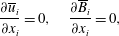 $$\begin{eqnarray}\frac{\unicode[STIX]{x2202}\overline{u}_{i}}{\unicode[STIX]{x2202}x_{i}}=0,\quad \frac{\unicode[STIX]{x2202}\overline{B}_{i}}{\unicode[STIX]{x2202}x_{i}}=0,\end{eqnarray}$$
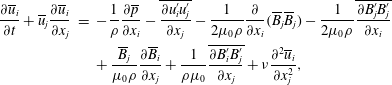 $$\begin{eqnarray}\displaystyle \frac{\unicode[STIX]{x2202}\overline{u}_{i}}{\unicode[STIX]{x2202}t}+\overline{u}_{j}\frac{\unicode[STIX]{x2202}\overline{u}_{i}}{\unicode[STIX]{x2202}x_{j}} & = & \displaystyle -\frac{1}{\unicode[STIX]{x1D70C}}\frac{\unicode[STIX]{x2202}\overline{p}}{\unicode[STIX]{x2202}x_{i}}-\overline{\frac{\unicode[STIX]{x2202}u_{i}^{\prime }u_{j}^{\prime }}{\unicode[STIX]{x2202}x_{j}}}-\frac{1}{2\unicode[STIX]{x1D707}_{0}\unicode[STIX]{x1D70C}}\frac{\unicode[STIX]{x2202}}{\unicode[STIX]{x2202}x_{i}}(\overline{B}_{j}\overline{B}_{j})-\frac{1}{2\unicode[STIX]{x1D707}_{0}\unicode[STIX]{x1D70C}}\overline{\frac{\unicode[STIX]{x2202}B_{j}^{\prime }B_{j}^{\prime }}{\unicode[STIX]{x2202}x_{i}}}\nonumber\\ \displaystyle & & \displaystyle +\,\frac{\overline{B}_{j}}{\unicode[STIX]{x1D707}_{0}\unicode[STIX]{x1D70C}}\frac{\unicode[STIX]{x2202}\overline{B}_{i}}{\unicode[STIX]{x2202}x_{j}}+\frac{1}{\unicode[STIX]{x1D70C}\unicode[STIX]{x1D707}_{0}}\overline{\frac{\unicode[STIX]{x2202}B_{i}^{\prime }B_{j}^{\prime }}{\unicode[STIX]{x2202}x_{j}}}+\unicode[STIX]{x1D708}\frac{\unicode[STIX]{x2202}^{2}\overline{u}_{i}}{\unicode[STIX]{x2202}x_{j}^{2}},\end{eqnarray}$$
 $$\begin{eqnarray}\displaystyle \frac{\unicode[STIX]{x2202}\overline{B}_{i}}{\unicode[STIX]{x2202}t}+\overline{u}_{j}\frac{\unicode[STIX]{x2202}\overline{B}_{i}}{\unicode[STIX]{x2202}x_{j}} & = & \displaystyle \overline{B}_{j}\frac{\unicode[STIX]{x2202}\overline{u}_{i}}{\unicode[STIX]{x2202}x_{j}}+\overline{\frac{\unicode[STIX]{x2202}}{\unicode[STIX]{x2202}x_{j}}\left(u_{i}^{\prime }B_{j}^{\prime }-u_{j}^{\prime }B_{i}^{\prime }\right)}+\unicode[STIX]{x1D702}\frac{\unicode[STIX]{x2202}^{2}\overline{B}_{i}}{\unicode[STIX]{x2202}x_{j}\unicode[STIX]{x2202}x_{j}},\end{eqnarray}$$
where
 $i,j$
vary from 1 to 3, and
 $\unicode[STIX]{x1D702}=1/\unicode[STIX]{x1D707}_{0}\unicode[STIX]{x1D70E}$
is the magnetic diffusivity of the MHD fluid. Einstein summation convention is used. Overbars indicate ensemble averaging. For the case of homogeneous shear flows, the ensemble average is equivalent to the spatial average on the streamwise–spanwise plane.
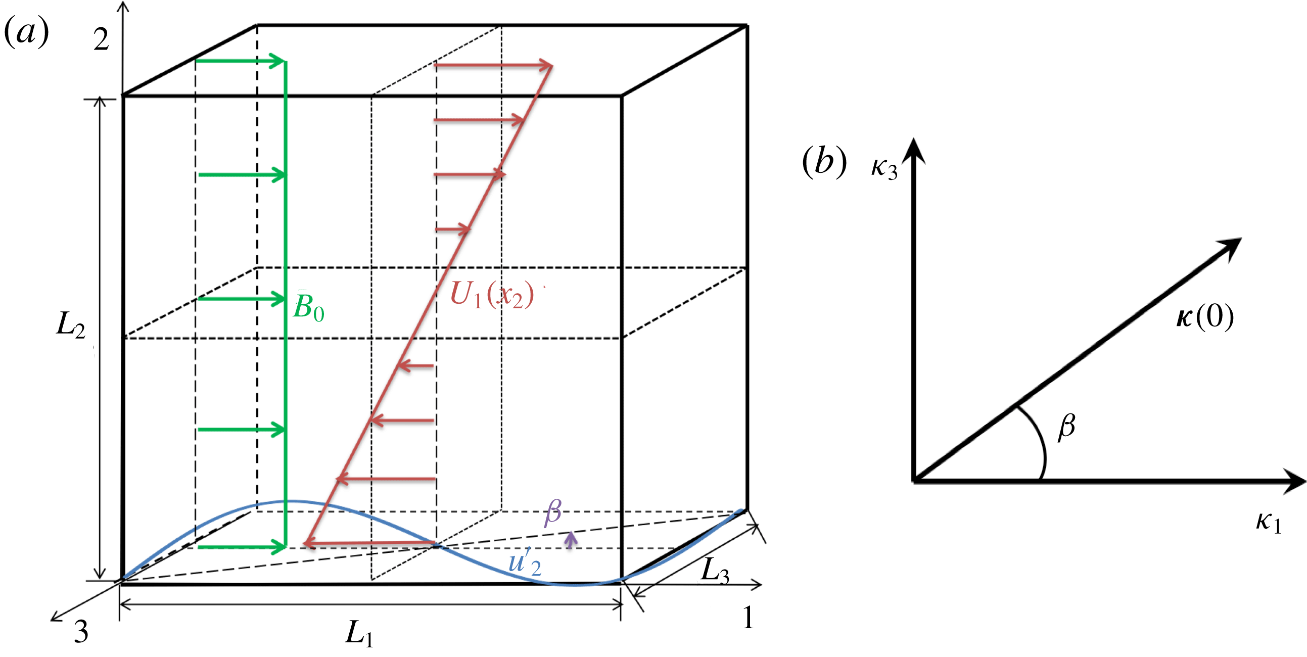
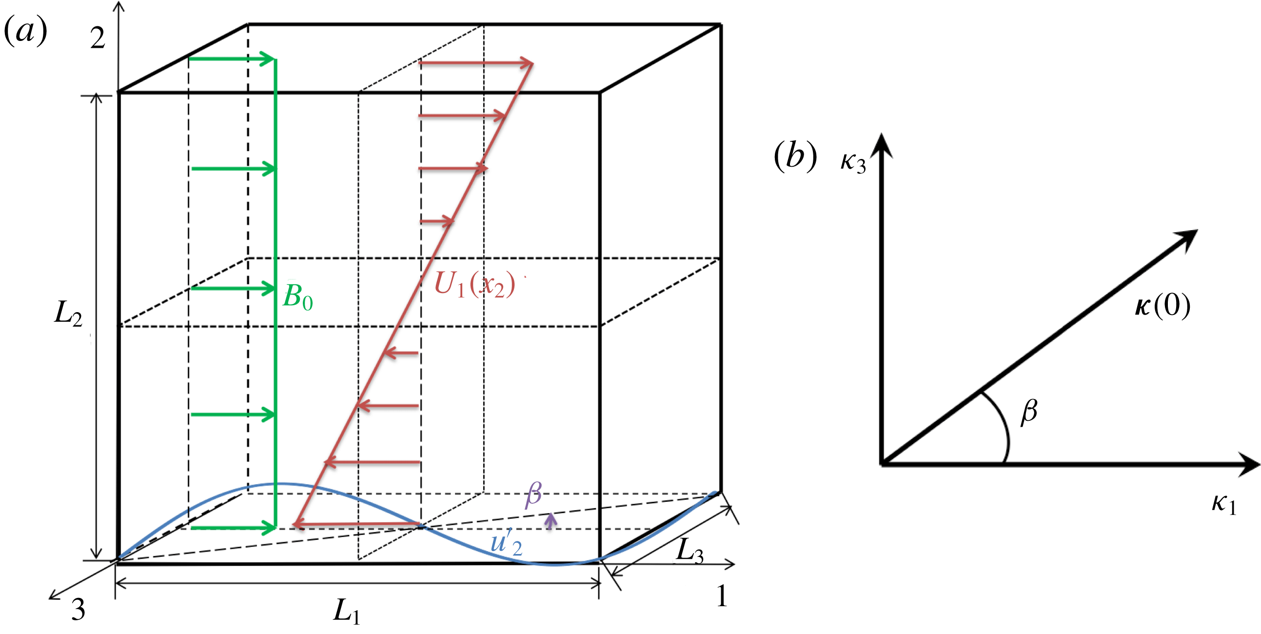
(a) Problem setup. (b) Wavevector orientation with respect to the streamwise direction.
3 Linear analysis
The setup for linear analysis and numerical simulations is shown in figure 1(a). The mean velocity is oriented along the 1 direction and it varies along the 2 direction. The magnetic field is applied in the 1 direction. The colinear alignment of velocity and magnetic fields is seen in plasma propulsion jets such as the variable specific impulse magnetoplasma rocket (VASIMR) engine (Diaz Reference Diaz2000). Other magnetic field orientations will be considered in the future. In subsequent discussions, the 1, 2 and 3 directions will be referred as streamwise, normal and spanwise directions. For this study we consider
 $$\begin{eqnarray}\bar{\boldsymbol{u}}\equiv (U_{1}(x_{2}),0,0),\quad \bar{\boldsymbol{B}}\equiv (B_{0},0,0).\end{eqnarray}$$
Mean density is taken to be uniform. For linear analysis, we consider an ideal MHD fluid. In DNS, the full nonlinear and viscous/resistive effects are included. Under the assumptions of idealized MHD linear analysis, mean pressure is uniform throughout the flow field:
 $$\begin{eqnarray}\frac{\unicode[STIX]{x2202}\overline{p}}{\unicode[STIX]{x2202}x_{i}}=0.\end{eqnarray}$$
The evolution of fluctuating fields is isolated by subtracting the mean field evolution terms from the total field evolution equations upon neglecting nonlinear terms. The resulting equations are (Chagelishvili et al. Reference Chagelishvili, Hristov, Chanishvili and Lominadze1993)
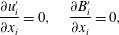 $$\begin{eqnarray}\frac{\unicode[STIX]{x2202}u_{i}^{\prime }}{\unicode[STIX]{x2202}x_{i}}=0,\quad \frac{\unicode[STIX]{x2202}B_{i}^{\prime }}{\unicode[STIX]{x2202}x_{i}}=0,\end{eqnarray}$$
 $$\begin{eqnarray}\displaystyle & \displaystyle \frac{\overline{\text{D}}u_{i}^{\prime }}{\overline{\text{D}}t}\equiv \frac{\unicode[STIX]{x2202}u_{i}^{\prime }}{\unicode[STIX]{x2202}t}+U_{1}(x_{2})\frac{\unicode[STIX]{x2202}u_{i}^{\prime }}{\unicode[STIX]{x2202}x_{1}}=-u_{2}^{\prime }S\unicode[STIX]{x1D6FF}_{i1}-\frac{1}{\unicode[STIX]{x1D70C}}\frac{\unicode[STIX]{x2202}}{\unicode[STIX]{x2202}x_{i}}\left(p^{\prime }+\frac{B_{0}B_{1}^{\prime }}{\unicode[STIX]{x1D707}_{0}}\right)+\frac{B_{0}}{\unicode[STIX]{x1D70C}\unicode[STIX]{x1D707}_{0}}\frac{\unicode[STIX]{x2202}B_{i}^{\prime }}{\unicode[STIX]{x2202}x_{1}} & \displaystyle\end{eqnarray}$$
 $$\begin{eqnarray}\displaystyle & \displaystyle \frac{\overline{\text{D}}B_{i}^{\prime }}{\overline{\text{D}}t}\equiv \frac{\unicode[STIX]{x2202}B_{i}^{\prime }}{\unicode[STIX]{x2202}t}+U_{1}(x_{2})\frac{\unicode[STIX]{x2202}B_{i}^{\prime }}{\unicode[STIX]{x2202}x_{1}}=B_{2}^{\prime }S\unicode[STIX]{x1D6FF}_{i1}+B_{0}\frac{\unicode[STIX]{x2202}u_{i}^{\prime }}{\unicode[STIX]{x2202}x_{1}}, & \displaystyle\end{eqnarray}$$
where the uniform flow shear is given by
 $$\begin{eqnarray}S\equiv \frac{\text{d}U_{1}}{\text{d}x_{2}}.\end{eqnarray}$$
A coordinate frame (
 $\boldsymbol{X}$
) that convects and deforms with the mean flow is utilized to examine the flow evolution (Rogallo Reference Rogallo1981):
 $$\begin{eqnarray}X_{1}=x_{1}-\int _{0}^{t}U_{1}(x_{2})\,\text{d}\unicode[STIX]{x1D709},\quad X_{2}=x_{2},\quad X_{3}=x_{3},\quad t=t.\end{eqnarray}$$
Equations in the convective coordinate frame (
 $\boldsymbol{X}$
) then become
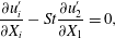 $$\begin{eqnarray}\displaystyle & \displaystyle \frac{\unicode[STIX]{x2202}u_{i}^{\prime }}{\unicode[STIX]{x2202}X_{i}}-St\frac{\unicode[STIX]{x2202}u_{2}^{\prime }}{\unicode[STIX]{x2202}X_{1}}=0, & \displaystyle\end{eqnarray}$$
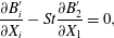 $$\begin{eqnarray}\displaystyle & \displaystyle \frac{\unicode[STIX]{x2202}B_{i}^{\prime }}{\unicode[STIX]{x2202}X_{i}}-St\frac{\unicode[STIX]{x2202}B_{2}^{\prime }}{\unicode[STIX]{x2202}X_{1}}=0, & \displaystyle\end{eqnarray}$$
 $$\begin{eqnarray}\displaystyle & \displaystyle \frac{\unicode[STIX]{x2202}u_{i}^{\prime }}{\unicode[STIX]{x2202}t}=-u_{2}^{\prime }S\unicode[STIX]{x1D6FF}_{i1}-\frac{1}{\unicode[STIX]{x1D70C}}\frac{\unicode[STIX]{x2202}p^{\prime }}{\unicode[STIX]{x2202}X_{i}}-\frac{B_{0}}{\unicode[STIX]{x1D70C}\unicode[STIX]{x1D707}_{0}}\frac{\unicode[STIX]{x2202}B_{1}^{\prime }}{\unicode[STIX]{x2202}X_{i}}+\frac{St}{\unicode[STIX]{x1D70C}}\frac{\unicode[STIX]{x2202}p^{\prime }}{\unicode[STIX]{x2202}X_{1}}\unicode[STIX]{x1D6FF}_{i2}+\frac{StB_{0}}{\unicode[STIX]{x1D70C}\unicode[STIX]{x1D707}_{0}}\frac{\unicode[STIX]{x2202}B_{1}^{\prime }}{\unicode[STIX]{x2202}X_{1}}\unicode[STIX]{x1D6FF}_{i2}+\frac{B_{0}}{\unicode[STIX]{x1D70C}\unicode[STIX]{x1D707}_{0}}\frac{\unicode[STIX]{x2202}B_{i}^{\prime }}{\unicode[STIX]{x2202}X_{1}}, & \displaystyle\end{eqnarray}$$
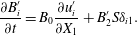 $$\begin{eqnarray}\displaystyle & \displaystyle \frac{\unicode[STIX]{x2202}B_{i}^{\prime }}{\unicode[STIX]{x2202}t}=B_{0}\frac{\unicode[STIX]{x2202}u_{i}^{\prime }}{\unicode[STIX]{x2202}X_{1}}+B_{2}^{\prime }S\unicode[STIX]{x1D6FF}_{i1}. & \displaystyle\end{eqnarray}$$
Following RDT methodology (Taylor & Batchelor Reference Taylor and Batchelor1949; Batchelor & Proudman Reference Batchelor and Proudman1954; Cambon, Coleman & Mansour Reference Cambon, Coleman and Mansour1993; Pope Reference Pope2001), we now consider perturbations that are periodic in all
 $X_{i}$
directions:
 $$\begin{eqnarray}q^{\prime }(\boldsymbol{X},t)=\hat{q}(t)\text{e}^{\text{i}\unicode[STIX]{x1D73F}(\mathbf{0})\boldsymbol{\cdot }\boldsymbol{X}}=\hat{q}(t)\text{e}^{\text{i}\unicode[STIX]{x1D73F}(\boldsymbol{t})\boldsymbol{\cdot }\boldsymbol{x}}.\end{eqnarray}$$
Owing to the coordinate transformation, the wavenumbers evolve as (Pope Reference Pope2001)
 $$\begin{eqnarray}\frac{\text{d}\unicode[STIX]{x1D705}_{i}}{\text{d}t}=-\unicode[STIX]{x1D705}_{j}\frac{\unicode[STIX]{x2202}U_{j}}{\unicode[STIX]{x2202}x_{i}}.\end{eqnarray}$$
For the mean velocity profile (
 $U_{1}(x_{2})$
) considered in this study, the above equation reduces to
 $$\begin{eqnarray}\frac{\text{d}\unicode[STIX]{x1D705}_{1}}{\text{d}t}=0,\quad \frac{\text{d}\unicode[STIX]{x1D705}_{2}}{\text{d}t}=-\unicode[STIX]{x1D705}_{1}S,\quad \frac{\text{d}\unicode[STIX]{x1D705}_{3}}{\text{d}t}=0,\end{eqnarray}$$
leading to
 $$\begin{eqnarray}\unicode[STIX]{x1D705}_{1}(t)=\unicode[STIX]{x1D705}_{1}(0),\quad \unicode[STIX]{x1D705}_{2}(t)=\unicode[STIX]{x1D705}_{2}(0)-St\unicode[STIX]{x1D705}_{1}(0),\quad \unicode[STIX]{x1D705}_{3}(t)=\unicode[STIX]{x1D705}_{3}(0).\end{eqnarray}$$
The implication is that the wavevector magnitude and direction in the streamwise–spanwise plane remain constant, and the wavenumber in the normal direction grows linearly. The perturbation amplitudes evolve as (using (3.14d–f ))
 $$\begin{eqnarray}\displaystyle & \displaystyle \frac{\text{d}\hat{u} _{i}}{\text{d}t}=-\hat{u} _{2}S\unicode[STIX]{x1D6FF}_{i1}-\text{i}\unicode[STIX]{x1D705}_{i}\left(\frac{\hat{p}}{\unicode[STIX]{x1D70C}}+\frac{B_{0}}{\unicode[STIX]{x1D70C}\unicode[STIX]{x1D707}_{0}}\hat{B}_{1}\right)+\frac{B_{0}}{\unicode[STIX]{x1D70C}\unicode[STIX]{x1D707}_{0}}\text{i}\unicode[STIX]{x1D705}_{1}\hat{B}_{i}, & \displaystyle\end{eqnarray}$$
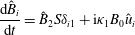 $$\begin{eqnarray}\displaystyle & \displaystyle \frac{\text{d}\hat{B}_{i}}{\text{d}t}=\hat{B}_{2}S\unicode[STIX]{x1D6FF}_{i1}+\text{i}\unicode[STIX]{x1D705}_{1}B_{0}\hat{u} _{i} & \displaystyle\end{eqnarray}$$
subject to the divergence-free constraints
 $$\begin{eqnarray}\text{i}\unicode[STIX]{x1D705}_{i}\hat{u} _{i}=0,\quad \text{i}\unicode[STIX]{x1D705}_{i}\hat{B}_{i}=0.\end{eqnarray}$$
It is evident from the above equations that the stability characteristics of the linear system are contingent on the initial wavenumber of the perturbations. The equations demonstrate that
 $\unicode[STIX]{x1D705}_{2}$
plays a critical role in the perturbation evolution as it is the only wavenumber component that changes with time. We consider two distinct classes of initial conditions:
 $\unicode[STIX]{x1D705}_{2}\neq 0$
and
 $\unicode[STIX]{x1D705}_{2}=0$
.
Initial perturbations with
 $\unicode[STIX]{x1D705}_{2}(0)\neq 0$
. In the early stages, the initial value of
 $\unicode[STIX]{x1D705}_{2}$
plays a critical role in determining the evolution of the perturbations. This transient stage can have interesting implications on perturbation growth. Chagelishvili et al. (Reference Chagelishvili, Hristov, Chanishvili and Lominadze1993) have investigated the early-time energy interactions for two-dimensional perturbations on the streamwise–normal (
 $\unicode[STIX]{x1D705}_{1}$
–
 $\unicode[STIX]{x1D705}_{2}$
) plane. Further analytical examination of this parameter regime will performed in future works.
Initial perturbations with
 $\unicode[STIX]{x1D705}_{2}(0)=0$
. In this study, we focus on perturbations that are initially located on the
 $\unicode[STIX]{x1D705}_{1}$
–
 $\unicode[STIX]{x1D705}_{3}$
plane for several reasons. First and foremost, these perturbations provide crucial insight into the long-term stability characteristics of general shear flow instabilities subject to streamwise magnetic field. Second, owing to the nature of
 $\unicode[STIX]{x1D705}_{2}$
growth, the asymptotic stability of the linear equations can be completely captured by this initial condition. Finally, this system is amenable to rigorous mathematical analysis, which leads to profound insight into the stabilizing influence of magnetic field. We express these initial wavevectors in terms of their magnitude
 $\unicode[STIX]{x1D705}_{0}$
and orientation
 $\unicode[STIX]{x1D6FD}$
with respect to the streamwise direction (see figure 1
b). The wavenumber equation (3.14d–f
) can be written as
 $$\begin{eqnarray}\unicode[STIX]{x1D705}_{1}(t)=\unicode[STIX]{x1D705}_{0}\cos \unicode[STIX]{x1D6FD},\quad \unicode[STIX]{x1D705}_{2}(t)=-\unicode[STIX]{x1D705}_{0}St\cos \unicode[STIX]{x1D6FD},\quad \unicode[STIX]{x1D705}_{3}(t)=\unicode[STIX]{x1D705}_{0}\sin \unicode[STIX]{x1D6FD}.\end{eqnarray}$$
The Poisson equation for total pressure amplitude (
 $\hat{p}+B_{0}\hat{B}_{1}/\unicode[STIX]{x1D707}_{0}$
) can be obtained using (3.14b
), (3.15) and (3.17):
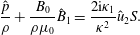 $$\begin{eqnarray}\frac{\hat{p}}{\unicode[STIX]{x1D70C}}+\frac{B_{0}}{\unicode[STIX]{x1D70C}\unicode[STIX]{x1D707}_{0}}\hat{B}_{1}=\frac{2\text{i}\unicode[STIX]{x1D705}_{1}}{\unicode[STIX]{x1D705}^{2}}\hat{u} _{2}S.\end{eqnarray}$$
Equation (3.15) then becomes
 $$\begin{eqnarray}\frac{\text{d}\hat{u} _{i}}{\text{d}t}=\hat{u} _{2}S\left(-\unicode[STIX]{x1D6FF}_{i1}+\frac{2\unicode[STIX]{x1D705}_{1}\unicode[STIX]{x1D705}_{i}}{\unicode[STIX]{x1D705}^{2}}\right)+\text{i}\frac{B_{0}}{\unicode[STIX]{x1D70C}\unicode[STIX]{x1D707}_{0}}\unicode[STIX]{x1D705}_{1}\hat{B}_{i}.\end{eqnarray}$$
The perturbation equations (3.16) and (3.20) are non-dimensionalized using the Alfvén wave speed (
 $V_{A}$
), mean flow shear, initial wavenumber and imposed magnetic field:
 $$\begin{eqnarray}u_{i}^{\ast }=u_{i}/V_{A},\quad V_{A}=\frac{B_{0}}{\sqrt{\unicode[STIX]{x1D70C}\unicode[STIX]{x1D707}_{0}}},\quad \unicode[STIX]{x1D70F}=St,\quad \unicode[STIX]{x1D705}_{i}^{\ast }=\unicode[STIX]{x1D705}_{i}/\unicode[STIX]{x1D705}_{0},\quad B_{i}^{\ast }=B_{i}/B_{0}.\end{eqnarray}$$
Finally, the governing dimensionless equations are
 $$\begin{eqnarray}\displaystyle & \displaystyle \frac{\text{d}\hat{u} _{i}^{\ast }}{\text{d}\unicode[STIX]{x1D70F}}=\hat{u} _{2}^{\ast }\left(-\unicode[STIX]{x1D6FF}_{i1}+\frac{2\cos (\unicode[STIX]{x1D6FD})\unicode[STIX]{x1D705}_{i}^{\ast }}{1+\cos ^{2}(\unicode[STIX]{x1D6FD})\unicode[STIX]{x1D70F}^{2}}\right)+\text{i}R_{A}\cos (\unicode[STIX]{x1D6FD})\hat{B}_{i}^{\ast }, & \displaystyle\end{eqnarray}$$
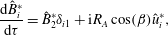 $$\begin{eqnarray}\displaystyle & \displaystyle \frac{\text{d}\hat{B}_{i}^{\ast }}{\text{d}\unicode[STIX]{x1D70F}}=\hat{B}_{2}^{\ast }\unicode[STIX]{x1D6FF}_{i1}+\text{i}R_{A}\cos (\unicode[STIX]{x1D6FD})\hat{u} _{i}^{\ast }, & \displaystyle\end{eqnarray}$$
where
 $$\begin{eqnarray}R_{A}\equiv \frac{\unicode[STIX]{x1D705}_{0}V_{A}}{S}=\frac{\text{shear timescale}}{\text{magnetic timescale}}.\end{eqnarray}$$
From the above equations, it can be seen that the flow behaviour can be completely characterized in terms of the parameters
 $R_{A}$
and
 $\unicode[STIX]{x1D6FD}$
. The role of
 $R_{A}$
has been recognized to some extent in the other studies (Chagelishvili et al.
Reference Chagelishvili, Hristov, Chanishvili and Lominadze1993). The influence of
 $\unicode[STIX]{x1D6FD}$
is examined in detail for the first time in this study. Equations (3.22) and (3.23) clearly indicate that the velocity and magnetic field perturbations are coupled via the last terms on their right-hand sides. Here
 $R_{A}\cos (\unicode[STIX]{x1D6FD})$
is the coupling parameter in the problem. Therefore, for a given value of
 $R_{A}$
, streamwise perturbations experience the highest degree of coupling. The coupling becomes weaker with increasing
 $\unicode[STIX]{x1D6FD}$
. For spanwise orientations, velocity and magnetic field perturbations are decoupled.
We now investigate the evolution of the magnitudes of velocity and magnetic perturbation amplitudes. For ease of notation, we denote the dimensionless variables
 $q^{\ast }$
as
 $q$
. To obtain the evolution equation for perturbation kinetic energy, we multiply equation (3.22) by
 $\bar{\hat{u} }_{i}$
, the complex conjugate of
 $\hat{u} _{i}$
,
 $$\begin{eqnarray}\bar{\hat{u} }_{i}\frac{\text{d}\hat{u} _{i}}{\text{d}\unicode[STIX]{x1D70F}}=\bar{\hat{u} }_{i}\hat{u} _{2}\left(-\unicode[STIX]{x1D6FF}_{i1}+\frac{2\cos (\unicode[STIX]{x1D6FD})\unicode[STIX]{x1D705}_{i}}{1+\cos ^{2}(\unicode[STIX]{x1D6FD})\unicode[STIX]{x1D70F}^{2}}\right)+\text{i}R_{A}\cos (\unicode[STIX]{x1D6FD})\hat{B}_{i}\bar{\hat{u} }_{i}.\end{eqnarray}$$
Utilizing the complex conjugate of the continuity equation (3.17a ), the above kinetic energy equation (3.25) reduces to
 $$\begin{eqnarray}\bar{\hat{u} }_{i}\frac{\text{d}\hat{u} _{i}}{\text{d}\unicode[STIX]{x1D70F}}=-\bar{\hat{u} }_{i}\hat{u} _{2}\unicode[STIX]{x1D6FF}_{i1}+\text{i}R_{A}\cos (\unicode[STIX]{x1D6FD})\hat{B}_{i}\bar{\hat{u} }_{i}.\end{eqnarray}$$
Similarly, equation (3.23) is multiplied by
 $\bar{\hat{B}}_{i}$
(the complex conjugate of
 $\hat{B}_{i}$
) to obtain the magnetic energy equation:
 $$\begin{eqnarray}\bar{\hat{B}}_{i}\frac{\text{d}\hat{B}_{i}}{\text{d}\unicode[STIX]{x1D70F}}=\bar{\hat{B}}_{i}\hat{B}_{2}\unicode[STIX]{x1D6FF}_{i1}+\text{i}R_{A}\cos (\unicode[STIX]{x1D6FD})\bar{\hat{B}}_{i}\hat{u} _{i}.\end{eqnarray}$$
Summing (3.26) and (3.27) with their complex conjugate counterparts yields
 $$\begin{eqnarray}\displaystyle & \displaystyle \frac{1}{2}\frac{\text{d}\hat{u} _{i}\bar{\hat{u} }_{i}}{\text{d}\unicode[STIX]{x1D70F}}=-\text{Re}(\bar{\hat{u} }_{i}\hat{u} _{2})\unicode[STIX]{x1D6FF}_{i1}-R_{A}\cos (\unicode[STIX]{x1D6FD})\text{Im}(\hat{B}_{i}\bar{\hat{u} }_{i}), & \displaystyle\end{eqnarray}$$
 $$\begin{eqnarray}\displaystyle & \displaystyle \frac{1}{2}\frac{\text{d}\hat{B}_{i}\bar{\hat{B}}_{i}}{\text{d}\unicode[STIX]{x1D70F}}=\text{Re}(\hat{B}_{2}\bar{\hat{B}}_{i})\unicode[STIX]{x1D6FF}_{i1}+R_{A}\cos (\unicode[STIX]{x1D6FD})\text{Im}(\hat{B}_{i}\bar{\hat{u} }_{i}), & \displaystyle\end{eqnarray}$$
where
 $\text{Re}(q),\text{Im}(q)$
indicate the real and imaginary parts of a complex quantity
 $q$
. The first term on the right-hand side of (3.28) represents production, the process in which perturbation kinetic energy is transferred from the mean flow. Similarly, the first term on the right-hand side of (3.29) represents magnetic stretching, the process in which perturbation magnetic energy is produced by the stretching action of the mean flow. Production and magnetic stretching occur at shear (
 $S$
) timescale. It can be seen that the last terms on the right-hand side of (3.28), (3.29) are identical, but with opposite signs. This implies that they result in a harmonic exchange between magnetic and kinetic energies. The harmonic exchange process takes place at the timescale,
 $V_{A}\unicode[STIX]{x1D705}_{0}\cos (\unicode[STIX]{x1D6FD})$
. Therefore,
 $R_{A}\cos \unicode[STIX]{x1D6FD}$
determines the relative timescales of production and exchange processes.
We next investigate the energy transfer among individual components of kinetic and magnetic energies. We utilize the following notation for various energies for the sake of simplicity:
 $$\begin{eqnarray}k\equiv \hat{u} _{i}\bar{\hat{u} }_{i},\quad k_{1}\equiv \hat{u} _{1}\bar{\hat{u} }_{1},\quad k_{2}\equiv \hat{u} _{2}\bar{\hat{u} }_{2},\quad k_{3}\equiv \hat{u} _{3}\bar{\hat{u} }_{3},\end{eqnarray}$$
 $$\begin{eqnarray}b\equiv \hat{B}_{i}\bar{\hat{B}}_{i},\quad b_{1}\equiv \hat{B}_{1}\bar{\hat{B}}_{1},\quad b_{2}\equiv \hat{B}_{2}\bar{\hat{B}}_{2},\quad b_{3}\equiv \hat{B}_{3}\bar{\hat{B}}_{3}.\end{eqnarray}$$
The governing equations for the energies in velocity components are
 $$\begin{eqnarray}\displaystyle & \displaystyle \frac{\text{d}k_{1}}{\text{d}\unicode[STIX]{x1D70F}}\equiv \frac{\text{d}(\hat{u} _{1}\bar{\hat{u} }_{1}\!)}{\text{d}\unicode[STIX]{x1D70F}}=2\text{Re}(\hat{u} _{2}\bar{\hat{u} }_{1}\!)\frac{2\cos ^{2}(\unicode[STIX]{x1D6FD})}{1+\cos ^{2}(\unicode[STIX]{x1D6FD})\unicode[STIX]{x1D70F}^{2}}-\!2\text{Re}(\hat{u} _{2}\bar{\hat{u} }_{1})\!-2R_{A}\cos (\unicode[STIX]{x1D6FD})\text{Im}(\hat{B}_{1}\bar{\hat{u} }_{1}),\qquad & \displaystyle\end{eqnarray}$$
 $$\begin{eqnarray}\displaystyle & \displaystyle \frac{\text{d}k_{2}}{\text{d}\unicode[STIX]{x1D70F}}\equiv \frac{\text{d}(\hat{u} _{2}\bar{\hat{u} }_{2})}{\text{d}\unicode[STIX]{x1D70F}}=-2\text{Re}(\hat{u} _{2}\bar{\hat{u} }_{2})\frac{2\cos ^{2}(\unicode[STIX]{x1D6FD})\unicode[STIX]{x1D70F}}{1+\cos ^{2}(\unicode[STIX]{x1D6FD})\unicode[STIX]{x1D70F}^{2}}-2R_{A}\cos (\unicode[STIX]{x1D6FD})\text{Im}(\hat{B}_{2}\bar{\hat{u} }_{2}), & \displaystyle\end{eqnarray}$$
 $$\begin{eqnarray}\displaystyle & \displaystyle \frac{\text{d}k_{3}}{\text{d}\unicode[STIX]{x1D70F}}\equiv \frac{\text{d}(\hat{u} _{3}\bar{\hat{u} }_{3})}{\text{d}\unicode[STIX]{x1D70F}}=2\text{Re}(\hat{u} _{2}\bar{\hat{u} }_{3})\frac{2\cos (\unicode[STIX]{x1D6FD})\sin (\unicode[STIX]{x1D6FD})}{1+\cos ^{2}(\unicode[STIX]{x1D6FD})\unicode[STIX]{x1D70F}^{2}}-2R_{A}\cos (\unicode[STIX]{x1D6FD})\text{Im}(\hat{B}_{3}\bar{\hat{u} }_{3}). & \displaystyle\end{eqnarray}$$
 $\hat{u} _{i}$
in (3.22) to impose divergence-free constraint. Total pressure redistributes the energy amongst different velocity components to satisfy continuity. Production and pressure redistribution in (3.31a
) have opposing effects as can be seen from the coefficients of
 $\hat{u} _{2}\bar{\hat{u} }_{1}$
. The coefficient of production is always negative
 $(-1)$
, whereas the coefficient of pressure redistribution is always positive. The nature of the term
 $\bar{\hat{u} }_{1}\hat{u} _{2}$
can be deduced using the continuity equation:
 $$\begin{eqnarray}\hat{u} _{1}\unicode[STIX]{x1D705}_{1}+\hat{u} _{2}\unicode[STIX]{x1D705}_{2}+\hat{u} _{3}\unicode[STIX]{x1D705}_{3}=0.\end{eqnarray}$$
Substituting for the values of
 $\unicode[STIX]{x1D705}_{i}$
using (3.18),
 $$\begin{eqnarray}\hat{u} _{1}\cos \unicode[STIX]{x1D6FD}-\unicode[STIX]{x1D70F}\hat{u} _{2}\cos \unicode[STIX]{x1D6FD}+\hat{u} _{3}\sin \unicode[STIX]{x1D6FD}=0.\end{eqnarray}$$
Multiplying the above equation by the complex conjugate of
 $\hat{u} _{1}$
,
 $$\begin{eqnarray}\cos \unicode[STIX]{x1D6FD}|\hat{u} _{1}|^{2}+\bar{\hat{u} }_{1}\hat{u} _{3}\sin \unicode[STIX]{x1D6FD}=\unicode[STIX]{x1D70F}\bar{\hat{u} }_{1}\hat{u} _{2}\cos \unicode[STIX]{x1D6FD}.\end{eqnarray}$$
Therefore, the term
 $\bar{\hat{u} }_{1}\hat{u} _{2}$
can be written as
 $$\begin{eqnarray}\bar{\hat{u} }_{1}\hat{u} _{2}=\frac{1}{\unicode[STIX]{x1D70F}}(|\hat{u} _{1}|^{2}+\bar{\hat{u} }_{1}\hat{u} _{3}\tan \unicode[STIX]{x1D6FD}).\end{eqnarray}$$
For
 $\unicode[STIX]{x1D6FD}=0^{\circ }$
, the continuity equation stipulates
 $\bar{\hat{u} }_{1}\hat{u} _{2}$
to be always positive. For other orientations,
 $\bar{\hat{u} }_{1}\hat{u} _{2}$
could be positive or negative depending upon the initial conditions. However, the value of
 $\bar{\hat{u} }_{1}\hat{u} _{2}$
for all orientations decreases with time as
 $\unicode[STIX]{x1D70F}^{-1}$
.
The evolution equations for energies in the magnetic field components are given by
 $$\begin{eqnarray}\displaystyle & \displaystyle \frac{\text{d}b_{1}}{\text{d}\unicode[STIX]{x1D70F}}\equiv \frac{\text{d}(\hat{B}_{1}\bar{\hat{B}}_{1})}{\text{d}\unicode[STIX]{x1D70F}}=2\text{Re}(\hat{B}_{2}\bar{\hat{B}}_{1})+2R_{A}\cos (\unicode[STIX]{x1D6FD})\text{Im}(\hat{B}_{1}\bar{\hat{u} }_{1}), & \displaystyle\end{eqnarray}$$
 $$\begin{eqnarray}\displaystyle & \displaystyle \frac{\text{d}b_{2}}{\text{d}\unicode[STIX]{x1D70F}}\equiv \frac{\text{d}(\hat{B}_{2}\bar{\hat{B}}_{2})}{\text{d}\unicode[STIX]{x1D70F}}=2R_{A}\cos (\unicode[STIX]{x1D6FD})\text{Im}(\hat{B}_{2}\bar{\hat{u} }_{2}), & \displaystyle\end{eqnarray}$$
 $$\begin{eqnarray}\displaystyle & \displaystyle \frac{\text{d}b_{3}}{\text{d}\unicode[STIX]{x1D70F}}\equiv \frac{\text{d}(\hat{B}_{3}\bar{\hat{B}}_{3})}{\text{d}\unicode[STIX]{x1D70F}}=2R_{A}\cos (\unicode[STIX]{x1D6FD})\text{Im}(\hat{B}_{3}\bar{\hat{u} }_{3}). & \displaystyle\end{eqnarray}$$
 $\hat{u} _{2}\bar{\hat{u} }_{1}$
can be drawn regarding the magnetic stretching production term
 $\hat{B}_{2}\bar{\hat{B}}_{1}$
:
 $$\begin{eqnarray}\bar{\hat{B}}_{1}\hat{B}_{2}=\frac{1}{\unicode[STIX]{x1D70F}}(|\hat{B}_{1}|^{2}+\bar{\hat{B}}_{1}\hat{B}_{3}\tan \unicode[STIX]{x1D6FD}).\end{eqnarray}$$
Overall, the energy interactions involve four important processes: production, magnetic stretching, pressure redistribution and harmonic kinetic–magnetic exchange. It can be observed that production and magnetic stretching depend on the behaviour of normal components of velocity and magnetic fields,
 $u_{2}^{\prime },B_{2}^{\prime }$
. Therefore, it is crucial to examine the evolution of
 $u_{2}^{\prime },B_{2}^{\prime }$
at different
 $R_{A},\unicode[STIX]{x1D6FD}$
.
We examine the evolution of spanwise perturbations (
 $\unicode[STIX]{x1D6FD}=90^{\circ }$
) first, followed by an investigation of other orientations (
 $\unicode[STIX]{x1D6FD}\in [\!0^{\circ },90^{\circ }\!)$
).
3.1 Regimes of evolution
3.1.1 Spanwise perturbations,
$\unicode[STIX]{x1D6FD}=90^{\circ }$

As seen in previous sections, this represents a special limit because the velocity and magnetic fields are decoupled. The wavevectors remain at their initial state:
 $$\begin{eqnarray}\unicode[STIX]{x1D705}_{1}(t)=0,\quad \unicode[STIX]{x1D705}_{2}(t)=0,\quad \unicode[STIX]{x1D705}_{3}(t)=\unicode[STIX]{x1D705}_{3}(0).\end{eqnarray}$$
The total pressure Poisson equation becomes
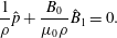 $$\begin{eqnarray}\frac{1}{\unicode[STIX]{x1D70C}}\hat{p}+\frac{B_{0}}{\unicode[STIX]{x1D707}_{0}\unicode[STIX]{x1D70C}}\hat{B}_{1}=0.\end{eqnarray}$$
The individual velocity components evolve as
 $$\begin{eqnarray}\frac{\text{d}\hat{u} _{1}}{\text{d}\unicode[STIX]{x1D70F}}=-\hat{u} _{2},\quad \frac{\text{d}\hat{u} _{2}}{\text{d}\unicode[STIX]{x1D70F}}=0,\quad \frac{\text{d}\hat{u} _{3}}{\text{d}\unicode[STIX]{x1D70F}}=0.\end{eqnarray}$$
The velocity equations are unaffected by pressure similar to spanwise perturbations in hydrodynamic homogeneous shear flow (Kumar et al. Reference Kumar, Bertsch and Girimaji2014). This is called pressure-released behaviour (Simone, Coleman & Cambon Reference Simone, Coleman and Cambon1997). Integrating the above equations,
 $$\begin{eqnarray}\hat{u} _{1}(\unicode[STIX]{x1D70F})=-\hat{u} _{2}(0)\unicode[STIX]{x1D70F}+\hat{u} _{1}(0),\quad \hat{u} _{2}(\unicode[STIX]{x1D70F})=\hat{u} _{2}(0),\quad \hat{u} _{3}(\unicode[STIX]{x1D70F})=\hat{u} _{3}(0).\end{eqnarray}$$
If
 $\hat{u} _{1},\hat{u} _{3}$
are zero initially, the kinetic energy (
 $k$
) in the flow will evolve with respect to the initial kinetic energy (
 $k_{0}$
) as (Simone et al.
Reference Simone, Coleman and Cambon1997)
 $$\begin{eqnarray}\frac{k}{k_{0}}=1+\unicode[STIX]{x1D70F}^{2}.\end{eqnarray}$$
The individual magnetic components evolve as
 $$\begin{eqnarray}\frac{\text{d}\hat{B}_{1}}{\text{d}\unicode[STIX]{x1D70F}}=\hat{B}_{2},\quad \frac{\text{d}\hat{B}_{2}}{\text{d}\unicode[STIX]{x1D70F}}=0,\quad \frac{\text{d}\hat{B}_{3}}{\text{d}\unicode[STIX]{x1D70F}}=0.\end{eqnarray}$$
This implies
 $$\begin{eqnarray}\hat{B}_{1}(\unicode[STIX]{x1D70F})=\hat{B}_{2}(0)\unicode[STIX]{x1D70F}+\hat{B}_{1}(0),\quad \hat{B}_{2}(\unicode[STIX]{x1D70F})=\hat{B}_{2}(0),\quad \hat{B}_{3}(\unicode[STIX]{x1D70F})=\hat{B}_{3}(0).\end{eqnarray}$$
Magnetic perturbations remain unchanged when the initial magnetic energy is zero.
3.1.2 Perturbation orientations with
$\unicode[STIX]{x1D6FD}\in [0^{\circ },90^{\circ })$

Recall that the evolution of kinetic and magnetic energies critically depends on the behaviour of
 $u_{2}^{\prime }$
and
 $B_{2}^{\prime }$
. To eliminate the explicit dependence of
 $\unicode[STIX]{x1D6FD}$
on
 $\hat{u} _{2},\hat{B}_{2}$
, we define a new timescale (
 $\unicode[STIX]{x1D70F}^{\ast }$
), similar to the transformation performed by Dimitrov et al. (Reference Dimitrov, Maneva, Hristov and Mishonov2011):
 $$\begin{eqnarray}\unicode[STIX]{x1D70F}^{\ast }=\unicode[STIX]{x1D70F}\cos \unicode[STIX]{x1D6FD}.\end{eqnarray}$$
The resultant equations are given by
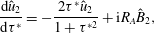 $$\begin{eqnarray}\displaystyle & \displaystyle \frac{\text{d}\hat{u} _{2}}{\text{d}\unicode[STIX]{x1D70F}^{\ast }}=-\frac{2\unicode[STIX]{x1D70F}^{\ast }\hat{u} _{2}}{1+\unicode[STIX]{x1D70F}^{\ast 2}}+\text{i}R_{A}\hat{B}_{2}, & \displaystyle\end{eqnarray}$$
 $$\begin{eqnarray}\displaystyle & \displaystyle \frac{\text{d}\hat{B}_{2}}{\text{d}\unicode[STIX]{x1D70F}^{\ast }}=\text{i}R_{A}\hat{u} _{2}. & \displaystyle\end{eqnarray}$$
This is a coupled system of homogeneous linear ordinary differential equations with
 $R_{A}$
as the coupling parameter. To isolate the evolution of each field, a second derivative with respect to
 $\unicode[STIX]{x1D70F}^{\ast }$
is calculated. The resulting equations are
 $$\begin{eqnarray}\displaystyle & \displaystyle \frac{\text{d}^{2}\hat{u} _{2}}{\text{d}\unicode[STIX]{x1D70F}^{\ast 2}}=-\frac{2\unicode[STIX]{x1D70F}^{\ast }}{1+\unicode[STIX]{x1D70F}^{\ast 2}}\frac{\text{d}\hat{u} _{2}}{\text{d}\unicode[STIX]{x1D70F}^{\ast }}-2\hat{u} _{2}\frac{1-\unicode[STIX]{x1D70F}^{\ast 2}}{(1+\unicode[STIX]{x1D70F}^{\ast 2})^{2}}+\text{i}R_{A}\frac{\text{d}\hat{B}_{2}}{\text{d}\unicode[STIX]{x1D70F}^{\ast }}, & \displaystyle\end{eqnarray}$$
 $$\begin{eqnarray}\displaystyle & \displaystyle \frac{\text{d}^{2}\hat{B}_{2}}{\text{d}\unicode[STIX]{x1D70F}^{\ast 2}}=\text{i}R_{A}\frac{\text{d}\hat{u} _{2}}{\text{d}\unicode[STIX]{x1D70F}^{\ast }}. & \displaystyle\end{eqnarray}$$
 $\hat{u} _{2}$
and
 $\hat{B}_{2}$
are given by
 $$\begin{eqnarray}\displaystyle & \displaystyle \frac{\text{d}^{2}\hat{u} _{2}}{\text{d}\unicode[STIX]{x1D70F}^{\ast 2}}+\frac{2\unicode[STIX]{x1D70F}^{\ast }}{1+\unicode[STIX]{x1D70F}^{\ast 2}}\frac{\text{d}\hat{u} _{2}}{\text{d}\unicode[STIX]{x1D70F}^{\ast }}+2\hat{u} _{2}\frac{1-\unicode[STIX]{x1D70F}^{\ast 2}}{(1+\unicode[STIX]{x1D70F}^{\ast 2})^{2}}+R_{A}^{2}\hat{u} _{2}=0, & \displaystyle\end{eqnarray}$$
 $$\begin{eqnarray}\displaystyle & \displaystyle \frac{\text{d}^{2}\hat{B}_{2}}{\text{d}\unicode[STIX]{x1D70F}^{\ast 2}}+\frac{2\unicode[STIX]{x1D70F}^{\ast }}{1+\unicode[STIX]{x1D70F}^{\ast 2}}\frac{\text{d}\hat{B}_{2}}{\text{d}\unicode[STIX]{x1D70F}^{\ast }}+R_{A}^{2}\hat{B}_{2}=0. & \displaystyle\end{eqnarray}$$
 $$\begin{eqnarray}\displaystyle & \displaystyle \hat{u} _{2}=g(\unicode[STIX]{x1D70F}^{\ast })\exp \left(-\!\int \frac{\unicode[STIX]{x1D70F}^{\ast }\,\text{d}\unicode[STIX]{x1D70F}^{\ast }}{1+\unicode[STIX]{x1D70F}^{\ast 2}}\right)=\frac{g(\unicode[STIX]{x1D70F}^{\ast })}{\sqrt{1+\unicode[STIX]{x1D70F}^{\ast 2}}}, & \displaystyle\end{eqnarray}$$
 $$\begin{eqnarray}\displaystyle & \displaystyle \hat{B}_{2}=h(\unicode[STIX]{x1D70F}^{\ast })\exp \left(-\!\int \frac{\unicode[STIX]{x1D70F}^{\ast }\,\text{d}\unicode[STIX]{x1D70F}^{\ast }}{1+\unicode[STIX]{x1D70F}^{\ast 2}}\right)=\frac{h(\unicode[STIX]{x1D70F}^{\ast })}{\sqrt{1+\unicode[STIX]{x1D70F}^{\ast 2}}}. & \displaystyle\end{eqnarray}$$
 $g$
and
 $h$
represent scaled values of velocity and magnetic field perturbation amplitudes. The resulting equations for the evolution of
 $g(\unicode[STIX]{x1D70F}^{\ast }),h(\unicode[STIX]{x1D70F}^{\ast })$
are
 $$\begin{eqnarray}\displaystyle & \displaystyle \frac{\text{d}^{2}g}{\text{d}\unicode[STIX]{x1D70F}^{\ast 2}}=-\!\left(\frac{1-2\unicode[STIX]{x1D70F}^{\ast 2}}{(1+\unicode[STIX]{x1D70F}^{\ast 2})^{2}}+R_{A}^{2}\right)g, & \displaystyle\end{eqnarray}$$
 $$\begin{eqnarray}\displaystyle & \displaystyle \frac{\text{d}^{2}h}{\text{d}\unicode[STIX]{x1D70F}^{\ast 2}}=-\!\left(-\frac{1}{(1+\unicode[STIX]{x1D70F}^{\ast 2})^{2}}+R_{A}^{2}\right)h. & \displaystyle\end{eqnarray}$$
It is evident from (3.50a
), (3.50b
) that, for a given
 $R_{A}$
, the
 $u_{2}^{\prime }$
and
 $B_{2}^{\prime }$
perturbations are self-similar in scaled time
 $\unicode[STIX]{x1D70F}^{\ast }$
for all
 $\unicode[STIX]{x1D6FD}$
. The value of
 $\unicode[STIX]{x1D6FD}$
merely determines the timescale of evolution.
The first term on the right-hand side of (3.50a
) represents the pressure reorientation mechanism, which manifests as the pressure redistribution process in the energy equation discussed previously. Similarly, the first term on the right-hand side of (3.50b
) represents a higher-order implication of the effect of total pressure on
 $B_{2}^{\prime }$
. For any
 $\unicode[STIX]{x1D70F}^{\ast }$
, the maximum values of the coefficients of these terms are of the order unity. The last terms on the right-hand sides of (3.50a
), (3.50b
) represent the effect of harmonic exchange on the evolution of
 $\hat{u} _{2}$
and
 $\hat{B}_{2}$
. If the value of
 $R_{A}$
under consideration is larger than unity, the second terms influence the physical processes from the beginning. Taking these considerations into account, we examine different regimes of
 $R_{A}$
to identify dominant behaviour:
 $R_{A}\ll 1$
and
 $R_{A}\gg 1$
.
 $R_{A}\gg 1$
or high magnetic field limit. In this limit, equations (3.50a
) and (3.50b
) simplify to
 $$\begin{eqnarray}\frac{\text{d}^{2}g}{\text{d}\unicode[STIX]{x1D70F}^{\ast 2}}\approx -R_{A}^{2}g,\end{eqnarray}$$
 $$\begin{eqnarray}\frac{\text{d}^{2}h}{\text{d}\unicode[STIX]{x1D70F}^{\ast 2}}\approx -R_{A}^{2}h.\end{eqnarray}$$
 $$\begin{eqnarray}\displaystyle & \displaystyle g(\unicode[STIX]{x1D70F}^{\ast })\approx A_{1}\exp (\text{i}R_{A}\unicode[STIX]{x1D70F}^{\ast })+A_{2}\exp (-\text{i}R_{A}\unicode[STIX]{x1D70F}^{\ast }), & \displaystyle\end{eqnarray}$$
 $$\begin{eqnarray}\displaystyle & \displaystyle h(\unicode[STIX]{x1D70F}^{\ast })\approx B_{1}\exp (\text{i}R_{A}\unicode[STIX]{x1D70F}^{\ast })+B_{2}\exp (-\text{i}R_{A}\unicode[STIX]{x1D70F}^{\ast }), & \displaystyle\end{eqnarray}$$
 $A_{1}$
,
 $A_{2}$
,
 $B_{1}$
and
 $B_{2}$
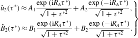
can be obtained from appropriate initial conditions. The solution for the amplitudes of
 $u_{2}^{\prime }$
,
 $B_{2}^{\prime }$
can then be written as
 $$\begin{eqnarray}\left.\begin{array}{@{}c@{}}\displaystyle \hat{u} _{2}(\unicode[STIX]{x1D70F}^{\ast })\approx A_{1}\frac{\exp (\text{i}R_{A}\unicode[STIX]{x1D70F}^{\ast })}{\sqrt{1+\unicode[STIX]{x1D70F}^{\ast 2}}}+A_{2}\frac{\exp (-\text{i}R_{A}\unicode[STIX]{x1D70F}^{\ast })}{\sqrt{1+\unicode[STIX]{x1D70F}^{\ast 2}}},\\ \displaystyle \hat{B}_{2}(\unicode[STIX]{x1D70F}^{\ast })\approx B_{1}\frac{\exp (\text{i}R_{A}\unicode[STIX]{x1D70F}^{\ast })}{\sqrt{1+\unicode[STIX]{x1D70F}^{\ast 2}}}+B_{2}\frac{\exp (-\text{i}R_{A}\unicode[STIX]{x1D70F}^{\ast })}{\sqrt{1+\unicode[STIX]{x1D70F}^{\ast 2}}}.\end{array}\right\}\end{eqnarray}$$
The behaviour of
 $u_{2}^{\prime },B_{2}^{\prime }$
is oscillatory, as a result of the dominating influence of harmonic exchange. Owing to pressure reorientation, the magnitude of
 $u_{2}^{\prime }$
and consequently
 $B_{2}^{\prime }$
decrease. Therefore, using Parseval’s theorem, the evolution of normal kinetic energy (
 $k_{2}$
) in physical space is given by
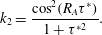 $$\begin{eqnarray}k_{2}=\frac{\cos ^{2}(R_{A}\unicode[STIX]{x1D70F}^{\ast })}{1+\unicode[STIX]{x1D70F}^{\ast 2}}.\end{eqnarray}$$
For the case of no initial magnetic field perturbations, the evolution of normal magnetic energy (
 $b_{2}$
) is given by
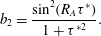 $$\begin{eqnarray}b_{2}=\frac{\sin ^{2}(R_{A}\unicode[STIX]{x1D70F}^{\ast })}{1+\unicode[STIX]{x1D70F}^{\ast 2}}.\end{eqnarray}$$
A solution to (3.50b
), similar to (3.55), was derived by Lau & Liu (Reference Lau and Liu1980). In this limit,
 $u_{2}^{\prime }$
and
 $B_{2}^{\prime }$
are oscillatory with a phase difference of
 $\unicode[STIX]{x03C0}/2$
and a time period of
 $T=2\unicode[STIX]{x03C0}/R_{A}$
. This oscillatory evolution results in negligible production and magnetic stretching when averaged over a full cycle. This implies that harmonic exchange between magnetic and kinetic energy dominates at all times. As a result, equipartition of energy between perturbation velocity and magnetic fields is indicated.
 $R_{A}\ll 1$
or low magnetic field limit. We first consider the evolution of the coefficients of the first terms on the right-hand sides of (3.50a
) and (3.50b
). At initial times,
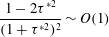 $$\begin{eqnarray}\frac{1-2\unicode[STIX]{x1D70F}^{\ast 2}}{(1+\unicode[STIX]{x1D70F}^{\ast 2})^{2}}\sim O(1)\end{eqnarray}$$
and asymptotes to zero at late times. Similarly, at early times,
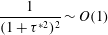 $$\begin{eqnarray}\frac{1}{(1+\unicode[STIX]{x1D70F}^{\ast 2})^{2}}\sim O(1)\end{eqnarray}$$
and asymptotes to zero at subsequent times. Thus, the first terms dominate during the early time in the low
 $R_{A}$
regime. At late times, however, the first terms have negligible contributions and the last terms dominate, i.e. harmonic exchange prevails. We now investigate the behaviour at early times.
Early-time behaviour. In this limit, the last terms in (3.50a
), (3.50b
) can be omitted. This implies that exchange is negligible and pressure reorientation is the crucial process at this stage. As a result, the evolution equations for
 $g,h$
can be written as follows:
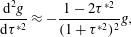 $$\begin{eqnarray}\displaystyle & \displaystyle \frac{\text{d}^{2}g}{\text{d}\unicode[STIX]{x1D70F}^{\ast 2}}\approx -\frac{1-2\unicode[STIX]{x1D70F}^{\ast 2}}{(1+\unicode[STIX]{x1D70F}^{\ast 2})^{2}}g, & \displaystyle\end{eqnarray}$$
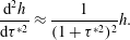 $$\begin{eqnarray}\displaystyle & \displaystyle \frac{\text{d}^{2}h}{\text{d}\unicode[STIX]{x1D70F}^{\ast 2}}\approx \frac{1}{(1+\unicode[STIX]{x1D70F}^{\ast 2})^{2}}h. & \displaystyle\end{eqnarray}$$
 $g$
equation (3.58a
) is identical to the pure hydrodynamic case, implying that the magnetic field does not affect the initial behaviour. The solution for such flows is given by
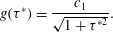 $$\begin{eqnarray}g(\unicode[STIX]{x1D70F}^{\ast })=\frac{c_{1}}{\sqrt{1+\unicode[STIX]{x1D70F}^{\ast 2}}}.\end{eqnarray}$$
The evolution of
 $k_{2}$
is given by
 $$\begin{eqnarray}k_{2}=\frac{1}{(1+\unicode[STIX]{x1D70F}^{\ast 2})^{2}}.\end{eqnarray}$$
The following is the analytical solution for
 $h,\hat{B}_{2}$
:
 $$\begin{eqnarray}h=\sqrt{1+\unicode[STIX]{x1D70F}^{\ast 2}}(c_{1}+c_{2}\arctan (\unicode[STIX]{x1D70F}^{\ast }))\Rightarrow \hat{B}_{2}=c_{1}+c_{2}\arctan (\unicode[STIX]{x1D70F}^{\ast }).\end{eqnarray}$$
If there is no initial magnetic field perturbation, then
 $c_{1}=0$
.
 $c_{2}$
can be determined from (3.46b
). Thus, the final solution for
 $b_{2}$
at early times is
 $$\begin{eqnarray}b_{2}=R_{A}^{2}\arctan ^{2}(\unicode[STIX]{x1D70F}^{\ast }).\end{eqnarray}$$
Late-time behaviour. For late times, harmonic exchange dominates as seen from the order of magnitude analysis performed above. As a result, the evolution of
 $\hat{u} _{2}$
and
 $\hat{B}_{2}$
becomes oscillatory, similar to the behaviour of cases with
 $R_{A}\gg 1$
.
Therefore,
 $u_{2}^{\prime }$
and
 $B_{2}^{\prime }$
for flows with
 $R_{A}\ll 1$
experience a three-stage evolution. At early times, pressure reorientation determines the dynamics. However, for later stages, harmonic exchange is the dominant mechanism. At late times, the equipartition between magnetic and kinetic energies is indicated once again. The behaviour at intermediate times where pressure reorientation and exchange are equally dominant will be deduced from numerical simulations.
3.2 Inferences from linear inviscid analysis
The following inferences can be made from inviscid linear analysis.
(i) For spanwise wavevector orientations, the velocity and magnetic field equations are decoupled leading to pressure-released behaviour. As a result,
$u_{1}^{\prime }$
grows linearly and
$u_{2}^{\prime },u_{3}^{\prime }$
remain unchanged. Consequently, kinetic energy grows quadratically. Since the exchange terms are zero, all the magnetic field components remain zero if not initialized.(ii) The behaviour of
$u_{2}^{\prime }$
and
$B_{2}^{\prime }$
is critical for other orientations,
$\unicode[STIX]{x1D6FD}\in [0^{\circ },90^{\circ })$
, as they determine the production and magnetic stretching processes, respectively.(iii) For the case of perturbations with
$R_{A}\ll 1$
,
$u_{2}^{\prime }$
and
$B_{2}^{\prime }$
exhibit a three-stage behaviour. At early times, the evolution resembles that of incompressible hydrodynamic flows. Subsequently, the kinetic–magnetic harmonic exchange dominates. This results in oscillatory evolution of
$u_{2}^{\prime }$
and
$B_{2}^{\prime }$
at late times.(iv) For perturbations with
$R_{A}\gg 1$
, harmonic kinetic–magnetic exchange dominates and the evolution is oscillatory from the beginning.(v) At late times, irrespective of
$R_{A}$
, harmonic exchange between kinetic and magnetic energies dominate, leading to equipartition of energy.(vi) The effect of
$\unicode[STIX]{x1D6FD}$
is to merely influence the timescale of evolution. With increasing
$\unicode[STIX]{x1D6FD}$
, the kinetic–magnetic coupling becomes weaker and the evolution rate progressively slows down.


In the following sections, we investigate the validity of the derived closed-form analytical solutions and the above inferences. For this assessment, we perform numerical simulations of nonlinear, viscous, resistive MHD equations.
4 Numerical setup
DNS performed in this study employ the magneto-gas kinetic scheme (MGKM) developed by Araya et al. (Reference Araya, Ebersohn, Anderson and Girimaji2015). MGKM utilizes the kinetic-based gas kinetic method (GKM) for solving the flow field equations. The magnetic field is computed from Ohm’s law using a finite-difference solver. Lorentz force and Joule heating terms are added as source terms in the momentum and energy equations, respectively. The GKM portion of the scheme has been exhaustively validated in Kumar et al. (Reference Kumar, Bertsch and Girimaji2014) for homogeneous shear turbulence, Xie & Girimaji (Reference Xie and Girimaji2014) for wall-bounded flows and Karimi & Girimaji (Reference Karimi and Girimaji2016) for free shear flows. The details of the numerical scheme and validation for the case of shock tube and channel flow simulations are described in Araya et al. (Reference Araya, Ebersohn, Anderson and Girimaji2015).
The schematic of the background velocity and magnetic fields with perturbations is shown in figure 1(a). Periodic boundary conditions are applied in streamwise and spanwise directions. For boundaries in normal direction, shear periodic boundary conditions are applied (Baron Reference Baron1982):
 $$\begin{eqnarray}\unicode[STIX]{x1D719}(t,x+m_{1}L_{1},y+m_{2}L_{2},z+m_{3}L_{3})=\unicode[STIX]{x1D719}(t,x-Sm_{2}L_{2}t,y,z),\end{eqnarray}$$
where
 $L_{2}$
is the length of the domain in the normal direction and
 $m_{1},m_{2},m_{3}$
are integers.
Simulation parameters.
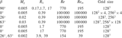
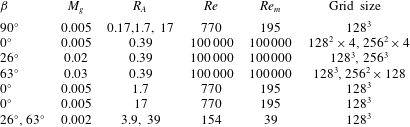
Simulations are performed for different shear-to-magnetic timescales (
 $R_{A}$
). Table 1 lists the details of various simulations. As
 $u_{2}^{\prime }$
is the most critical for the development of fluid instabilities, only these perturbations are considered in the initial conditions:
 $$\begin{eqnarray}u_{1}^{\prime }(0)=0,\quad u_{2}^{\prime }(0)=\sin (\unicode[STIX]{x1D705}_{1}x_{1}+\unicode[STIX]{x1D705}_{3}x_{3}),\quad u_{3}^{\prime }(0)=0,\end{eqnarray}$$
 $$\begin{eqnarray}B_{1}^{\prime }(0)=0,\quad B_{2}^{\prime }(0)=0,\quad B_{3}^{\prime }(0)=0,\end{eqnarray}$$
where
 $\unicode[STIX]{x1D705}_{1}$
and
 $\unicode[STIX]{x1D705}_{3}$
are integers and
 $\unicode[STIX]{x1D705}_{1}$
and
 $\unicode[STIX]{x1D705}_{3}$
are modified such that the perturbation wavevector orientations vary from streamwise to spanwise directions, i.e.
 $\unicode[STIX]{x1D6FD}\in [0^{\circ },90^{\circ }]$
. Reynolds numbers, fluid and magnetic (
 $\mathit{Re}=S/\unicode[STIX]{x1D708}\unicode[STIX]{x1D705}^{2},\mathit{Re}_{m}=S/\unicode[STIX]{x1D702}\unicode[STIX]{x1D705}^{2}$
) and
 $\unicode[STIX]{x1D6FD}$
values considered in different simulations are listed in table 1. Since MGKM is a compressible flow solver, we choose low gradient Mach numbers,
 $M_{g}\equiv S/\unicode[STIX]{x1D705}a\leqslant 0.03$
, to emulate the incompressible limit. A grid sensitivity study is performed for the case of
 $\unicode[STIX]{x1D6FD}=0^{\circ }$
in the low
 $R_{A}~(=0.39)$
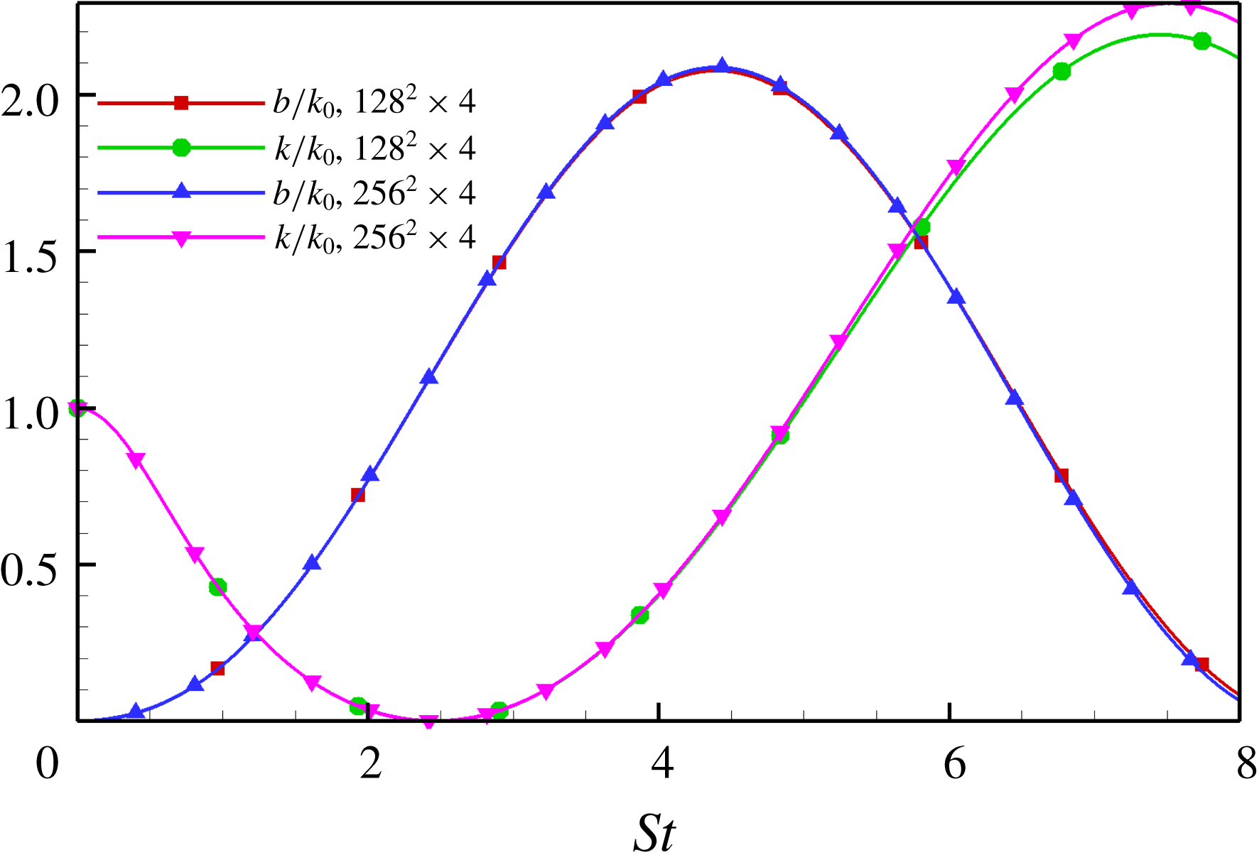
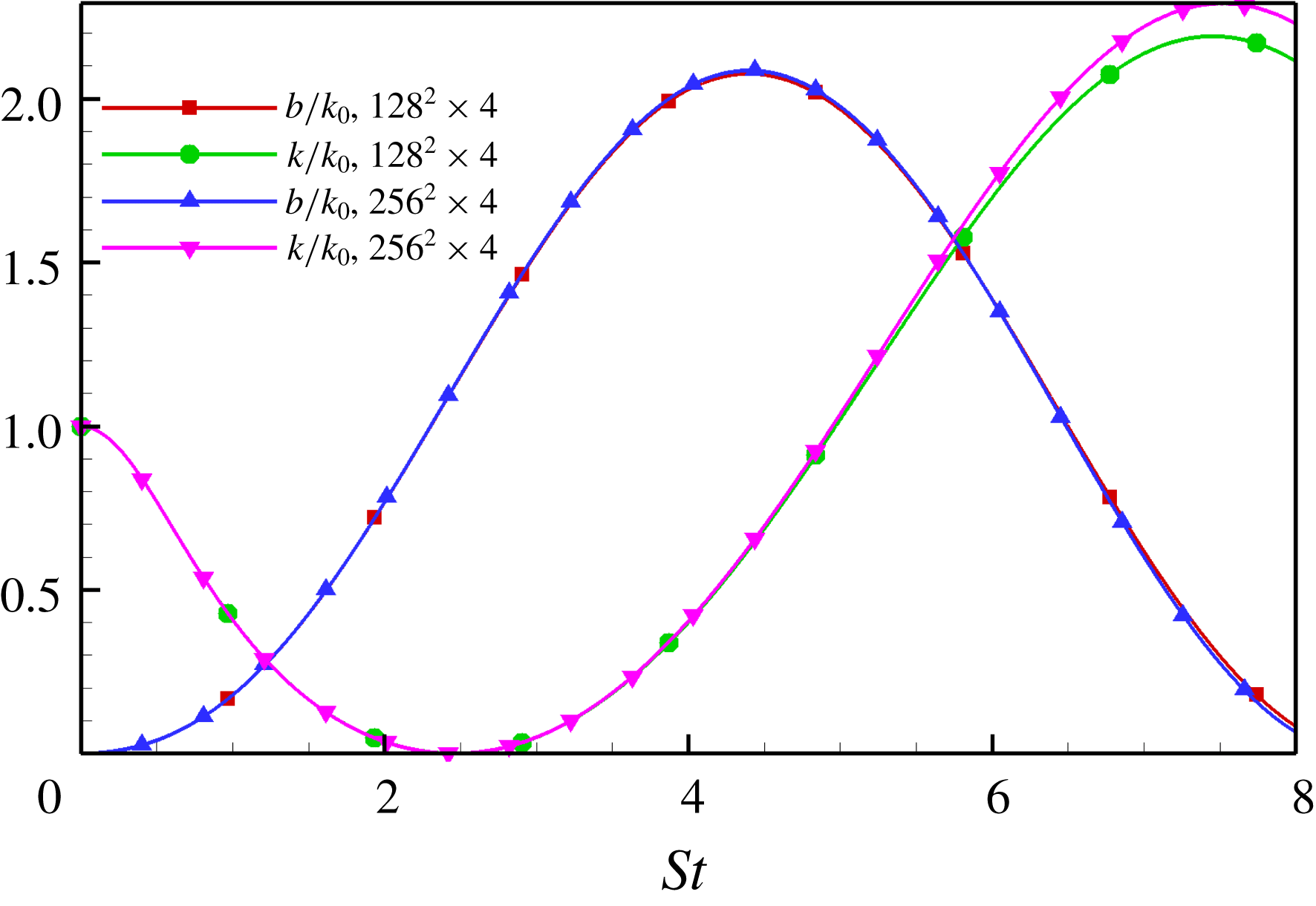
limit. Figure 2 shows that
 $128\times 128\times 4$
and
 $256\times 256\times 4$
give nearly identical results except for a higher numerical dissipation in the low-resolution simulation. As the evolution of long-wavelength perturbations is of current interest, the grid resolution requirements are much less stringent than turbulent flows. The smallest energetic wavelength encountered at the end of the run is of the order of the domain size. Thus, the grid resolution employed in the simulation is quite adequate. Nonlinear breakdown and transition to turbulence would require much finer grids and such investigation is currently underway. The analytical results derived in the previous sections would validate the implementation of shear periodic boundary conditions into MGKM for future nonlinear studies.
Grid independence for
 $R_{A}=0.39$
and
 $\unicode[STIX]{x1D6FD}=0^{\circ }$
.
In addition to DNS, the RDT equations (3.22) and (3.23) are evolved temporally using a fourth-order Runge–Kutta method. To contrast the MHD flow evolution against hydrodynamic flows, cases with
 $R_{A}=0$
are also considered. Analytical results and numerical solutions from RDT and DNS are compared in the next section.
5 Results
We now present simulation results for various cases of
 $R_{A}$
and perturbation wavevector orientations. As listed in table 1, for a given value of
 $\unicode[STIX]{x1D6FD}$
different magnetic field strengths are considered to correspond to low, intermediate and high magnetic field effects. We use the notation introduced in (3.30a–h
) to refer to different components of normalized kinetic and magnetic energies. Throughout MRDT refers to temporally evolved solutions of (3.22) and (3.23), whereas HRDT refers to the hydrodynamic effect alone. We now present the results of spanwise fluctuations and then for other orientations.
Spanwise perturbations –
 $\unicode[STIX]{x1D737}=90^{\circ }$
. This perturbation orientation (
 $\cos \unicode[STIX]{x1D6FD}=0$
) represents a special limit as velocity and magnetic fields are decoupled. In addition, the velocity fields are impervious to pressure (3.40a–c
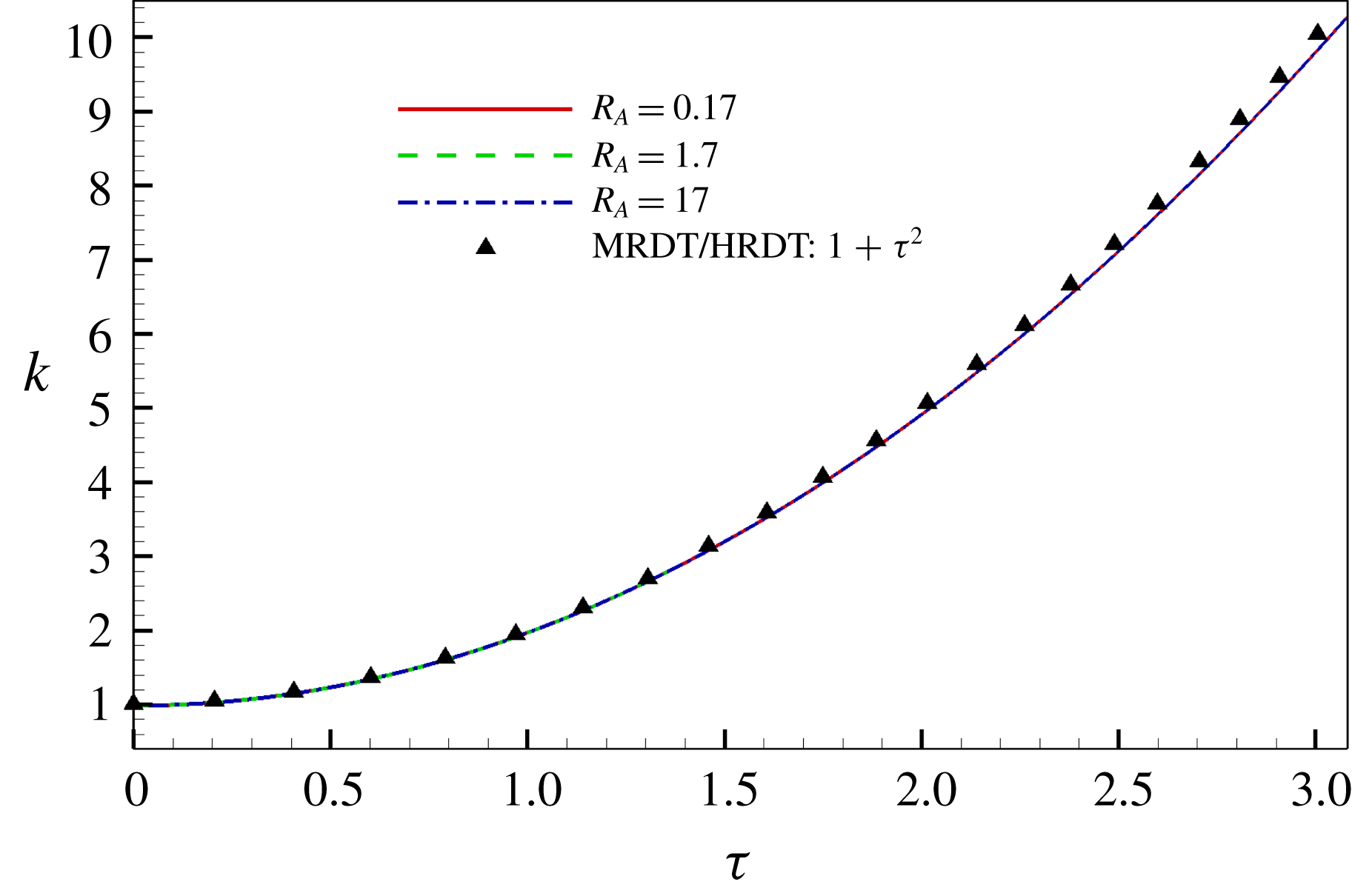
). The evolution of kinetic energy (
 $k$
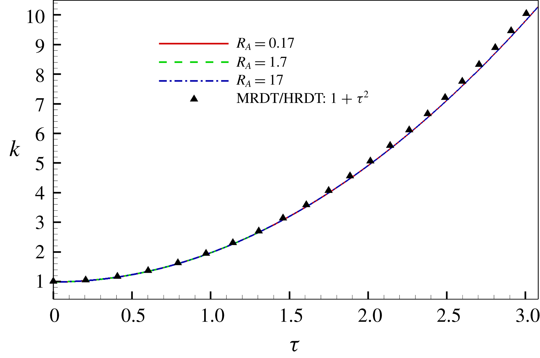
) at different magnetic fields is plotted in figure 3. It can be seen that
 $k$
grows quadratically, consistent with the MRDT and HRDT analytical solution given in (3.42), regardless of the magnetic field strength. This confirms that the flow field behaves in accordance to the pressure-released hydrodynamic equations noted in § 3.1.1. For the initial conditions considered, perturbation magnetic energy remains zero at all times, for all background magnetic field strengths.
Spanwise perturbation: evolution of kinetic energy,
 $k$
, of
 $R_{A}=0.17,1.7$
and
 $17$
compared against pressure-released hydrodynamic solution of MRDT
 $k=1+\unicode[STIX]{x1D70F}^{2}$
.
Perturbations with
 $\unicode[STIX]{x1D737}\in [\!0^{\circ },90^{\circ }\!)$
. The results for low, intermediate and high magnetic field cases are now presented for other wavevector orientations.
5.1 Low magnetic field regime,
$R_{A}\ll 1$

Linear analysis suggests a three-stage behaviour for
 $R_{A}\ll 1$
cases. The different stages are now examined.
Early hydrodynamic behaviour (
 $\unicode[STIX]{x1D70F}^{\ast }<1$
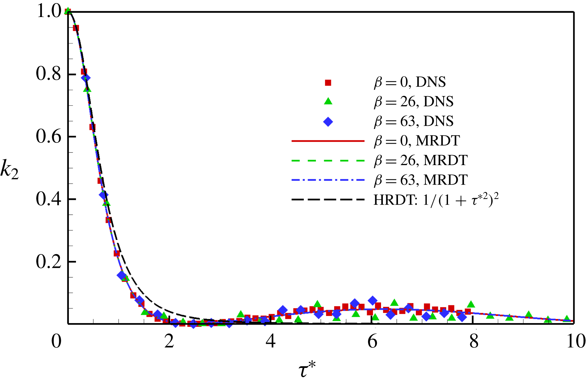
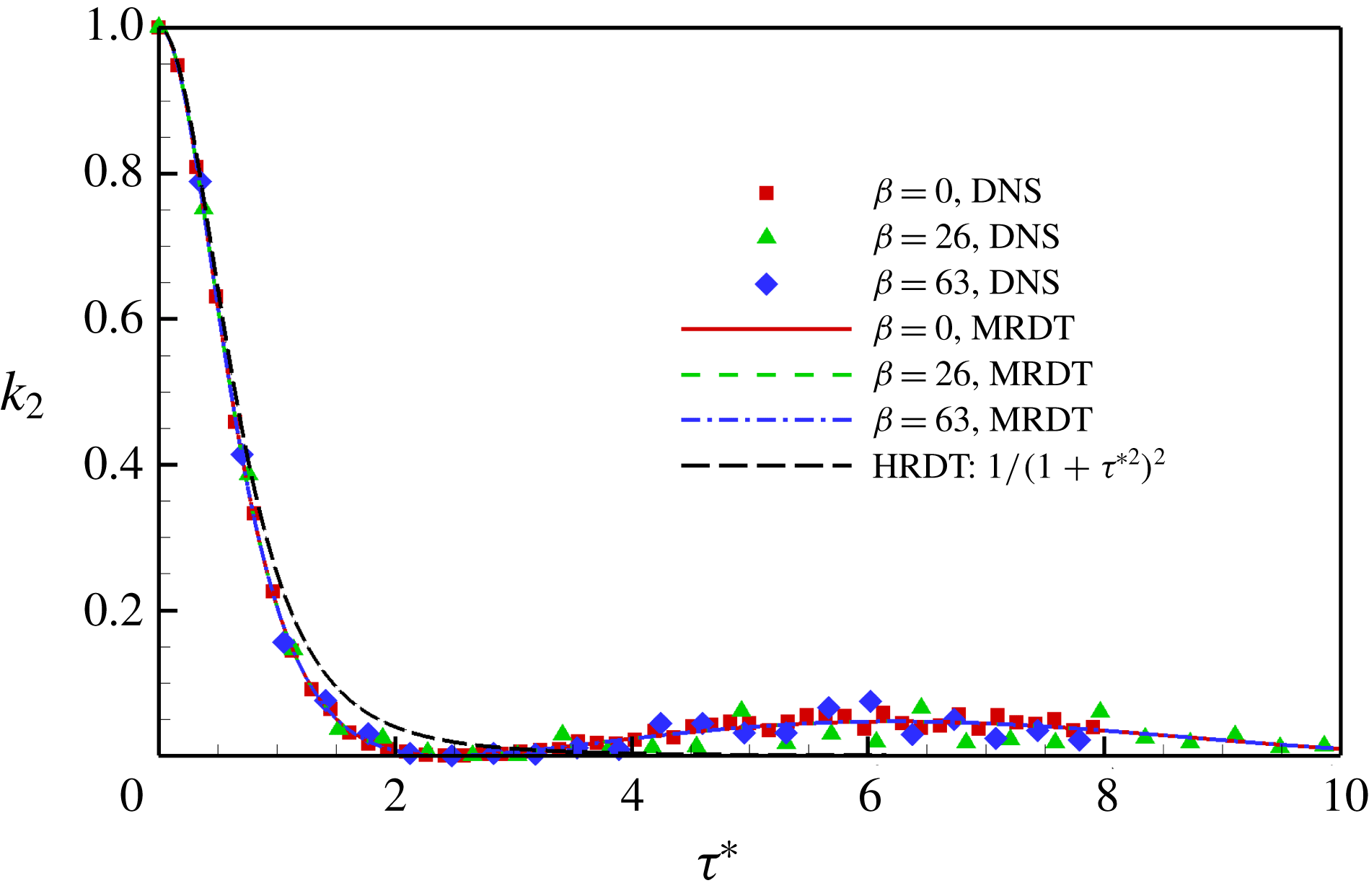
). Figure 4 presents the behaviour of
 $k_{2}$
for the case of
 $R_{A}=0.39$
and various
 $\unicode[STIX]{x1D6FD}$
values. The analytical result (3.60) is compared against numerical solutions of MRDT and DNS. The self-similarity of
 $k_{2}$
evolution is clearly evident. Since only
 $k_{2}$
is initialized in DNS and RDT, the dominant processes in this stage are pressure redistribution and production. For
 $\unicode[STIX]{x1D6FD}=0^{\circ },26^{\circ }$
, the action of pressure redistributes
 $k_{2}$
to
 $k_{1}$
and
 $k_{3}$
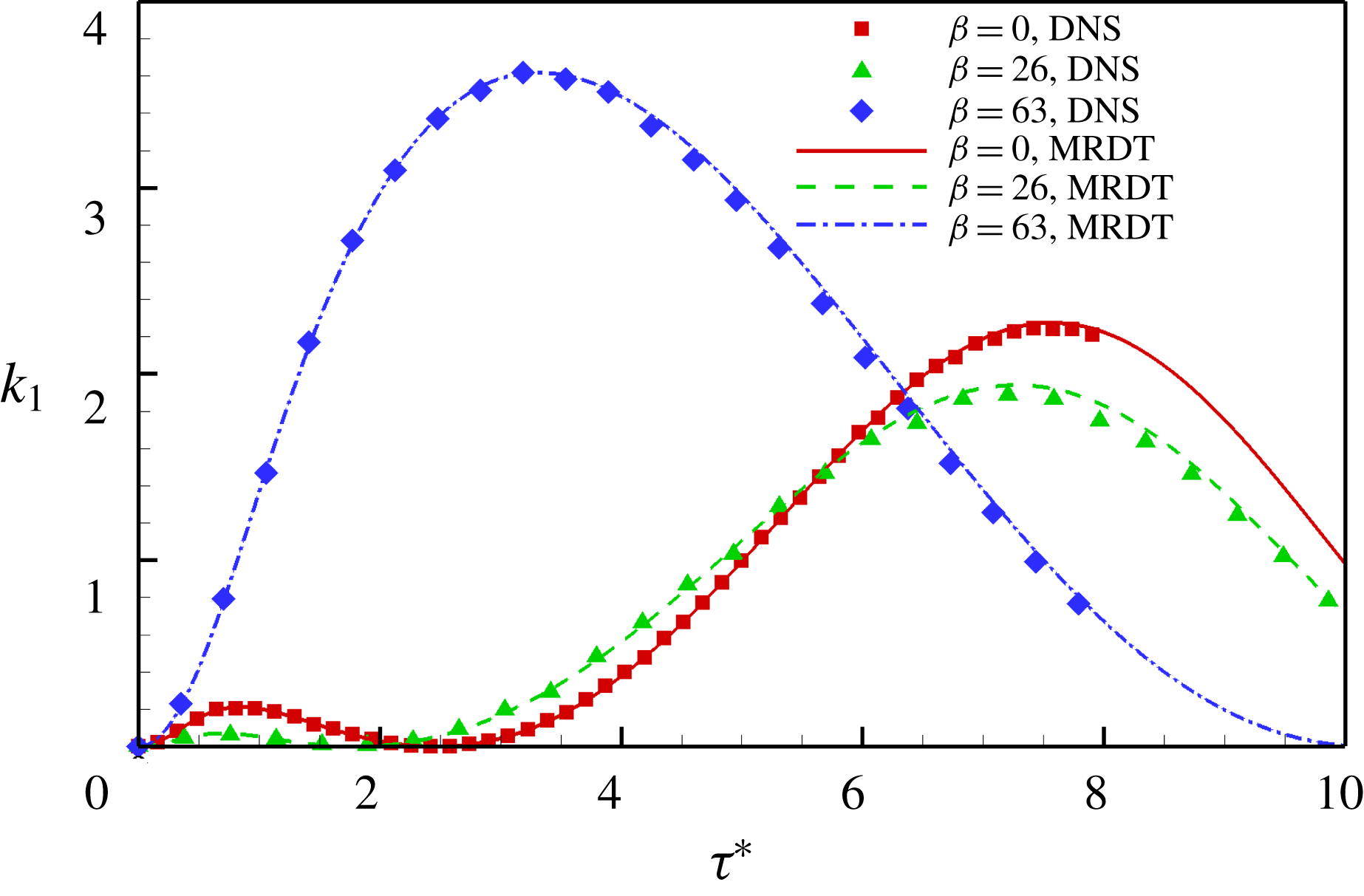
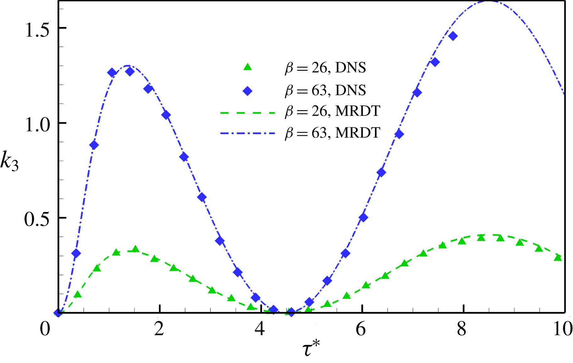
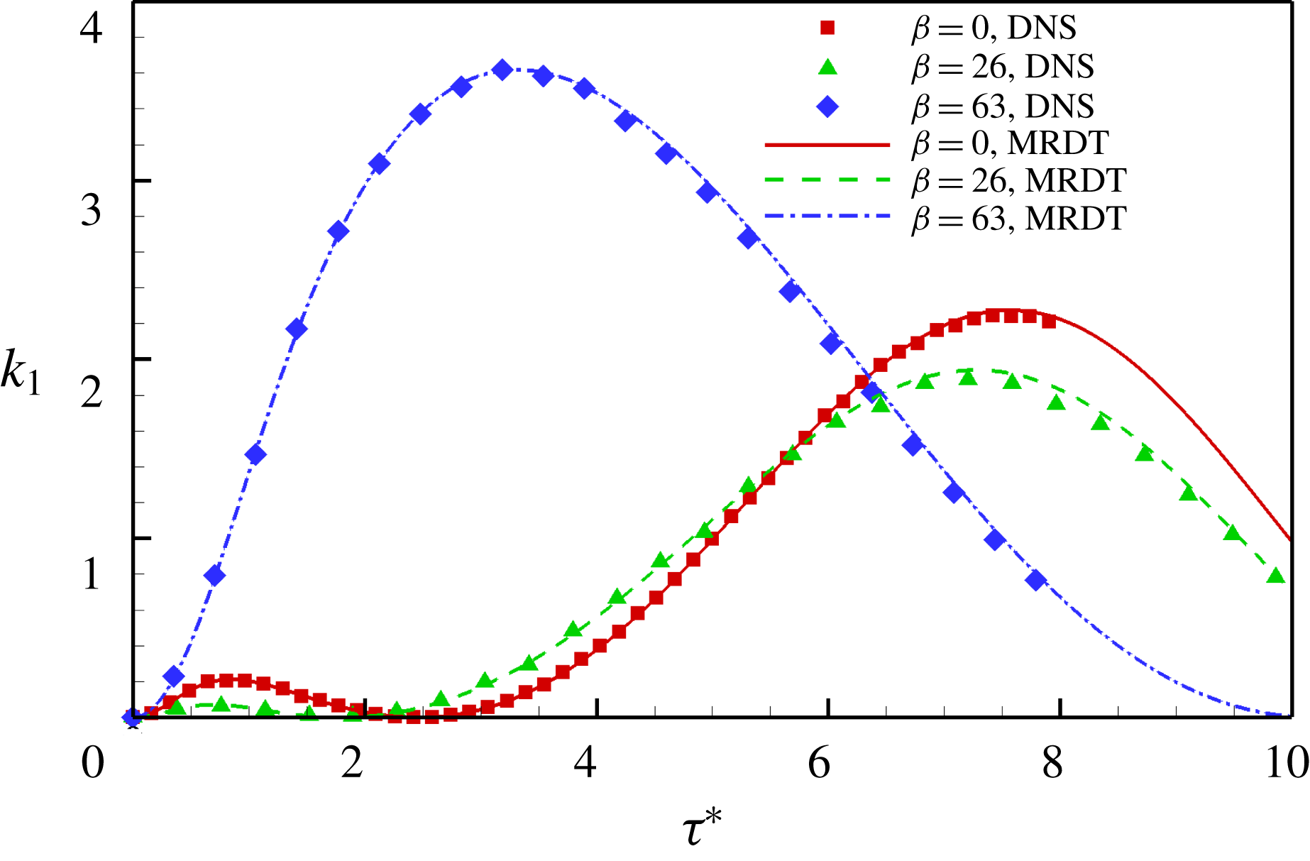
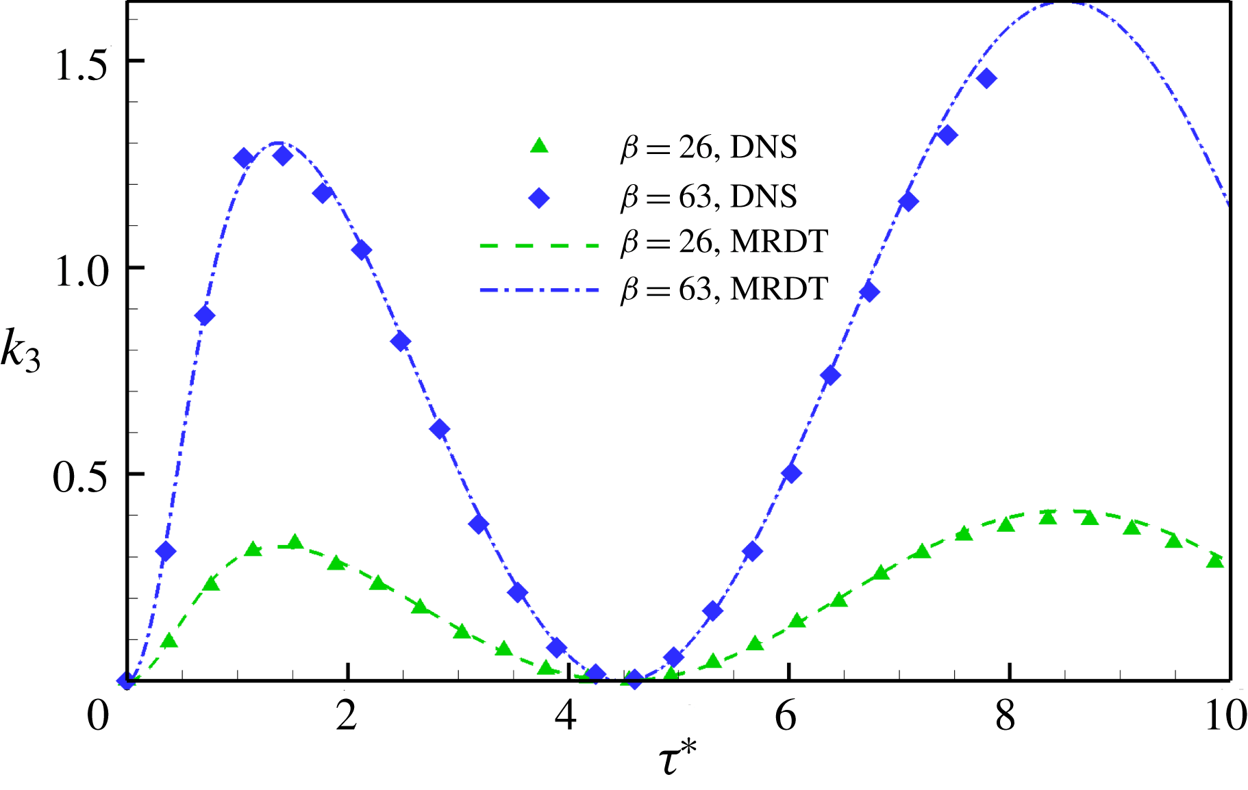
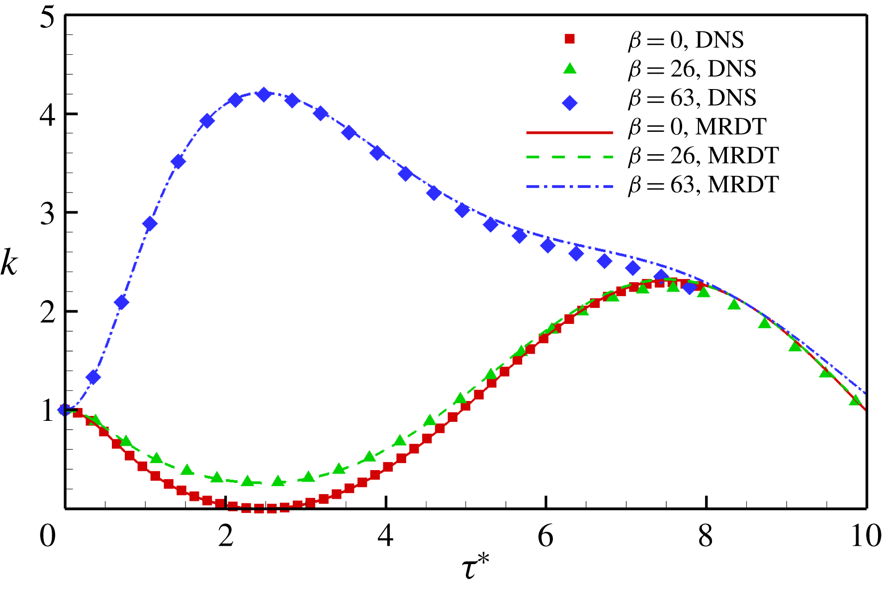
as seen from the increase in their values in figures 5 and 6. This implies that production of
 $k_{1}$
is negative for
 $\unicode[STIX]{x1D6FD}=0^{\circ },26^{\circ }$
in the first stage. For
 $\unicode[STIX]{x1D6FD}=63^{\circ }$
,
 $u_{1}^{\prime }$
and
 $u_{2}^{\prime }$
are negatively correlated; as a result,
 $k_{1}$
increases owing to production and pressure redistributes energy from
 $k_{1}$
to
 $k_{2}$
and
 $k_{2}$
to
 $k_{3}$
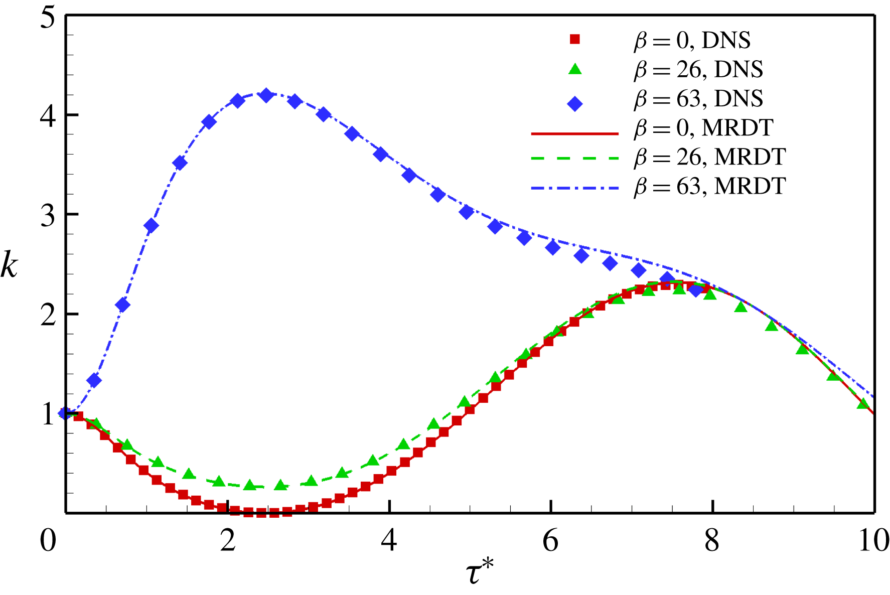
. The evolution of
 $k$
in figure 7 also proves that production is negative for
 $\unicode[STIX]{x1D6FD}=0^{\circ },26^{\circ }$
and positive for
 $63^{\circ }$
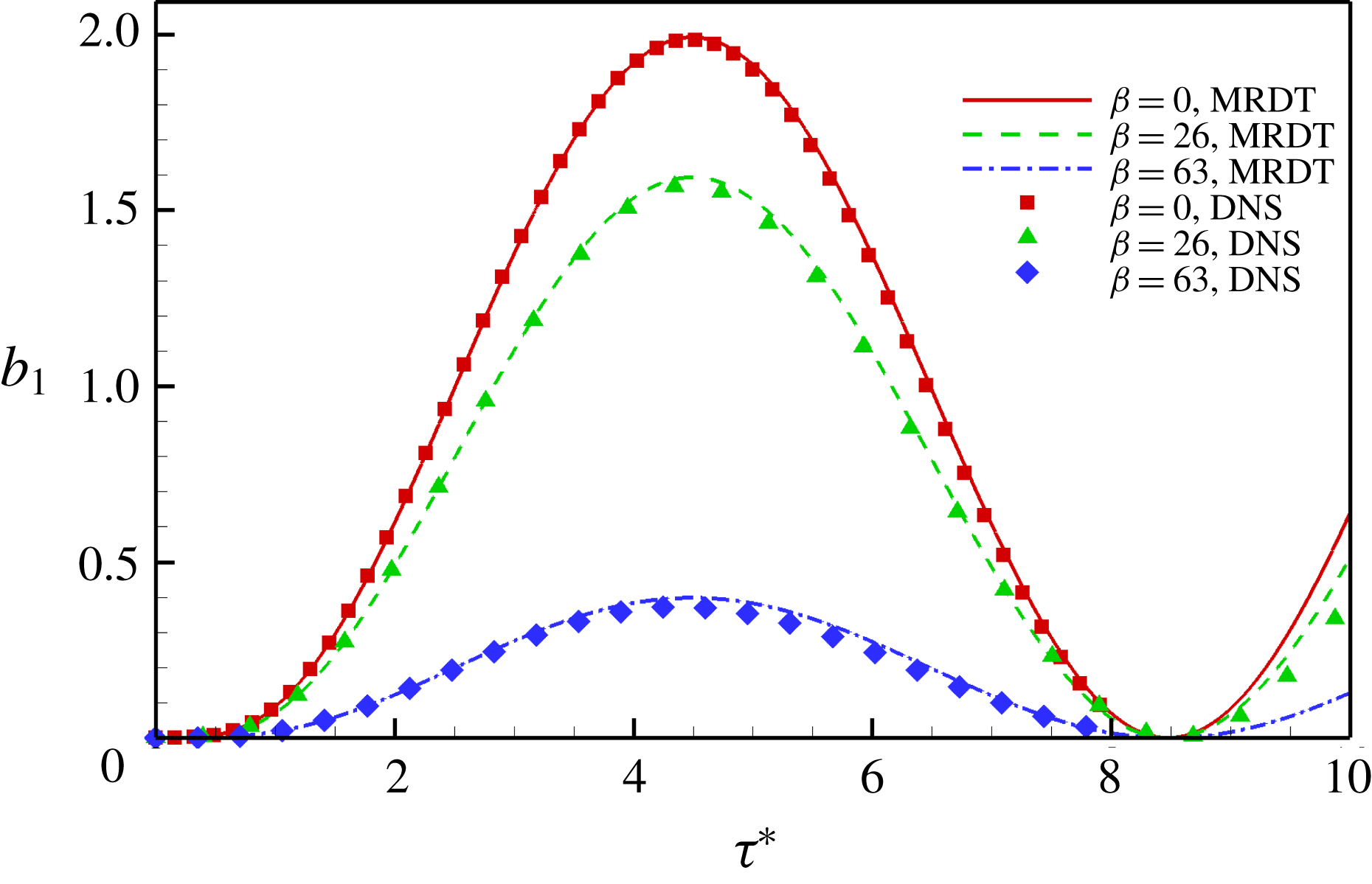
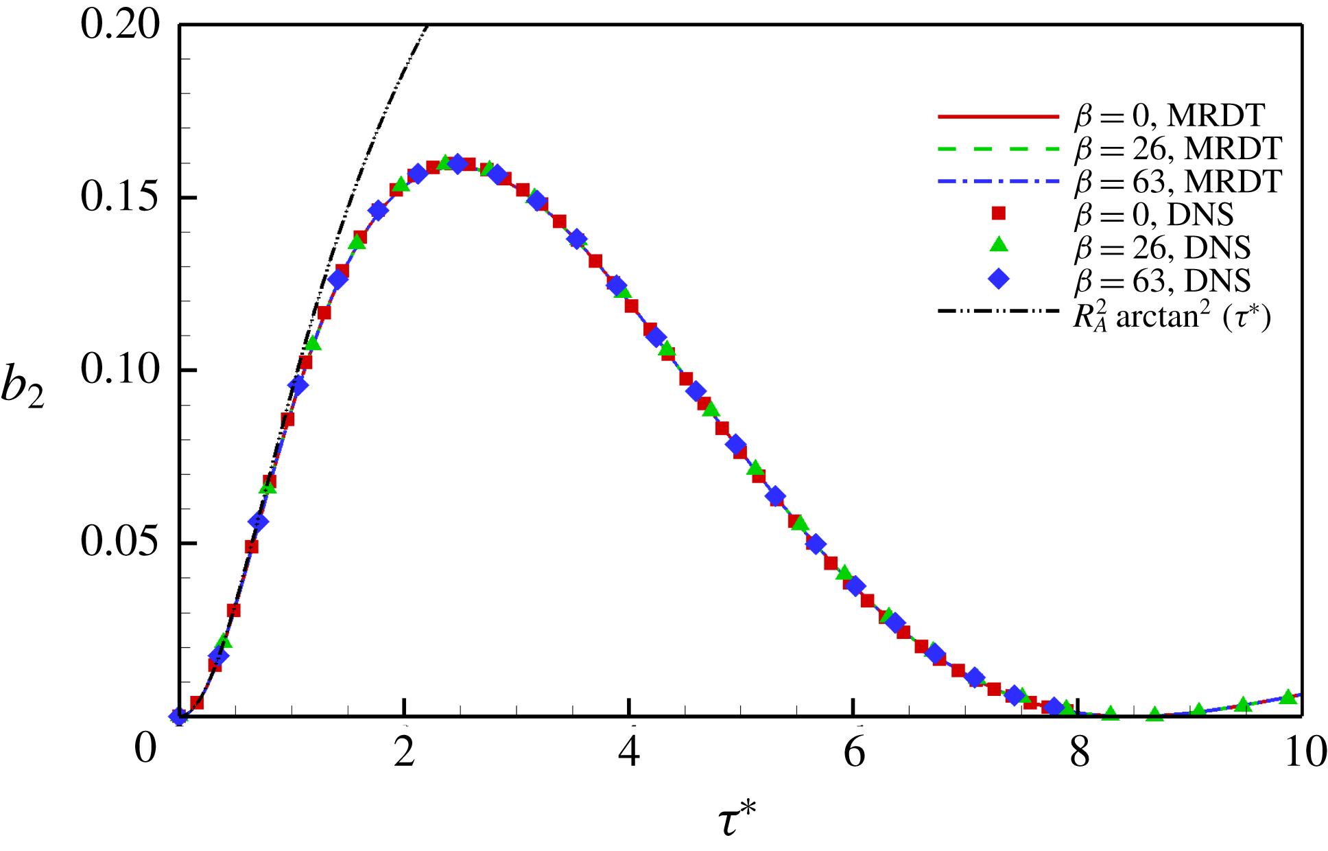
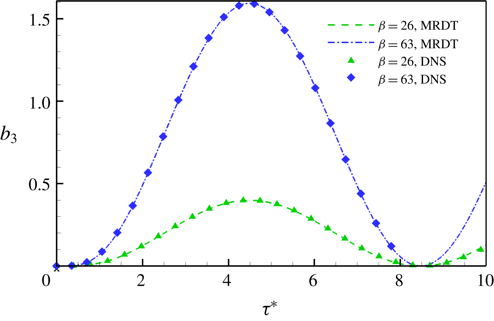
. There is a small amount of energy transfer from velocity field to their respective magnetic field components as is evident from the evolution of
 $b_{1}$
,
 $b_{2}$
and
 $b_{3}$
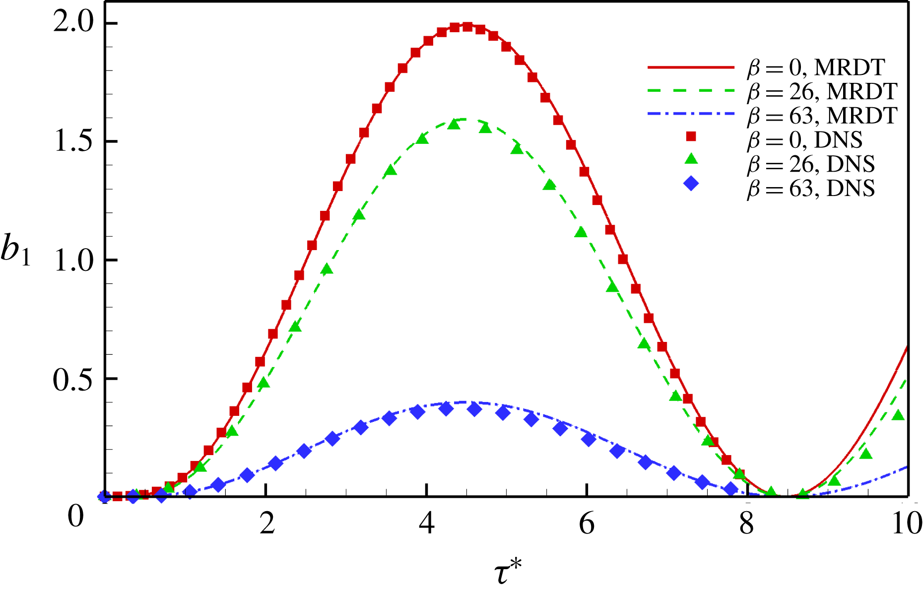
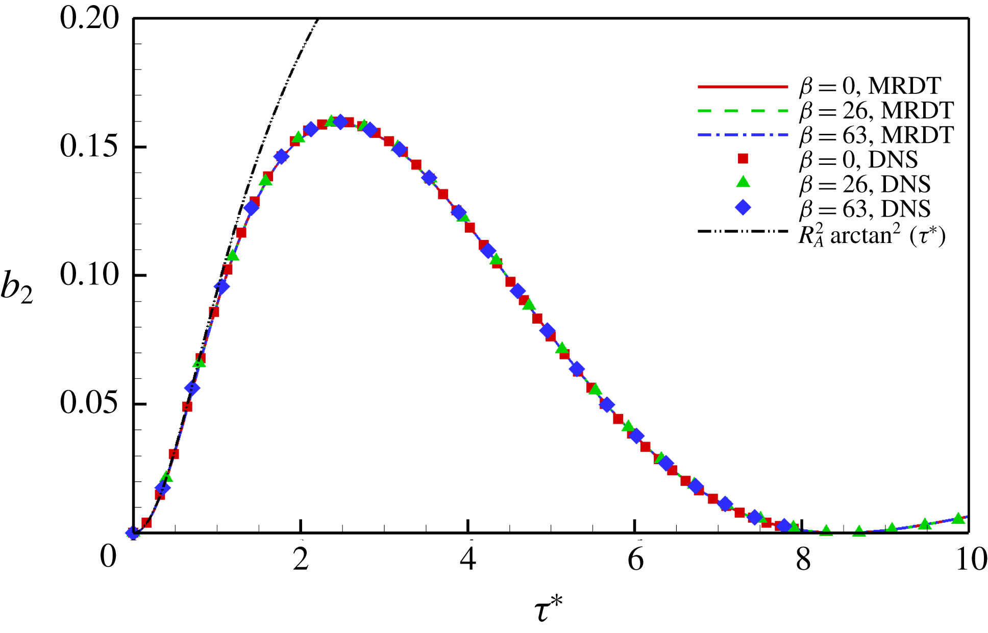
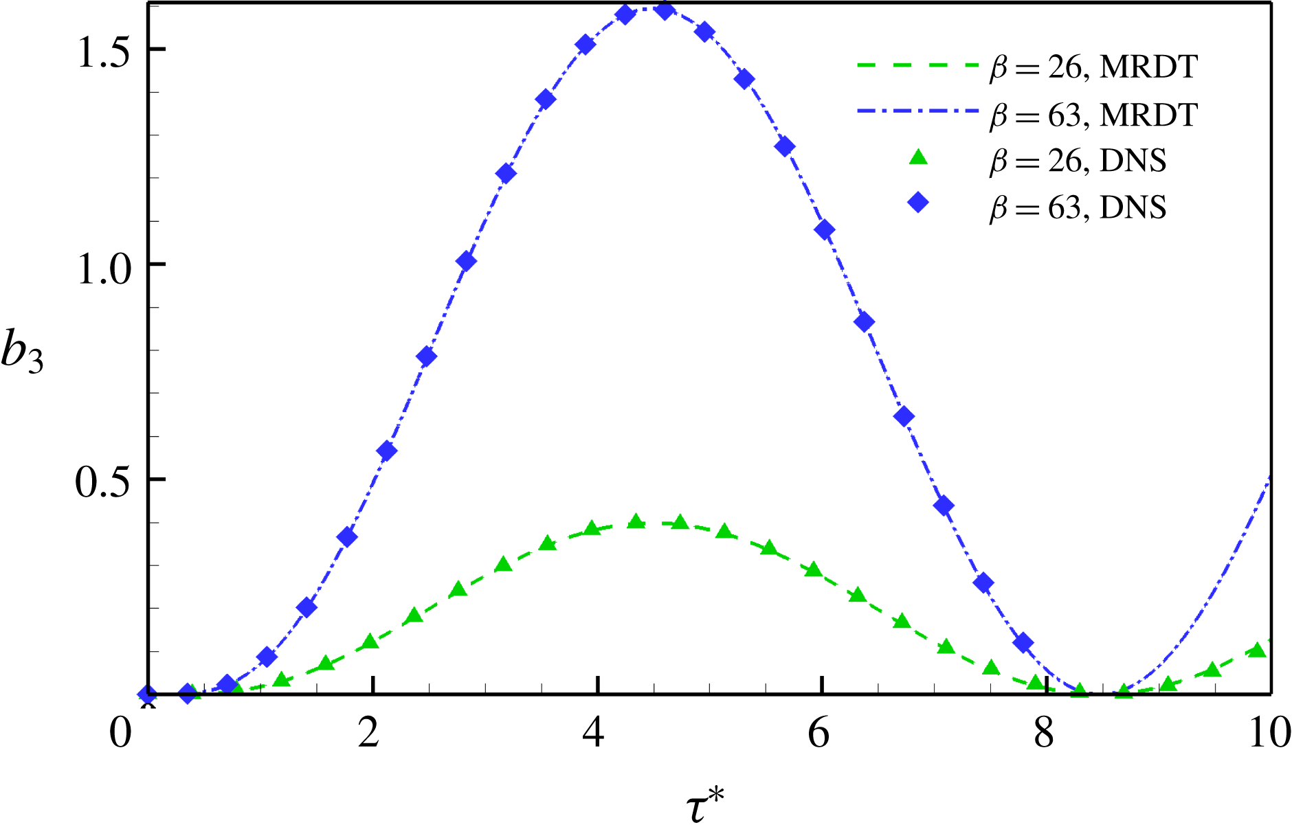
in figures 8, 9 and 10, respectively. The linear-inviscid analytical solution for
 $b_{2}$
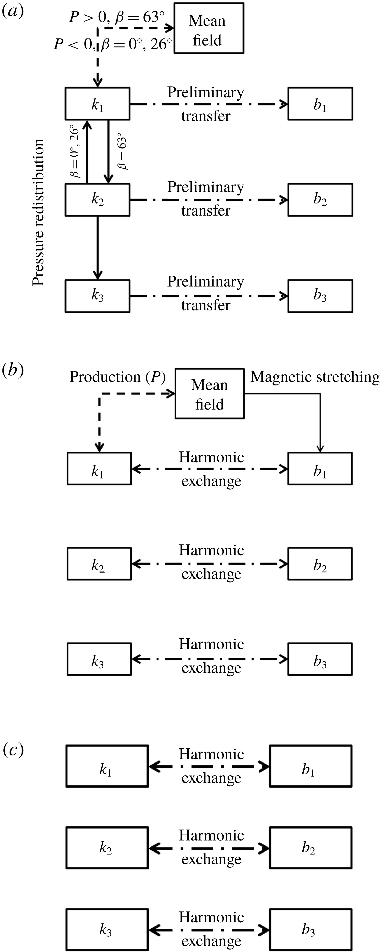
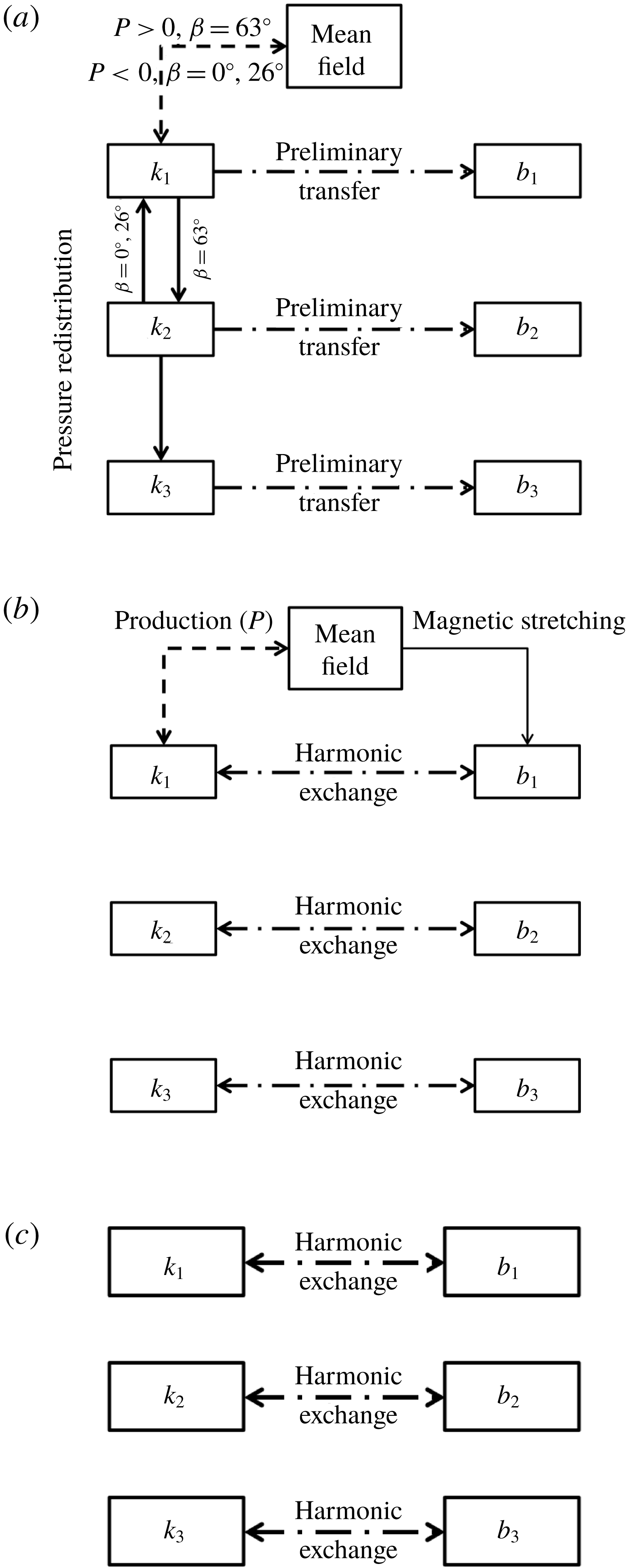
given in (3.62) is compared against DNS and MRDT in figure 9 and demonstrates good agreement. Figure 11(a) is a schematic that identifies the various energy exchanges dominant at the early stages. Clearly, the velocity field behaviour in this regime is very similar to the hydrodynamic case as evidenced by the negligible transfer of energy to the magnetic field.
Low
 $R_{A}$
regime (
 $R_{A}=0.39$
): evolution of
 $k_{2}$
obtained using DNS and MRDT for
 $\unicode[STIX]{x1D6FD}=0^{\circ },26^{\circ },63^{\circ }$
compared against the analytical solution of HRDT
 $k_{2}=1/(1+\unicode[STIX]{x1D70F}^{\ast 2})^{2}$
.
Low
 $R_{A}$
regime (
 $R_{A}=0.39$
): evolution of
 $k_{1}$
obtained using DNS and MRDT for
 $\unicode[STIX]{x1D6FD}=0^{\circ },26^{\circ },63^{\circ }$
.
Low
 $R_{A}$
regime (
 $R_{A}=0.39$
): evolution of
 $k_{3}$
obtained using DNS and MRDT for
 $\unicode[STIX]{x1D6FD}=26^{\circ },63^{\circ }$
. For
 $\unicode[STIX]{x1D6FD}=0^{\circ }$
,
 $k_{3}=0$
at all times.
Low
 $R_{A}$
regime (
 $R_{A}=0.39$
): kinetic energy (
 $k$
) evolution obtained using DNS and MRDT for
 $\unicode[STIX]{x1D6FD}=0^{\circ },26^{\circ },63^{\circ }$
.
Low
 $R_{A}$
regime (
 $R_{A}=0.39$
): evolution of
 $b_{1}$
obtained using DNS and MRDT for
 $\unicode[STIX]{x1D6FD}=0^{\circ },26^{\circ },63^{\circ }$
.
Low
 $R_{A}$
regime (
 $R_{A}=0.39$
): evolution of
 $b_{2}$
obtained using DNS and MRDT for
 $\unicode[STIX]{x1D6FD}=0^{\circ },26^{\circ },63^{\circ }$
compared against the analytical solution
 $b_{2}=R_{A}^{2}\arctan ^{2}(\unicode[STIX]{x1D70F}^{\ast })$
.
Low
 $R_{A}$
regime (
 $R_{A}=0.39$
): evolution of
 $b_{3}$
obtained using RDT and DNS for
 $\unicode[STIX]{x1D6FD}=0^{\circ },26^{\circ },63^{\circ }$
.
Low
 $R_{A}$
regime: schematic of dominant processes. (a) Dominant processes in stage 1: pressure redistribution (solid) and production
 $P$
(dashed). (b) Dominant processes in stage 2: production, magnetic stretching and harmonic exchange. (c) Dominant processes in stage 3: harmonic exchange.
Intermediate stage onset of magnetic field effect. For
 $\unicode[STIX]{x1D70F}^{\ast }\geqslant 1$
, the magnetic field processes set in. The small amount of energy transfer to
 $b_{1}$
and
 $b_{2}$
in the first stage seeds the growth of perturbation magnetic energy (
 $b$
) owing to magnetic stretching. This growth can be seen from the significant increase of
 $b_{1}$
(figure 8) for the case of
 $\unicode[STIX]{x1D6FD}=0^{\circ }$
. The increase cannot solely be attributed to harmonic exchange with
 $k_{1}$
, since
 $k_{1}$
values never exceed unity for this case, proving that this is a consequence of magnetic stretching. From figure 4,
 $k_{2}$
goes to zero faster than the hydrodynamic case as a result of exchange with
 $b_{2}$
. At
 $\unicode[STIX]{x1D70F}^{\ast }\approx 2$
,
 $k_{2}$
goes to zero. Subsequently,
 $k_{2}$
starts growing again owing to harmonic exchange with
 $b_{2}$
. Similarly,
 $k_{1}$
(figure 5) increases for
 $\unicode[STIX]{x1D6FD}=0^{\circ },26^{\circ }$
and decreases for
 $\unicode[STIX]{x1D6FD}=63^{\circ }$
owing to harmonic exchange with
 $b_{1}$
. Harmonic exchange is the only dominant process for the velocity and magnetic field perturbations in the spanwise direction, and the transfer is from
 $k_{3}$
to
 $b_{3}$
. The growth of magnetic perturbations along the streamwise direction in this stage is the amplification identified in Chagelishvili et al. (Reference Chagelishvili, Hristov, Chanishvili and Lominadze1993) and Dimitrov et al. (Reference Dimitrov, Maneva, Hristov and Mishonov2011). The exchange dynamics of this stage are summarized in figure 11(b).
Late stage behaviour. For times
 $\unicode[STIX]{x1D70F}^{\ast }>4$
, the only dominant linear process is the harmonic exchange between the corresponding velocity and magnetic field components. The oscillations of
 $u_{2}^{\prime }$
and
 $B_{2}^{\prime }$
about zero cause the sum of kinetic energy production and magnetic energy stretching production to vanish when integrated over a cycle. The magnetic and kinetic fields harmonically exchange energies with a time period of
 $\unicode[STIX]{x03C0}/R_{A}$
for the case of
 $\unicode[STIX]{x1D6FD}=0^{\circ },26^{\circ },63^{\circ }$
. Slight deviations from the analytical MRDT solutions are attributed to the numerical dissipation and compressibility effects present in DNS. The presence of numerical dissipation is also evident in the grid independence study demonstrated in figure 2. The linear energy interaction processes in this stage of evolution are summarized in figure 11(c).
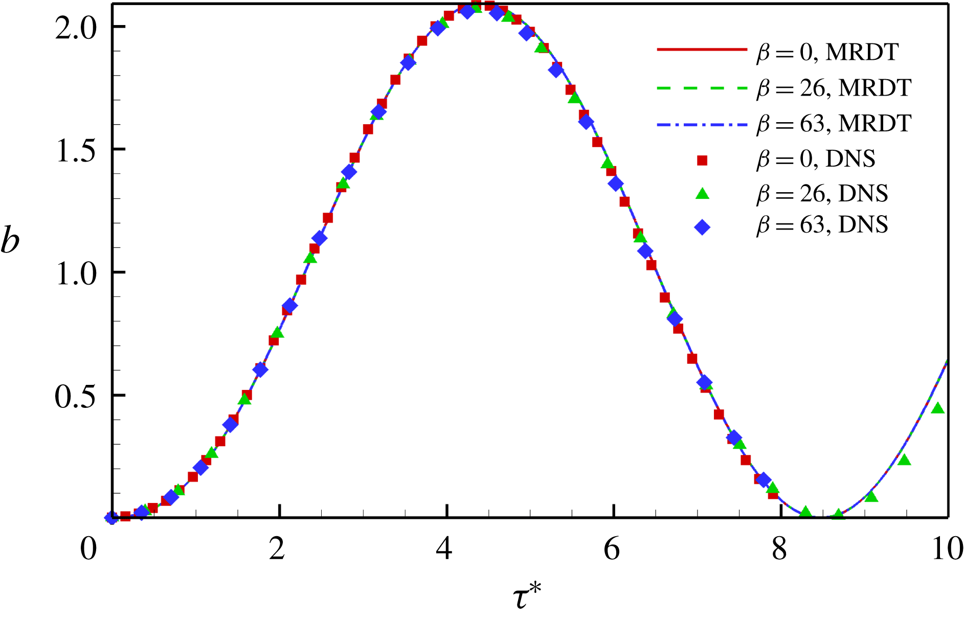
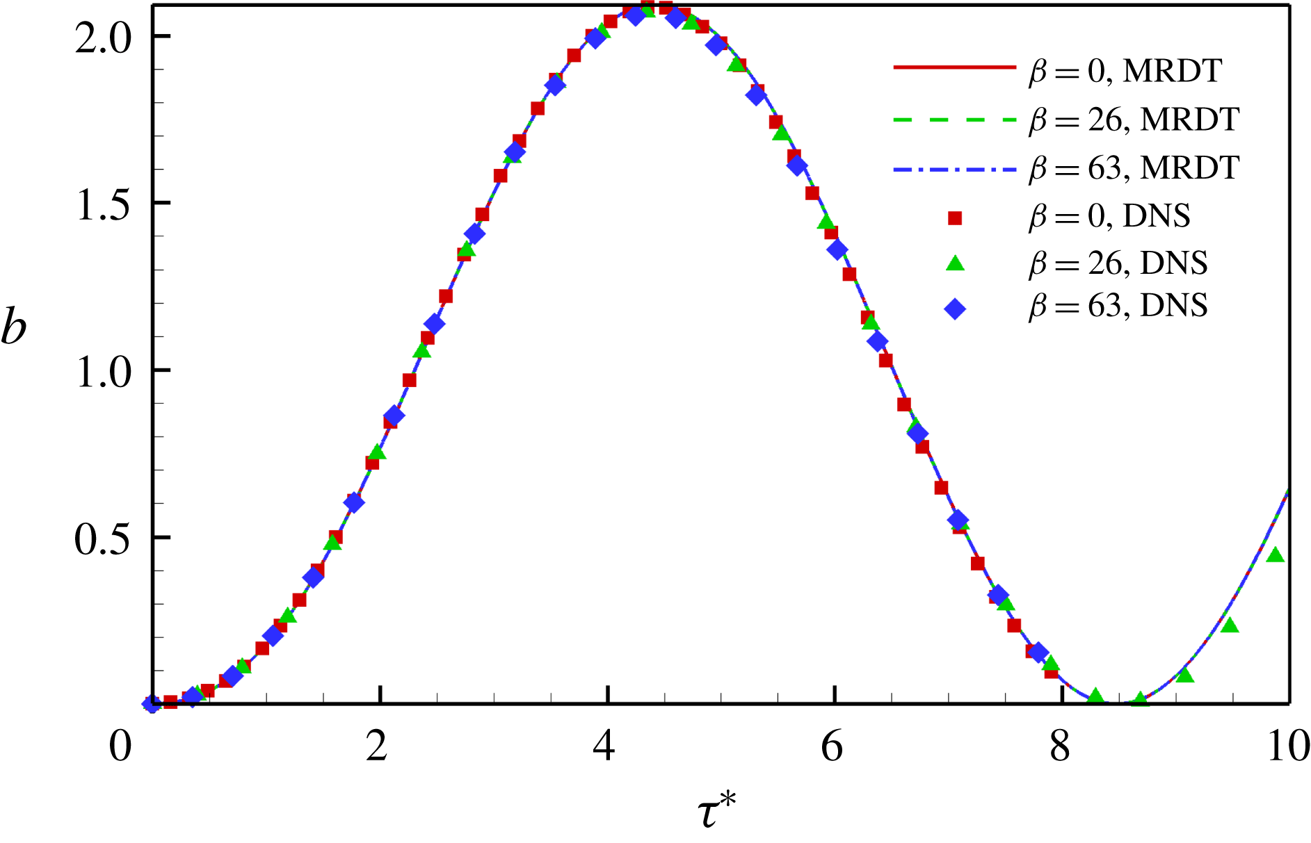
Some important observations can be made about the evolution of magnetic energy (
 $b$
) seen in figure 12. For a given
 $R_{A}$
,
 $b$
experiences a self-similar evolution (figure 12) in the linear stage at all
 $\unicode[STIX]{x1D6FD}$
in spite of magnetic stretching occurring on the shear (
 $S$
) timescale. This is due to the fact that
 $b_{2}$
is initially zero in both DNS and RDT. The
 $b_{2}$
responsible for magnetic stretching is generated owing to exchange from
 $k_{2}$
. Since the transfer from
 $k_{2}$
to
 $b_{2}$
occurs on magnetic (
 $V_{A}\unicode[STIX]{x1D705}_{0}\cos \unicode[STIX]{x1D6FD}$
) timescale, for a given
 $R_{A}$
,
 $b$
experiences a self-similar evolution for all
 $\unicode[STIX]{x1D6FD}$
in scaled time
 $\unicode[STIX]{x1D70F}^{\ast }=\unicode[STIX]{x1D70F}\cos \unicode[STIX]{x1D6FD}$
.
Low
 $R_{A}$
regime (
 $R_{A}=0.39$
): magnetic energy (
 $b$
) evolution obtained using DNS and MRDT for
 $\unicode[STIX]{x1D6FD}=0^{\circ },26^{\circ },63^{\circ }$
.
5.2 Intermediate magnetic field regime,
$R_{A}\approx 1$

In this
 $R_{A}$
regime, the magnetic field processes respond rapidly to the initial hydrodynamic processes. As a result, the first and second stages seen in
 $R_{A}\ll 1$
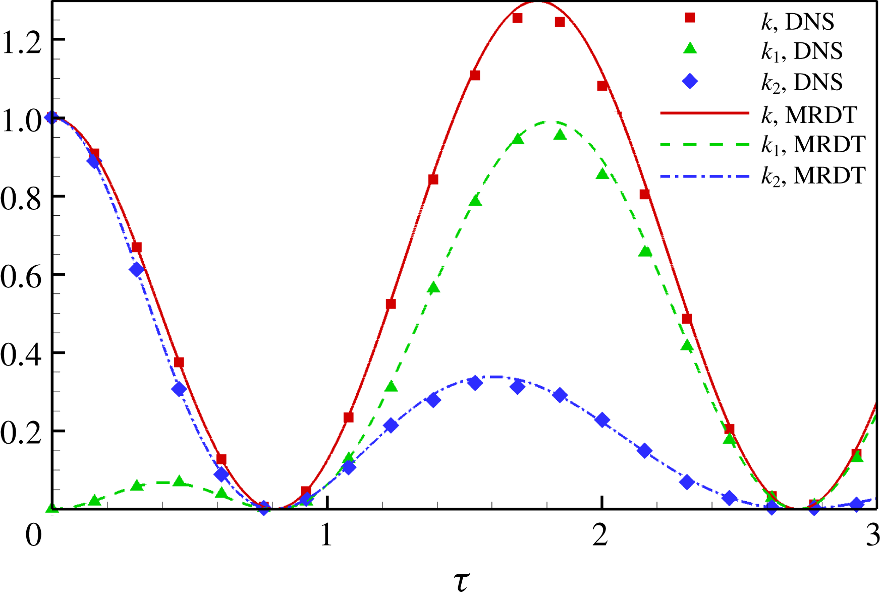
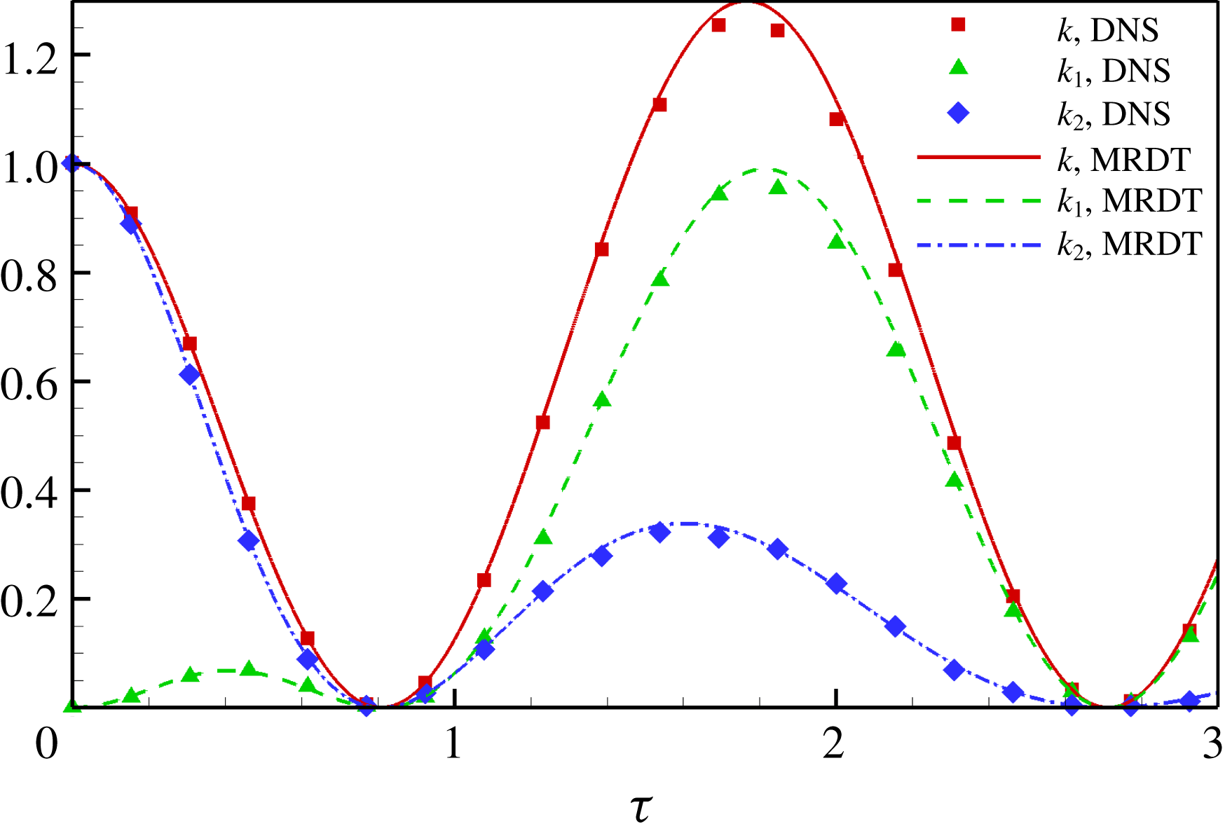
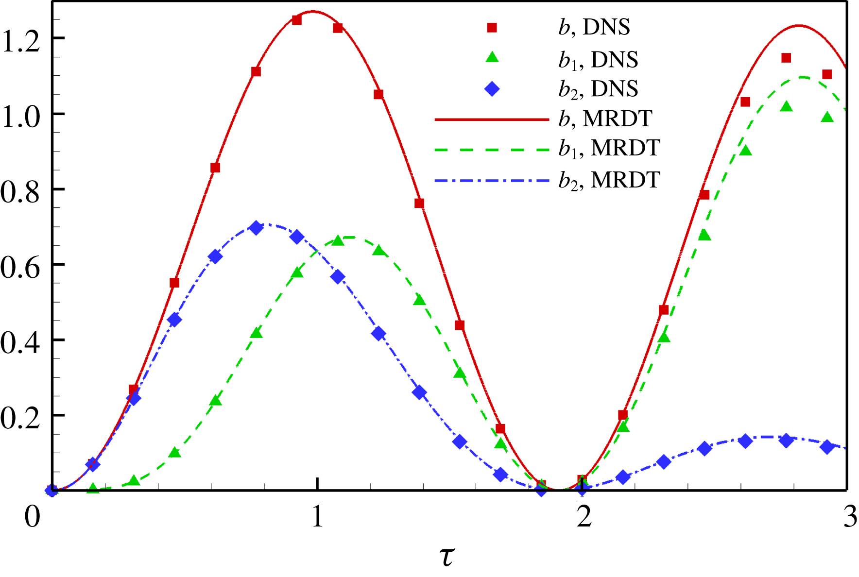
occur nearly simultaneously. The kinetic and magnetic energies for
 $R_{A}=1.7,$
 $\unicode[STIX]{x1D6FD}=0^{\circ }$
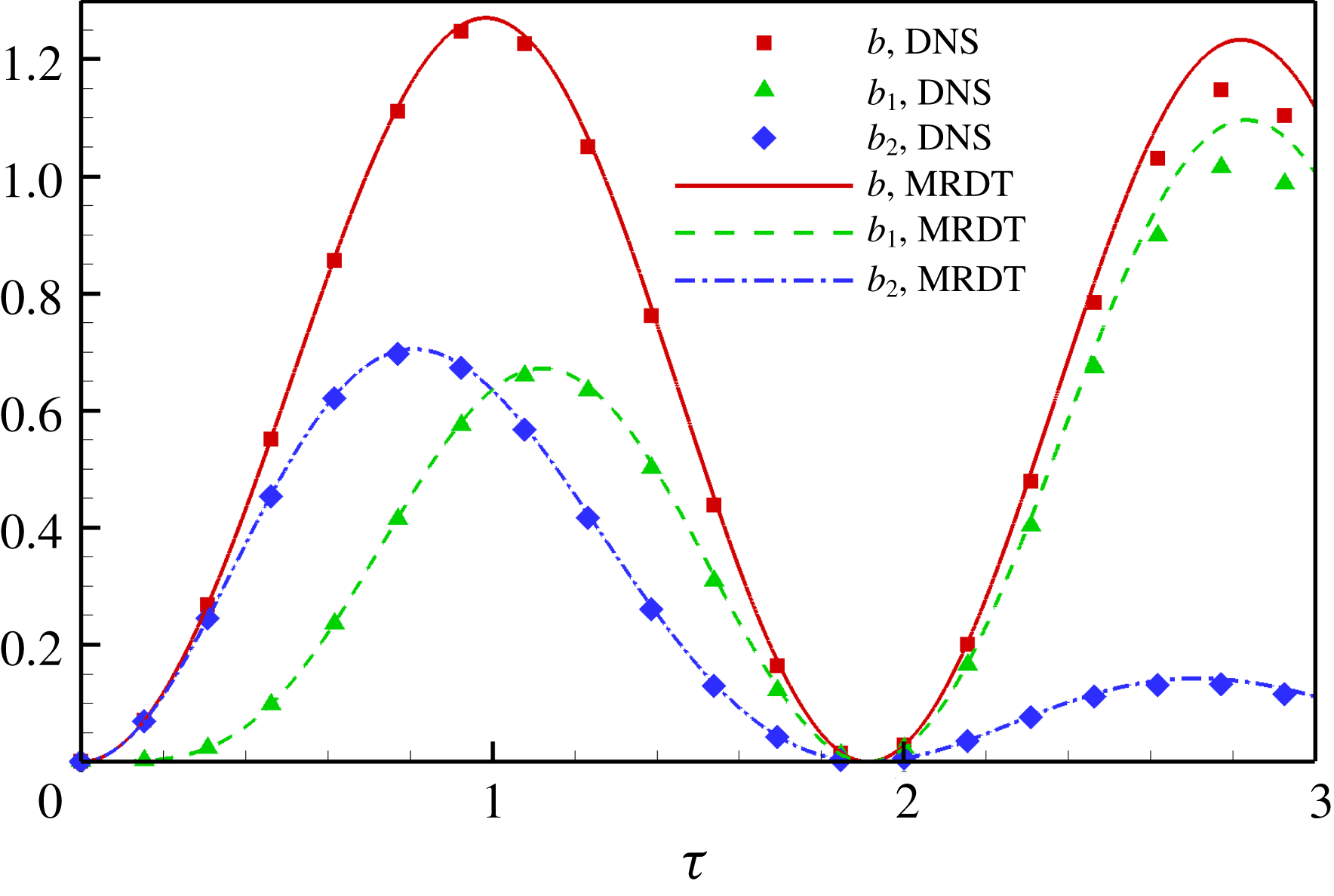
are presented in figures 13 and 14, respectively. During the course of evolution, the magnetic energy (
 $b$
) exceeds the initial perturbation kinetic energy (
 $k_{0}$
) owing to magnetic stretching. Here
 $k_{2}$
is transferred to
 $k_{1}$
owing to pressure redistribution. Even though the production of
 $k_{1}$
in this case is negative (
 $\unicode[STIX]{x1D6FD}=0^{\circ }$
), it has negligible influence on the evolution of
 $k$
owing to the oscillatory nature of
 $u_{2}^{\prime }$
seen from the beginning. The kinetic energy (
 $k$
) becomes zero at
 $\unicode[STIX]{x1D70F}\approx 0.75$
and then increases owing to harmonic exchange. An overshoot is seen in
 $k$
owing to harmonic exchange, at the end of first cycle of exchange. After this time, harmonic exchange prevails and the sum of kinetic and magnetic energy production goes to zero.
Intermediate
 $R_{A}$
regime (
 $R_{A}=1.7$
): evolution of kinetic energies (
 $k,k_{1},k_{2}$
) obtained using DNS and MRDT for
 $\unicode[STIX]{x1D6FD}=0^{\circ }$
.
Intermediate
 $R_{A}$
regime (
 $R_{A}=1.7$
): evolution of magnetic energies (
 $b,b_{1},b_{2}$
) obtained using DNS and MRDT for
 $\unicode[STIX]{x1D6FD}=0^{\circ }$
.
5.3 High magnetic field regime,
$R_{A}\gg 1$

In this regime, the magnetic field evolution is rapid enough that all the stages identified in
 $R_{A}\ll 1$
occur nearly simultaneously. As seen in § 3.1.2, in the linear limit of this
 $R_{A}$
regime, the evolution of
 $k_{2}$
and
 $b_{2}$
are given by
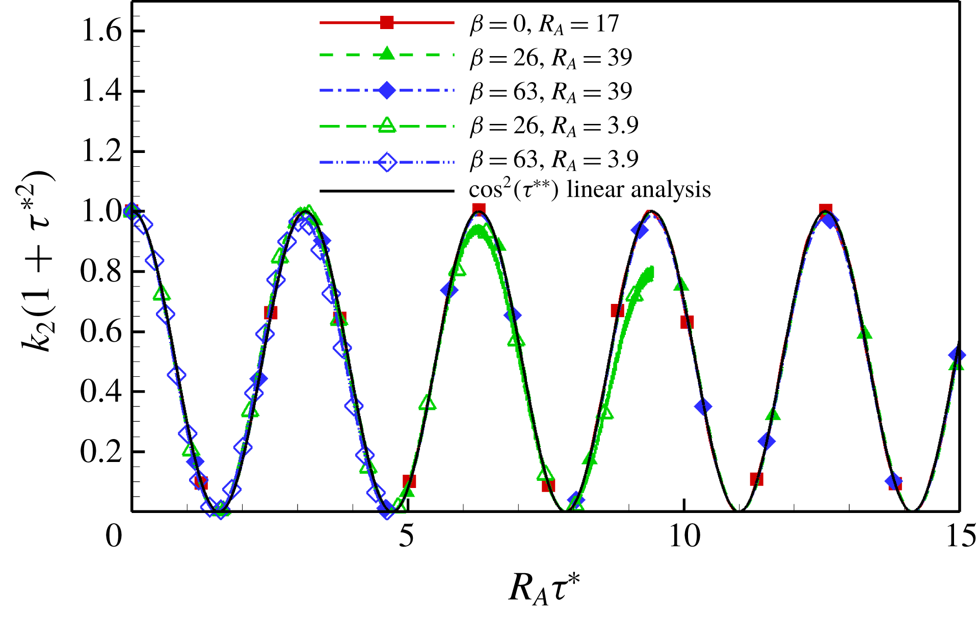
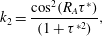 $$\begin{eqnarray}\displaystyle & \displaystyle k_{2}=\frac{\cos ^{2}(R_{A}\unicode[STIX]{x1D70F}^{\ast })}{(1+\unicode[STIX]{x1D70F}^{\ast 2})}, & \displaystyle\end{eqnarray}$$
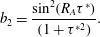 $$\begin{eqnarray}\displaystyle & \displaystyle b_{2}=\frac{\sin ^{2}(R_{A}\unicode[STIX]{x1D70F}^{\ast })}{(1+\unicode[STIX]{x1D70F}^{\ast 2})}. & \displaystyle\end{eqnarray}$$
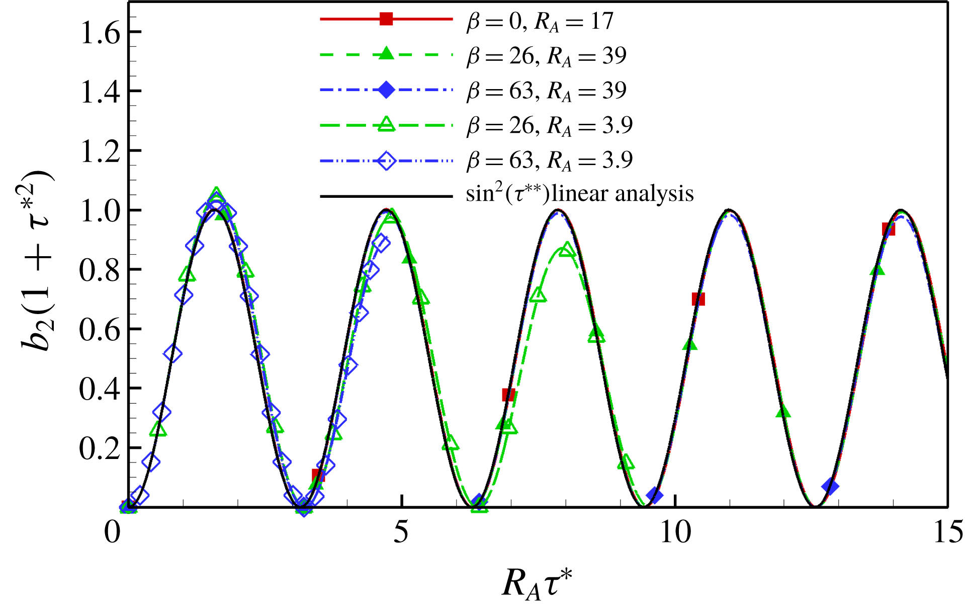
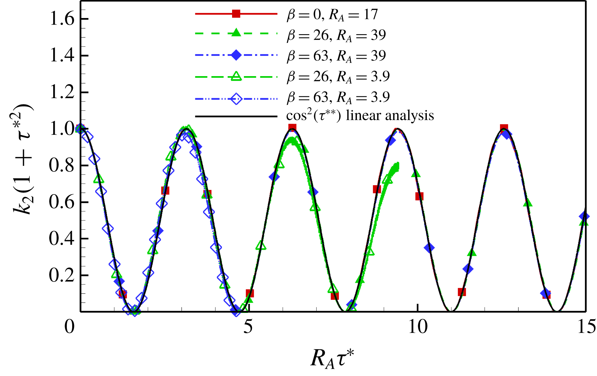
 $$\begin{eqnarray}\displaystyle & \displaystyle k_{2}(1+\unicode[STIX]{x1D70F}^{\ast 2})=\cos ^{2}(R_{A}\unicode[STIX]{x1D70F}^{\ast })=\cos ^{2}(\unicode[STIX]{x1D70F}^{\ast \ast }), & \displaystyle\end{eqnarray}$$
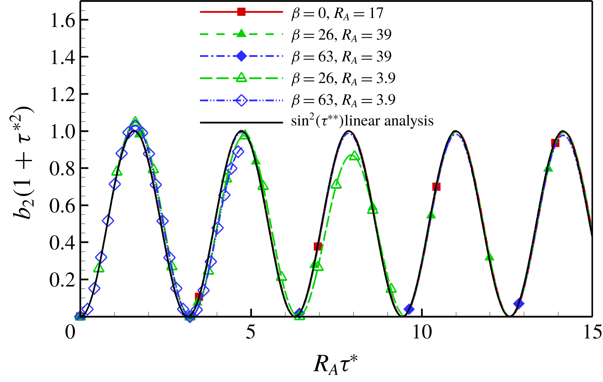
 $$\begin{eqnarray}\displaystyle & \displaystyle b_{2}(1+\unicode[STIX]{x1D70F}^{\ast 2})=\sin ^{2}(R_{A}\unicode[STIX]{x1D70F}^{\ast })=\sin ^{2}(\unicode[STIX]{x1D70F}^{\ast \ast }), & \displaystyle\end{eqnarray}$$
 $\unicode[STIX]{x1D70F}^{\ast \ast }=R_{A}\unicode[STIX]{x1D70F}^{\ast }$
. Using the above equations, the computed
 $k_{2}$
and
 $b_{2}$
in all cases with
 $R_{A}>2$
are plotted in the timescale
 $\unicode[STIX]{x1D70F}^{\ast \ast }$
. Figures 15 and 16 demonstrate the excellent agreement of the DNS results with linear theory and confirm the self-similar state of
 $k_{2}$
and
 $b_{2}$
in this
 $R_{A}$
regime.
High
 $R_{A}$
regime: evolution of
 $k_{2}$
obtained using DNS for
 $R_{A}=3.9,17,39$
;
 $\unicode[STIX]{x1D6FD}=0^{\circ },26^{\circ },63^{\circ }$
. The analytical solution of MRDT,
 $k_{2}(1+\unicode[STIX]{x1D70F}^{\ast 2})=\cos ^{2}(\unicode[STIX]{x1D70F}^{\ast \ast })$
, is also presented.
High
 $R_{A}$
regime: evolution of
 $b_{2}$
obtained using DNS for
 $R_{A}=3.9,17,39$
;
 $\unicode[STIX]{x1D6FD}=0^{\circ },26^{\circ },63^{\circ }$
. The analytical solution of MRDT,
 $b_{2}(1+\unicode[STIX]{x1D70F}^{\ast 2})=\sin ^{2}(\unicode[STIX]{x1D70F}^{\ast \ast })$
, is also presented.
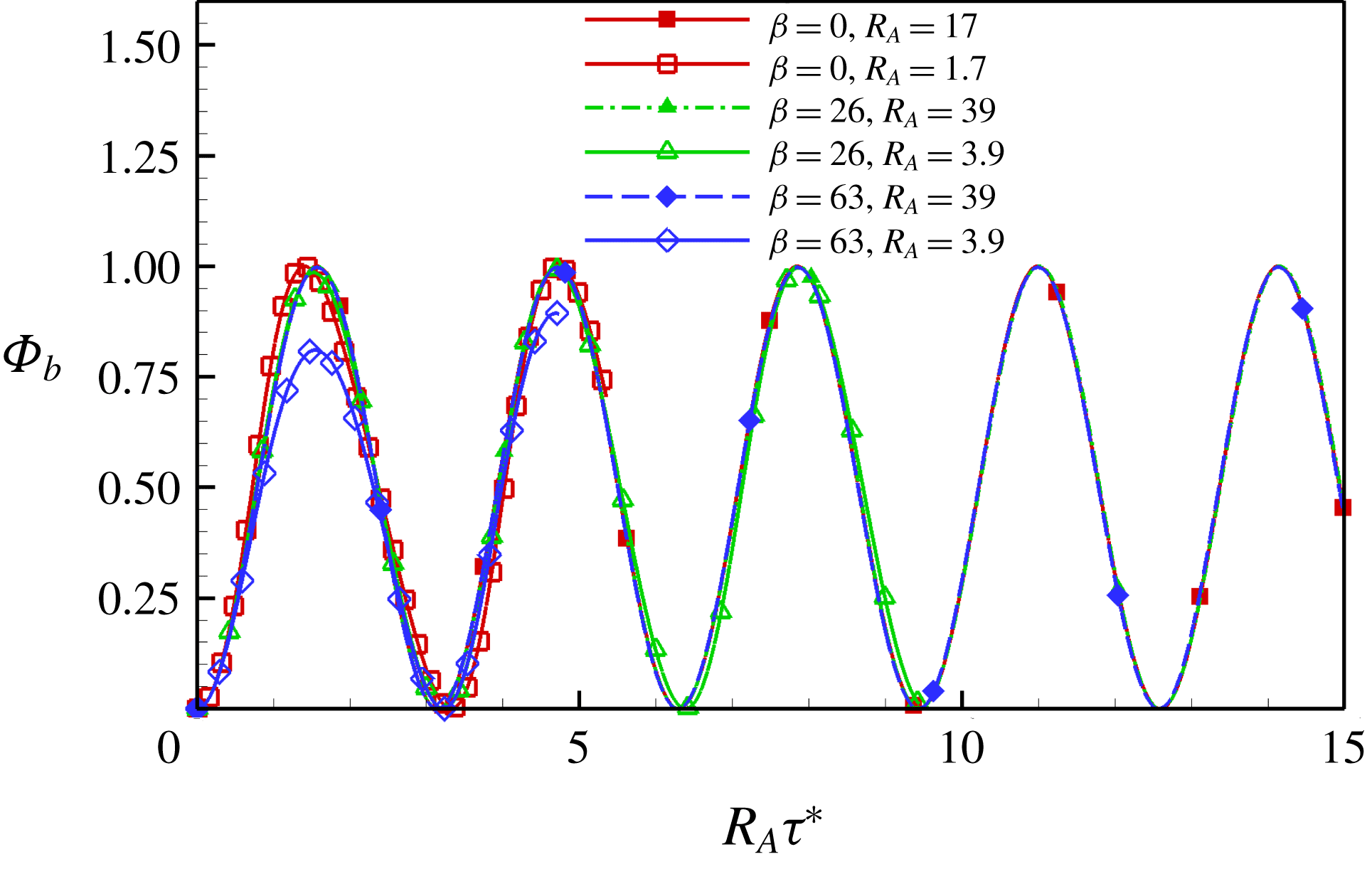
Linear analysis also suggests equipartition between perturbation kinetic and magnetic energies in the high
 $R_{A}$
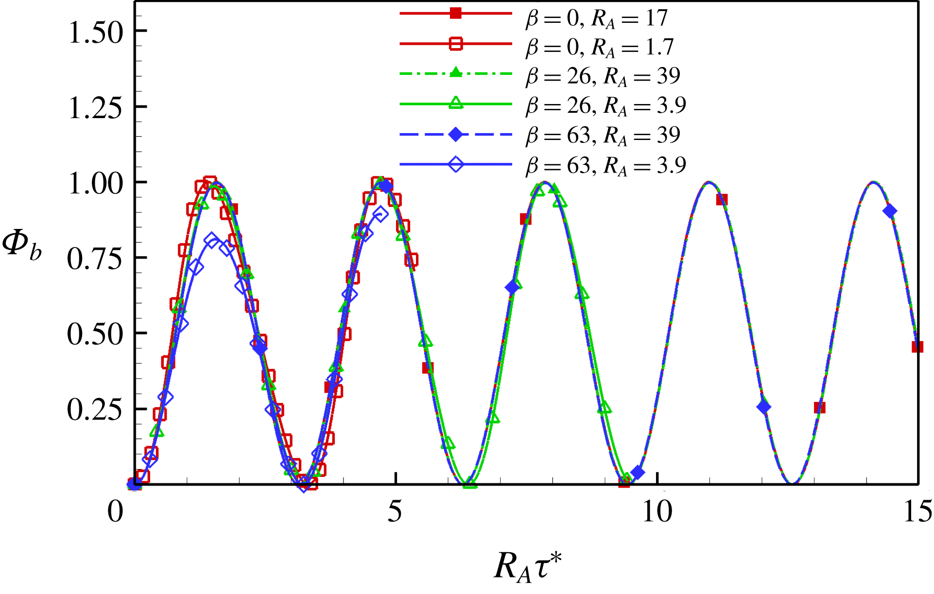
limit. To understand how the perturbation energies are distributed between magnetic and kinetic components, we define the energy partition function (
 $\unicode[STIX]{x1D6F7}_{b}$
) as follows:
 $$\begin{eqnarray}\unicode[STIX]{x1D6F7}_{b}=\frac{b}{k+b}.\end{eqnarray}$$
This definition is similar to that of Sarkar et al. (Reference Sarkar, Erlebacher, Hussaini and Kreiss1991) for dilatational kinetic and potential energies. Equipartition would imply that the energy partition function (
 $\unicode[STIX]{x1D6F7}_{b}$
) oscillates about 0.5. To verify this, we plot
 $\unicode[STIX]{x1D6F7}_{b}$
from DNS of intermediate and high
 $R_{A}$
cases (exchange dominates at all times) for all perturbation orientations,
 $\unicode[STIX]{x1D6FD}=0^{\circ },26^{\circ },63^{\circ }$
. A timescale of
 $R_{A}\unicode[STIX]{x1D70F}^{\ast }$
is chosen so as to demonstrate the self-similar behaviour at different
 $\unicode[STIX]{x1D6FD},R_{A}$
values. Figure 17 verifies that
 $\unicode[STIX]{x1D6F7}_{b}$
oscillates about 0.5 demonstrating equipartition of kinetic and magnetic energies. Another observation consistent with equipartition is that production and magnetic stretching are of comparable magnitudes and opposite in sign with a phase difference of
 $\unicode[STIX]{x03C0}/2$
. This leads to zero net growth of
 $k+b$
when integrated over a cycle.
Energy partition function (
 $\unicode[STIX]{x1D6F7}_{b}$
) obtained using DNS plotted for
 $R_{A}=1.7,3.9,17,39$
;
 $\unicode[STIX]{x1D6FD}=0^{\circ },26^{\circ },63^{\circ }$
.
As a result, pressure reorientation and exchange are the only significant processes in this regime. Investigating the sum of kinetic and magnetic energies, i.e.
 $(k+b)$
,
 $(k_{1}+b_{1})$
,
 $(k_{2}+b_{2})$
and
 $(k_{3}+b_{3})$
, removes the effect of harmonic exchange and highlights the effect of pressure redistribution at different
 $\unicode[STIX]{x1D6FD}$
:
 $$\begin{eqnarray}\displaystyle & \displaystyle \frac{\text{d}(k+b)}{\text{d}\unicode[STIX]{x1D70F}}=-2\text{Re}(\hat{u} _{2}\bar{\hat{u} }_{1})+2\text{Re}(\hat{B}_{2}\bar{\hat{B}}_{1}), & \displaystyle\end{eqnarray}$$
 $$\begin{eqnarray}\displaystyle & \displaystyle \frac{\text{d}(k_{1}+b_{1})}{\text{d}\unicode[STIX]{x1D70F}}=-2\text{Re}(\hat{u} _{2}\bar{\hat{u} }_{1})\left(1-\frac{2\cos ^{2}(\unicode[STIX]{x1D6FD})}{1+\cos ^{2}(\unicode[STIX]{x1D6FD})\unicode[STIX]{x1D70F}^{2}}\right)+2\text{Re}(\hat{B}_{2}\bar{\hat{B}}_{1}), & \displaystyle\end{eqnarray}$$
 $$\begin{eqnarray}\displaystyle & \displaystyle \frac{\text{d}(k_{2}+b_{2})}{\text{d}\unicode[STIX]{x1D70F}}=-2\text{Re}(\hat{u} _{2}\bar{\hat{u} }_{2})\frac{2\cos ^{2}(\unicode[STIX]{x1D6FD})\unicode[STIX]{x1D70F}}{1+\cos ^{2}(\unicode[STIX]{x1D6FD})\unicode[STIX]{x1D70F}^{2}}, & \displaystyle\end{eqnarray}$$
 $$\begin{eqnarray}\displaystyle & \displaystyle \frac{\text{d}(k_{3}+b_{3})}{\text{d}\unicode[STIX]{x1D70F}}=2\text{Re}(\hat{u} _{2}\bar{\hat{u} }_{3})\frac{2\cos (\unicode[STIX]{x1D6FD})\sin (\unicode[STIX]{x1D6FD})}{1+\cos ^{2}(\unicode[STIX]{x1D6FD})\unicode[STIX]{x1D70F}^{2}}. & \displaystyle\end{eqnarray}$$
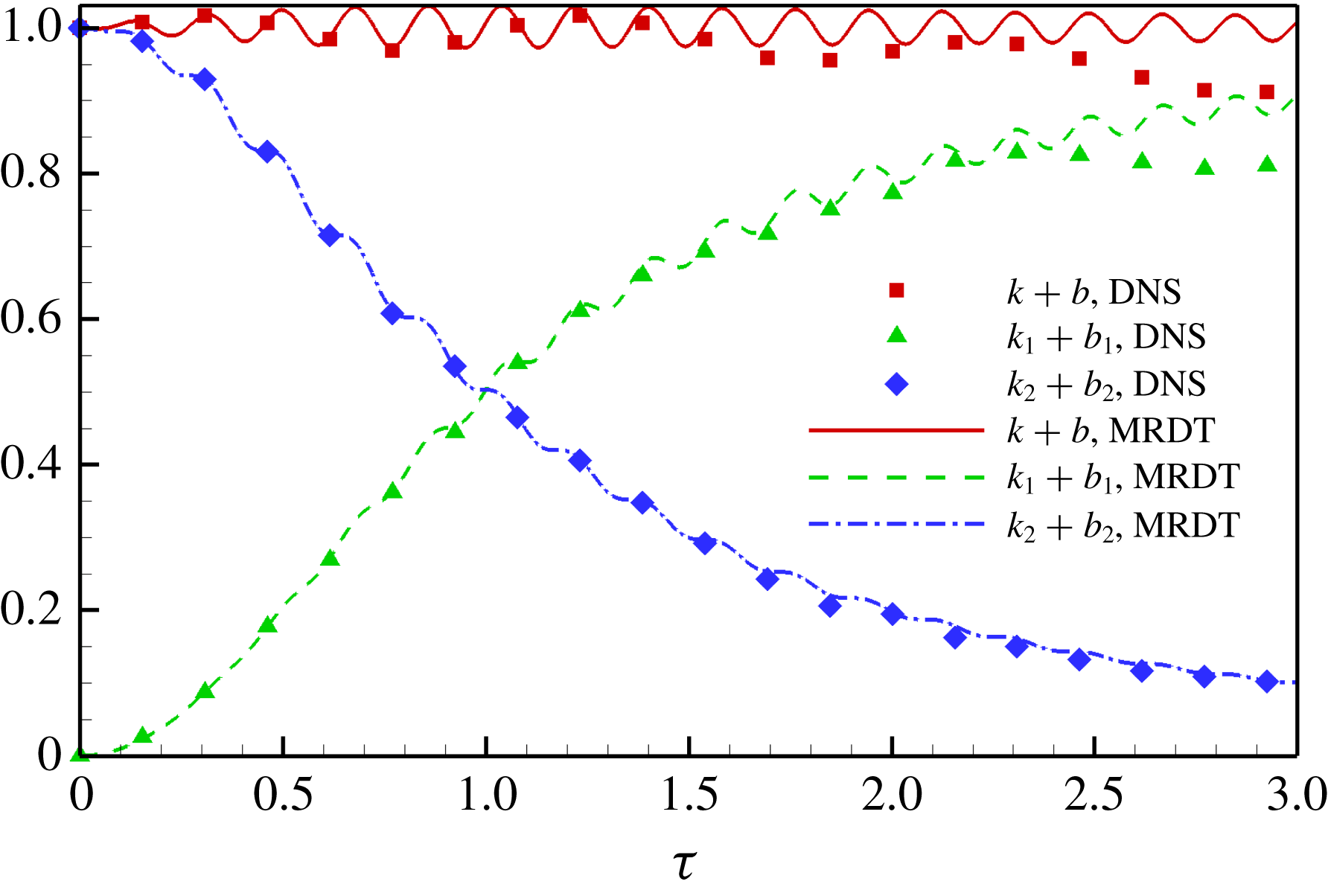
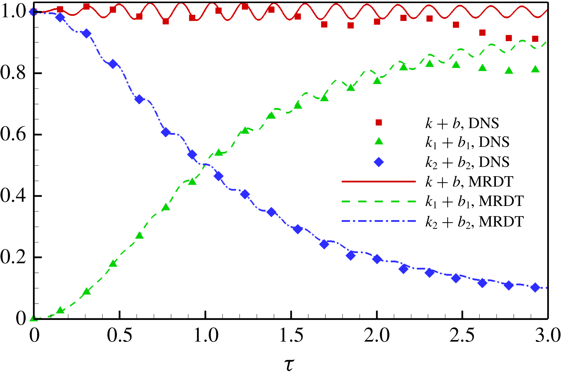
The case of
 $R_{A}=17,\unicode[STIX]{x1D6FD}=0^{\circ }$
is investigated first. It can be seen from figure 18 that the sum of kinetic and magnetic energies (
 $k+b$
) obtained from DNS remains nearly constant. For
 $\unicode[STIX]{x1D6FD}=0^{\circ }$
, production is always negative (3.35) and magnetic stretching is always positive (3.37). This implies that the sum of production and stretching becomes negligible owing to the rapid oscillatory nature of
 $u_{2}^{\prime }$
and
 $B_{2}^{\prime }$
with a phase difference of
 $\unicode[STIX]{x03C0}/2$
. Overall, energy transfer occurs from
 $(k_{2}+b_{2})$
to
 $(k_{1}+b_{1})$
owing to pressure redistribution. The slight decrease in the value of
 $(k+b)$
from unity is a result of the viscous and resistive effects included in DNS.
High
 $R_{A}$
regime (
 $R_{A}=17$
): evolution of the sum of kinetic and magnetic energies (
 $k+b,k_{1}+b_{1},k_{2}+b_{2}$
) obtained using DNS and MRDT for
 $\unicode[STIX]{x1D6FD}=0^{\circ }$
. Here
 $k_{3}+b_{3}$
is zero at all times.
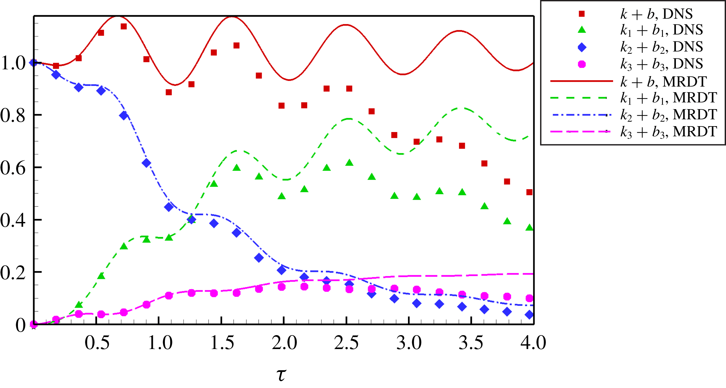
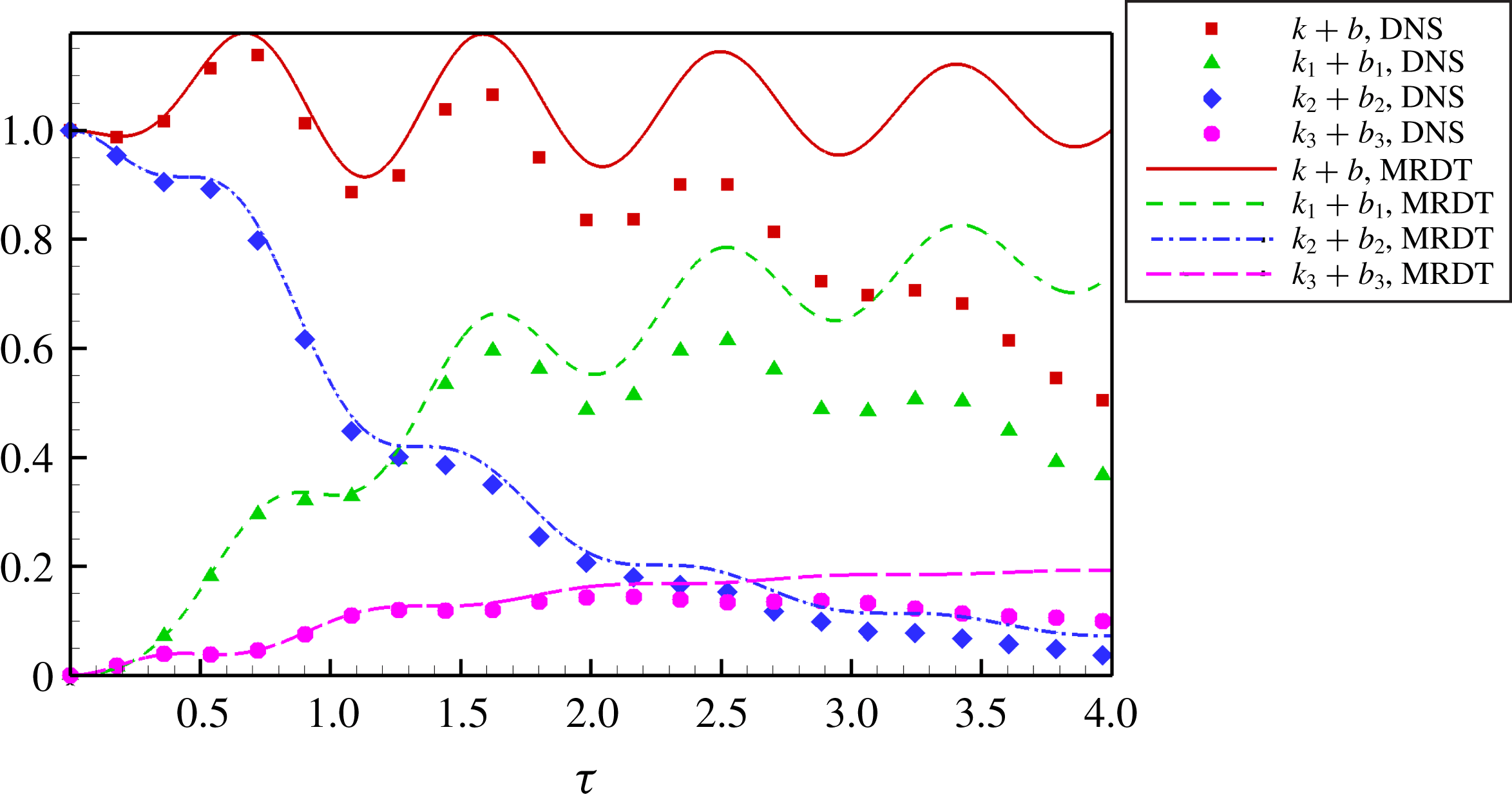
We now investigate the evolution of magnetic and kinetic perturbations for the case of
 $\unicode[STIX]{x1D6FD}=26^{\circ }$
,
 $R_{A}=3.9$
. From figure 19, it can be seen that the sum of kinetic and magnetic energies decays a little faster than
 $\unicode[STIX]{x1D6FD}=0^{\circ }$
,
 $R_{A}=17$
since the fluid and magnetic Reynolds numbers are lower. The frequency of oscillation of
 $u_{2}^{\prime },B_{2}^{\prime }$
is lower than that of
 $\unicode[STIX]{x1D6FD}=0^{\circ }$
case. As a result, the flow experiences longer periods of positive stretching and negative production. This results in larger-amplitude oscillations as compared with the
 $\unicode[STIX]{x1D6FD}=0^{\circ }$
case. Here
 $(k_{2}+b_{2})$
loses energy to
 $(k_{1}+b_{1})$
and
 $(k_{3}+b_{3})$
owing to pressure redistribution and
 $(k_{1}+b_{1})$
dominates at late times.
High
 $R_{A}$
regime (
 $R_{A}=3.9$
): evolution of the sum of kinetic and magnetic energies (
 $k+b,k_{1}+b_{1},k_{2}+b_{2},k_{3}+b_{3}$
) obtained using DNS and MRDT for
 $\unicode[STIX]{x1D6FD}=26^{\circ }$
.
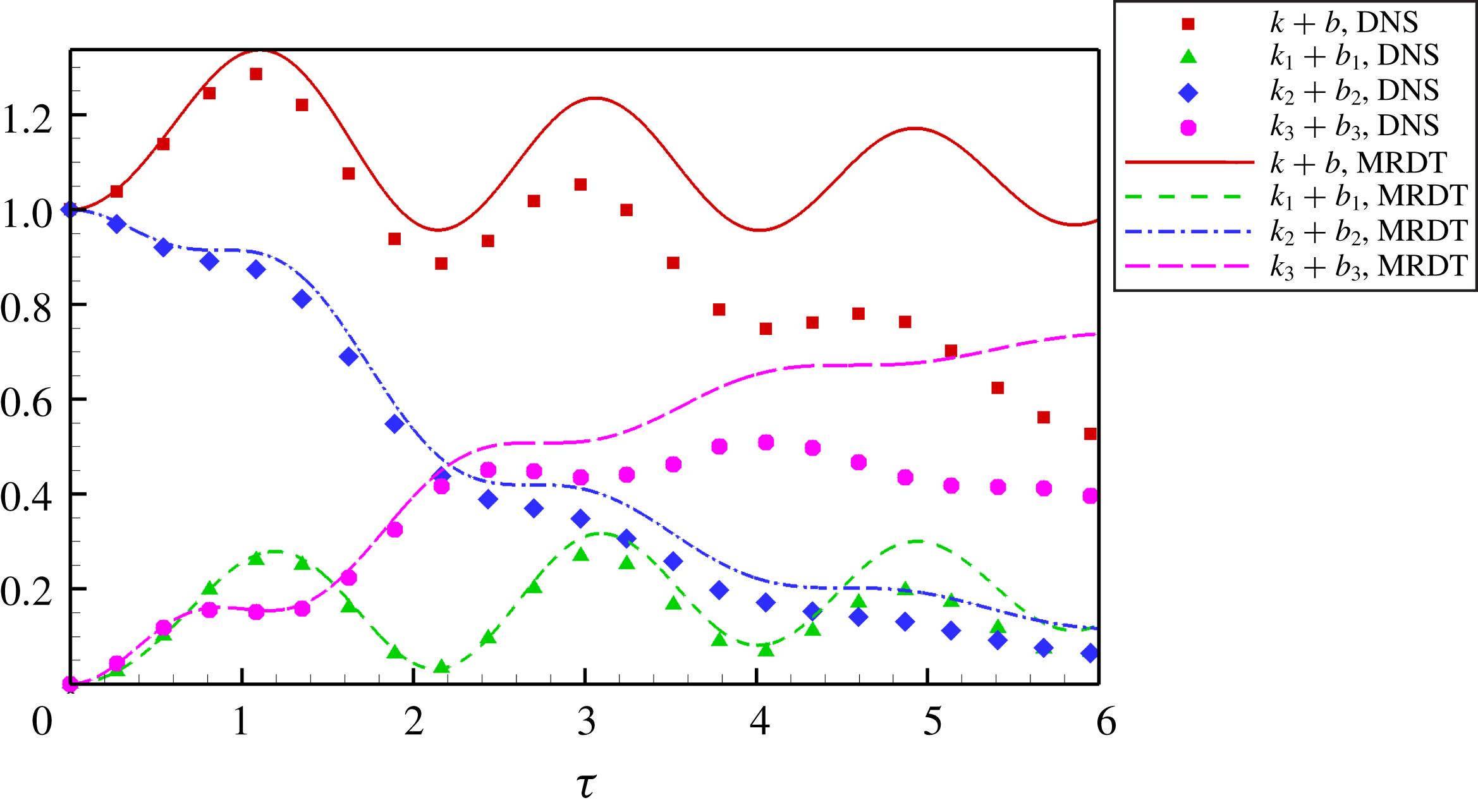
For
 $\unicode[STIX]{x1D6FD}=63^{\circ }$
,
 $R_{A}=3.9$
shown in figure 20, the timescale (
 $\unicode[STIX]{x1D70F}^{\ast }=\unicode[STIX]{x1D70F}\cos (\unicode[STIX]{x1D6FD})$
) at which exchange between magnetic and kinetic energies occurs is slower than that of the
 $\unicode[STIX]{x1D6FD}=26^{\circ }$
case. This, in addition to initial positive production and stretching, results in even larger-amplitude oscillations in
 $(k+b)$
compared with the
 $\unicode[STIX]{x1D6FD}=0^{\circ },26^{\circ }$
cases. At late times, however, production becomes negative and stretching becomes positive. Thus, the sum of production and stretching becomes negligible when integrated over a cycle. At early times,
 $(k_{2}+b_{2})$
loses energy to
 $(k_{3}+b_{3})$
and gains energy from
 $(k_{1}+b_{1})$
owing to redistribution and
 $(k_{3}+b_{3})$
dominates at late times.
High
 $R_{A}$
regime (
 $R_{A}=3.9$
): evolution of the sum of kinetic and magnetic energies (
 $k+b,k_{1}+b_{1},k_{2}+b_{2},k_{3}+b_{3}$
) obtained using DNS and MRDT for
 $\unicode[STIX]{x1D6FD}=63^{\circ }$
.
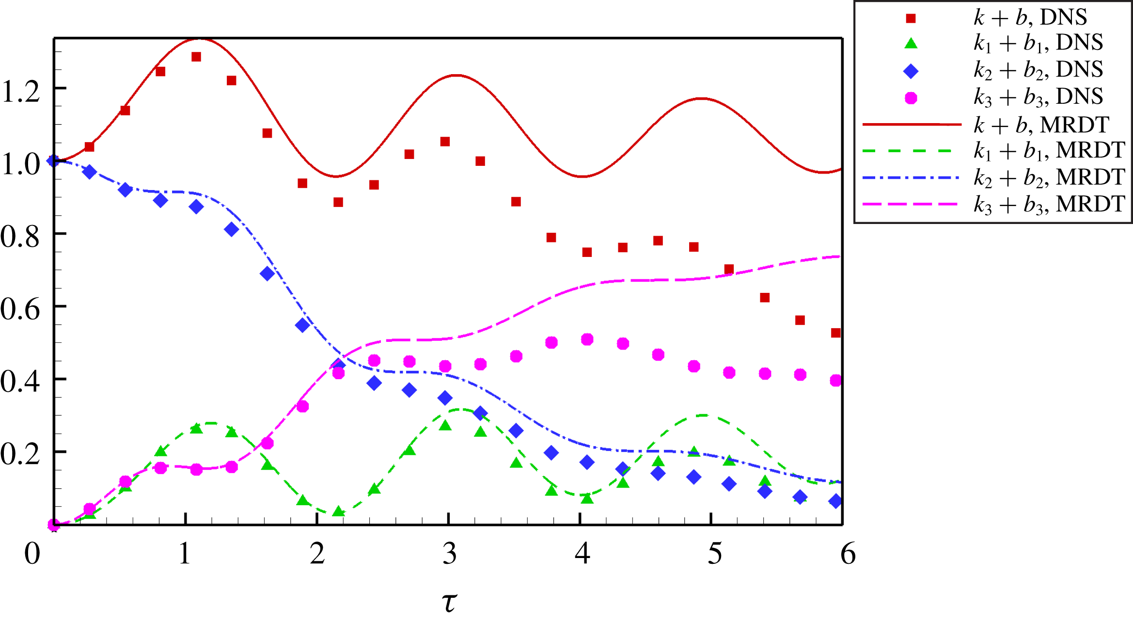
5.4 Viscous versus inviscid MRDT
We now compare the evolution of viscous MRDT with that of the inviscid limit. Figure 21 shows the evolution of kinetic energy (
 $k$
) for viscous and inviscid MRDT for
 $\unicode[STIX]{x1D6FD}=0^{\circ }$
at low and moderate
 $R_{A}$
values. Similar
 $Re,Re_{m}$
values as in the DNS calculations are chosen for viscous MRDT calculations. At low
 $R_{A}$
, comparing the behaviour of
 $k$
in the viscous limit, where
 $Re=Re_{m}=10^{5}$
, with that of the inviscid solution, we observe that the two calculations agree well with one another. This implies that for the time ranges investigated in the low
 $R_{A}$
regime, there is no considerable effect of viscous and resistive action on the perturbation evolution. For the moderate
 $R_{A}(=1.7)$
case where
 $Re=770$
and
 $Re_{m}=195$
, the viscous solution experiences a considerable amount of decay. However, for the times
 $\unicode[STIX]{x1D70F}<3$
presented in the DNS solution (figure 13), viscous and inviscid MRDT agree well with one another.
Viscous versus inviscid MRDT (
 $\unicode[STIX]{x1D6FD}=0^{\circ }$
): kinetic energy (
 $k$
) in the inviscid limit compared against viscous MRDT at low
 $R_{A}=0.39$
,
 $Re=Re_{m}=10^{5}$
and moderate
 $R_{A}=1.7$
,
 $Re=770$
,
 $Re_{m}=195$
.
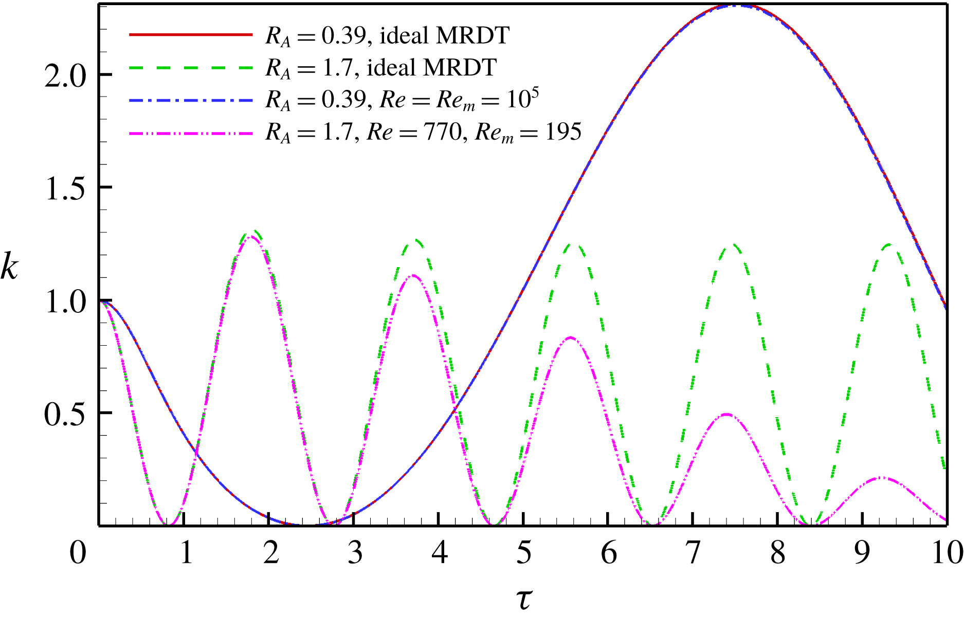
6 Summary and conclusions
The goal of this paper was to investigate the fundamental flow and flow–magnetic field interaction mechanisms that exert a stabilizing influence on perturbations in sheared MHD flows. Four constituent mechanisms have been identified: pressure redistribution, kinetic energy production, kinetic–magnetic harmonic exchange and magnetic stretching. Linear analysis and DNS are performed to characterize the role of different mechanisms in different parameter regimes of magnetic field strength (
 $B_{0}$
) and wavevector orientation (
 $\unicode[STIX]{x1D6FD}$
).
To establish the fundamental character of these mechanisms, velocity and magnetic field perturbations are investigated in homogeneously sheared MHD flows. Linear analysis identifies the ratio of shear and magnetic timescales,
 $R_{A}\equiv V_{A}\unicode[STIX]{x1D705}/S$
, as the parameter that characterizes the effect of relative timescales of magnetic and fluid processes. Velocity and magnetic field perturbations in the normal direction are identified as crucial, as they influence the production and magnetic stretching terms. For a given value of
 $R_{A}$
, these perturbations have identical evolution at all
 $\unicode[STIX]{x1D6FD}$
with respect to
 $\unicode[STIX]{x1D70F}^{\ast }=\unicode[STIX]{x1D70F}\cos \unicode[STIX]{x1D6FD}$
. This implies that as
 $\unicode[STIX]{x1D6FD}$
increases, the time elapse becomes slower. The primary findings of this paper are now summarized.
Spanwise perturbations. For this orientation, the velocity and magnetic field equations are decoupled. In addition the velocity evolution is impervious to pressure (pressure-released). This results in a quadratic growth of kinetic energy.
Low magnetic field regime for
 $\unicode[STIX]{x1D6FD}\in [\!0^{\circ },90^{\circ }\!)$
. In this limit, a three-stage perturbation evolution is seen. At initial times, the kinetic energy follows the hydrodynamic evolution. A slight transfer to magnetic perturbations is also seen in this stage. During the second stage, magnetic perturbations are amplified owing to magnetic stretching. At late times, harmonic exchange dominates. This results in equipartition of energy at late times.
Intermediate magnetic field regime for
 $\unicode[STIX]{x1D6FD}\in [\!0^{\circ },90^{\circ }\!)$
. For this shear-to-magnetic timescale ratio, the first and second stages seen in the low magnetic field regime occur simultaneously. As a result, magnetic stretching, production and pressure redistribution occur in the first stage. The second stage is characterized by harmonic kinetic–magnetic exchange. This again results in equipartition of kinetic and magnetic energies.
High magnetic field regime for
 $\unicode[STIX]{x1D6FD}\in [0^{\circ },90^{\circ })$
. In this limit, all three stages occur simultaneously. This results in negligible net production and magnetic stretching. Pressure redistribution and harmonic exchange are the only dominant processes. Equipartition is prevalent at all times owing to harmonic exchange.
This work is the first of a three-part study. The findings of this paper establish the fundamental nature of perturbation evolution in homogeneous shear flows at various values of shear-to-magnetic timescale ratios (
 $R_{A}$
). The second study extends the non-modal linear analysis to inhomogeneous shear flows, specifically mixing layers. For inhomogeneous shear flows the flow domain at a particular moment experiences various
 $R_{A}$
regimes owing to the inhomogeneity in shear. Since the transient behaviour of perturbations is understood for various
 $R_{A}$
values, the inferences from the current study will help establish the locations of stabilization of magnetic field in both linear and nonlinear stages of flow field evolution. This is unique to non-modal analysis as modal analysis would only indicate whether there is linear stabilization in the asymptotic limit. The final (third) study of this sequence involves comparing and contrasting the effects of compressibility and magnetic field on shear flow instabilities.
Acknowledgements
Portions of this research were conducted with the advanced computing resources provided by Texas A&M High Performance Research Computing.