


Introduction
Ice-core paleoclimate studies rely on stable-isotope ratios, particularly δ 18O, to provide continuous and detailed temperature records. The relationship between δ 18O and temperature T, for time t, is assumed to be linear

where a and b are coefficients that do not vary with time.
Even if Equation (1) is not strictly valid (Reference Jouzel and MerlivatJouzel and Merlivat, 1984), it is still important to ask what values of these coefficients are most appropriate since this relationship is in widespread use. There are two commonly used methods for finding values of these coefficients (Reference Robin and RobinRobin, 1983). The first is the spatial gradient method, which assumes that
where t0 is the present, ϕ and ω are latitude and longitude, and the coring site has location (ϕ0,ϕ0). One estimates the spatial relationship, δ18O(Τ(t0,ϕ,ω)), by measuring and correlating δ18O and temperature at a variety of locations. The slope and intercept of the correlation line provide estimates of α and b, respectively. Reference Peel, Mulvaney and DavisonPeel and others (1988) have shown that the assumption, Equation (2), is incorrect in one case. The second method is time-series analysis of histories of recent temperature and δ18O values. Time-series methods may give spurious results because detailed temperature records and isotope records are usually not available for the same location. Moreover, instrumental temperature records are necessarily of short duration and hence contain no information about low-frequency climate fluctuations.
The modern temperature-depth distribution in polar ice sheets is the result of the integrated response to past temperature and accumulation-rate changes. This makes possible a third method for calibrating the isotopic paleothermometer, if both a vertical temperature profile and an isotopic record are available for the same site; one can use a thermal model to determine values of a and b that generate a surface-temperature history which minimizes error between a solution of the model equations and a measured temperature profile (Reference Paterson and ClarkePaterson and Clarke, 1978).
Here, we present results of a borehole temperature-based calibration of the δ18O paleothermometer for the Greenland Ice Sheet Project II (GISP2) site in central Greenland and we argue that such calibrations are a useful tool for paleoclimatology. In addition, we present details of our thermal model and the inverse problem, examine the temporal range of applicability of our results, compare our results with modern spatial gradients of δ18O and temperature, and quantify the sensitivity of our results to model inputs for which the true value is not known. We allow three parameters to vary in our inversion: the two constant coefficients in Equation (1) and the initial surface temperature. Our inversion seeks to minimize the model mean-square-error, Ems , defined as
where Τ are modeled temperatures, θ are measured borehole temperatures and Ν is the number of grid points. We have already presented preliminary results in Cufley and others (1992).
Methods
We convert isotopic records into a history of ice-sheet surface temperatures using Equation (1). We then calculate a temperature-depth profile, using a forward numerical model forced with these surface temperatures. Comparison with measured borehole temperatures allows us to invert for best-fit values of a and b in Equation (1). This inversion is done for a 1340 year record of δ18O ending in AD 1989.
Measured temperatures
We use the temperature-depth profile measured by Reference Alley and KociAlley and Koci (1990) in a 217 m deep borehole at the GISP2 site near the summit of the Greenland ice sheet. Alley and Koci found the shape of the measured profile to be reproducible to ±0.01°C, although the absolute value of the temperatures was consistently ofiset by 0.035°C for two different factory-calibrated thermistors. Temperature gradients in the borehole are ≤0.04°Cm∡1, less than the adiabatic lapse-rate of air at these temperatures. In addition, the borehole is narrow, limiting the potential size of convection cells. Convective disturbance of the borehole-temperature profile is therefore unlikely (Reference DimentDiment, 1967). A repeat measurement of the borehole temperatures 1 year later by Alley and others confirmed that the trend was undisturbed. For both years, we observed that the thermistors’ resistance values were stable during measurement. Finally, the error resulting from distortion of the temperature distribution in the ice due to the presence of the air-filled borehole is insignificant for these low gradients (Reference SandersonSanderson, 1977). For all these reasons, we consider the borehole-temperature profile to reflect accurately the temperatures in the surrounding ice.
The model
Our thermal model is a one-dimensional finite-difference equation, similar to that used by Reference JohnsenJohnsen (1977), Reference Paterson and ClarkePaterson and Clarke (1978), Reference BolzanBolzan (1985) and Reference Alley and KociAlley and Koci (1990). Thermal energy per unit volume changes with time as (Reference MalvernMalvern, 1969, p. 228–30)
where ρ is ice/firn density, c is heat capacity, Τ is temperature, t is time, t
i and t
0 correspond respectively to the years AD 649 and AD 1989, z is depth (0 at the ice-sheet surface, increasing downward), k is thermal conductivity, w is vertical velocity, σ is the stress tensor, is the strain-rate tensor, and: indicates the inner product. is the rate of energy production due to non-mechanical sources. The first three terms on the righthand side of Equation (4) account for heat transfer by conduction and advection and heat generation due to mechanical work during strain. Values for heat capacity are taken from Reference YenYen (1981, p. 13, table 2). For thermal conductivity, we use empirical data for firn densities ρ 750 kgm−s (Reference YenYen, 1981, p. 16, equation 35). For ρ750 kg m−3, we use empirical k values for pure ice (Reference YenYen, 1981, p. 15, equation 33), and a theoretical extrapolation for dense firn (Reference YenYen, 1981, p. 17, equation 37).
The initial temperature, Ti(z), is a steady-state profile for an accumulation rate b = 0.24 m a−1 and surface temperature Ti(0). Equation (6) expresses Ti(0) as an offset, Δ, from the average temperature during the model run, T (a, b), which is a function of the coefficients in Equation (1). Note that Δ 0 indicates the average temperature over the last 1340 year was less than that during the preceding years. We have shown that Δ probably falls in the range 0.65–0.90°C, with a most probable value of 0.79°C (Reference Cuffey, Alley, Grootes and AnandakrishnanCuffey and others, 1992). This is similar to the result of Reference Dahl-Jensen and JohnsenDahl-Jensen and Johnsen (1986), suggesting a Medieval Warm Period of this magnitude at Dye 3. Because the shape of the steady-state profile is fixed, Teoo is uniquely determined by Ti(0) (Equation (7)).
The remaining terms in Equation (4) are given by:

Here, σz
is vertical stress and σx
is horizontal stress normal to the ice divide (i.e. east—west) and is the horizontal longitudinal strain rate in this direction. We partition the vertical longitudinal strain rate into components due to firn densification, and flow divergence, . We assume plane strain in vertical planes normal to the ice divide, so no terms appear for the north-south horizontal direction. Because our model includes only the top 20% of the ice thickness and because GISP2 is only 30 km west of the ice divide, we neglect the work terms involving shear deformation, which are orders of magnitude less at these depths and low surface slopes. Note that the product in Equation (9) gives the rate of heat dissipation due to work done moving grains closer together in the densification process, while the sum of the other two terms in Equation (9) gives the rate of heat dissipation due to the flow-divergence strain.
Incomprcssibility requires that the strain rates due to flow divergence sum to zero (Equation (10)). We assume that has a constant value equal to the mean annual ice-equivalent accumulation rate, b, divided by the ice-equivalent thickness, hi = 3100m (Reference Hodge, Wright, Bradley, Jacobel, Skou and VaughnHodge and others, 1990). We also assume power-law flow (n = 3) to write in terms of the vertical longitudinal deviatoric stress, σd
, and the usual flow-law pre-factor, A, taken from Reference PatersonPaterson (1981, p. 39) for a temperature of-30°C.
In Equation (11), wc write the vertical strain rate due to firn densification in terms of the material derivative of density (Dρ/Dt) and assume that the density at a given depth docs not change through time. Equation (12) expresses the balance of forces; the vertical normal stress equals the weight of overburden and the sum of the longitudinal deviatoric stresses vanishes. The vertical velocity equals the snowfall rate at the surface and decreases with depth as the integral of the vertical strain rate (Equation (13)).
Finally, we assume that thermal energy released by non-mechanical sources is negligible (Equation (14)). At locations with frequent surface melt, the latent heat released upon refreezing of meltwater at depth can dominate the temperature structure (Reference Paterson and ClarkePaterson and Clarke, 1978). The paucity of inferred melt layers in the GISP2 ice cores (Reference Alley, Grootes, Meese, Gow, Taylor and CuffeyAlley and others, 1991) indicates we can neglect this term. Another source of thermal energy is the elimination of surface area during ice-grain growth We neglect this term, too, based on the following argument. The surface area of grain boundaries per volume of ice, Agrains
, is approximately half the area of each grain (because each surface is largely shared by neighbouring grains) times the number of grains per volume. For spherical grains of radius r, A
grains ≈ 1.5/r.The rate of energy release is the product of surface energy associated with the ice—ice boundaries (γi
= 0.065 J m-2;, Reference HobbsHobbs, 1974, p. 440) and rate of elimination of grain-boundary area, or, for a steady distribution of grain-size with depth,
will be a maximum for shallow ice, where r ≈ 10-3 m, and r increases by approximately 1 mm per hundred meters, giving a temperature change at a rate (∂T/∂t) , which is more than
an order of magnitude less than strain heating (see below and Fig. 1).
Contribution of different heat-transfer and generation mechanisms to rate of temperature change (Ka−1) in the ice sheet, calculated for AD 1989. Absolute values for temperature-change rate were taken to make possible the logarithmic scale. This causes the sharp downward points where the sign of temperature change switches. We omit the lower 200 m to facilitate the view of the more interesting upper section.

Our model extends from the ice-sheet surface to 600 m depth, with uniform 6 m node spacing. Time step is 1 x 10⁶s (11.6 d). The density profile is measured and assumed constant, which is a reasonable assumption because long-term averages of temperature and accumulation rate do not vary significantly in the Holocene. Conductive-and advective-heat transport dominate the model, with heat generation due to densification playing a significant role in the 20–150 m depth range (see Fig. 1).
Forcings
Through time, the model is forced with surface temperatures, Ts , calculated from isotopic ratios (Equation (8)) and accumulation rates, b(t) calculated from seasonal indicators in the ice core (Reference Meese, Gow, Alley, Taylor and RamMeese and others, 1992) (see Fig. 2a and b).The age scale is accurate to a year or two for the most recent times and to a few per cent for older times (Reference Meese, Gow, Alley, Taylor and RamMeese and others, 1992). The isotopic ratios are measured using mass spectrometry. The uncertainty in a single δ 18O value is less than 0.1‰. We measured ten samples per year of ice and interpolated between these to get our temperature forcing. Mean annual δ 18O values have an analytic uncertainty of less than 0.03‰. Note that, if our δ measurements are systematically offset from true values, the intercept (b) value in Equation (1) will be offset by the same amount in our calibration.
The isotope and accumulation-rate data used in our calibration, smoothed using 10 year running average.
Inversion
Comparison of model equation solutions with measured borehole-temperature data enables us to invert for optimal values of the coefficients a and b Δ is also treated as a free parameter in the inversion. We use a multi-dimensional form of Newton’s method (Reference MenkeMenke, 1984) to find values of model parameters that give best agreement between model and measured temperatures, as defined by Equation (3). The inversion uses model grid points only from 36 to 216m depth, the bottom of the measured temperature record. The top 30 m are truncated to avoid extreme sensitivity of the calibration to the most recent several years. This is desirable because the natural variability of mean annual δ 18O values is large; because the shallowest part of our borehole may be affected by surface winds; and because the amplitude of shallow temperature variations is huge compared to those at greater depths.
An initial guess at values for the model parameters, mq
0 = [a, b, Δ], is changed by an amount , calculated from
where p = 1,... Ν and q = 1,... Μ (Ν = number of grid points = 31, M = number of free-model parameters≤3). Here is the temperature residual, Tp
(mq
0) - ϴp
, and Hpq
is a matrix of the derivatives of Tp
with respect to each model parameter, calculated numerically as
which we invert using singular-value decomposition to solve Equation (16). The new values are then modified in the same fashion with decreasing until E
ms ceases to decrease. The inversion to solve Equation (16) is overdetermined. We neglect no eigenvalues and we find that the model resolution matrix is approximately equal to the identity matrix, with off-diagonal elements smaller than 10−9.
We interpolate measured temperatures to each grid point, because the measured values have 5 m or less spacing, versus 6 m spacing for grid points. Because temperature varies gradually, this interpolation introduces insignificant error. Inversions of synthetic borehole temperatures produced by known values of a, b and Δ indicate that the numerical error of our technique is approximately ±0.001‰°C−1 for b, ±0.05‰ for b and ±0.005°C for Δ. In addition, the solutions do not change with variations in initial mq0 or with reasonable changes in the size of . We therefore consider our solutions to be accurate numerically.
In this paper, we map the error Ems as a surface over the a-b plane. The low point of this surface, which has error Ems min overlies the optimal values of the coefficients a a and b, a* and b*. This minimum is found by using mq = [a, b, Δ] in the inversion. Then we assign fixed values to a and use only mq = [6, Δ]. This defines a trough in the error surface that gives the best possible error for given a. It is important to define this trough because a is the parameter in our inversion of most interest to paleoclimate studies, since it relates the magnitude of variations in δ 18O to variations in temperature. Finally, we assign fixed values to both a and b, let mq = Δ, find the minimum Ems for these (a, b) coordinates and contour the resulting surface. This surface shows how confident we can be in our calibration. If the optimal values, a* and b*, are well-constrained, the error surface will rise rapidly along trajectories away from the coordinate (a*, b*). For us to claim that (a*, b*) makes a significantly better paleothermometer than (a, b) at a given level of statistical confidence, the ratio Ems(a, b)/Ems min should exceed the maximum ratio of squared errors expected from random fluctuations in the data alone, which is given by the F-distribution (see Reference MenkeMenke, 1984, p. 96–97). Thus we use an F-test that compares the surface Ems(a, b)/Ems min to outline regions in the a-b plane that contain the values of the true paleothermometer at various confidence levels. For optimal values of Δ, see Reference Cuffey, Alley, Grootes and AnandakrishnanCuffey and others (1992).
Time-weighting of the calibration
If the slope and intercept of the isotope-temperature relation (Equation (1)) have changed over time, then a and b from our calibration are time-averaged values for the most recent 1340 years. Furthermore, these are weighted averages, with some times contributing more than others. For example, very recent times are weighted lightly in the calibration because we disregard the uppermost part of the borehole-temperature profile where the effects of recent temperature change are largest. We calculate the weight function, W(τ), as a semi-quantitative measure of the influence of events in each of the 1340 years on the modern borehole-temperature profile; W(τ) therefore approximates the time-weighting of a and b in our calibration.
The surface-temperature history given by Equation (1) from the 1340 year δ 18O record is simplified to a series of annual average perturbations about the mean, δΤav(τ), for the rth year before present. In the modern ice sheet, each δΤav(τ), will have a temperature response at depth z
Here, is the temperature perturbation as a function of elapsed time that results from a unit forcing (1°C for 1 year) at time  . These are Green’s functions, which we compute numerically. Note that, because τ is given as years before present, τ equals .
The modern temperature at depth z depends on the sum over all years of the responses Rz(τ). Comparing the magnitude of Rz(τ) for different years τ therefore gives a measure of how important each year is for determining the modern temperature structure, compared to other years, at that depth. To present this comparison graphically, incorporating all depths used in the calibration, we define the depth-averaged weight function W(T), as
, where z(p) is the depth of the pth grid point used in the calibration.
We normalize W(τ) by setting the integral of W(τ) over the entire range 0 < τ < 1340 years equal to unity. Then gives the relative contribution of the interval τ1 < τ < τ2
to the modern temperature structure and hence to the calibration of the isotopic paleothermometer.
Modern local spatial gradient of δ 18O with temperature
One purpose of our paper is to argue that calibrating isotopic paleothermometers using borehole temperatures is a profitable undertaking. To this end, it is useful to compare results of our borehole calibration with results of the most frequently used calibration method, that based on spatial gradients (as defined in the Introduction).
We calculate a spatial gradient using data from locations within 100 km of the GISP2 site. One of us (unpublished manuscript by J. Bolzan) has measured 10 m temperatures in the GISP2 area and collected a number of shallow cores that span approximately 2545 years, and oxygen-isotope profiles were measured on these cores by the Geophysical Laboratory in Copenhagen (Reference Bolzan and StrobelBolzan and Strobel, 1994). Unfortunately, for logistical reasons, the isotope and temperature measurements were not made at the same sites. As a result, we interpolated the temperature field using a generalized Kriging algorithm (Reference OleaOlea, 1974) to generate mean annual temperatures at the shallow coring sites, except for two sites which we considered too distant from the nearest measured 10 m temperature. We then regressed isotopic values averaged over the most recent 30 year interval in the shallow cores against the interpolated mean annual temperatures. The one core that spanned only 25 years was not used.
Reference Clausen, Gundestrup, Johnsen, Bindschadler and ZwallyClausen and others (1988) measured 10 m borehole temperatures and δ 18O of ice cores south and east of the GISP2 site. We include these data in our correlation to widen the temperature range and increase the sample size. The isotopic data of Reference Clausen, Gundestrup, Johnsen, Bindschadler and ZwallyClausen and others (1988, fig. 4) are 30 year averages; we use the most recent value for each core. We do not use the data for Crête, because this core was drilled almost a decade before the others and therefore does not include the late 1970s and early 1980s in the 30 year average.
Results
By using the calibrated values, a* and b*, in Equation (8), our thermal model generates a temperature-depth profile that closely replicates the measured borehole temperatures (Fig. 3). The error surface, E ms(a,b), is a clearly defined narrow trough with a single minimum at (a* = 0.5305, b* = –18.18) (Fig. 4). Here, E ms(a*, b*) = E ms min = 6.58 × 10−. The long axis of the trough, which follows the line
is the direction along which the optimal values a* and b* are least well constrained (i.e. the trough follows an eigenvector of Hij ). The confidence intervals (Fig. 3), which are bounded by contours on the error surface, are roughly elliptical with the major axis much greater than the minor axis, indicating that, for a given a value, the b value is tightly constrained. The 90 and 95% confidence intervals on aare (0.453, 0.656) and (0.443, 0.689), respectively.
Comparison of model and measured temperatures. Model results are shown for the best-fit value a = 0.53, and for the values a = 0.45 and a = 0.70, which approximately bound the 95% confidence intervalfor a. The b values for these calculations are given by Equation (20).

Model mean-square-error surface, showing contours of 90, 99 and 99.9% confidence levels, and the best-fit value (asterisk). The intercept, b, is so closely constrainedfor given slope, a, that the contours appear as a line in the a-b plot in the upper panel,following Equation (20). The distance, db, of a contour from this line for given a is plotted in the lower panel.
The weight function for the GISP2 δ 18O paleothermometer attains its peak value at 58 years BP and decays rapidly backward in time (Fig. 5) to one-third of the peak value at 300 year BP and to near zero at 1200 year BP. Our calibration is most sensitive to temperature changes of the early to mid 20th century. The median of W(τ) is the year τ = 259 year BP (AD 1730). Hence, the calibration is as much determined by temperature changes occurring prior to 259 year BP as by more recent changes. Our calibration is therefore applicable to at least five or six centuries of δ 18O data.
The depth-averaged weight function. W(τ) for the GISP2 δ 18O paleothermometer. The area under the curve for a given time interval indicates the sensitivity of the modern temperature structure and the calibration to that interval. W(τ = 0) = 0, because we did not use the top 30 m of the borehole in the calibration.
The Bolzan data alone do not show a local spatial δ-Τ gradient (Fig. 6). Including the Reference Clausen, Gundestrup, Johnsen, Bindschadler and ZwallyClausen and others (1988) data still shows no clearly defined δ-Τ gradient but, for comparison with Equation (1), linear regression gives a = 0.47 and b =-20.1. The 95% confidence interval for o is (0.17,0.76) which is a large uncertainty compared to the uncertainty in the borehole-temperature calibration. Improving the spatial estimate would require drilling and analyzing more shallow cores.
The modern spatial gradient of δ and temperature from locations within 100 km of the GISP2 site, showing the Bolzan data and the Reference Clausen, Gundestrup, Johnsen, Bindschadler and ZwallyClausen and others (1988) data. There is no obvious relationship but we show the best linear fit (δ = 0.47T – 20.1) for comparison with Equation (1).
Sensitivity Tests
Methodology for the sensitivity tests
The values we use for the borehole temperatures and for some fixed parameters in our model may differ from the true values. It is important to know how this uncertainty may affect our calibration. Therefore, we test the sensitivity of the optimal values, a* and b*, to these uncertain model variables. We alter each model variationsable in question, V, by an amount or replace it by an alternative variable, Valt
, and repeat the inversion (mq
0 = [a,b,Δ]) using or Valt
. If the result has E
ms that is statistically significantly worse than E
ms
min, then the altered value is probably physically unreasonable. Otherwise, the inversion gives new, acceptable values for a* and b*.
We examine the sensitivity of the calibration to:
-
1. The basal boundary condition. We replace the constant basal temperature T600 , with a constant basal heat (lux implied by the steady-state initial temperature profile.
-
2. The initial temperature profile. In Equation (5), we replace the steady-state, nearly isothermal, profile with linear profiles
 where T
i is the temperature difference between the 600 m depth and the surface. It is unlikely that because there was a cooling trend during the late Holocene (Reference LambLamb, 1982; Reference Dahl-Jensen and JohnsenDahl-Jensen and Johnsen, 1986). It is also probable that is less than 1°C because the difference in mean annual temperature between the climatic optimum and the first millennium AD is at most several °C (Reference LambLamb, 1982; Reference Dahl-Jensen and JohnsenDahl-Jensen and Johnsen, 1986). The magnitude of the corresponding temperature maximum at depth will be considerably reduced by diffusion and the maximum will be deeper than 600 m due to advection alone. Therefore, we use and-1.0°C as estimates of this uncertainty.
-
3. The thermal properties of snow. For snow of density ρ < 750 kg m-3, we increase and decrease the dependence of thermal conductivity on density and temperature by the maximum amount that still approximates the data trends in figures 16 and 17 of Reference YenYen (1981). We alter the constants in Yen’s equation (35), so that thermal conductivity is 0.048 exp(0.0103T + 5.9289 ρ) for the increased dependence case; for the decreased dependence case it is 0.100 exp(0.0073T + 4.1456ρ) (units as in Reference YenYen (1981)).
-
4. The ice-equivalent thickness, hi The thickness of ice beneath Summit is uncertain by 100 m or more because of the uncertainties in velocity of radar waves through ice and the moderately coarse grid for radar surveys relative to the rough bedrock topography (Reference Hodge, Wright, Bradley, Jacobel, Skou and VaughnHodge and others, 1990). We have used hi = 3150m (Reference Hodge, Wright, Bradley, Jacobel, Skou and VaughnHodge and others, 1990). Here, we use
with . -
5. The borehole-temperature measurements.
 is less than 1°C because the difference in mean annual temperature between the climatic optimum and the first millennium AD is at most several °C (
The absolute value
The thermistors we used are accurate to better than ±0.1°C (Reference Alley and KociAlley and Koci, 1990). For these sensitivity tests, we shift the entire temperature profile by  ±0.1, 0.04 and 0.02°C.
The shape
The shape of the temperature profile was reproducible to 0.01°C. Therefore, the random error of each temperature measurement about its true value is probably less than 0.01°C in magnitude. We examine the statistically very unlikely worst-case scenario in which this error is systematically distributed such that the variation of the measured temperatures relative to their mean changes by an amount . We smoothly deform the measured temperature profile so that its mean value is unchanged but so that the maximum difference between measured temperature and mean measured temperature changes by
Results of the sensitivity tests
Results of the sensitivity tests show that realistic uncertainties in measured temperatures and model variables do not significantly affect our calibration (see Table 1). a* is insensitive to the basal boundary condition, the ice thickness and the absolute value of the measured borehole temperatures. It is weakly dependent on the initial temperature profile and on snow thermal properties, and more strongly dependent on systematic errors in the measured borehole-temperature trend. Because the temperature trend was highly reproducible using different measuring devices, we consider such systematic errors to be very unlikely. Assuming no such systematic error, the summed uncertainty in a* ranges from +0.040 (which obtains if ) to-0.038 (which obtains if , snow-thermal properties have minimum dependence on density and temperature, ). Thus, the sensitivity of a* is considerably smaller than the 90% confidence interval for a* (Fig. 4).
Tabulated results of sensitivity tests. Changing the model variables listed returned the new optimal values a* + da and b* + db, where a* = 0.5305, b* =-18.18. Recall that the numerical error in a* is of order ±0.001 and in b* is of order ± 0.05. Cases where da or db exceed these values are shown in bold type. Note that increasing the dependence of thermal conductivity on snow density and temperature leads to model results that are statistically unacceptable at the 95% confidence level
b* is insensitive to the basal boundary condition and ice thickness, moderately sensitive to the absolute value of borehole temperatures and more strongly sensitive to deviations of the initial temperature profile from steady-state and to snow-thermal properties. It is most sensitive to systematic errors in measured temperatures. The summed uncertainty in b* ranges from + 1.84 to-0.72, assuming no systematic errors, which is much larger than the 90% confidence interval for b* (Fig. 4).
Discussion
It is clear that δ 18O is a useful proxy for temperature on a time-scale of decades to centuries, at the GISP2 site. There is probably no other explanation for the good fit we obtain between model and measured temperatures; we use a standard temperature model based on physical principles and a simple, widely accepted two-parameter relationship between δ 18O and temperature (Equation (1)). There is only one additional free parameter in the inversion, which shifts the absolute value of the initial temperature profile. From analysis of borehole temperatures at Crête and Camp Century, Reference JohnsenJohnsen (1977) and Reference Jenssen, Campbell and RobinJenssen and Campbell (1983), respectively, also concluded that δ 18O was a long-term proxy for temperature.
We have not tried to identify time variation in the isotope-temperature calibration using our data. Our time-independent calibration provides a sufficiently good fit of calculated to observed borehole temperatures that any improvement in fit gained by using a time-dependent calibration would be offset by the broadened confidence intervals associated with the larger number of free parameters in the model. This suggests that the calibration has not changed greatly over the most recent 1340 years for the decadal time-scale that is most important in borehole temperatures; if it had, we would not have obtained such a good fit with time-independent parameters.
The weight function provides information in addition to the time-weighting of our calibration. We can use W(τ) to estimate the calibration’s sensitivity to parts of the δ
18O record that are suspect. For example, there is a 20 year cold period around 640 year BP for which δ
18O values from two adjacent cores in central Greenland differ by 0.5%o (personal communication from D. Dahl-Jensen). This discrepancy will not significantly affect our calibration because (Fig. 5).
Our calibrated value of the coefficient α is lower than, but similar to, previous estimates based on the spatial gradient for all of Greenland (Reference Dansgaard, Johnsen, Clausen and GundestrupDansgaard and others, 1973; Reference Robin and RobinRobin, 1983, p. 182–84; Reference Johnsen, Dansgaard and WhiteJohnsen and others, 1989, p. 455 and fig. 3) and based on time-series analysis of data from Jakobshavn (Reference Robin and RobinRobin, 1983, p. 182–84). Previous estimates range from α = 0.57 to 0.70. This suggests that Equation (2) is not seriously in error for central Greenland, provided the spatial relationship, δ
18O 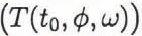 , is measured over a large temperature range. But the magnitude of temperature change at GISP2 during the Holocene is small compared to this range, so a local test of Equation (2) in the vicinity of the GISP2 site is warranted. However, our attempt to define a local spatial gradient is inconclusive (Fig. 6). This may indicate that no clear local spatial gradient exists. It certainly indicates that a lot of effort can be spent drilling shallow cores, measuring their isotopic composition and measuring temperatures without learning anything about the δ
18O-temperature relationship. In addition, the comparison of 10 m or 20 m temperature with decades-averaged isotopes is not perfect, because the temperature at a given depth is a variably weighted average of surface temperatures over some time period. We are unsure how, in a changing climate, to average isotopes to make this comparison valid.
Given this uncertainty in what averaging time should be used, and the scatter of our data, it seems clear that the borehole calibration is an easier method for finding the δ-T relationship than is measuring spatial gradients in the vicinity of coring sites. The borehole calibration only requires measuring temperatures in the one hole drilled for the paleoclimate study, and leads to a clearly defined relationship between δ and temperature in this case. Borehole calibrations should be successful as long as the temperature profile has significant non-steady character, with deviations much larger than measurement error.
Furthermore, although the analytic uncertainty in mean annual δ 18O values is small, intercomparison of adjacent ice cores demonstrates a variability in mean annual values of as much as 1.0%o, suggesting that δ 18O may be reliable as a thermometer only when averaged over decades or longer (e.g. Reference Benoist, Jouzel, Lorius, Merlivat and PourchetBenoist and others, 1982; personal communication from D. Dahl-Jensen). Heat-transport processes provide this smoothing naturally, so borehole temperatures are well suited for calibrations of Equation (1). Moreover, the true relation between mean annual δ 18O and Τ may change with time, due to changes in the seasonality of accumulation (Reference Fisher, Koerner, Paterson, Dansgaard, Gundestrup and ReehFisher and others, 1983) or changes in vapor-source area and transport paths (Reference Dansgaard, White and JohnsenDansgaard and others, 1989). Borehole calibrations will give values for a and b that best average these effects over time, whereas modern spatial gradients will not include these effects at all. Unlike spatial gradient calibrations, borehole calibrations do not rely on the truth of Equation (2), which has been shown to be incorrect in at least one case (Reference Peel, Mulvaney and DavisonPeel and others, 1988).
Conclusion
For conversion of GISP2 δ 18O records to temperature histories, we recommend using Equation (1) with the coefficient a in the interval (0.45,0.66), and with the corresponding b value given by Equation (2). This calibration is applicable to at least the most recent five or six centuries of isotope data.
We have shown that we can achieve a clearly defined calibration of an isotopic paleothermometer using borehole temperatures, in one case. Unlike calibrations based on other methods, borehole-temperature calibrations apply for an extended period of time at one location. For this reason and, because these calibrations require little additional cost or effort,borehole-temperature calibrations should be a regular part of ice-core paleoclimate studies that utilize isotopic paleothermometers.
Acknowledgements
We thank B. Koci, G. Jablunovsky, J. Fitzpatrick, K. Taylor, C. Alley, T. Saling, E. Steig, J. White, L. Barlow, C. Massey, other GISP2 participants, the Polar Ice Coring Office and and the GISP2 Science Management Office. We thank D. Dahl-Jensen for her stimulating insights. D. MacAyeal, A. Taylor, K. Wang and an anonymous reviewer also provided helpful comments on this work. This research was supported in part by the U.S. National Science Foundation under grants DPP-8822027 to R.B.A., DPP-8822073 to P.M.G. and DPP-8520855 and DPP-8822081 to J.B., and by a fellowship from the David and Lucile Packard Foundation to R.B.A. K.M.C. gratefully acknowledges the financial support of the Westinghouse Corporation, Chevron USA and The Pennsylvania State University. This paper is based, in part, upon work supported under a U.S. National Science Foundation Graduate Research Fellowship.
The accuracy of references in the text and in this list is the responsibility of the authors, to whom queries should be addressed.



