



1. Introduction
Reducing the skin-friction drag in wall turbulence is of great importance in improving the speed and fuel efficiency of aeroplanes, underwater vehicles and many other means of transportation. To reduce drag, numerous control strategies have been studied (Corke & Thomas Reference Corke and Thomas2018; Chung et al. Reference Chung, Hutchins, Schultz and Flack2021; Ricco et al. Reference Ricco, Skote and Leschziner2021; Fukagata et al. Reference Fukagata, Iwamoto and Hasegawa2024). Control methods that do not require any input energy are usually implemented by changing the surface condition, which adjusts the turbulence structure near the wall, such as through riblets (Choi et al. Reference Choi, Moin and Kim1993; Bechert et al. Reference Bechert, Bruse, Hage, Van der Hoeven and Hoppe1997; Gatti et al. Reference Gatti, von Deyn, Forooghi and Frohnapfel2020; Modesti et al. Reference Modesti, Endrikat, Hutchins and Chung2021), superhydrophobic surfaces (Rothstein Reference Rothstein2010; Checco et al. Reference Checco, Ocko, Rahman, Black, Tasinkevych, Giacomello and Dietrich2014; Park et al. Reference Park, Sun and Kim2014; Rastegari & Akhavan Reference Rastegari and Akhavan2018) and roughness elements (Jimenez Reference Jimenez2004; Chung et al. Reference Chung, Hutchins, Schultz and Flack2021). In the case of riblets, tiny sizes are required for drag reduction, which means that they are easily eroded by atmospheric dust (Ricco et al. Reference Ricco, Skote and Leschziner2021). For superhydrophobic surfaces, drag reductions of up to 50 % for the turbulent channel (Rothstein Reference Rothstein2010) and 75 % for the turbulent boundary layer (Park et al. Reference Park, Sun and Kim2014) are obtained in laboratories, but a high shear rate or pressure can easily destroy superhydrophobic surfaces (Checco et al. Reference Checco, Ocko, Rahman, Black, Tasinkevych, Giacomello and Dietrich2014; Rastegari & Akhavan Reference Rastegari and Akhavan2018). These issues limit the practical application of passive surface control.
When an external excitation is introduced, the self-sustaining cycle of near-wall vortices is expected to break and hence lead to drag reduction (Kim & Bewley Reference Kim and Bewley2007; Chung & Talha Reference Chung and Talha2011; Deng & Xu Reference Deng and Xu2012; Mamori et al. Reference Mamori, Iwamoto and Murata2014). Typical operations include wall oscillations and streamwise travelling waves (Jung et al. Reference Jung, Mangiavacchi and Akhavan1992; Quadrio et al. Reference Quadrio, Ricco and Viotti2009; Agostini et al. Reference Agostini, Touber and Leschziner2014; Yakeno et al. Reference Yakeno, Hasegawa and Kasagi2014; Chandran et al. Reference Chandran, Zampiron, Rouhi, Fu, Wine, Holloway, Smits and Marusic2023; Deshpande et al. Reference Deshpande, Chandran, Smits and Marusic2023; Rouhi et al. Reference Rouhi, Fu, Chandran, Zampiron, Smits and Marusic2023) and blowing/suction control (Choi et al. Reference Choi, Moin and Kim1994; Sumitani & Kasagi Reference Sumitani and Kasagi1995; Kametani & Fukagata Reference Kametani and Fukagata2011; Guseva & Jiménez Reference Guseva and Jiménez2022). For travelling-wave methods, a wide range of parameter searches have been performed to explore the optimal drag reduction when the Reynolds number (
 $\textit{Re}$
) changes, and a prediction for a high-drag-reduction
 $\textit{Re}$
has been given based on scaling models (Hurst et al. Reference Hurst, Yang and Chung2014; Gatti & Quadrio Reference Gatti and Quadrio2016). For blowing and suction control, imposing a specific wall velocity to counteract the sweep and ejection effects produced by streamwise vortices in the buffer layer can reduce drag by 25 % at moderate friction Reynolds numbers of
 $\textit{Re}_\tau =110$
–
 $180$
(Choi et al. Reference Choi, Moin and Kim1994; Deng et al. Reference Deng, Xu, Huang and Cui2014). As it is difficult to determine the appropriate wall velocity in the buffer layer in real-time control, Park & Choi (Reference Park and Choi2020) developed convolutional neural networks to construct a map between the appropriate wall velocity and various wall parameters. Subsequent work in this direction by Han & Huang (Reference Han and Huang2020) resulted in drag reduction of
 $15\,\%$
for
 $\textit{Re}_\tau =390$
–
 $580$
.
In numerical studies, flow control is excited by applying a body force (Ricco et al. Reference Ricco, Skote and Leschziner2021) in the Navier–Stokes equations. Schoppa & Hussain (Reference Schoppa and Hussain1998) added body forces to the Fourier space to induce counter-rotating streamwise swirls in channels at
 $\textit{Re}_\tau =100$
. Later, counter-rotating swirls at higher
 $\textit{Re}$
were employed by Canton et al. (Reference Canton, Örlü, Chin and Schlatter2016) and Yao et al. (Reference Yao, Chen and Hussain2018), and a
 $15\,\%$
drag reduction was obtained at
 $\textit{Re}_\tau =550$
by adjusting the wall-normal location of the controlling swirls. A series of numerical studies by Schoppa & Hussain (Reference Schoppa and Hussain1998), Canton et al. (Reference Canton, Örlü, Chin and Schlatter2016) and Yao et al. (Reference Yao, Chen and Hussain2018) inspired experimental investigations using synthetic wall jets (Iuso et al. Reference Iuso, Onorato, Spazzini and Di Cicca2002; Cannata et al. Reference Cannata, Cafiero and Iuso2020) and plasma actuation (Thomas et al. Reference Thomas, Corke, Hussain, Duong, McGowan, Jasinski and Simmons2016; Cheng et al. Reference Chen, Yao and Hussain2021; Duong et al. Reference Duong, Corke and Thomas2021). Recently, large-scale control strategies on rough walls have been investigated by Duan et al. (Reference Duan, Chen, Ji, Yao and Hussain2024) and Nozarian et al. (Reference Nozarian, Abkar and Forooghi2024), and robust drag reduction has been achieved at the moderate value of
 $\textit{Re}_\tau =180$
.
As
 $\textit{Re}$
increases, large-scale outer movements contribute more to skin friction (de Giovanetti et al. Reference de Giovanetti, Hwang and Choi2016). An experimental study on the control of these structures (Marusic et al. Reference Marusic, Chandran, Rouhi, Fu, Wine, Holloway, Chung and Smits2021) reported a significant 13 % drag reduction and 10 % net power saving at
 $\textit{Re}_\tau =12\,800$
. In these experiments, the spanwise wall oscillation frequency was lowered to produce the effective suppression of flow structures with relatively large wavelengths, resulting in notable drag reduction for a small energy input. The idea of large-scale wall opposition control has been applied at
 $\textit{Re}_\tau =932$
to enhance the intensity or mixing of turbulence (Guseva & Jiménez Reference Guseva and Jiménez2022). Recently, direct numerical simulations (DNS) of spanwise wall oscillations have been extended to high Reynolds numbers. Xiao et al. (Reference Xiao, Ceci, Orlandi and Pirozzoli2024) conducted a DNS study of rotating pipes with
 $\textit{Re}_\tau$
up to 3000, and observed the suppression of large-scale motions associated with a very high drag reduction. For rough walls, Deshpande et al. (Reference Deshpande, Kidanemariam and Marusic2024) showed that spanwise wall oscillations can yield drag reduction of up to 25 %. However, in open channels, the DNS conducted by Gatti et al. (Reference Gatti, Quadrio, Chiarini, Gattere and Pirozzoli2025) for
 $\textit{Re}_\tau \approx 6000$
suggested that the drag reduction rate decreases with increasing
 $\textit{Re}$
, regardless of the control parameters of the spanwise wall oscillations.
In addition to numerical and laboratory experiments, several theoretical frameworks have been developed in which the drag coefficient is represented through volume integration of different mean quantities. Using the mean momentum equation, the Fukagata–Iwamoto–Kasagi (FIK) identity (Fukagata et al. Reference Fukagata, Iwamoto and Kasagi2002) was obtained and used to analyse the drag contributions of (equivalent) laminar and turbulent motions (Yudhistira & Skote Reference Yudhistira and Skote2011; de Giovanetti et al. Reference de Giovanetti, Hwang and Choi2016; Yoon et al. Reference Yoon, Ahn and Hwang2016). Floryan (Reference Floryan2023) further argued that the laminarisation of the flow results in a limit for the potential drag reduction in turbulent channels. In view of energy dynamics, Renard & Deck (Reference Renard and Deck2016) decomposed
 $C_{\!f}$
into the integral of the mean flow dissipation and turbulent production; this formulation has been extended to compressible flows (Li et al. Reference Li, Fan, Modesti and Cheng2019) and rough walls (Zhang et al. Reference Zhang, Yang, Chen and Wan2024). Analysis of the energy flux introduced by Gatti et al. (Reference Gatti, Cimarelli, Hasegawa, Frohnapfel and Quadrio2018) led to a dissipation-based expression for
 $C_{\!f}$
(Chen et al. Reference Chen, Yao and Hussain2021). Roccon et al. (Reference Roccon, Zonta and Soldati2021) used a similar framework to analyse drag reduction in turbulent lubricated channel flows. Recently, Zhao et al. (Reference Zhao, Fan and Li2024) proposed a drag decomposition based on velocity–vorticity correlations, and investigated the physical relations between the generation of wall friction and vortical motions.
Despite the studies mentioned above, there is still a gap between academic research and practical applications. A major difficulty lies in the decreasing efficacy of drag reduction at high
 $\textit{Re}$
(Corke & Thomas Reference Corke and Thomas2018; Ricco et al. Reference Ricco, Skote and Leschziner2021). While different strategies have their own character, combining the merits of different strategies together appears to be a new direction. The current work aims to verify the efficacy of composite drag control (CDC) by combining the active excitations of opposition flows and large-scale swirls. The underlying mechanism is that large-scale swirls merge near-wall streaks and suppress the generation of streamwise vortices (Waleffe Reference Waleffe1997; Jiménez & Pinelli Reference Jiménez and Pinelli1999), and the secondary flows between the colliding motions could be further inhibited by blowing and suction, resulting in a greater reduction in drag. This idea was tested in our preliminary study but only at a single Reynolds number of
 $\textit{Re}_\tau \approx 200$
(Yao et al. Reference Yao, Chen and Hussain2021). In this study, we performed a wider search for parameters and considered the
 $\textit{Re}_\tau$
trend of drag reduction at
 $\textit{Re}_\tau =180$
,
 $395$
and
 $550$
. Interestingly, we find a significant and robust drag reduction of more than 28 % for all Reynolds numbers, demonstrating the potential of additive and synergistic control methods. The results thus offer a composite perspective for the development of effective drag controls.
The paper is organised as follows. The numerical scheme and control methods are presented in § 2. Mean flow statistics and coherent structures are examined in § 3 to elucidate the underlying physics of drag control. Section 4 introduces the spectrum analysis and proper orthogonal decomposition (POD), while § 5 is devoted to the vortical decomposition of skin friction. The concluding remarks are given in § 6.
2. Computational set-up
2.1. Control schemes
Schematic for CDC, which combines SOJF and OC. Note that SOJF generates large-scale swirls which transport velocity streaks (blue contours) into the middle span and merges them together; OC further weakens the streak envelopes via surface blowing and suction.

The governing equations for incompressible turbulent channel flow are the Navier–Stokes equations:
 \begin{align} \partial _i u_i & = 0,\end{align}
 \begin{align} \partial _t {{u_i}}+\partial _{\!j} {{u_iu_{\!j}}} & = \nu \partial _{\!j}\partial _{\!j} { {u_i}}- \partial _i{p}/\rho +F_i, \end{align}
where the subscript
 $i$
denotes the direction (
 $x$
,
 $y$
,
 $z$
) in Cartesian coordinates;
 $u_i$
is the corresponding velocity in the streamwise, wall-normal and spanwise directions;
 $\nu$
is the fluid kinematic viscosity;
 $p$
is the pressure;
 $\rho$
is the density; and
 $F_i$
is the external volume force. Following previous studies (Yao et al. Reference Yao, Chen and Hussain2018; Ricco et al. Reference Ricco, Skote and Leschziner2021), the volume force, referred to as the spanwise opposed wall-jet force, is set as
 \begin{eqnarray} F_x=F_y=0; \quad F_z=A_s\sin (\beta z)g(y), \end{eqnarray}
where
 $A_s$
is the forcing amplitude;
 $\beta$
(
 $=2\pi /\lambda$
) is the spanwise wavenumber; and
 $g(y)$
is a dimensionless function. In this paper, the friction velocity and viscous length of uncontrolled flow (indicated by subscript 0) are used to non-dimensionalise all control parameters: (a)
 $A^+_s=A_s\nu /u^3_{\tau ,0}$
; (b)
 $\lambda ^+=2\pi /\beta ^+$
(
 $\beta ^+=\beta \nu /u_{\tau ,0}$
); (c)
 $g(y^+)=y^+\exp (-\eta y^{+2})$
,
 $y^+=yu_{\tau ,0}/\nu$
; where
 $\eta$
is the decay factor determining the wall-normal velocity profile of the wall jet. The function
 $g$
reaches its maximum at
 $y^{+}=y^+_c=1/\sqrt {2\eta }$
, and its maximum value
 $y^+_c\exp (-1/2)$
is used to normalise
 $g(y)$
.
The current work investigates a more efficient control method by combining large-scale spanwise opposed wall-jet forcing (SOJF) with opposition control (OC) (Choi et al. Reference Choi, Moin and Kim1994; Kametani & Fukagata Reference Kametani and Fukagata2011; Guseva & Jiménez Reference Guseva and Jiménez2022), with the expectation that OC will further eliminate small-scale vortices that escape from the control of SOJF. Therefore, in addition to the forcing in (2.3), the wall-normal velocity at the wall is set as
 \begin{eqnarray} v_w(x,z,t)=- v(x,y_d,z,t), \end{eqnarray}
where
 $ v(y_d)$
is the wall-normal velocity at the detection plane
 $y^+_d=15$
(hereinafter, the subscript
 $w$
represents the value on the wall). For compatibility with the forcing in (2.3), such a wall-velocity setting is imposed only on the bottom wall. A sketch of CDC for a channel is shown in figure 1.
2.2. Simulation parameters
The current DNS is conducted using the code of ‘Simson’ developed by Lundbladh et al. (Reference Lundbladh, Henningson and Johansson1992), Chevalier et al. (Reference Chevalier, Schlatter, Lundbladh and Henningson2007) and Schlatter et al. (Reference Schlatter, Li, Brethouwer, Johansson and Henningson2010). The code is based on the spectral integration technique. In the streamwise and spanwise directions, periodic boundary conditions are employed, and in the wall-normal direction, the boundary condition is equation (2.4). Fourier series are adopted for spatial discretisation in the wall-parallel directions, and in the wall-normal direction, Chebyshev series are used. A third-order Runge–Kutta scheme is applied for time integration of the advective and forcing terms. The Crank–Nicolson method for viscous terms is adopted in the streamwise and spanwise directions. By adjusting the mean pressure gradient, the bulk velocity
 $U_b$
is kept constant. Three bulk Reynolds numbers, i.e.
 $\textit{Re}_b=2800$
,
 $6800$
and
 $10\,000$
, are set to obtain simulations with
 $\textit{Re}_\tau =180$
,
 $395$
and
 $550$
, respectively. Table 1 lists the domain sizes, spatial resolution and simulation times. The initial condition in all simulations is an uncontrolled, fully developed turbulent velocity field at the same
 $\textit{Re}_\tau$
.
Details of the numerical discretisation employed in the present simulations, including uncontrolled channel (CH), control with wall oscillations (OC), large-scale swirls (SOJF) and composite excitations (CDC). The numerical discretisation is the same for all CDC cases, and the drag reduction rate
 $R$
and net power saving
 $N$
are only given for the optimal control parameters marked in figure 2.

Table 1. Long description
A table comparing numerical discretization parameters for different simulation cases. The table has 12 rows and 10 columns. Column headers are: Case, Re_b, L_x/h, L_z/h, N_x x N_y x N_z, Δy+_w, Δy+_max, Tu/T, R %, (ΔR %) and N %. Row 1: Case, CH180; Re_b, 2800; L_x/h, 4π; L_z/h, 2π; N_x x N_y x N_z, 192 x 129 x 128; Δy+_w, 0.05; Δy+_max, 4.4; Tu/T, 42.8; R %, 0; (ΔR %), (—); N %, —. Row 2: Case, OC180; Re_b, 2800; L_x/h, 4π; L_z/h, 2π; N_x x N_y x N_z, 192 x 129 x 128; Δy+_w, 0.05; Δy+_max, 3.9; Tu/T, 37.8; R %, 22; (ΔR %), (0.7); N %, 21.5. Row 3: Case, SOJF180; Re_b, 2800; L_x/h, 4π; L_z/h, 2π; N_x x N_y x N_z, 192 x 129 x 128; Δy+_w, 0.05; Δy+_max, 4.0; Tu/T, 38.8; R %, 18; (ΔR %), (1.1); N %, 15. Row 4: Case, CDC180; Re_b, 2800; L_x/h, 4π; L_z/h, 2π; N_x x N_y x N_z, 192 x 129 x 128; Δy+_w, 0.04; Δy+_max, 3.6; Tu/T, 34.8; R %, 34; (ΔR %), (2.0); N %, 33. Row 5: Case, CH395; Re_b, 6800; L_x/h, 2π; L_z/h, π; N_x x N_y x N_z, 256 x 161 x 192; Δy+_w, 0.07; Δy+_max, 7.6; Tu/T, 52.9; R %, 0; (ΔR %), (—); N %, —. Row 6: Case, OC395; Re_b, 6800; L_x/h, 2π; L_z/h, π; N_x x N_y x N_z, 256 x 161 x 192; Δy+_w, 0.07; Δy+_max, 6.8; Tu/T, 34.0; R %, 19; (ΔR %), (0.5); N %, 18.6. Row 7: Case, SOJF395; Re_b, 6800; L_x/h, 2π; L_z/h, π; N_x x N_y x N_z, 256 x 161 x 192; Δy+_w, 0.07; Δy+_max, 6.9; Tu/T, 34.3; R %, 18; (ΔR %), (0.6); N %, 15. Row 8: Case, CDC395; Re_b, 6800; L_x/h, 2π; L_z/h, π; N_x x N_y x N_z, 256 x 161 x 192; Δy+_w, 0.06; Δy+_max, 6.3; Tu/T, 31.4; R %, 31; (ΔR %), (2.3); N %, 29. Row 9: Case, CH550; Re_b, 10000; L_x/h, π; L_z/h, 2π/3; N_x x N_y x N_z, 256 x 193 x 192; Δy+_w, 0.07; Δy+_max, 8.9; Tu/T, 36.5; R %, 0; (ΔR %), (—); N %, —. Row 10: Case, OC550; Re_b, 10000; L_x/h, π; L_z/h, 2π/3; N_x x N_y x N_z, 256 x 193 x 192; Δy+_w, 0.07; Δy+_max, 8.2; Tu/T, 32.6; R %, 20; (ΔR %), (1.4); N %, 19.8. Row 11: Case, SOJF550; Re_b, 10000; L_x/h, π; L_z/h, 2π/3; N_x x N_y x N_z, 256 x 193 x 192; Δy+_w, 0.07; Δy+_max, 8.2; Tu/T, 33.6; R %, 16; (ΔR %), (1.4); N %, 13. Row 12: Case, CDC550; Re_b, 10000; L_x/h, π; L_z/h, 2π/3; N_x x N_y x N_z, 256 x 193 x 192; Δy+_w, 0.06; Δy+_max, 7.6; Tu/T, 62.2; R %, 28; (ΔR %), (1.3); N %, 26.
Drag reduction
 $R$
is defined as
 \begin{equation} R=(1-C^{\textit{control}}_{\!f}/C_{f,0})\times 100\,\%, \end{equation}
where
 $C_{\!f}$
is evaluated by the friction force (
 $\tau _w$
) at the bottom wall, i.e.
 \begin{equation} C_{\!f}/2=\tau _w/(\rho U^2_b)=U^{+2}_b. \end{equation}
The uncertainty of
 $R$
is calculated following the procedure described by Gatti & Quadrio (Reference Gatti and Quadrio2016), i.e.
 $\sigma _R =(C_{\!f}/C_{f,0}\sqrt {(\sigma _{C_{f,0}}/C_{f,0})^2+(\sigma _{C_{\!f}}/C_{\!f})^2})$
. Here,
 $\sigma _{C_{f}}$
is the standard uncertainty of
 $C_{\!f}$
using an autoregressive method (Oliver et al. Reference Oliver, Malaya, Ulerich and Moser2014) and
 $\sigma _R$
is the uncertainty of
 $R$
by propagating the standard uncertainty of
 $C_{\!f}$
. The uncertainty is finally extended to a 95 % confidence interval by
 $\delta R=1.96 \sigma _R$
. The calculated uncertainty of
 $R$
is listed in table 1.
The net power-saving rate
 $N$
is defined as
 \begin{equation} N\equiv (1-(P+P^{\textit{in}})/P_0)\times 100\,\%, \end{equation}
where
 $P=u_\tau ^2U_b/h$
and
 $P_0=u_{\tau ,0}^2U_b/h$
are the total pumping powers of the controlled and uncontrolled channels, respectively, and
 $P^{\textit{in}}$
is the input power of the control excitation. In (2.7), the power input is
 \begin{equation} P^{\textit{in}} = \big \langle {wF_z}\big \rangle + \big \langle {\rho v_{w}^3/2}\big \rangle + \big \langle {p_{w}v_{w}}\big \rangle , \end{equation}
where
 $\langle {wF_z}\rangle$
is the power input corresponding to SOJF (Chen et al. Reference Chen, Yao and Hussain2021) and
 $\langle {\rho v_{w}^3/2}\rangle + \langle {p_{w}v_{w}}\rangle$
is the energy injected into channel from the wall by OC (Gatti et al. Reference Gatti, Cimarelli, Hasegawa, Frohnapfel and Quadrio2018). The net power-saving rate
 $N$
obtained from (2.7) is listed in the last column of table 1.
2.3. Parameter search
Drag reduction (
 $R$
) of CDC in the
 $A_s^+{-}y_c^+$
plane for (a)
 $\textit{Re}_\tau =180$
, (b)
 $\textit{Re}_\tau =395$
and (c)
 $\textit{Re}_\tau =550$
. The symbol
 $\bullet$
(black) denotes the specific control parameters under CDC. A total of 114 simulations were performed. In each panel, the symbol
 $+$
(red) denotes the optimal control parameters which yield the largest
 $R$
for the corresponding
 $\textit{Re}_\tau$
.

After adding OC, the optimal forcing amplitude is no longer the same as the value set for SOJF. Thus, a parameter search is performed for each different forcing amplitude and control height. Figures 2(a)–2(c) show the drag reduction
 $R$
as a function of
 $A^+_s$
and
 $y^+_c$
at
 $\textit{Re}_\tau = 180$
,
 $395$
and
 $550$
, respectively. Simulations are carried out at
 $A^+_s=[1, 2, 3, 4, 5, 6]\times 0.00303$
and
 $y^+_c=[25, 30, 35, 40, 45, 50, 55]$
for
 $\textit{Re}_\tau =180$
;
 $A^+_s=[3, 4, 5, 6, 7, 8]\times 0.00181$
and
 $y_c^+=[35, 40, 45, 50, 55, 60]$
for
 $\textit{Re}_\tau =395$
;
 $A^+_s=[7, 8, 9, 10, 11, 12]\times 0.00136$
and
 $y_c^+=[45, 50, 55, 60, 65, 70]$
for
 $\textit{Re}_\tau =550$
. Hence,
 $114$
simulations are performed for CDC, covering a wide range of
 $A_s^+$
and
 $y_c^+$
.
In figure 2, the contours are computed from a linear interpolation of the discrete simulated points. It is impressive that a high value of
 $R$
can be obtained in broad ranges of the forcing amplitude and the control height. The optimal values of
 $A_s^+$
are almost independent of the Reynolds number, i.e. 0.009, 0.011, 0.011 for increasing
 $\textit{Re}_\tau$
. This suggests a typical velocity of about
 $4u_\tau$
for the spanwise wall jets, consistent with the plasma experiments conducted by Thomas et al. (Reference Thomas, Corke, Hussain, Duong, McGowan, Jasinski and Simmons2016) and Corke & Thomas (Reference Corke and Thomas2018). Moreover, according to the FIK identity (Fukagata et al. Reference Fukagata, Iwamoto and Kasagi2002), Reynolds shear stress contributes to the turbulent part of
 $C_{\!f}$
, the suppression of which decreases drag. This is consistent with our optimal
 $y^+_c$
, i.e. 40 for
 $\textit{Re}_\tau =180$
, 50 for
 $\textit{Re}_\tau =395$
and 65 for
 $\textit{Re}_\tau =550$
, which follows the
 $\textit{Re}_\tau$
scaling of the Reynolds shear stress peak location (Chen et al. Reference Chen, Hussain and She2019). For
 $\beta$
,
 $\lambda ^+=2\pi /\beta \approx 1200$
under all controls, implying a simultaneous control of
 $10$
–
 $12$
velocity streaks (because their spanwise spacing is
 $\lambda ^+_z\approx 100$
(see e.g. Del Alamo & Jimenez Reference Del Alamo and Jimenez2006)) by a pair of counter-rotating streamwise swirls. Compared with the pure SOJF control, the optimal
 $A^+_s$
is slightly smaller under CDC and the optimal
 $y_c^+$
is larger. This is because OC weakens the near-wall streaks and shifts the Reynolds shear stress peak outward, as explained later herein.
The maximum drag reduction (
 $R$
) and the net power saving (
 $N$
) obtained by CDC at
 $\textit{Re}_\tau =180$
are 34 % and 33 %, respectively (table 1), slightly higher than in our preliminary study (Yao et al. Reference Yao, Chen and Hussain2021). In the
 $\textit{Re}_\tau$
range considered here, although
 $R$
decreases with increasing
 $\textit{Re}_\tau$
, CDC still produces a 28 % drag reduction at
 $\textit{Re}_\tau =550$
, much higher than
 $20\,\%$
of OC and 16 % of SOJF. In the following, the optimal control cases are analysed in detail to understand the drag reduction performance.
3. Results of mean flow statistics
3.1. Mean velocity and Reynolds stresses
Mean velocity profile along wall-normal direction at
 $\textit{Re}_\tau =550$
for (a) the bottom half-channel and (b) the top half-channel. The superscripts
 $+$
and
 $\#$
indicate normalisation by the bottom and top wall-friction velocities, respectively.

Reynolds stresses under various controls compared with uncontrolled case (black solid line) at
 $\textit{Re}_\tau =550$
: (a)
 $\langle u'u'\rangle ^+$
, (b)
 $\langle v'v'\rangle ^{+}$
, (c)
 $\langle |u'v'|\rangle ^{+}$
and (d)
 $\langle w'w'\rangle ^+$
. Here OC is represented by the yellow solid line. For SOJF (blue) and CDC (red), the solid line corresponds to random fluctuations and the dashed line corresponds to coherent fluctuations.

According to (2.6), the volume-integrated mean velocity determines the drag coefficient. Taking
 $\textit{Re}_\tau =550$
as an example, the mean velocity profiles across the bottom half-channel are shown in figure 3(a). For OC (yellow line), the logarithmic mean profile is preserved with the same slope as that of uncontrolled flow (black line), but its intercept increases due to a thicker buffer layer (Kametani & Fukagata Reference Kametani and Fukagata2011; Chung et al. Reference Chung, Hutchins, Schultz and Flack2021). In contrast, SOJF (blue line) flattens the mean velocity in the bulk due to the large-scale swirls that homogenise the shear. It is clear that the CDC (red line) resembles the SOJF feature by further lifting the mean profile and therefore yields the smallest
 $C_{\!f}$
. As the velocity changes little for the upper half-channel (figure 3
b), hereafter we focus on the flow alteration in the lower one.
A common understanding of drag reduction is that turbulent fluctuations must be suppressed, which is reflected in the smaller Reynolds stresses under control (Jeong et al. Reference Jeong, Hussain, Schoppa and Kim1997; Jiménez & Pinelli Reference Jiménez and Pinelli1999; Guseva & Jiménez Reference Guseva and Jiménez2022). Nevertheless, the current study calls for caution on this point of view, because of the proper Reynolds decomposition needed. For SOJF and CDC, if following the usual Reynolds decomposition by averaging over
 $txz$
ensembles, the motions of counter-rotating swirls would be mistreated as turbulent fluctuations and lead to larger Reynolds stresses even under significant drag reduction. Therefore, to distinguish random flow motions from coherent large-scale swirls, it is more reasonable to perform a triple decomposition (Chen et al. Reference Chen, Yao and Hussain2021), i.e.
 \begin{eqnarray} u_i=\overline {u}_i+\tilde {u}_i+u'',\quad u''_i=u'_i-\tilde {u}_i, \end{eqnarray}
where
 \begin{eqnarray} \tilde {u}_i=\langle u_i \rangle _{xt}-\overline {u}_i. \end{eqnarray}
Here, the subscript
 $xt$
indicates averaging the streamwise and time ensembles;
 $\overline {u}$
is the usual Reynolds-averaged mean velocity;
 $\tilde {u}$
represents the coherent motions induced by the SOJF in the
 $y$
–
 $z$
plane, which are closely associated with the controlling swirls; and
 $u''$
is the random turbulent fluctuation. To explain, for flow without control or with OC,
 $u''$
is the same as the Reynolds decomposition
 $u'$
because
 $\tilde {u}$
is zero and therefore there is no need for trip decomposition.
Using the triple decomposition above, SOJF and CDC induce coherent stresses
 $\langle \tilde {u}_i\tilde {u}_{\!j}\rangle ^+$
and random stresses
 $\langle u''_iu''_{\!j}\rangle ^+$
, which are represented by dashed and solid lines, respectively, shown in figure 4. In particular, figure 4(a) shows that
 $\langle u''u''\rangle ^+$
of SOJF or CDC is uniformly lower than
 $\langle u'u'\rangle ^+$
of no control (solid black line). Yet, the sum of
 $\langle u''u''\rangle ^+$
and
 $\langle \tilde {u}\tilde {u}\rangle ^+$
, which is the usual Reynolds-averaged stress
 $\langle u'u'\rangle ^+$
, is obviously higher than
 $\langle u'u'\rangle ^+$
without control. Similar observations can be made for the other stress components (figure 4
b–d). Therefore, it is important to exclude coherent motions when highlighting the lower turbulence intensity under drag reduction.
Two notable points for CDC deserve further discussion from figure 4. First, compared with SOJF, coherent motions are weaker under CDC. This is drawn from figure 4(a,c,d), where CDC-C (dashed red line) is lower than SOJF-C (dashed blue line) throughout the flow domain. This conforms to the optimal
 $A^+_s$
shown in figure 2, which is smaller for CDC than for SOJF, because
 $A^+_s$
represents the strength of coherent swirls. Second, compared with OC, random fluctuations are suppressed under CDC. This is concluded from figure 4 where CDC-R (solid red line) is uniformly lower than OC (solid yellow line). We also observe the effect of the virtual wall under CDC similar to that of OC (Chung & Talha Reference Chung and Talha2011; Deng et al. Reference Deng, Xu, Huang and Cui2014), namely at
 $y^+\approx 5$
,
 $\langle v'v'\rangle ^{+}=0$
(figure 4
b) and
 $\langle |u'v'|\rangle ^{+}=0$
(figure 4
c). From these comparisons, it is well illustrated that CDC combines the advantages of SOJF and OC together, thus generating the largest drag reduction.
Pre-multiplied spectra of streamwise fluctuation intensity
 $k_z\varPhi _{uu}(y^+,k_z^+)/u_\tau ^2$
(a,c,e) and co-spectrum of Reynolds shear stress
 $k_z\varPhi _{uv}(y^+,k_z^+)/u_\tau ^2$
(b,d, f): (a,b) flow without control, (c,d) flow with CDC, and the coherent
 $k_z\varPhi _{\tilde {u}\tilde {u}}(y^+,k_z^+)/u_\tau ^2$
(e) and
 $k_z\varPhi _{\tilde {u}\tilde {v}}(y^+,k_z^+)/u_\tau ^2$
( f) for flow with CDC.

To show that near-wall random turbulent structures are suppressed by the large-scale swirls, the pre-multiplied spectra of
 $k_z\varPhi _{uu}(y^+, k_z^+)/u_\tau ^2$
and
 $k_z\varPhi _{uv}(y^+, k_z^+)/u_\tau ^2$
are shown in figure 5. Without control (figure 5
a), the maximum of
 $k_z\varPhi _{uu}/u_\tau ^2$
is located at
 $y^+\approx 15$
and
 $\lambda _z^+\approx 100$
, where
 $\lambda _z^+=2\pi /k_z^+$
is wavelength. The value
 $y^+\approx 15$
corresponds to the inner peak of random
 $\langle u'u'\rangle ^+$
shown in figure 4(a), while
 $\lambda _z^+\approx 100$
corresponds to the width of the velocity streaks (Schoppa & Hussain Reference Schoppa and Hussain2002; Jimenez & Hoyas Reference Jimenez and Hoyas2008). Under CDC (figure 5
c), the wall-normal location of the spectrum peak shifts outward and the corresponding wavelength becomes
 $\lambda _z^+\approx 1000$
. Similarly, without control (figure 5
b),
 $k_z\varPhi _{uv}/u_\tau ^2$
has a peak at
 $y^+\approx 30$
(Chen et al. Reference Chen, Hussain and She2019); under CDC, the peak moves outward to
 $y^+\approx 65$
(figure 5
d). The value of
 $y^+\approx 65$
corresponds to the optimal control height
 $y_c^+$
in figure 2(c), and the wavelength
 $\lambda _z^+\approx 1000$
is the spacing between large-scale swirls. A small contour island appears at
 $y^+\approx 30$
and
 $\lambda _z^+\approx 100$
in figure 5(d), implying the contribution of the remnant small-scale streaks to the Reynolds shear stress near the wall. The pre-multiplied spectra of coherent motions, i.e.
 $k_z\varPhi _{\tilde {u}\tilde {u}}/u_\tau ^2$
and
 $k_z\varPhi _{\tilde {u}\tilde {v}}/u_\tau ^2$
, are shown in figures 5(e) and 5( f), respectively. The near-peak distributions of figures 5(e) and 5( f) are very similar to those shown in figures 5(c) and 5(d), except that the small-scale contour islands are absent. This indicates that
 $\tilde {u}$
and
 $\tilde {v}$
obtained from the triple decomposition can effectively represent the large-scale coherent swirls.
3.2. Mean wall shear stress
Spanwise variation of mean wall shear stress
 $\tau _w$
for SOJF (blue), OC (yellow), and CDC (red) normalised by uncontrolled wall stress at (a)
 $\textit{Re}_\tau =180$
, (b)
 $395$
and (c)
 $550$
.

Another inspiring way to understand the drag variation is to examine the mean shear stress (after
 $tx$
-averaging) on the wall, shown in figure 6 for the current three
 $\textit{Re}_\tau$
values. For OC,
 $\tau _w/\tau _{w,0}$
is homogeneous along the spanwise direction and plateaus at
 $0.8$
; for SOJF, there is a hump in the middle span (
 $z/L_z=0.5$
) where the magnitude increases moderately with increasing
 $\textit{Re}_\tau$
; for CDC, the wall shear stress is flattened and has a lower magnitude than under OC, which is around
 $\tau _w/\tau _{w,0}\approx 0.7$
.
The
 $\lambda _2$
vortical structures plotted against the background of streamwise velocity contours in the plane of
 $y^+= 15$
for flow with (a) no control, (b) OC, (c) SOJF and (d) CDC at
 $\textit{Re}_\tau =550$
.

To explain why the mid-span hump appears for SOJF and becomes flattened under CDC, figure 7 shows the instantaneous
 $\lambda _2$
vortical structures (Jeong & Hussain Reference Jeong and Hussain1995), along with the low-speed streaks in the detection plane. For flow without control, numerous slender vortices are generated on top of typical meandering low-speed streaks (figure 7
a). When OC is applied, the streaks are significantly weakened, and the generation of drag-inducing near-wall streamwise vortices is suppressed, although they are still randomly distributed in the plane (figure 7
b). Under SOJF, only a single wide meandering streak appears along the mid-span, extending over the entire flow length; the corresponding
 $\lambda _2$
vortices also lie along the central collision region, just above the merged streak envelope (figure 7
c). Therefore, the hump in the wall shear stress in SOJF is induced by the sweeps of secondary flows between the counter-rotating swirls. The additional OC of CDC (figure 7
d) further eliminates the associated vortical structures, producing the reduced hump along the central region.
A cross-view of the flow is given in figure 8, where the dark colours indicate strong
 $\lambda _2$
structures. Compared with OC (figure 8
b), the two side regions of the channel are almost laminar under CDC (figure 8
d); therefore, the random turbulence fluctuations are inhibited. Moreover, compared with SOJF (figure 8
c), fewer vortices are generated in the mid-span (figure 8
d) because of the opposite wall-normal motion. Hence, both the number and the strength of the
 $\lambda _2$
structures are suppressed under CDC, resulting in the greatest reduction in drag.
Compared with § 3.1 that focuses on the wall-normal variation, the plots here reveal more information on the horizontal plane with a connection to the vortical structures. However, since there are multiple scales of structures in the flow, it is natural to wonder about the characteristics of the scale property for these control strategies. This is discussed now.
Cross-view of
 $\lambda _2$
vortical structures with (a) no control, (b) OC, (c) SOJF and (d) CDC at
 $\textit{Re}_\tau =550$
.

4. Spectrum analysis and proper orthogonal decomposition
Despite the above explanations of drag variation, where the effect of CDC can apparently be traced to OC or SOJF, in figure 9 we find a surprising phenomenon that is not observed in either of the individual control methods. For uncontrolled flow (figure 9 a), there are strips of intensive wall shear stress (with the mean subtracted) along the streamwise direction; for OC (figure 9 b), the stress fluctuations are more intense due to the random nature of blowing and suction; for SOJF (figure 9 c), the strips are located in the middle span under the convection of large-scale swirls. All these cases are similar to the velocity streak distributions in figure 7. However, the wall shear stress of CDC exhibits distinct belt structures on the two sides of the channel (figure 9 d), which alternate periodically along the streamwise direction. As neither the large-scale swirls nor the OC introduce streamwise variations, the streamwise belt structures are fully unanticipated.
Contours of streamwise wall stress fluctuations for flow with (a) no control, (b) OC, (c) SOJF and (d) CDC at
 $\textit{Re}_\tau =550$
.

Pre-multiplied spectra of the wall stress fluctuations in the streamwise direction for (a)
 $\textit{Re}_\tau =180$
, (b)
 $\textit{Re}_\tau =395$
and (c)
 $\textit{Re}_\tau =550$
. The dashed line
 $k^+_x=0.026$
marks the spectrum peak of CDC, which corresponds to the wall stress belts in figure 9(d).

Figure 10. Long description
Three line graphs depict pre-multiplied spectra of wall stress fluctuations in the streamwise direction. Panel A: The graph shows the spectra for different control methods: Uncontrol, SOJF, OC, and CDC. The x-axis represents kx+ ranging from 10^-2 to 10^-1, and the y-axis represents kxΦττ+ ranging from 0 to 0.3. The dashed line marks the spectrum peak of CDC at kx+ = 0.026. Panel B: Similar to Panel A, this graph shows the spectra for the same control methods with the same axes and dashed line marking the spectrum peak of CDC. Panel C: This graph also shows the spectra for the same control methods with the same axes and dashed line marking the spectrum peak of CDC.
4.1. Spectrum of wall shear stress
For quantitative features of figure 9, the pre-multiplied spectrum of wall shear stress is displayed in figure 10. For flow without control, the spectrum is larger at lower wavenumbers, consistent with the long streaks in figure 9(a). For SOJF, the spectrum takes its maximum at the smallest
 $k^+_x$
, in accordance with the merged streaks along the central region. For CDC, all Reynolds number cases show a robust peak at
 $k_x^+\approx 0.026$
, which corresponds to a prominent streamwise periodicity of
 $\lambda _x^+\approx 240$
and explains the streamwise pattern observed in figure 9(d). As there is no spectrum peak under SOJF, the peak of CDC must be a consequence of the wall-normal excitations. Indeed, OC shows a spectrum maximum at
 $k_x^+ \approx 0.02$
in figure 10. However, the peak of OC is not sharp, because of the wide range of activated fluctuating modes, therefore there is no clear periodicity in figure 9(b).
To confirm that the origin of the wall stress periodicity of CDC is related to the wall-normal motion rather than large-scale swirls, a further examination of the instantaneous velocity field is presented. Figure 11 shows the velocity contours in the viscous sublayer plane (
 $y^+= 5$
), the detection plane (
 $y^+=15$
) and the buffer layer plane (
 $y^+= 25$
). For all velocity components, the wall-normal velocity
 $v$
(figure 11
a–c) shows the most distinctive periodicity in the horizontal planes, which highly resembles the characteristic of the wall shear stress (figure 9
d). In contrast, there is barely any streamwise periodicity for the spanwise velocity
 $w$
(figure 11
d–f). For the streamwise velocity
 $u$
, figure 11(g) shows clear periodic belts at
 $y^+=5$
; with increasing
 $y^+$
, the belts become blurred at
 $y^+=15$
(figure 11
h) and even disappear at
 $y^+=25$
(figure 11
i). This blurring with increasing
 $y^+$
is understandable, because OC is active below the detection plane (
 $y^+\lt 15$
), while the flow is dominated by SOJF above the detection plane (
 $y^+\gt 15$
). Therefore, it is clear that the blowing and suction of the OC induce the streamwise periodicity.
Slices of instantaneous velocity contours of CDC550 in the horizontal planes at
 $y^+=5$
(a,d,g),
 $y^+=15$
(b,e,h) and
 $y^+=25$
(c, f,i) for
 $v^+$
(a–c),
 $w^+$
(d–f) and
 $u^+$
(g–i). Here
 $z^+=0$
indicates the mid-span of a channel.

4.2. Proper orthogonal decomposition of velocity fields
For the dynamic property of the belt structures, POD (Lumley Reference Lumley1967; Meyer et al. Reference Meyer, Pedersen and Özcan2007) is applied to analyse the time dependence of the fluctuating velocity fields (for details, see Appendix A). Here, 1000 snapshots of the instantaneous streamwise velocity
 $u$
and the wall-normal velocity
 $v$
in the
 $x$
–
 $z$
plane at
 $y^+\approx 5$
are collected, with a time interval of
 $\delta t=0.003h/u_\tau$
(or
 $\delta t^+\approx 1.45 \nu /u^2_\tau$
in viscous time). The POD modes are then calculated separately for the velocity fluctuation of
 $u'$
and
 $v'$
after Reynolds decomposition, following a similar procedure to that for wake flows and turbulent boundary layers (Bergmann et al. Reference Bergmann, Cordier and Brancher2005; Feng et al. Reference Feng, Wang and Pan2011; Borra & Saxton-Fox Reference Borra and Saxton-Fox2022; Zhang et al. Reference Zhang, Hodžić, Evrard, Van Wachem and Velte2023; Borra et al. Reference Borra, Flynn, Goza and Saxton-Fox2025).
The POD modes of velocity fluctuations under CDC in the
 $x$
–
 $z$
plane of
 $y^+=5$
at
 $\textit{Re}_\tau =550$
. (a–c) Modes 1–3 of streamwise velocity fluctuation; (d–f) modes 1–3 of vertical velocity fluctuation.

Figure 12. Long description
Panel A: A heat map of streamwise velocity fluctuations. The x-axis is labeled x+ and ranges from 0 to 1200. The z-axis is labeled z+ and ranges from -400 to 400. The color scale ranges from -5 to 10 times 10^-3, with blue indicating lower values and yellow indicating higher values. The heat map shows a gradient with higher values concentrated in the middle. Panel B: A heat map of vertical velocity fluctuations. The x-axis is labeled x+ and ranges from 0 to 1200. The z-axis is labeled z+ and ranges from -400 to 400. The color scale ranges from -0.010 to 0.010, with blue indicating lower values and yellow indicating higher values. The heat map shows a wave-like pattern. Panel C: A heat map of vertical velocity fluctuations. The x-axis is labeled x+ and ranges from 0 to 1200. The z-axis is labeled z+ and ranges from -400 to 400. The color scale ranges from -0.010 to 0.010, with blue indicating lower values and yellow indicating higher values. The heat map shows a wave-like pattern. Panel D: A heat map of vertical velocity fluctuations. The x-axis is labeled x+ and ranges from 0 to 1200. The z-axis is labeled z+ and ranges from -400 to 400. The color scale ranges from -0.01 to 0.02, with blue indicating lower values and yellow indicating higher values. The heat map shows a gradient with higher values concentrated in the middle. Panel E: A heat map of vertical velocity fluctuations. The x-axis is labeled x+ and ranges from 0 to 1200. The z-axis is labeled z+ and ranges from -400 to 400. The color scale ranges from -0.02 to 0.02, with blue indicating lower values and yellow indicating higher values. The heat map shows a gradient with higher values concentrated in the middle. Panel F: A heat map of vertical velocity fluctuations. The x-axis is labeled x+ and ranges from 0 to 1200. The z-axis is labeled z+ and ranges from -400 to 400. The color scale ranges from -0.015 to 0.015, with blue indicating lower values and yellow indicating higher values. The heat map shows a wave-like pattern.
Particularly for
 $u'$
, the first mode (figure 12
a) shows very long streaks in the mid-span, while the second (figure 12
b) and third (figure 12
c) modes display streamwise belt structures on the two channel sides. Note that the first POD mode is different from the Fourier modes because the CDC breaks the translational invariance in the spanwise domain. However, translational invariance in the streamwise direction is preserved under CDC. Consequently, a travelling-wave structure (like Fourier modes) can still be identified in the second and third POD modes. It should be noted that the second and third modes form a degenerate pair, since they possess identical energy (about 7 % of total energy) but differ in phase by approximately
 $\pi /2$
.
For
 $v'$
, the first two modes (figure 12
d,e) show long strips along the mid-span, and the third mode (figure 12
f) shows the belt structures. In Appendix A, we further show that the power spectral densities of these POD modes exhibit their peaks at the same time period of
 $T^+\approx 30$
for both
 $u'$
and
 $v'$
, hence indicating a robust dynamical feature scaled in viscous units, consistent with the periodicity of
 $\lambda ^+_x\approx 240$
scaled in viscous units as well. Note that the pattern observed in figure 12 resembles the subharmonic varicose mode, which is more stable than the sinuous instability mode (Andersson et al. Reference Andersson, BrandtT, Bottaro and Henningson2001). Thus, we infer that under the composite control, the sinuous instability is suppressed due to a larger flank angle of the merged streak envelope – a mechanism illustrated in Schoppa & Hussain (Reference Schoppa and Hussain2002) – whereas the subharmonic varicose waves survive and are strengthened by OC. This view awaits future verification.
5. Vortical decomposition of skin friction
In this section a vortical decomposition is performed to understand the
 $\textit{Re}_\tau$
dependence of drag reduction. Through the Taylor vorticity equation, Chin et al. (Reference Chin, Philip, Klewicki, Ooi and Marusic2014), Yoon et al. (Reference Yoon, Ahn and Hwang2016) and Zhao et al. (Reference Zhao, Fan and Li2024) have obtained a vortical decomposition of skin friction for flow without control. For controlled flow, Ji et al. (Reference Ji, Yao, Hussain and Chen2021) derived
 \begin{eqnarray} {C_{\!f}}=\underbrace {\int _0^2 {\frac {{\epsilon _{_M}}}{{\epsilon _* }}} \,{\rm d}y'}_{C_\varOmega } + \underbrace {\int _0^2 {\frac {{\overline { - v'\omega '_z } (\bar u)}}{{\epsilon _* }}}\, {\rm d}y'}_{T_{_Z} } + \underbrace {\int _0^2 {\frac {{\overline {w'\omega '_y } (\bar u)}}{{\epsilon _* }}} \,{\rm d}y'}_{T_{_Y} }, \end{eqnarray}
where
 $\epsilon _{\ast }=U^3_b/h$
is the scale of the volume dissipation rate;
 $C_\varOmega$
is the mean dissipation (
 $\epsilon _{_M}=\nu \partial _y \bar {u}\partial _y \bar {u}$
) induced by spanwise vorticity;
 $T_Z$
is the wall-normal transport or dispersion of the spanwise vorticity; and
 $T_Y$
is the spanwise dispersion of the wall-normal vorticity. As the mean velocity
 $\bar {u}$
in the integration breaks the Galilean invariance, (5.1) is only applicable to a static reference frame. For an inertial reference frame moving at any constant velocity
 $U_m$
, (5.1) becomes valid by replacing
 $\bar {u}$
with
 $\bar {u}-U_m$
. In addition, the sum of
 $T_Y+T_z$
exhibits Galilean invariance because
 $C_{\!f}$
and
 $C_\varOmega$
are independent of
 $U_m$
. According to the triple decomposition,
 $T_Z$
and
 $T_Y$
can further be decomposed into
 \begin{align} T_Z = T_{Z{-}R} + T_{Z{-}C}, \quad T_Y=T_{Y{-}R} + T_{Y{-}C}, \end{align}
where
 $T_{Z{-}R}$
and
 $T_{Y{-}R}$
are contributed by random dispersion, given respectively by
 $\overline {-v^{\prime \prime }\omega _z^{\prime \prime }}(\bar {u})/\epsilon _*$
and
 $\overline {w^{\prime \prime }\omega ^{\prime \prime }_y}(\bar {u})/\epsilon _*$
;
 $T_{Z{-}C}$
and
 $T_{Y{-}C}$
are contributed by coherent dispersion, given respectively by
 $\overline {-\tilde {v}\tilde {\omega }_z}(\bar {u})/\epsilon _*$
and
 $\overline {\tilde {w}\tilde {\omega }_y}(\bar {u})/\epsilon _*$
.
(a) Bar charts of
 $C_\varOmega$
,
 $T_Z+T_Y$
in (5.1) for uncontrolled and controlled cases. (b) Bar charts of
 $T_{Z{-}R},\ T_{Z{-}C},\ T_{Y{-}R},\ T_{Y{-}C}$
and their sum (using the bottom as baseline) in (5.2) for uncontrolled and controlled cases. All components are normalised by
 $C_{f,0}$
without control.

Figure 13. Long description
Panel A: A bar chart compares the variables C subscript Omega and T subscript Y plus T subscript Z across uncontrolled and controlled cases at Reynolds numbers 180, 395, and 550. The vertical axis represents the normalized values, and the horizontal axis lists the different cases and Reynolds numbers. The bars are color-coded, with orange representing C subscript Omega and purple representing T subscript Y plus T subscript Z. Panel B: Another bar chart compares the variables T subscript Z and T subscript Y across coherent and random cases at the same Reynolds numbers. The vertical axis represents the normalized values, and the horizontal axis lists the different cases and Reynolds numbers. The bars are color-coded, with orange representing coherent and teal representing random. The sum of T subscript Y and T subscript Z is shown using the bottom as the baseline.
Figure 13(a) presents bar charts of the mean vorticity dissipation
 $C_\varOmega$
and the vortex dispersion
 $T_Y+T_Z$
under various controls and at different
 $\textit{Re}_\tau$
. Compared with uncontrolled flow, SOJF reduces vortex dispersion by
 $16\,\%$
at
 $\textit{Re}_\tau =180$
, by
 $24\,\%$
at
 $\textit{Re}_\tau =395$
and by
 $23\,\%$
at
 $\textit{Re}_\tau =550$
, but with the disadvantage of enhancing the mean dissipation of vorticity with increasing
 $\textit{Re}_\tau$
. For OC, the vortex dispersion is reduced by approximately
 $5\,\%$
and the mean dissipation by approximately
 $15\,\%$
for all
 $\textit{Re}_\tau$
, resulting in a drag reduction of 20 % in total. For CDC, the vortex dispersion is reduced by
 $25\,\%$
,
 $29\,\%$
and
 $27\,\%$
for
 $\textit{Re}_\tau = 180,\ 395$
and
 $550$
, respectively. However, the suppression of mean dissipation by CDC decreases from 9 % at
 $\textit{Re}_\tau =180$
to
 $1\,\%$
at
 $\textit{Re}_\tau =550$
, indicating a decreasing contribution from control of mean vortical dissipation.
Bar charts showing random and coherent parts of
 $T_Z$
and
 $T_Y$
are further presented in figure 13(b) with the combined
 $T_Z+T_Y$
at bottom. In the upper part of figure 13(b),
 $T_{Z-R}$
and
 $T_{Z-C}$
for all cases are positively distributed, while the corresponding
 $T_{Y-R}\ \text{and}\ T_{Y-C}$
in the lower part are negatively distributed. Under control, random vortex dispersion is significantly suppressed, particularly for SOJF and CDC. At
 $\textit{Re}_\tau =550$
,
 $T_{Z-R}$
is reduced from
 $127\,\%$
for uncontrol to
 $42\,\%$
for SOJF,
 $43\,\%$
for CDC and
 $99\,\%$
for OC. Similarly,
 $T_{Y-R}$
is increased from
 $-78\,\%$
for uncontrol to
 $-25\,\%$
for SOJF,
 $-25\,\%$
for CDC and
 $-65\,\%$
for OC. However, under large-scale control, substantial coherent vortex dispersion is also induced for SOJF and CDC. At
 $\textit{Re}_\tau =550$
,
 $T_{Z-C}$
reaches
 $138\,\%$
for SOJF and
 $108\,\%$
for CDC, and
 $T_{Y-C}$
reaches
 $-130\,\%$
for SOJF and
 $-104\,\%$
for CDC, indicating that the large-scale controlled swirls under CDC are weaker than those under SOJF. Compared with the uncontrolled case and OC, SOJF and CDC exhibit a weaker Reynolds-number dependence of random vortex dispersion. For instance, under CDC at
 $\textit{Re}_\tau =180$
,
 $395$
and
 $550$
, the corresponding
 $T_{Z-R}$
values are
 $42\,\%$
,
 $37\,\%$
and
 $43\,\%$
, respectively, and the corresponding
 $T_{Y-R}$
values are
 $-22\,\%$
,
 $-26\,\%$
and
 $-25\,\%$
, respectively. These results suggest that random vortex motions are almost completely suppressed under CDC. Although random vortex dispersion is significantly reduced for SOJF and CDC, it is
 $T_Z+T_Y$
that provides the net contribution to the skin-friction coefficient. As shown by the bars with red edges at the bottom of figure 13(b),
 $T_{Z-R}+T_{Y-R}$
remains the dominant contributor to skin-friction drag, whereas
 $T_{Z-C}+T_{Y-C}$
is comparatively smaller. In particular, under CDC,
 $T_{Z-C}$
is largely counterbalanced by
 $T_{Y-C}$
, resulting in no net contribution to skin friction. Indeed, at
 $\textit{Re}_\tau =180$
,
 $T_{Z-C}+T_{Y-C}$
even yields a negative net contribution to the skin-friction coefficient. These findings indicate that, under CDC, the role of large-scale controlled swirls is to stabilise the outer-layer flow without generating turbulent structures that transport momentum in the wall-normal direction.
Wall-normal profiles of vorticity dispersion in the
 $y$
direction (a,c,e,g) and
 $z$
direction (b,d, f,h) for uncontrol (a,b), SOJF (c,d), OC (e, f) and CDC (g,h). Coherent, random and Reynolds-averaged components are represented by different colours, as marked in the legends.

To more clearly illustrate the modulation of the vortex dispersion fluxes by CDC, figure 14 presents profiles of fluxes related to
 $T_Z$
(figure 14
a,c,e,g) and
 $T_Y$
(figure 14
b,d, f,h) under different control strategies. For the uncontrolled case and OC alone, where no large-scale coherent swirls exist, the total flux (black line) coincides with the random turbulent flux (red line). Over most of the profiles, the vorticity dispersion in the
 $y$
direction is positive, while the spanwise vorticity dispersion flux is negative, consistent with their integrated contributions
 $T_Z$
and
 $T_Y$
. In the uncontrolled case, the peak intensity of the vorticity dispersion fluxes occurs at
 $y^+ \approx 10$
to
 $20$
, corresponding to the region of streak formation. Under OC, the profiles exhibit minor changes for
 $y^+\lt 10$
, with the main effect being a marked reduction in the peak flux intensities (figure 14
e, f), reflecting the suppression of streak formation by wall blowing/suction. The solid red lines in figures 14(c,d) and 14(g,h) demonstrate that SOJF significantly attenuates the random component of the vortex dispersion, and completely eliminates the
 $T_{Z-R}$
components for
 $y^+\gt 100$
and the
 $T_{Y-R}$
components for
 $y^+\gt 70$
. Compared with SOJF alone, CDC yields a weaker coherent vortex dispersion profile with the peak location shifted to a higher wall-normal position at
 $y^+\approx 50$
(figure 14
g,h). It is worth noting that for
 $y^+\gt 200$
, the
 $T_{Y-C}$
component vanishes, while the
 $T_{Z-C}$
component does not; the latter is primarily contributed by large-scale coherent swirl structures. Note that the sign of
 $T_{Z{-C}}$
in Ji et al. (Reference Ji, Yao, Hussain and Chen2021) has been updated here under CDC. These graphs indicate that
 $T_Z$
should be suppressed for a net drag reduction at higher values of
 $\textit{Re}_\tau$
, with particular emphasis on
 $T_{Z-C}$
.
As
 $\textit{Re}_\tau$
increases, the mean dissipation loses its status as the leading-order contribution to
 $C_{\!f}$
(Wei Reference Wei2018; Chen et al. Reference Chen, Yao and Hussain2021). Thus, more effort should be devoted to eliminating the vortical dispersions of
 $T_Z$
and
 $T_Y$
. Figure 14 has validated that CDC strongly suppresses the random vortex dispersion across whole flow domain, especially at outer region, random vortex dispersion being totally eliminated. If this ability of CDC persists at higher
 $\textit{Re}_\tau$
, it is expected that the canonical inertial-layer vortical dynamics would be altered significantly, and uniform momentum zones that yields high wall skin friction would be suppressed as well under CDC. If so, the portion of skin-friction drag originating from outer-region vortical structures would be mainly contributed by the large-scale swirls excited by SOJF. In addition, Yao et al. (Reference Yao, García and Hussain2025) show that OC achieves nearly 18 % drag reduction at
 $\textit{Re}_\tau =2000$
in channel flow. Given that CDC combines the effects of OC and SOJF, it is expected that CDC can maintain a drag reduction level above 18 % at
 $\textit{Re}_\tau =2000$
. However, it should be noted that it still remains as a challenge to implement CDC at high
 $\textit{Re}_\tau$
, particularly regarding the design of actuators to generate the prescribed large-scale swirls and the sensing of wall-normal velocity in the diagnostic plane. The increased coherence of the near-wall flow induced by the large-scale swirls may facilitate the practical implementation of OC, which deserves future studies.
6. Conclusions
Through DNS of incompressible channel flows, this study systematically investigates the drag reduction performance of CDC that combines OC and SOJF at
 $\textit{Re}_\tau =180,395,550$
. To identify the optimal parameters in the
 $y_c^+$
and
 $A_S^+$
planes, 114 CDC simulations were performed, and a significant drag reduction of
 $R\gt 28\,\%$
was obtained for all
 $\textit{Re}_\tau$
cases, much higher than that achieved by individual control using OC or SOJF. As the required energy input of the CDC is less than 2 %, at least 26 % net power saving is achieved. Flow statistics show that CDC combines the advantages of OC and SOJF, effectively suppressing random turbulence in the inner and outer regions simultaneously.
Although the large-scale swirls induced by CDC are similar to those of SOJF, the mean wall shear stress of CDC is more homogeneous in the spanwise direction. Also, streamwise periodic belts are observed under CDC, and the pre-multiplied spectra show a sharp peak at the
 $\textit{Re}_\tau$
-invariant wavenumber
 $k_x^+\approx 0.026$
. Analysis of velocity contours indicates that the streamwise periodicity is caused by the wall-normal motions of blowing and suction, whose characteristic length is
 $\lambda ^+_x\approx 240$
. The streamwise periodic structures of CDC were confirmed using POD analysis, where the dynamic period was found to be
 $T^+\approx 30$
in the viscous time scale. Finally, the vortical decomposition of
 $C_{\!f}$
showed that eliminating the influence of the wall-normal vortical dispersion is essential to reduce drag as
 $\textit{Re}_\tau$
increases. Future studies will explore the efficacy of CDC at even higher
 $\textit{Re}_\tau$
and under different flow geometries.
Funding
X.C. acknowledges the support of the National Natural Science Foundation of China (grant no. 92252201) and the Fundamental Research Funds for the Central Universities.
Declaration of interests
The authors report no conflict of interest.
Data availability statement
The data that support the findings of this study are available from the corresponding author upon reasonable request.
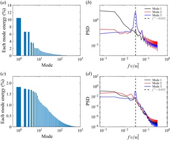
Appendix A. Proper orthogonal decomposition analysis
Energy proportion of each POD mode: (a) streamwise velocity fluctuation
 $u'$
; (c) wall-normal velocity fluctuation
 $v'$
. Power spectral density (PSD) of the first three POD expanded coefficients: (b) for
 $u'$
and (d) for
 $v'$
. Dashed lines in (b,d) mark the normalised frequency by the viscous time scale, i.e.
 $f^+=0.033$
, where
 $u'$
-modes 2 and 3 and
 $v'$
-mode 3 have their peaks.

Figure 15. Long description
Panel A: A vertical bar graph shows the energy proportion of each POD mode for streamwise velocity fluctuation. The x-axis is labeled ‘Mode’ and spans from 10^0 to 10^3. The y-axis is labeled ‘Each mode energy (%)’ and ranges from 0 to 14 percent. The bars decrease in height as the mode number increases. Panel B: A line graph displays the power spectral density (PSD) of the first three POD expanded coefficients for streamwise velocity fluctuation. The x-axis is labeled ‘fv/u_tau^2’ and ranges from 10^-3 to 10^0. The y-axis is labeled ‘PSD’ and ranges from 10^-5 to 10^0. Three lines represent different modes, with a dashed line marking a specific frequency. Panel C: A vertical bar graph shows the energy proportion of each POD mode for wall-normal velocity fluctuation. The x-axis is labeled ‘Mode’ and spans from 10^0 to 10^3. The y-axis is labeled ‘Each mode energy (%)’ and ranges from 0 to 2 percent. The bars decrease in height as the mode number increases. Panel D: A line graph displays the power spectral density (PSD) of the first three POD expanded coefficients for wall-normal velocity fluctuation. The x-axis is labeled ‘fv/u_tau^2’ and ranges from 10^-3 to 10^0. The y-axis is labeled ‘PSD’ and ranges from 10^-8 to 10^2. Three lines represent different modes, with a dashed line marking a specific frequency.
Following Meyer et al. (Reference Meyer, Pedersen and Özcan2007) and Borra et al. (Reference Borra, Flynn, Goza and Saxton-Fox2025), the POD analysis was performed as follows. The snapshot
 $\boldsymbol{u}=u'(x,z)$
was rearranged as an
 $I=N_x\times N_z$
column vector. We collect
 $N=1000$
such snapshots in time intervals of
 $0.003h/u_\tau$
and construct the matrix
 $\boldsymbol{U}$
as follows:
 \begin{equation} \boldsymbol{U} = \begin{bmatrix} \boldsymbol{u'}^1 & \boldsymbol{u'}^2 & \cdots & \boldsymbol{u'}^N \end{bmatrix}=\begin{bmatrix} u_1^{\prime 1} & u_1^{\prime 2} & \cdots & u_1^{\prime N} \\[5pt] \vdots & \vdots & \vdots & \vdots \\[5pt] u_I^{\prime 1} & u_I^{\prime 2} & \cdots & u_I^{\prime N} \end{bmatrix}\!. \end{equation}
The superscript
 $j=1,2,\dots , N$
indicates the number index of the snapshot. The objective of POD analysis is to find a hierarchical set of orthogonal modes to construct
 $\boldsymbol{U}$
. To accomplish this goal, the autocovariance matrix was created as
 \begin{equation} \widetilde {\boldsymbol{M}} = \boldsymbol{U}^T\boldsymbol{U}, \end{equation}
and then the eigenvalue problem for
 $\widetilde {\boldsymbol{M}}$
, i.e.
 \begin{equation} \widetilde {\boldsymbol{M}}\boldsymbol{V}^j=\lambda ^j\boldsymbol{V}^j, \end{equation}
was solved. As the kinetic energy of a POD mode is proportional to the magnitude of its eigenvalue, the eigenvalues were rearranged from largest to smallest, that is,
 \begin{equation} \lambda ^1\gt \lambda ^2\gt \lambda ^3\gt \cdots \gt \lambda ^N. \end{equation}
Next, the normalised POD modes
 $\boldsymbol{\phi }^j$
were constructed using the eigenvectors given by (A3), i.e.
 \begin{equation} \boldsymbol{\phi }^j = \frac {\sum _{n=1}^N V_n^j \boldsymbol{u'}^n}{\left |\right | \sum _{n=1}^N V_n^j \boldsymbol{u'}^n\left |\right |}, \quad \quad j=1,2,3,\dots ,N, \end{equation}
where
 $V_n^j$
is the
 $n$
th component of the eigenvector
 $\boldsymbol{V}^j$
with eigenvalue
 $\lambda ^j$
, and
 $||\boldsymbol{y}||=\sqrt {y_1^2+y_2^2+y_3^2+\cdots +y_I^2}$
is the
 $L_2$
norm of the vector
 $\boldsymbol{y}$
. Because
 $\boldsymbol{\phi }^j$
form a complete orthogonal basis,
 $\boldsymbol{u^{\prime n}}$
can be expanded based on POD modes:
 \begin{equation} \boldsymbol{u'}^n = \sum _{i=1}^N c_{\!j}^n\boldsymbol{\phi }^j = \boldsymbol{\varPhi }\boldsymbol{c}^n \end{equation}
and the corresponding coefficients
 $\boldsymbol{c}^n$
are
 \begin{equation} \boldsymbol{c}^n = \boldsymbol{\varPhi }^T\boldsymbol{u'}^n, \end{equation}
where
 $\boldsymbol{\varPhi } = [\boldsymbol{\phi }^1\quad \boldsymbol{\phi }^2\quad \boldsymbol{\phi }^3 \cdots \boldsymbol{\phi }^N]$
.
The percentage of kinetic energy contained in each mode was calculated as
 $\lambda _i/\sum _{n=1}^N\lambda _n$
, as shown in figure 15(a) for
 $\boldsymbol{u'}$
. Mode 1 contributes about 11 % to the total kinetic energy, while modes 2 and 3 contribute similar amounts of 7 %; the remaining modes each contribute less than 4 % to the total kinetic energy. The power spectral densities of the temporal coefficients
 $\boldsymbol{c}^n$
for the first three modes (
 $n=1, 2, 3$
) are shown in figure 15(b). The first mode corresponds to the merged streak envelope (figure 12
a), and the second and third modes correspond to the streamwise belt structures (figure 12
b,c), both taking a maximum at a frequency of
 $f^+=0.033$
. The latter indicates a viscous time scale of
 $T^+=1/f^+\approx 30$
for the dynamical period of the belt structures.
Similar POD analysis was performed for
 $\boldsymbol{v'}$
, as shown in figure 15(c) for the energy contribution and figure 15(d) for the power spectral density. The first seven modes of
 $v'$
make similar contributions to the total kinetic energy, each less than 2 %. The power spectral density of mode 3 exhibits a peak at a frequency of
 $f^+=0.033$
, indicating the same period of
 $30\nu /u^2_\tau$
as for
 $u'$
. This coincidence indicates that all the belt structures observed in figures 12(b), 12(c) and 12( f) have the same dynamical property.


 R
 N

 R
 As+−yc+
 Reτ=180
 Reτ=395
 Reτ=550
 ∙
 +
 R
 Reτ

 Reτ=550
 +
 #

 Reτ=550
 ⟨u′u′⟩+
 ⟨v′v′⟩+
 ⟨|u′v′|⟩+
 ⟨w′w′⟩+

 kzΦuu(y+,kz+)/uτ2
 kzΦuv(y+,kz+)/uτ2
 kzΦu~u~(y+,kz+)/uτ2
 kzΦu~v~(y+,kz+)/uτ2

 τw
 Reτ=180
 395
 550

 λ2
 y+=15
 Reτ=550

 λ2
 Reτ=550

 Reτ=550

 Reτ=180
 Reτ=395
 Reτ=550
 kx+=0.026

 y+=5
 y+=15
 y+=25
 v+
 w+
 u+
 z+=0

 x
 z
 y+=5
 Reτ=550

 CΩ
 TZ+TY
 TZ−R, TZ−C, TY−R, TY−C
 Cf,0

 y
 z
 u′
 v′
 u′
 v′
 f+=0.033
 u′
 v′


