1 Introduction
This work considers the flow of a suspension through a bifurcating channel. Flows of liquids containing dispersed solids through networks of channels or tubes are important in engineering and biomedical fields. As an example, hydraulic fracturing is a method to improve the rate of production of petroleum wells by inducing fractures in a crude oil- and natural gas-bearing geological formation and then pumping in a slurry of sand or engineered particles to prop open the fracture (Kulkarni et al. Reference Kulkarni, Manoorkar, Morris and Tonmukayakul2016). This leads to the name proppant for the solids (Warpinski et al. Reference Warpinski, Mayerhofer, Vincet, Cipolla and Lolon2009; Garagash & Lecampion Reference Garagash and Lecampion2014; Garagash, Lecampion & Desroches Reference Garagash, Lecampion and Desroches2015). In a different context, blood is largely a suspension of red blood cells in plasma, and the distribution of blood components in the branching arterial network is readily appreciated to have health-related implications (Pries et al. Reference Pries, Secomb, Gaehtgens and Gross1990; Pedley Reference Pedley2008). Flow in bifurcating networks of channels represents a significant challenge to present ability to predict mixture flows. We investigate suspension flow in a single bifurcating square channel, indicated in figure 1, as this is a critical step toward prediction of network flows.
While it is not sufficiently simple to isolate a single phenomenon, flow through a bifurcation elucidates issues that must be resolved to allow prediction of suspension, or any multiphase mixture, flow. Full knowledge of a mixture flow requires tracking the distribution of components, represented for a monodisperse suspension by the solid volume fraction,
 $\unicode[STIX]{x1D719}$
, and accounting for the influence of the components on the rheological properties. We outline these issues to indicate the fundamental motivations for this work, and its contributions. The bifurcation generates a flow where inertial effects play a pronounced role in the partitioning of single-phase Newtonian fluid to the two downstream branches, as the straight branch is increasingly the preferred path for the fluid with increasing
 $Re$
. Information which is of most importance in multiphase flow at a bifurcation, for fundamental as well as pragmatic reasons, is the partitioning of the specific components to the downstream branches. This study has as its primary goal the determination of how the particles and fluid partition, or ‘split’, at the bifurcation as a result of the interaction of inertia and solid fraction. The scope of our study is wide, as we consider
 $10<Re\leqslant 870$
, and pure fluid as well as suspensions of
 $0<\unicode[STIX]{x1D719}\leqslant 0.3$
. This allows consideration of the migration caused by particle-scale inertia as well as suspension rheology. Non-uniformity of
 $\unicode[STIX]{x1D719}$
over the channel cross-section caused by the migration is particularly influential in determining partitioning at a bifurcation. We show that a seemingly complex dependence on
 $Re$
of partitioning of the particles in the dilute suspension can be readily understood at a semi-quantitative level through combination of the results of separate analyses of (i) migration in pressure-driven suspension flow in straight channels and (ii) pure fluid flow in the bifurcation. However, this decoupled approach breaks down at elevated concentrations, at least partially as the result of particulate effects on the rheology: partitioning which leads to a higher solid fraction in the straight branch results in a higher effective viscosity and thus an increased wall shear stress at a given flux in this branch. As a consequence, for the larger
 $\unicode[STIX]{x1D719}$
studied, the side branch has higher flux, in stark contrast to the prediction of an effective fluid model in which uniform concentration is assumed, as this would yield the result for the single-phase fluid. Thus, the upstream migration is found to be coupled to the downstream hydraulic relation of axial flux to pressure gradient. Beyond its characterization of the basic dependence of the bifurcation flow of a suspension, this work provides guidance for a range of questions whose resolution is needed in order to advance predictive understanding in mixture fluid mechanics.
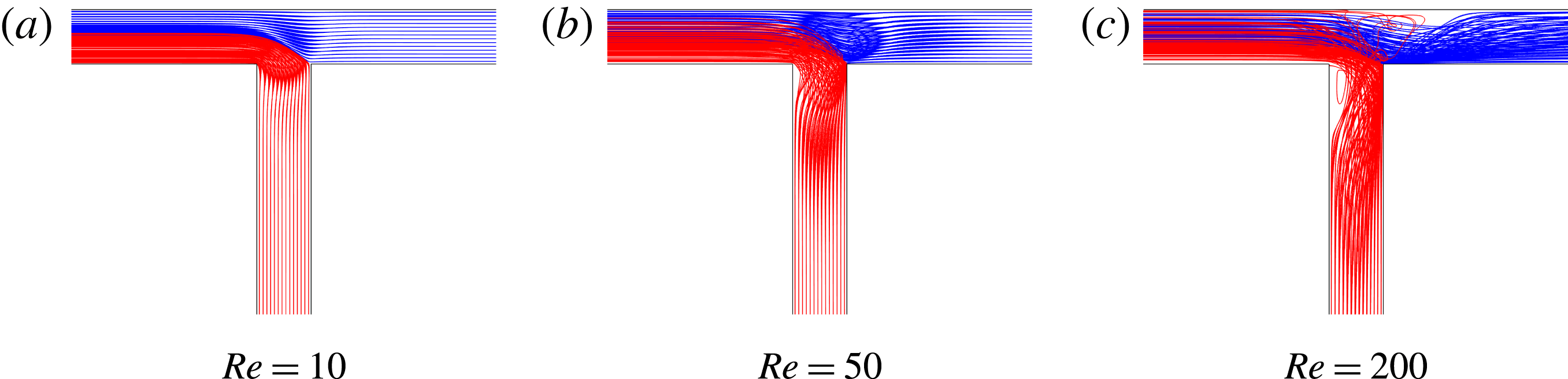
Streamlines obtained from COMSOL simulations of the pure fluid in the square cross-section T-channel. Flow enters at the upper left in each case, divides at the bifurcation and exits from the other two branches.

In particulate flows, different phenomena may be relevant depending on the solid fraction, and some delineation of regimes is useful. One can divide the phenomena into those of dilute suspensions where the single body motion at finite particle-scale inertia (non-zero particle-scale Reynolds number) is dominant, and those of concentrated suspensions where rheological phenomena are dominant, as developed in Guazzelli & Morris (Reference Guazzelli and Morris2012). This is by no means a strict division, as there clearly can be an interaction of inertia and rheology. We consider first the high volume fraction case. For this condition, bulk rheological properties of suspensions at vanishing
 $Re$
have been the topic of investigation for over a century (Einstein Reference Einstein1906; Roscoe Reference Roscoe1952), with early work focusing on the increase of effective suspension viscosity with solid volume fraction
 $\unicode[STIX]{x1D719}$
. The effective viscosity
 $\unicode[STIX]{x1D702}_{s}(\unicode[STIX]{x1D719})$
of the bulk suspension is often given as the ratio to the suspending fluid viscosity or the ‘relative viscosity’
 $\unicode[STIX]{x1D702}_{r}=\unicode[STIX]{x1D702}_{s}(\unicode[STIX]{x1D719})/\unicode[STIX]{x1D702}_{0}$
. This is given satisfactorily by a form diverging at a maximum packing fraction
 $\unicode[STIX]{x1D719}_{\mathit{max}}$
,
 $\unicode[STIX]{x1D702}_{r}=(1-\unicode[STIX]{x1D719}/\unicode[STIX]{x1D719}_{\mathit{max}})^{-1.82}$
(Krieger Reference Krieger1972), and other empirical forms also fit the behaviour well (Zarraga, Hill & Leighton Reference Zarraga, Hill and Leighton2000).
Suspensions at large solid loading also exhibit normal stress responses, including normal stress differences and a non-equilibrium osmotic pressure (or ‘particle pressure’) (Morris & Boulay Reference Morris and Boulay1999; Zarraga et al. Reference Zarraga, Hill and Leighton2000; Deboeuf et al. Reference Deboeuf, Gauthier, Martin, Yurkovetsky and Morris2009). Under low Reynolds number conditions, the normal stress is associated with breaking of microstructural isotropy (Morris Reference Morris2009). Of particular interest is the phenomenon of shear-induced migration (Koh, Hookham & Leal Reference Koh, Hookham and Leal1994; Hampton et al. Reference Hampton, Mammoli, Graham, Tetlow and Altobelli1997), which has been related to suspension normal stress (Shen et al. Reference Shen, Satake, Mehrabadi, Chang and Campbell1992; Nott & Brady Reference Nott and Brady1994; Morris & Boulay Reference Morris and Boulay1999; Boyer, Pouliquen & Guazzelli Reference Boyer, Pouliquen and Guazzelli2011). Particle migration leads to a non-uniform distribution of the particles in spatially varying shear flows and thus has a significant role in the flows described in this work.
In addition to migration which is associated with rheology in more concentrated suspensions, isolated particles migrate across the streamlines as a result of inertia. This migration was first observed as an accumulation or ‘pinching’ of particles at roughly 0.6 of the radius from the centreline in circular pipe flow of a dilute suspension by Segré & Silberberg (Reference Segré and Silberberg1961), followed by many other studies in pipe (Han et al.
Reference Han, Kim, Kim and Lee1999; Matas, Morris & Guazzelli Reference Matas, Morris and Guazzelli2004) and channel (Chun & Ladd Reference Chun and Ladd2006; Bhagat, Kuntaegowdanahalli & Papautsky Reference Bhagat, Kuntaegowdanahalli and Papautsky2008) geometries. The basis for inertial particle migration was analytically addressed by Rubinow & Keller (Reference Rubinow and Keller1961) and Saffman (Reference Saffman1965). The preferred or ‘equilibrium’ positions seen in the work of Segré & Silberberg were first analytically determined by Ho & Leal (Reference Ho and Leal1974) for a channel geometry. Later extensions of this theory considered higher
 $Re$
, which causes a closer approach to the boundary, for the channel (Schonberg & Hinch Reference Schonberg and Hinch1989; Asmolov Reference Asmolov1999) and the circular pipe (Matas, Morris & Guazzelli Reference Matas, Morris and Guazzelli2009). Han et al. (Reference Han, Kim, Kim and Lee1999) found that inertial migration is dominant for particle loadings of
 $\unicode[STIX]{x1D719}\leqslant 0.1$
, while at larger fractions inertial and rheological migration must both be considered to rationalize the particle distribution in the cross-section of a circular pipe. Of particular relevance here is experimental work by Miura, Itano & Sugihara-Seki (Reference Miura, Itano and Sugihara-Seki2014), which considered the migration of dilute particles at
 $\unicode[STIX]{x1D719}=O(10^{-4})$
in a square channel of side length 9.2 times the particle diameter at several axial distances and
 $100\leqslant Re\leqslant 1200$
.
The coupling between the upstream concentration profile and the dividing streamline for suspension flow at a bifurcation was considered by Yan, Acrivos & Weinbaum (Reference Yan, Acrivos and Weinbaum1991) to analyse ‘fluid skimming’ and particle entrainment into a small side pore at small
 $Re$
. Enden & Popel (Reference Enden and Popel1994) calculated the shape of the dividing streamline at the T-shaped bifurcation of two cylindrical tubes, also at low
 $Re$
, by a finite element method. In both of these studies, the authors considered a simple particle concentration profile by assuming a particle-free layer near the wall and an otherwise uniform concentration of particles. They superimposed this profile with their dividing streamline calculations to predict the downstream distribution of particles. The basic flow structure is critical to this process. For the conditions of interest here, streamlines and separation zones in the T-geometry for a pure fluid are shown in figure 1. For
 $Re=10$
, the flow does not separate, as shown by figure 1(a). A first separation zone, at the corner leading into the side channel, is visible in figure 1(b), at
 $Re=50$
. At
 $Re=200$
, a second separation zone along the wall opposite the side channel is observed, as shown by figure 1(c). Iwanami & Suu (Reference Iwanami and Suu1969) noted the two separation zones; the first to appear at the corner is rather standard, while that on the opposite wall is discussed in Pedley (Reference Pedley2008). The streamlines shown are projected from various planes normal to the viewing direction, and from figure 1(c), it is clear that significant three-dimensional flow takes place near the separation zones. Similar streamline structures have been considered in some detail by Neary & Sotiropoulos (Reference Neary and Sotiropoulos1996), whose numerical work compares well with experiments of Liepsch & Moravec (Reference Liepsch and Moravec1982).
There is a limited body of literature which addresses suspension flow in bifurcations. Early work of Bugliarello & Hsiao (Reference Bugliarello and Hsiao1964) described the solid fraction in the outlet branches for several inlet solid concentrations, for imposed flow rate ratios in the downstream branches; this is similar to the present work, but we fix the pressure drop in the outlet branches and determine the flow rates. In studies at small
 $Re$
, Roberts & Olbricht (Reference Roberts and Olbricht2006) studied suspension flow in different bifurcations as a separation technique, while Xi & Shapley (Reference Xi and Shapley2008) measured the velocity and concentration profiles in an asymmetric bifurcation by using nuclear magnetic resonance imaging; similar geometries and conditions have been modelled by Ahmed & Singh (Reference Ahmed and Singh2011). Understanding the behaviour of the blood circulatory network was noted as a motivation above, and in this direction, Pries et al. (Reference Pries, Secomb, Gaehtgens and Gross1990) simulated flow through large circulatory networks using a viscosity model; this is a limited approach as it is known that the concentration of red blood cells is higher in the branch with higher volumetric flow rate, a phenomenon known as the Zweifach–Fung effect and shown to involve the particle deformation by Doyeux et al. (Reference Doyeux, Podgorski, Peponas, Ismail and Coupier2011).
As the flow problem of a mixture in a bifurcation is complex, added complications due to deformation or due to differences in density between particles and fluid (and associated rising and settling) are not considered here. We seek to establish the behaviour of rigid particle suspensions in a right angle bifurcation as a function of the Reynolds number and solid fraction
 $\unicode[STIX]{x1D719}$
. The Reynolds number is defined as
 $Re=(\unicode[STIX]{x1D70C}DU)/\unicode[STIX]{x1D702}$
;
 $U$
is the average axial velocity in the inlet branch of diameter
 $D$
, while
 $\unicode[STIX]{x1D70C}$
and
 $\unicode[STIX]{x1D702}$
are the fluid density and viscosity, respectively. We have examined both single-phase Newtonian fluid and suspension flows at a range of particle volume fractions
 $\unicode[STIX]{x1D719}$
through the asymmetric T-geometry illustrated by figure 1. We consider
 $Re=O(10)-O(1000)$
, so that the flow of the pure fluid is laminar but becomes strongly affected by inertia, with the noted separation zones appearing for larger
 $Re$
at the corner entering the side branch (figure 1
b) and on the opposite wall (figure 1
c). The studies involve extensive experiments and calculations by a combination of numerical methods. The latter include standard calculations for the pure fluid, lattice-Boltzmann method calculations for discrete-particle motion and migration in straight channels, and an advanced immersed boundary method for computing the discrete-particle flow at elevated Reynolds number through a bifurcating channel. This provides an unprecedented level of detail in the description of this flow, and provides guidance toward the more basic phenomena giving rise to the complex distribution of the phases in the two downstream branches.
The experimental and numerical methods are described in §§ 2 and 3, respectively. Results of the experiments and comparison with numerical calculations are presented in § 4. A detailed examination of flow structures and particle distribution from computation is presented in §§ 4.2 and 4.3, followed by concluding remarks.
2 Experiment
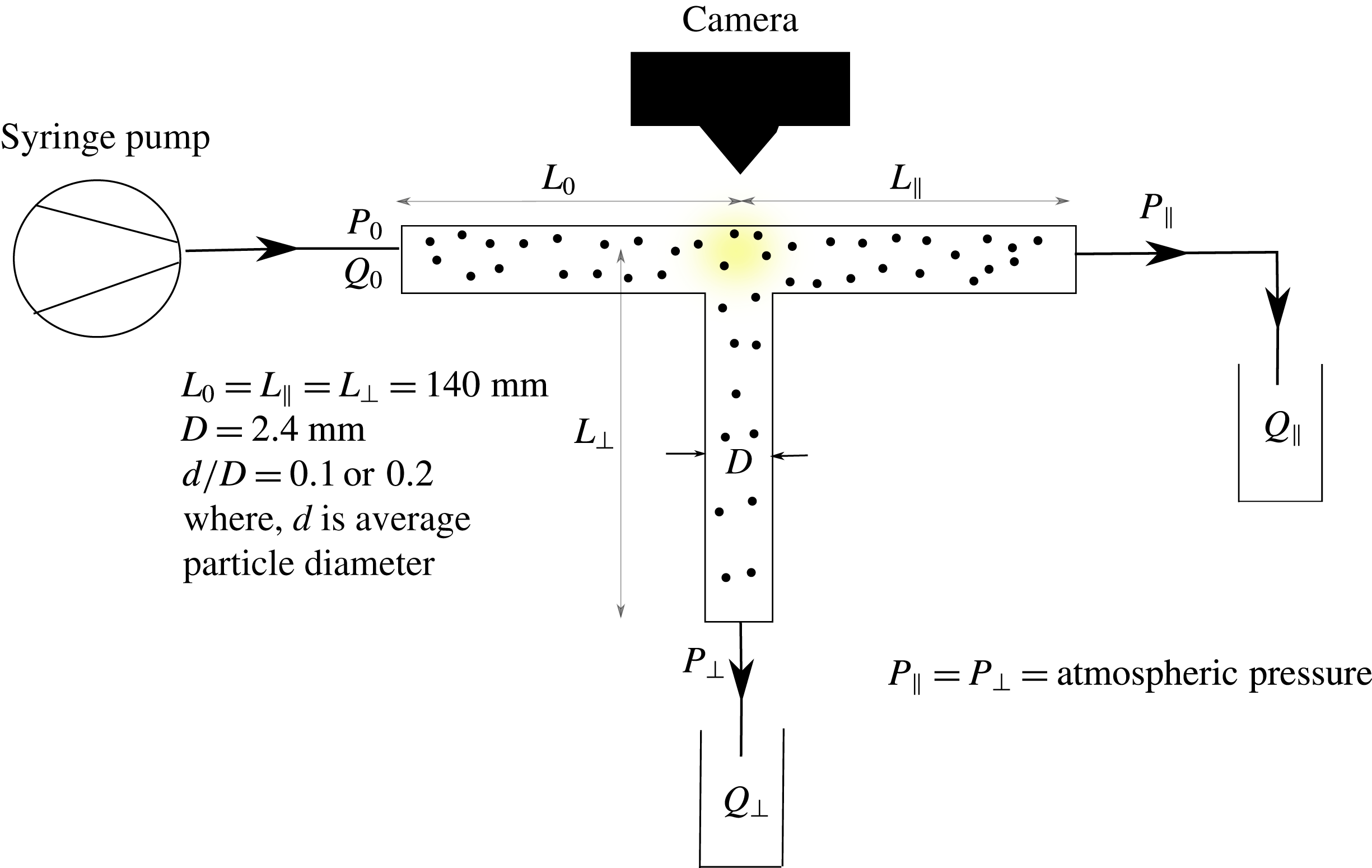
The experimental device is fabricated using two acrylic sheets where the T-shaped channel is etched in one of the sheets, and the other sheet is affixed to the top of the etched sheet to form a fully bounded channel of square cross-section, with the side length of
 $D=2.4~\text{mm}$
. Entry and exit ports to the channel at the boundary of the sheet are each 140 mm from the midpoint of the T-junction, so that
 $L_{\Vert }=L_{\bot }=L_{0}=140~\text{mm}$
, yielding the channel aspect ratio
 $L_{0}/D=58$
. A schematic of the experimental set-up is given in figure 2. Flow is driven by a syringe pump (Harvard Apparatus PhD 2000). High-speed cameras (Photron FASTCAM 1024 PCI) are mounted at the junction, one vertically and a second providing a perpendicular view for stereo imaging (not used in the work presented here).
The channels were tested to determine that very nearly the same flow resistance was present in each of the two outlet branches. The ratio of flux through the straight outlet branch to the inlet flux is defined as
 $\unicode[STIX]{x1D6FD}=Q_{\Vert }/Q_{0}$
, and this is subscripted in the case of suspension flow to describe the flux ratio for the bulk suspension or the individual (fluid and particle) components. Equality of resistance was determined by considering the pure fluid flow in the limit of small Reynolds number, where the ratio
 $\unicode[STIX]{x1D6FD}\doteq 0.5$
should be found based on Stokes-flow calculations. To within a small experimental uncertainty, the channels used yield
 $\unicode[STIX]{x1D6FD}=0.5$
for
 $Re\rightarrow 0$
, as will be shown below.
Schematic of experimental set-up.

The suspensions were prepared using spherical polystyrene particles (density
 $\unicode[STIX]{x1D70C}_{p}=1.051~\text{g}~\text{cm}^{-3}$
) in two size ranges (
 $150{-}360~\unicode[STIX]{x03BC}\text{m}$
with mean diameter
 $250~\unicode[STIX]{x03BC}\text{m}$
(standard deviation
 ${\approx}40~\unicode[STIX]{x03BC}\text{m}$
) and
 $360{-}610~\unicode[STIX]{x03BC}\text{m}$
with mean
 $480~\unicode[STIX]{x03BC}\text{m}$
(standard deviation
 ${\approx}35~\unicode[STIX]{x03BC}\text{m}$
); Maxi-Blast Inc.) and a density-matching water–glycerol mixture. The majority of the experiments were performed using the smaller particles, for which
 $d/D\approx 0.1$
. The dynamic viscosity of the water–glycerol mixture (
 $17\,\%$
glycerol and
 $83\,\%$
water, by volume) matching the density of the polystyrene particles is
 $\unicode[STIX]{x1D702}=0.0016\pm 0.00005$
Pa s at
 $25\,^{\circ }\text{C}$
.
The fluid is pumped through the channel at varying flow rates to obtain a wide range of Reynolds number, defined in terms of the flow rate in the inlet branch. The typical range of average velocity in the channel is
 $0.01{-}0.58~\text{m}~\text{s}^{-1}$
which corresponds to
 $17\leqslant Re\leqslant 870$
. The two outlets of the channel are open to atmospheric pressure. In each experiment, 30 ml of the fluid or suspension under study is pumped through the inlet and is collected from the outlets. For every inlet Reynolds number studied, five replicate experiments are performed with the same fluid mixture to achieve statistically significant results; note that the channel was full with the suspension before beginning collection of samples at the outlets, and to study whether this had an effect, larger volumes of fluid were collected for the test runs (50 and 60 ml), with no difference in the measured partitioning.
We determine
 $\unicode[STIX]{x1D6FD}_{\mathit{suspension}}$
as the ratio of suspension weight captured at the outlet of the straight branch to inlet branch. The suspensions are then filtered to separate the particles, and the particles obtained from each sample are dried at
 $80~^{\circ }\text{C}$
for several hours in an oven and weighed, with the ratio of the mass of the particles in the straight branch to the total flowing through the inlet branch giving
 $\unicode[STIX]{x1D6FD}_{\text{particle}}$
. By difference from the total suspension, one can calculate
 $\unicode[STIX]{x1D6FD}_{\mathit{fluid}}$
; we present both in some cases for ease of understanding. In addition to these gravimetric measurements, images are captured at 2000 fps at the bifurcation zone with the resolution of
 $1024\times 512\text{ pixels}$
over a region of
 $1.5\times 0.75~\text{cm}$
.
3 Numerical studies
3.1 Single-phase flow
The pressure-driven flow of a Newtonian fluid in the T-geometry was computed using a commercial solver (COMSOL). The computational domain was defined to match the geometric parameters of the experimental apparatus, defining
 $L_{0}=L_{\Vert }=L_{\bot }=1$
and
 $L_{0}/D=58$
. The incompressible Navier–Stokes equations were solved in this computational domain, with the fully developed laminar flow at the inlet and the same reference pressure at each outlet, along with no-slip boundary condition at the channel walls. Various computational meshes were used to establish mesh independence, with the finest mesh consisting of approximately
 $5.9\times 10^{5}$
hexahedral elements.
The computations were performed at inlet Reynolds numbers of
 $10<Re<700$
. The computed flow split to the downstream branches as a function of
 $Re$
was found to closely match the experimental results for the pure fluid. The simulation results were also used to investigate the detailed flow structure in the bifurcation region. The qualitative flow features, such as the complex three-dimensional streamline structure (as shown in figure 1
c), have been reported in the literature (Neary & Sotiropoulos Reference Neary and Sotiropoulos1996).
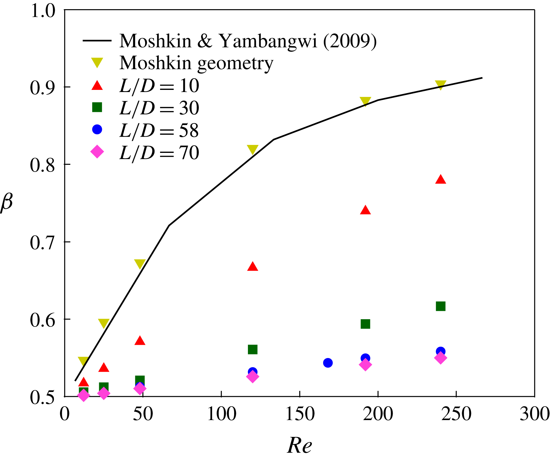
Figure 3 shows the numerically determined fractional flow in the straight branch,
 $\unicode[STIX]{x1D6FD}=Q_{\Vert }/Q_{0}$
, for
 $Re<300$
at various
 $L/D$
. This serves as a validation test of the numerical method, with the simulations performed for a T-channel having dimensions
 $L_{0}/D=2.5$
and
 $L_{\Vert }/D=L_{\bot }/D=3.5$
. This geometry corresponds to that used in a study by Moshkin & Yambangwi (Reference Moshkin and Yambangwi2009). The value of
 $\unicode[STIX]{x1D6FD}$
does not depend on
 $L_{0}$
in our calculation, as the steady laminar flow is enforced at the inlet, but is significantly influenced by the outlet lengths
 $L_{\Vert }$
and
 $L_{\bot }$
: this dependence is caused by the separation zones in the downstream branches which are disturbed when the outlet length is too short. As an example, if the side outlet length is very short, the separation zone which occurs at the sharp corner leading into the side branch does not develop fully. For sufficient outlet lengths, only small effects are seen with further increase of
 $L/D$
, as shown in figure 3:
 $L/D=58$
and
 $L/D=70$
have similar
 $\unicode[STIX]{x1D6FD}$
over all
 $Re$
studied.
Numerical results for the flow split
 $Q_{\Vert }/Q_{0}$
at different
 $L_{0}/D$
, where
 $L_{0}=L_{\Vert }=L_{\bot }=L$
.

3.2 Lattice-Boltzmann method: analysis of migration
The lattice-Boltzmann method (LBM) for particulate suspensions was used to simulate the pressure-driven flow of a dilute (
 $\unicode[STIX]{x1D719}_{0}=0.05$
) suspension through a channel of square cross-section. The LBM for suspensions is a fully coupled multiphase approach where the fluid phase dynamics is modelled using a discretized Boltzmann equation, and the particles are represented as hard spheres obeying Newtonian mechanics (Ladd Reference Ladd1994a
,Reference Ladd
b
; Aidun, Lu & Ding Reference Aidun, Lu and Ding1998; Haddadi & Morris Reference Haddadi and Morris2014). Full details of the method can be found in the noted references, while application to pressure-driven flow is described in Haddadi, Shojaei-Zadeh & Morris (Reference Haddadi, Shojaei-Zadeh and Morris2016). Close particle interactions are handled using the lubrication method described in Nguyen & Ladd (Reference Nguyen and Ladd2002), and the simulation is stopped if overlap is detected (as this demands careful consideration of solid collisions, which are out of scope for this work); collisions were not observed for the straight channel simulations reported using the LBM in this study.
The goal of these calculations was to determine the particle distribution in the cross-section resulting from inertial migration in the inlet branch. This was considered for smaller particles only for a dilute suspension. We simulated the pressure-driven flow of a suspension of
 $\unicode[STIX]{x1D719}_{0}=0.05$
in a straight channel with a square cross-section,
 $d/D=0.134$
at a range of
 $Re$
. The cross-sectional (
 $y$
–
 $z$
) positions of the particles were recorded as the flow progressed, and we have used here the values when the mean axial (
 $x$
) dimensionless distance travelled was equivalent to
 $L_{0}/D$
for the experimental inlet section. To analyse the influence of particle migration on
 $\unicode[STIX]{x1D6FD}$
, the flow split parameter, these particle profiles were then superimposed with the cross-sectional pure fluid streamline data in the T-junction calculated at the same
 $Re$
. Assuming particles at a position in the cross-section just before the bifurcation follow the fluid streamline which would otherwise pass through their centre, we obtain an estimate of the particle split: this is given by the flux ratio for particles on streamlines following the straight channel relative to those on streamlines which are diverted to the side branch, and thus requires considering the velocity of the streamlines on which each particle resides. Similar calculations to address migration have also been performed for
 $d/D=0.2$
for several volume fractions and these are reported below.
3.3 Immersed boundary method for discrete particles
The immersed boundary method (IBM) is a generic term for methods that simulate flows with embedded boundaries on grids that do not conform to the shape of these boundaries (Mittal & Iaccarino Reference Mittal and Iaccarino2005). The key idea behind IBM is to use a fixed mesh (Eulerian mesh or grid) for the computation and represent the immersed object using a different mesh (Lagrangian mesh), which is free to move over the domain of the fixed mesh. Such methods have been used to simulate a variety of particle-laden flows (Kempe & Fröhlich Reference Kempe and Fröhlich2012b ; Lashgari et al. Reference Lashgari, Picano, Breugem and Brandt2016).
The IBM solver used here is implemented in CDP, a massively parallel, unstructured finite-volume fluid solver developed at Stanford University’s Center for Turbulence Research (Ham, Mattsson & Iaccarino Reference Ham, Mattsson and Iaccarino2006; Ham Reference Ham2007). The idea behind the method is to extend the flow equations over the entire domain including the particle regions, which are assumed to be filled with fluid of density equal to the particles. The fluid in the volume occupied by particles is constrained to rigid body motion by adding an additional body force term in the momentum conservation equations.
The numerical algorithm is briefly described. In the first step, we solve the Navier–Stokes equations without additional constraint forces; we solve the momentum equations, without consideration of mass conservation. The solution in terms of the velocity field inside the particle domain, which is obtained by interpolation from the Eulerian mesh, is then projected onto a rigid body motion. This is accomplished by computing the translational and rotational components of the rigid body motion using the statement of conservation of linear and angular momentum. From the rigid body motion, we can evaluate the rigidity constraint force (the immersed boundary forcing), which is applied as a correction to the velocity field on the Eulerian mesh, together with the usual constraint of zero velocity divergence to enforce mass conservation. Finally, using the particle velocities, we update their positions. Since the grid sizes do not allow resolution of lubrication forces, we also employ a collision model to treat particle–particle and particle–wall interactions (Glowinski et al.
Reference Glowinski, Pan, Hesla, Joseph and Periaux2001; Kempe & Fröhlich Reference Kempe and Fröhlich2012a
). Collisions are of minimal influence on the results here. While collisions may be expected to be of greater influence at high solid fractions, here we only consider the
 $\unicode[STIX]{x1D719}_{0}=0.05$
case, for which local concentrations reaching as high as 15–20 % solids at full development are found in the LBM simulations. Further details of the algorithm along with the verification and validation of the IBM solver on unstructured grids can be found in Krishnan, Shaqfeh & Iaccarino (Reference Krishnan, Shaqfeh and Iaccarino2017).
The goal of the IBM simulations here was to simulate suspension flows in geometries similar to that of the experiment, compare the predictions and study the particle distributions. Unlike typical immersed boundary studies, which use structured Cartesian grid-based algorithms, the unstructured grid IBM solver is efficient for representation of geometries such as the T-junction (Krishnan et al.
Reference Krishnan, Shaqfeh and Iaccarino2017). Simulations are carried out for a suspension of concentration
 $\unicode[STIX]{x1D719}_{0}=0.05$
with the particle sizes
 $d/D=0.1$
and 0.2 for
 $10\leqslant Re\leqslant 700$
.
For
 $d/D=0.2$
, the geometry used agreed with that of experiments (
 $L_{0}=L_{\Vert }=L_{\bot }=58D\approx 290d$
). The domain was discretized into uniform hexahedral elements of size
 $h=D/40$
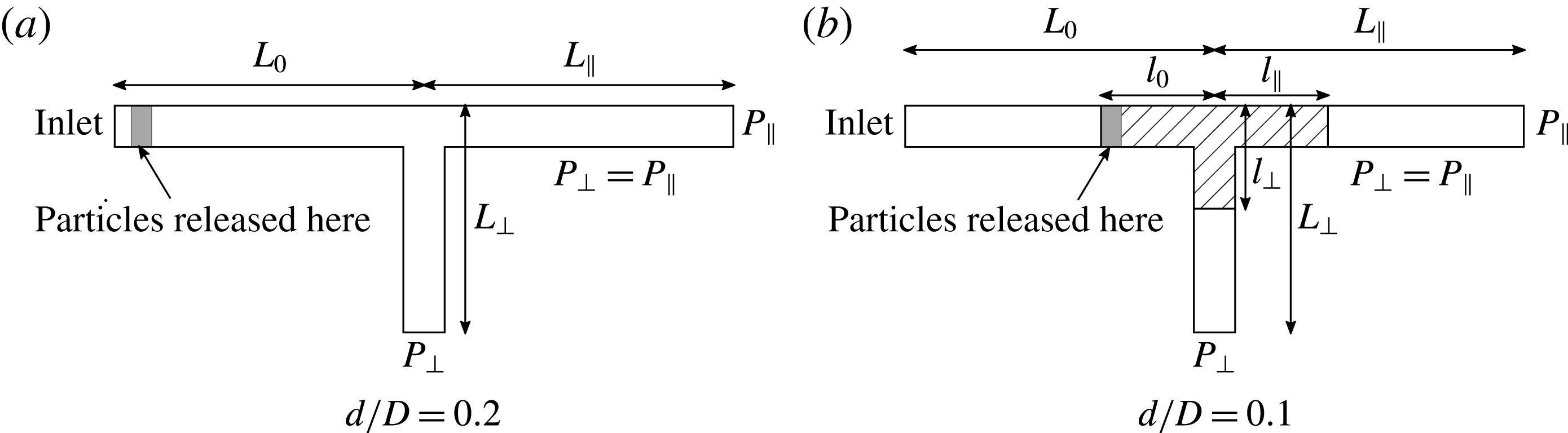
, resulting in a total of 11.3 million elements with eight Eulerian cells across the particle. A fully developed flow was specified at the inlet and the two outlets were maintained at the same pressure, below that at the inlet. After the flow reached steady state, neutrally buoyant particles were released close to the inlet (figure 4
a), at random from a uniform distribution across the inlet cross-section at a rate governed by the volume fraction
 $\unicode[STIX]{x1D719}$
. The simulations do not take into account the size distribution of the particles and the particle size in the simulation was set to the mean particle size in the experiments. Each simulation was continued until a statistically significant number, of
 $O(1000)$
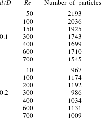
, of particles reached the bifurcation. The numbers of particles considered in the IB simulations were different for each (
 $Re$
,
 $d/D$
) pair and the values are given in table 1. The simulations were continued until the ratio
 $N_{\Vert }/N_{\bot }$
reached a steady state value, where
 $N_{\Vert }$
is the number of particles which crossed the junction into the straight outlet branch and
 $N_{\bot }$
is the number of particles which crossed the junction into the side outlet branch.
Numbers of particles used in IB simulations for each (
 $Re$
,
 $d/D$
) pair.

For
 $d/D=0.1$
, we used a smaller domain (
 $l_{0}=l_{\Vert }=l_{\bot }=7.25D=72.5d$
) where the particulate flow is computed, so that the total number of cells remain computationally tractable, while maintaining eight Eulerian cells across the particle, i.e.
 $h=D/80$
. This region is shown with diagonal lines in figure 4(b). The rest of the domain is discretized using
 $h=D/40$
resulting in a total of 22.3 million elements. In this case, however, we do not know the particle distribution across the cross-section of the release region. We make the approximation that the particle distribution at the inlet is the same as the steady state cross-sectional distribution of initially randomly distributed particles in a square channel flow of identical cross-section since both
 $L_{0}-l_{0}$
and
 $l_{0}$
are large relative to
 $d$
. We find this distribution by simulating at each
 $Re$
studied a suspension of
 $\unicode[STIX]{x1D719}_{0}=0.05$
in a square channel (periodic in the flow direction with a domain length of
 $100d$
) and the same cross-section as in the experiments.
Schematic for immersed boundary method simulations. In (a), the particles are released a few particle diameters away from the inlet so as to not affect the Dirichlet boundary conditions at the inlet. In (b), the particulate flow is computed only in the shaded region.

4 Results and discussion
4.1 Experiments
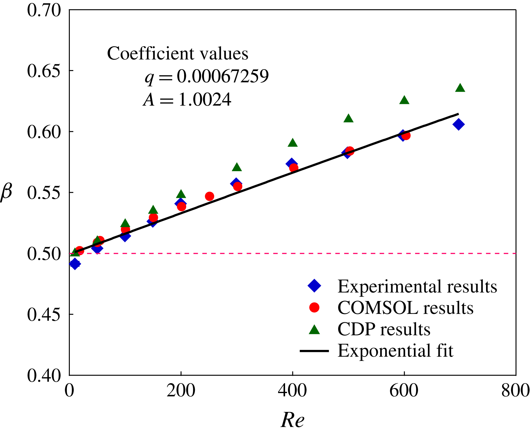
To establish the reliability of our experimental device, single-phase Newtonian flow was studied. Figure 5 shows the variation of the single-phase fractional flow rate into the straight outlet branch with the inlet channel Reynolds number, denoted
 $\unicode[STIX]{x1D6FD}(Re)$
. It should be noted that error bars based on the dispersion of the measurements at a nominal condition are plotted throughout, and are consistently small, in part because the measurements are from multiple replicate experiments using the same well-mixed sample at each condition. An intrinsic uncertainty in the concentration and in the exact geometry are not accounted for in these error bars. At low
 $Re$
,
 $\unicode[STIX]{x1D6FD}\approx 0.5$
. As
 $Re$
number increases,
 $\unicode[STIX]{x1D6FD}$
increases, with the dependence of the increase on
 $Re$
well fitted by
 $$\begin{eqnarray}\displaystyle & \unicode[STIX]{x1D6FD}={\displaystyle \frac{1}{1+A\text{e}^{-qRe}}}. & \displaystyle\end{eqnarray}$$
The two parameters of the fit are geometry specific, and for the equivalent outlet lengths and square channel sizes used here are given by
 $A=1$
and
 $q=6.72\times 10^{-4}$
. If the side channel were smaller, for example, one expects a smaller
 $A$
, while the details of
 $q$
will depend on the size and angle of the side channel relative to the straight channel. While this is an empirical fit, the value of
 $A$
can be rationalized. For sufficiently low
 $Re$
, when flow approaches the Stokes regime, streamlines divide equally at the junction to yield
 $\unicode[STIX]{x1D6FD}\doteq 0.5$
: there is negligible excess energy dissipated as a result of the flow bifurcation so that the flow is determined by the pressure drop across the two branches and these are equal. As
 $Re$
increases, streamlines near the centre of the channel become more difficult to divert, leading to an increasing
 $\unicode[STIX]{x1D6FD}$
. The exponential in the denominator of (4.1) results in the decay of the fluid flux diverted to the side channel, apparently due to the reduced time of exposure to the transverse pressure gradient as flow rate (and hence
 $Re$
) increases. Numerical calculation of
 $\unicode[STIX]{x1D6FD}$
by both COMSOL and CDP agrees well with the experiments, with CDP slightly over-predicting the experimental value of
 $\unicode[STIX]{x1D6FD}$
. The difference in flow rate between the numerical methods is approximately 3.5 % at the highest
 $Re$
and the values from CDP are expected to be the more reliable, as they are more highly resolved; the closer fit to the experiment from the COMSOL results is coincidental, as the experimental quality of the channels renders the experiment the most uncertain quantity plotted.
Experimental results for single-phase Newtonian fluid,
 $\unicode[STIX]{x1D719}_{0}=0$
.

In the small
 $Re$
range, the closeness to
 $\unicode[STIX]{x1D6FD}=0.5$
validates our experimental set-up, as it was found that even small imperfections of the device lead to substantial deviations from the value
 $\unicode[STIX]{x1D6FD}(Re\rightarrow 0)=0.5$
. Qualitatively these results are consistent with the numerical studies of Moshkin & Yambangwi (Reference Moshkin and Yambangwi2009), but quantitative differences are found owing to the short outlet lengths assumed in these earlier calculations.
Video information. To provide the most direct access to the behaviour at the bifurcation, videos captured from experiments are provided, and some of these are compared with videos of the immersed boundary simulations. These all show the flow of suspensions at
 $\unicode[STIX]{x1D719}=0.05$
and
 $d/D=0.2$
, and the noted size dispersion can be seen in the experimental videos. The videos are described in order of increasing
 $Re$
. Movies 1 and 2, available at https://doi.org/10.1017/jfm.2018.183, show experimental and immersed boundary simulation results at
 $Re=200$
, respectively. In movie 3, results of experiment and simulation are shown together, at
 $Re=300$
for simulations and
 $Re=311$
for experiments. Experimental video at
 $Re=415$
is shown in movie 4. A comparison is presented in movie 5, at
 $Re=600$
and 620 for simulations and experiments, respectively. Movie 6 shows the experimental behaviour at
 $Re=830$
. Note that movie 2 displays, for the simulations, the inlet and bifurcation regions in zoom form and the motion through the channel as it fills. In the bifurcation videos, particles are seen to be largely absent from the recirculating regions associated with flow separation, but occasionally particles are trapped and make numerous circuits, particularly at the higher
 $Re$
. Complex three-dimensional motions accompany trapping in the recirculation at the wall opposite the side channel, as there is a spiralling component to the recirculation, as indicated by figure 1(c), or the work of Neary & Sotiropoulos (Reference Neary and Sotiropoulos1996). As a consequence, particles may follow surprising trajectories, making several circuits downstream of the bifurcation and then exiting the recirculation near one wall (with normal along the viewing axis), to either branch. The experimental portion of the simultaneous experiment – simulation video at
 $Re\approx 600$
in movie 5 exhibits a number of such trajectories in which the particles move ‘upstream’ (against the mean flow) in the straight branch, with interactions with the axial stream causing fluctuating motion, and then depart to either the side channel or into the straight branch. When the exit is by the straight branch, particles typically closely approach the downstream corner. The motion of particles can be seen to lead to solid collision at this corner at all conditions presented in the videos, and there is good fidelity in replicating this phenomenon in the simulations. Analysis of the detailed motion of particles in the vicinity of the bifurcation using stereo imaging (two-camera view) is experimentally performed, but is out of scope for this study where flow partitioning is the focus.
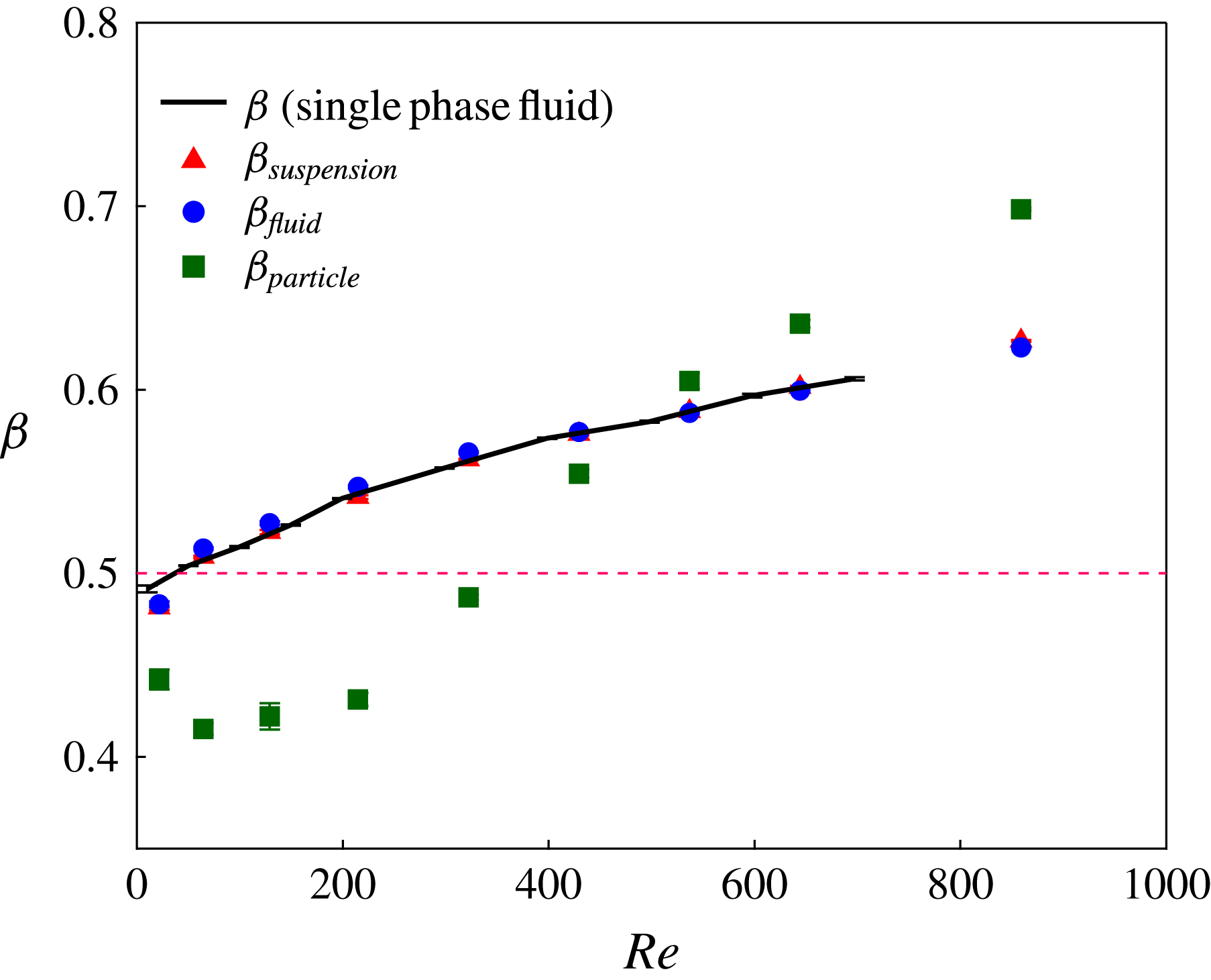
Figure 6 shows the flow ratios, or ‘splits’, measured experimentally for the suspension at
 $\unicode[STIX]{x1D719}_{0}=0.05$
. Here, we use
 $\unicode[STIX]{x1D6FD}$
to designate pure fluid data, plotted to provide a comparison with the bulk suspension and phase splits, which are denoted by subscripts. As expected, because the mixture is mostly the fluid,
 $\unicode[STIX]{x1D6FD}_{\mathit{suspension}}\approx 0.5$
at the lowest
 $Re=17$
and follows
 $\unicode[STIX]{x1D6FD}$
of the fluid as
 $Re$
increases. This indicates that the dividing streamlines of the mixture remain essentially the same as those of the pure fluid for this dilute suspension.
Experimental results for the flow ratios at
 $\unicode[STIX]{x1D719}_{0}=0.05$
as a function of
 $Re$
.

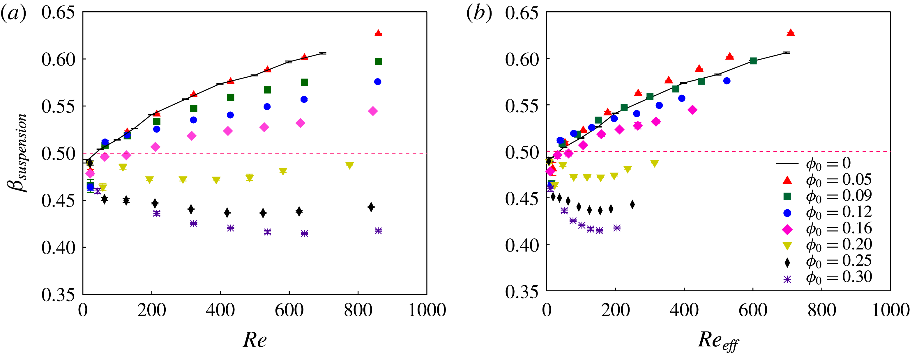
Suspension flow ratio for various inlet solid concentrations,
 $\unicode[STIX]{x1D719}_{0}$
: (a)
 $Re$
based on pure fluid viscosity and (b)
 $Re$
based on effective bulk suspension viscosity.

Figure 7 shows
 $\unicode[STIX]{x1D6FD}_{\mathit{suspension}}$
for several inlet particle volume fractions,
 $\unicode[STIX]{x1D719}_{0}$
. It is observed that
 $\unicode[STIX]{x1D6FD}_{\mathit{suspension}}\approx 0.5$
for the smallest
 $Re$
in all cases, but the dependence on
 $Re$
is qualitatively different depending upon
 $\unicode[STIX]{x1D719}_{0}$
. As
 $\unicode[STIX]{x1D719}_{0}$
increases, progressively less material flows to the straight branch, resulting in a lower
 $\unicode[STIX]{x1D6FD}_{\mathit{suspension}}$
for the same
 $Re$
as shown in figure 7(a); recall that here
 $Re$
is based on the pure fluid viscosity. For
 $0<\unicode[STIX]{x1D719}_{0}<0.20$
,
 $\unicode[STIX]{x1D6FD}_{\mathit{suspension}}$
increases with
 $Re$
. For
 $\unicode[STIX]{x1D719}_{0}>0.20$
, an initial decrease with
 $Re$
gives way to a slight increase as we approach the highest flow rates of
 $Re>800$
. We note that
 $\unicode[STIX]{x1D6FD}_{\mathit{suspension}}$
for
 $\unicode[STIX]{x1D719}_{0}\geqslant 0.20$
remains lower than
 $0.5$
for all
 $Re$
, implying that more material enters the side branch for every condition: this is a distinct contrast from the behaviour of the pure liquid for which
 $\unicode[STIX]{x1D6FD}>0.5$
and grows with
 $Re$
. To account for the added viscous dissipation due to the particles, we have also plotted, in figure 7(b),
 $\unicode[STIX]{x1D6FD}_{\mathit{suspension}}$
as a function of
 $Re_{\mathit{effective}}=Re/\unicode[STIX]{x1D702}_{r}$
, where the apparent viscosity is given by
 $\unicode[STIX]{x1D702}_{r}=(1-\unicode[STIX]{x1D719}/\unicode[STIX]{x1D719}_{\mathit{max}})^{-1.82}$
with
 $\unicode[STIX]{x1D719}_{\mathit{max}}=0.55$
. When effective viscosity is used in the Reynolds number, the
 $\unicode[STIX]{x1D719}_{0}=0.05$
data shift to smaller
 $Re_{\mathit{effective}}$
relative to the pure fluid, and this appears to be inconsistent; particle migration may result in this rescaling being inappropriate for small loadings.
Component splits in T-channel as a function of
 $Re$
for different inlet solid fractions,
 $\unicode[STIX]{x1D719}_{0}$
. (a) Fluid split and (b) particle split. This figure omits
 $\unicode[STIX]{x1D719}_{0}=0.05$
which is plotted in figure 6.

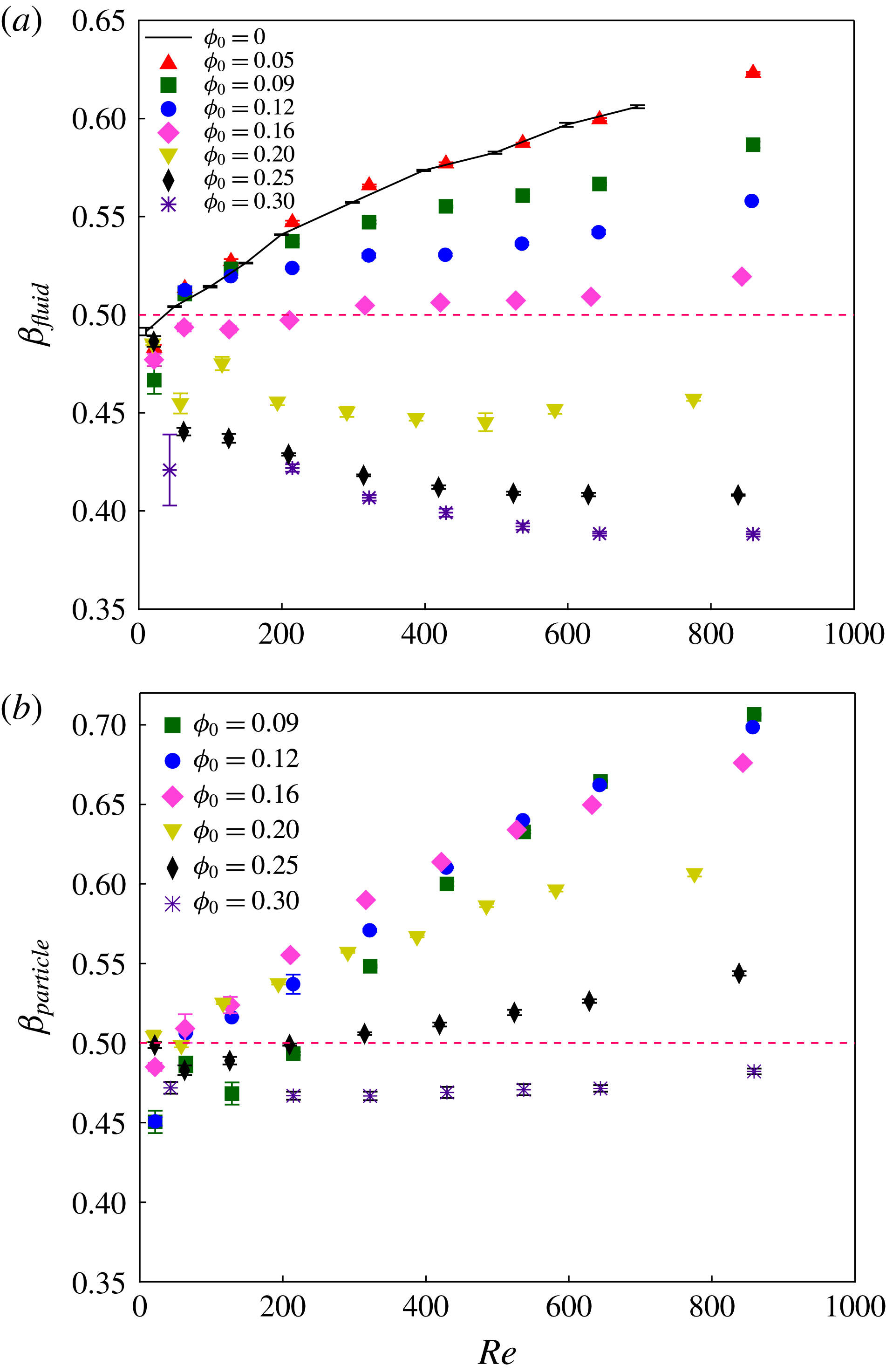
We consider next the individual component flow ratios. The ratio for the fluid,
 $\unicode[STIX]{x1D6FD}_{\mathit{fluid}}$
, is plotted as a function of
 $Re$
in figure 8(a), showing that fluid from the concentrated suspension is disproportionately diverted to the side channel, with
 $\unicode[STIX]{x1D6FD}_{\mathit{fluid}}<0.5$
for
 $\unicode[STIX]{x1D719}_{0}\geqslant 0.2$
. Noting that an effective viscosity calculation would simply shift the results horizontally to a smaller Reynolds number, as demonstrated by the rescaling in figure 7, this result demands a multiphase mixture explanation associated with the particle distribution in the cross-section as it enters the bifurcation. In figure 8(b),
 $\unicode[STIX]{x1D6FD}_{\mathit{particle}}$
is plotted against
 $Re$
, and the minimum seen for
 $\unicode[STIX]{x1D719}_{0}=0.05$
is not found at higher inlet solid fraction, except perhaps for a single value of
 $\unicode[STIX]{x1D6FD}_{\mathit{particle}}<0.5$
at the smallest
 $Re$
studied for
 $\unicode[STIX]{x1D719}_{0}=0.09$
. For larger
 $\unicode[STIX]{x1D719}_{0}$
,
 $\unicode[STIX]{x1D6FD}_{\mathit{particle}}$
increases with
 $Re$
for
 $\unicode[STIX]{x1D719}_{0}<0.25$
. However, for the highest solid loading studied,
 $\unicode[STIX]{x1D719}_{0}=0.30$
, more particles go to the side channel, giving
 $\unicode[STIX]{x1D6FD}_{\mathit{particle}}<0.5$
and its value remains almost constant at
 $\unicode[STIX]{x1D6FD}_{\mathit{particle}}\approx 0.47$
.
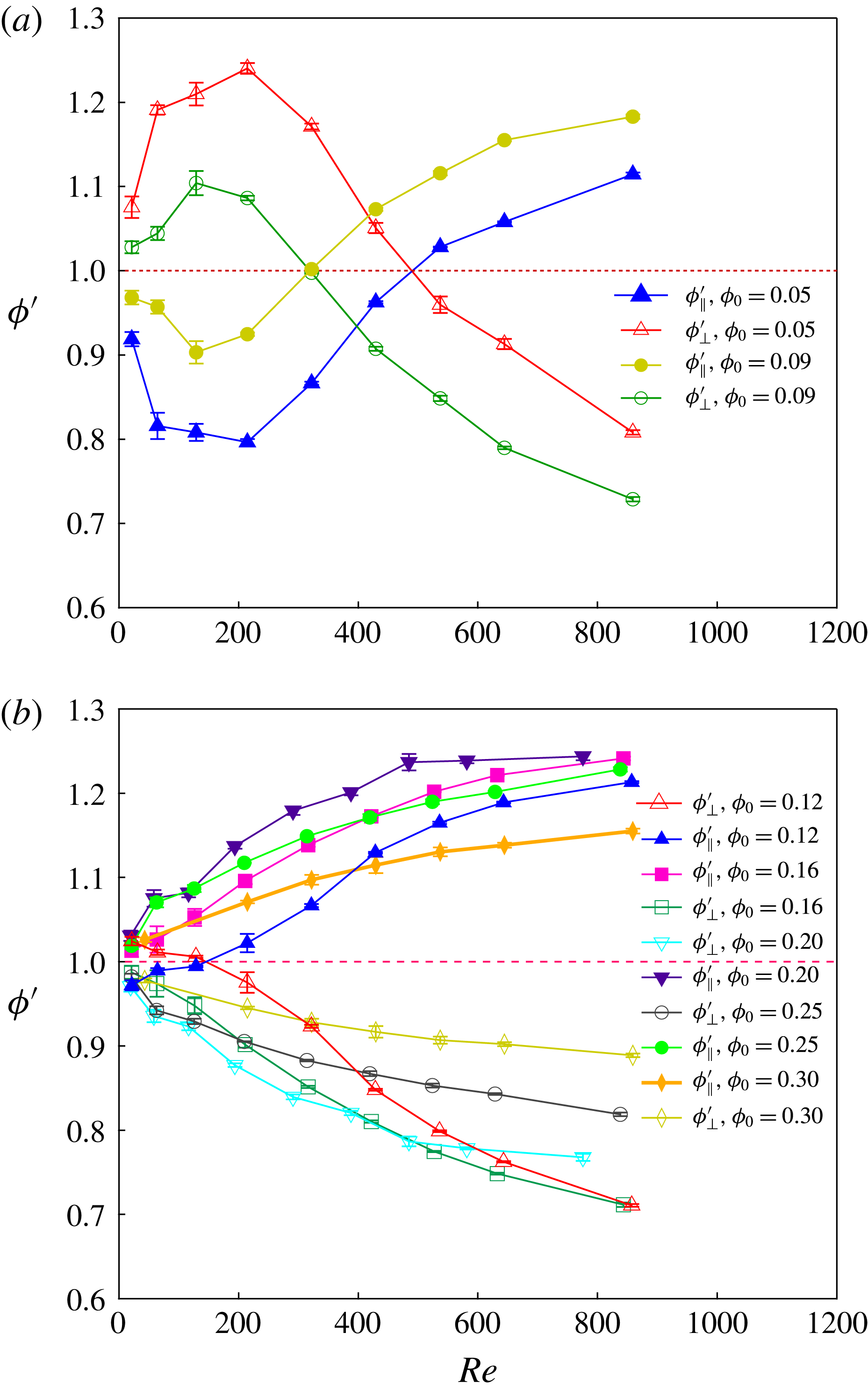
The concentrations in the two downstream branches are shown in figure 9, where we have plotted the normalized solid fractions given by
 $\unicode[STIX]{x1D719}_{\Vert }^{^{\prime }}=\unicode[STIX]{x1D719}_{\Vert }/\unicode[STIX]{x1D719}_{0}$
and
 $\unicode[STIX]{x1D719}_{\bot }^{^{\prime }}=\unicode[STIX]{x1D719}_{\bot }/\unicode[STIX]{x1D719}_{0}$
, as functions of
 $Re$
;
 $\unicode[STIX]{x1D719}_{\Vert }$
and
 $\unicode[STIX]{x1D719}_{\bot }$
are the measured mean solid volume fractions in the straight and side outlet branches, respectively. There is a distinct change seen between the dilute
 $\unicode[STIX]{x1D719}_{0}$
and
 $\unicode[STIX]{x1D719}_{0}\geqslant 0.12$
. For
 $0.05\leqslant \unicode[STIX]{x1D719}_{0}\leqslant 0.09$
, the previously noted
 $\unicode[STIX]{x1D6FD}_{\mathit{particle}}$
behaviour leads to a complex behaviour of the solid loading. With increasing
 $Re$
,
 $\unicode[STIX]{x1D719}_{\bot }^{^{\prime }}$
increases then decreases with an opposite trend for
 $\unicode[STIX]{x1D719}_{\Vert }^{^{\prime }}$
. For higher inlet solid fractions,
 $0.12\leqslant \unicode[STIX]{x1D719}_{0}\leqslant 0.30$
, the straight outlet branch grows progressively more concentrated, and the side branch more dilute, as
 $Re$
increases. The basis for this behaviour appears to be that at high
 $Re$
, particle migration towards the centre of the channel results in more particles entering the straight branch. When combined with the reduced fluid flux into the straight channel under these concentrated conditions, the mean concentration
 $\unicode[STIX]{x1D719}_{\Vert }$
in the straight channel is further increased. The result is an increased effective viscosity in the straight branch, which further reduces flow to the straight branch; recall that the mean pressure gradients in the outlet channels are equal and thus the flux is expected to be reduced in the channel with higher solids loading. The inlet branch flow thus affects the hydraulic relation of flux to pressure drop in the outlet branches.
Mean outlet branch particle volume fraction, normalized by inlet fraction, for particles of
 $d/D=0.1$
. (a)
 $0.05\leqslant \unicode[STIX]{x1D719}_{0}\leqslant 0.09$
and (b)
 $0.12\leqslant \unicode[STIX]{x1D719}_{0}\leqslant 0.30$
.

The effect of particle size was considered by studying suspensions of larger particles of average diameter
 $d=480$
 $\unicode[STIX]{x1D707}$
m, yielding
 $d/D=0.2$
. Experiments only for
 $\unicode[STIX]{x1D719}_{0}=0.05$
and
 $\unicode[STIX]{x1D719}_{0}=0.25$
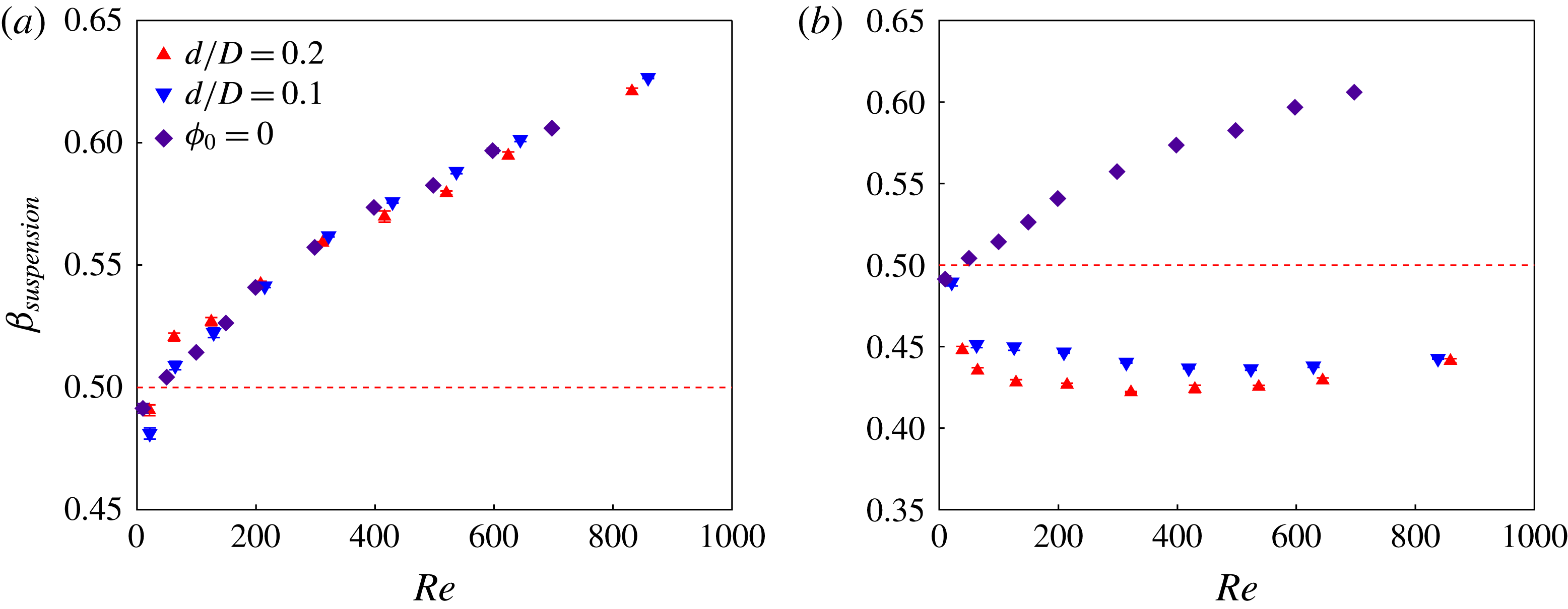
were performed for these larger particles. Figure 10 compares
 $\unicode[STIX]{x1D6FD}_{\mathit{suspension}}$
for the two
 $d/D$
. For
 $\unicode[STIX]{x1D719}_{0}=0.05$
, particle size has a negligible effect on
 $\unicode[STIX]{x1D6FD}_{\mathit{suspension}}$
, which for both sizes agrees with the pure fluid result. For
 $\unicode[STIX]{x1D719}_{0}=0.25$
,
 $\unicode[STIX]{x1D6FD}_{\mathit{suspension}}$
of both sizes deviates from that of the pure fluid, with
 $\unicode[STIX]{x1D6FD}_{\mathit{suspension}}<0.5$
; for
 $d/D=0.2$
there is a slightly stronger deviation from the pure fluid result, i.e. a slightly smaller
 $\unicode[STIX]{x1D6FD}_{\mathit{suspension}}$
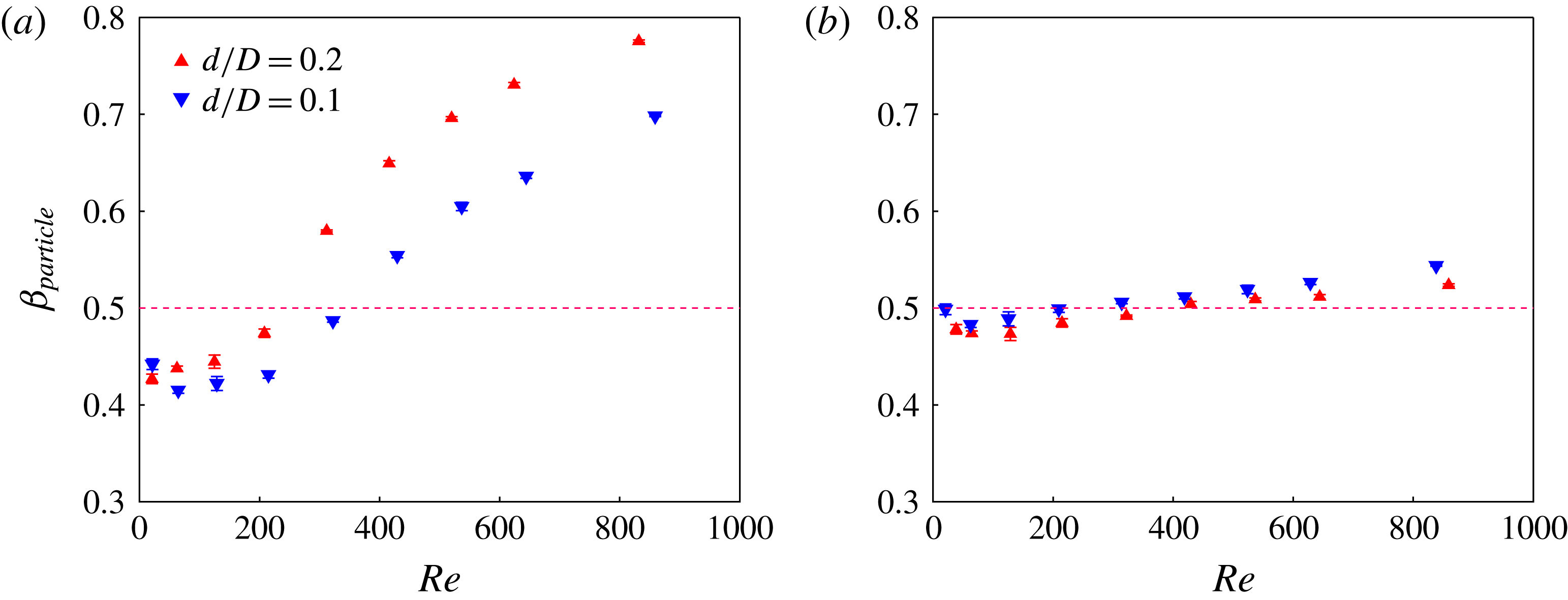
. Figure 11 shows the effect of particle size on
 $\unicode[STIX]{x1D6FD}_{\mathit{particle}}$
. For
 $\unicode[STIX]{x1D719}_{0}=0.25$
, little influence of particle size is observed. For
 $\unicode[STIX]{x1D719}_{0}=0.05$
, we find similar partitioning of the particles for both
 $d/D$
at lower
 $Re$
where
 $\unicode[STIX]{x1D6FD}_{\mathit{particle}}<0.5$
; at larger
 $Re$
, where the trend is reversed, and particles tend to preferentially follow the straight channel, larger particles reach
 $\unicode[STIX]{x1D6FD}>0.5$
at smaller
 $Re$
and have a significantly higher
 $\unicode[STIX]{x1D6FD}_{\mathit{particle}}$
.
Effect of particle size on bulk flow partitioning. Plots for
 $d/D=0.1$
and
 $0.2$
of
 $\unicode[STIX]{x1D6FD}_{\mathit{suspension}}$
at (a)
 $\unicode[STIX]{x1D719}_{0}=0.05$
and (b)
 $\unicode[STIX]{x1D719}_{0}=0.25$
.

Effect of particle size on particle partitioning. Plots for
 $d/D=0.1$
and
 $0.2$
of
 $\unicode[STIX]{x1D6FD}_{\mathit{particle}}$
at (a)
 $\unicode[STIX]{x1D719}_{0}=0.05$
and (b)
 $\unicode[STIX]{x1D719}_{0}=0.25$
.

4.2 Lattice-Boltzmann analysis of particle migration
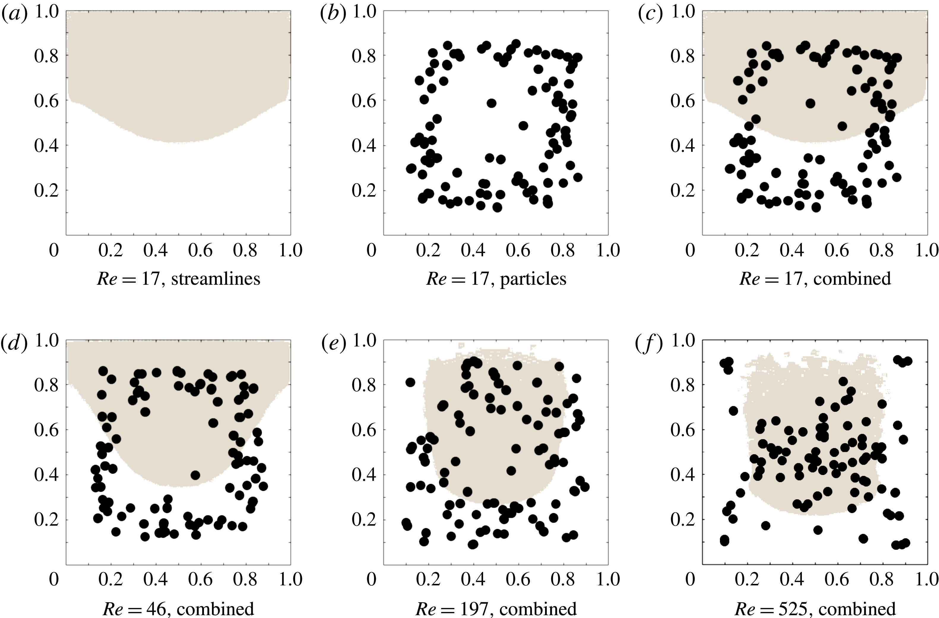
In this section, we first show the results of the combined lattice-Boltzmann discrete-particle simulation for a straight channel coupled with streamlines for the T-geometry. In figure 12, for several
 $Re$
the zones from which computed streamlines proceeding to each downstream branch are delineated by different shading; COMSOL- and CDP-calculated streamlines agree almost exactly for these zones. The zones are shown at a position well upstream of, and thus unaffected by, the bifurcation. Particle positions determined by a lattice-Boltzmann simulation in a periodic straight channel as described in § 3.2 are shown as well. In figure 12(a–c), the combined streamline and particle location analysis is illustrated for
 $Re=17$
by showing the streamlines and particle positions, then the combination of the two. In figure 12(d–f), the combined information is shown for
 $Re=46$
,
 $197$
and
 $525$
, respectively. The resulting particle split
 $\unicode[STIX]{x1D6FD}_{\mathit{particle}}$
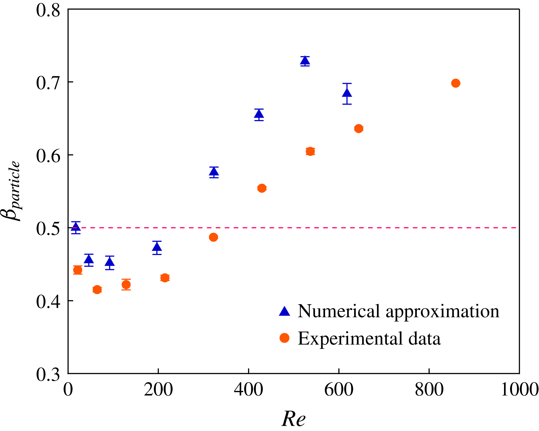
is determined from the procedure simply by computing the flux associated with streamlines occupied by particles (using the velocity information) and those which are unoccupied; the result is shown in figure 13. The prediction captures the basic trend of the experimental data, with
 $\unicode[STIX]{x1D6FD}_{\mathit{particle}}<0.5$
and decreasing for the lower range of
 $Re$
, reaching a minimum and then turning to
 $\unicode[STIX]{x1D6FD}_{\mathit{particle}}>0.5$
at higher
 $Re$
. The predicted
 $\unicode[STIX]{x1D6FD}_{\mathit{particle}}$
lies generally above the experimental data over the entire range of
 $Re$
. In the experiments, some level of migration may occur in the short circular inlet tube which carries the fluid from the barrel of the syringe to the entrance of the square channel. Despite the quantitative difference, the qualitative agreement clearly supports the hypothesis that the trend in the particle split at dilute conditions can be ascribed to inertial migration in the upstream branch.
Inlet migration analysis combined with fluid streamlines in the bifurcation. Shaded areas represent the streamline regions leading to the straight branch, unshaded go to the side branch. The procedure is illustrated for
 $Re=17$
: (a) computed streamline zones, (b) lattice-Boltzmann computed particle locations for
 $d/D=0.1$
after axial flow to a mean distance corresponding to the experimental entrance length (
 $L/D=58$
) and (c) the superimposed particle positions and streamline regions. Combined plots are shown for (d)
 $Re=46$
, (e)
 $Re=197$
and (f)
 $Re=525$
.

Numerical prediction of the combined analysis described by the prior figure for
 $\unicode[STIX]{x1D6FD}_{\text{particles}}$
at
 $\unicode[STIX]{x1D719}_{0}=0.05$
.

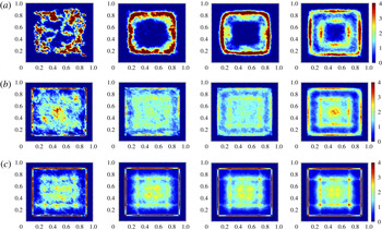
The migration in the straight channel has also been analysed by LB simulation for higher solid fractions, allowing the result to go to full development. In figure 14, the particle centre density distributions computed are shown for
 $d/D=0.2$
and
 $\unicode[STIX]{x1D719}=0.05$
, 0.15 and 0.25, for a subset of values of
 $Re$
displaying the basic features. It should be noted that the values of these densities are normalized by the mean and are upper limited to a value of 4, but for localized positions considerably higher values are found, particularly in the corners: the maximum values in figure 14(a) for
 $\unicode[STIX]{x1D719}_{0}=0.05$
at
 $Re=9.2$
, 46, 92 and 276 are 19.1, 14.3, 9.3 and 6.3; figure 14(b) for
 $\unicode[STIX]{x1D719}_{0}=0.15$
, the respective values are 36.8, 4.2, 3.4 and 4.7; figure 14(c) for
 $\unicode[STIX]{x1D719}_{0}=0.25$
, the respective values are 68.0, 67.0, 52.5 and 28.5. The particle centres accumulate in a distinct layer at the wall with some particles in the core at smaller
 $Re$
, followed by progressively stronger migration toward the core with increasing
 $Re$
. At
 $\unicode[STIX]{x1D719}_{0}=0.05$
and low
 $Re$
, only weak migration is seen as viscous hydrodynamic interactions may disrupt the organized structure; as
 $Re$
increases, there is a development of a distinct ‘ring’ at
 $Re=46$
and 92, which gives way to a combined ring and core region at
 $Re=276$
. Use of the pure fluid streamlines with these profiles fails to predict the observed partitioning, shown in figure 11 to be
 $\unicode[STIX]{x1D6FD}_{\mathit{particle}}\approx 0.5$
and only weakly dependent on
 $Re$
; the plots are not shown, but we find for both
 $\unicode[STIX]{x1D719}_{0}=0.15$
and 0.25 that
 $\unicode[STIX]{x1D6FD}_{\mathit{particle}}>0.5$
and increasing with
 $Re$
, with higher values for
 $\unicode[STIX]{x1D719}_{0}=0.25$
.
Particle centre distribution following migration to full development in straight channel flow computed by the lattice-Boltzmann method at (a)
 $\unicode[STIX]{x1D719}_{0}=0.05$
, (b)
 $\unicode[STIX]{x1D719}_{0}=0.15$
and (c)
 $\unicode[STIX]{x1D719}_{0}=0.25$
. From left to right at each
 $\unicode[STIX]{x1D719}_{0}$
, the Reynolds number based on pure fluid viscosity is
 $Re=9.2$
, 46, 92 and 276. The colour bar indicates the particle centre density normalized by its average value, and is upper limited at a value of 4 to allow visualization of lower values; higher values are found within zones corresponding to this upper limit (see text for more detail).

4.3 Immersed boundary simulations
In this section, we present fully resolved particle-laden flow in the T-channel at
 $\unicode[STIX]{x1D719}_{0}=0.05$
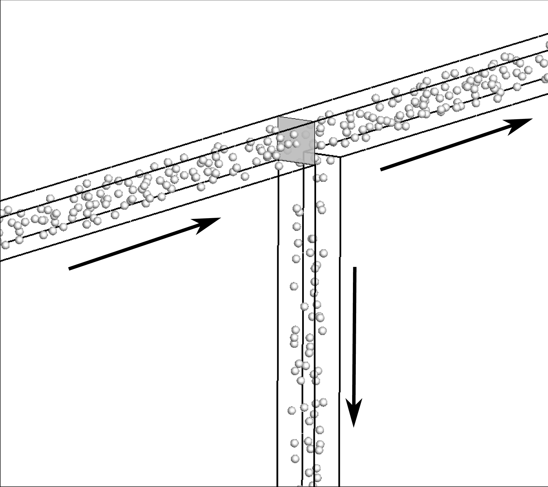
. Figure 15 shows a snapshot from an IB simulation for
 $Re=100$
and
 $d/D=0.2$
. Note that the observed particle split is
 $\unicode[STIX]{x1D6FD}_{\mathit{particle}}=0.53$
, but the particles in the straight channel seem more ‘crowded’ than in the side channel near the bifurcation. The flow is decelerating along the straight channel, but accelerating along the side channel in the vicinity of the bifurcation, and thus particles crowd in the straight channel, but not in the side channel. This may explain why
 $\unicode[STIX]{x1D6FD}_{\mathit{particle}}$
and
 $\unicode[STIX]{x1D6FD}_{\mathit{suspension}}$
decrease with increasing
 $\unicode[STIX]{x1D719}_{0}$
as the crowding creates a blockage in the straight channel, which, in turn, drives flow towards the side channel (figure 8
b).
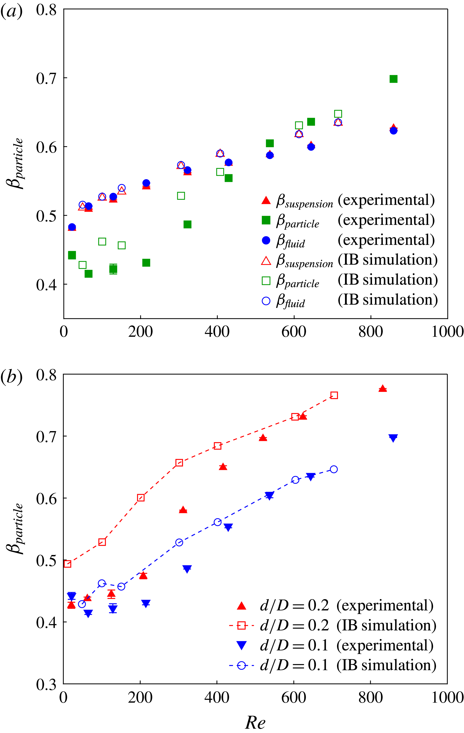
Figure 16(a) compares the flow ratios measured experimentally with the predictions from IB simulations for
 $d/D=0.1$
. The simulation results for
 $\unicode[STIX]{x1D6FD}_{\mathit{suspension}},\unicode[STIX]{x1D6FD}_{\mathit{particle}}$
and
 $\unicode[STIX]{x1D6FD}_{\mathit{fluid}}$
are in fairly good agreement with the experiments. The simulations capture the trend of
 $\unicode[STIX]{x1D6FD}_{\mathit{particle}}<0.5$
for the lower range of
 $Re$
as well as the increase for larger
 $Re$
. Figure 16(b) compares the effect of particle size. Consistent with the experimental trend,
 $\unicode[STIX]{x1D6FD}_{\mathit{particle}}$
is larger for the larger particle size. The IB simulations predict larger
 $\unicode[STIX]{x1D6FD}_{\mathit{particle}}$
than seen experimentally, particularly at lower
 $Re$
for
 $d/D=0.2$
. In contrast to the experiments, we do not observe
 $\unicode[STIX]{x1D6FD}_{\mathit{particle}}<0.5$
at lower
 $Re$
for
 $d/D=0.2$
.
Snapshot of an immersed boundary simulation for
 $d/D=0.2,\unicode[STIX]{x1D719}_{0}=0.05$
and
 $Re=100$
showing greater particle density in the straight channel beyond the bifurcation. Analysis of particle splits projected back to the shaded plane just before the bifurcation is presented in figures 19 and 20.

Comparison of immersed boundary simulation results and experiment at
 $\unicode[STIX]{x1D719}_{0}=0.05$
. (a) Fluid, particle and suspension flow ratios for
 $d/D=0.1$
and (b) effect of particle size on particle flow ratio.

In order to understand the behaviour of particles in the vicinity of the bifurcation, we computed the normalized average distribution of particle positions at the junction. This distribution was computed by considering the whole set of particle positions across the entire simulation and binning the observations based on the particle centre
 $x$
and
 $y$
locations, resulting in a time and depth (
 $z$
-coordinate) averaged estimate, and then normalizing it to the range
 $[0,1]$
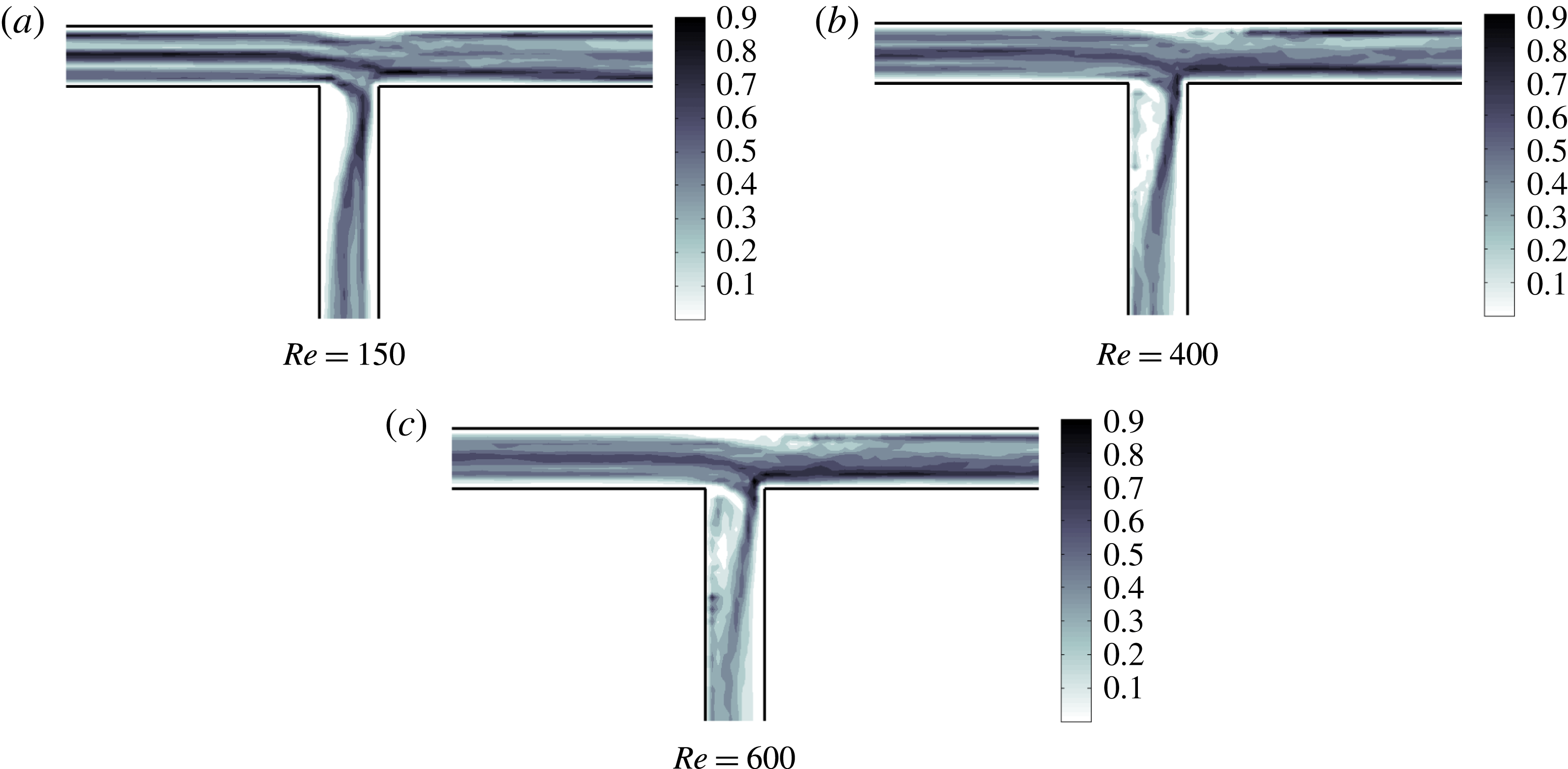
. Figure 17 shows the distribution for different Reynolds numbers for
 $d/D=0.2$
. The distribution for
 $Re=150$
(figure 17
a) shows the depletion of particles in the two recirculation zones, one on the straight channel branch and the other in the side channel branch, with the latter being more significant. At this
 $Re$
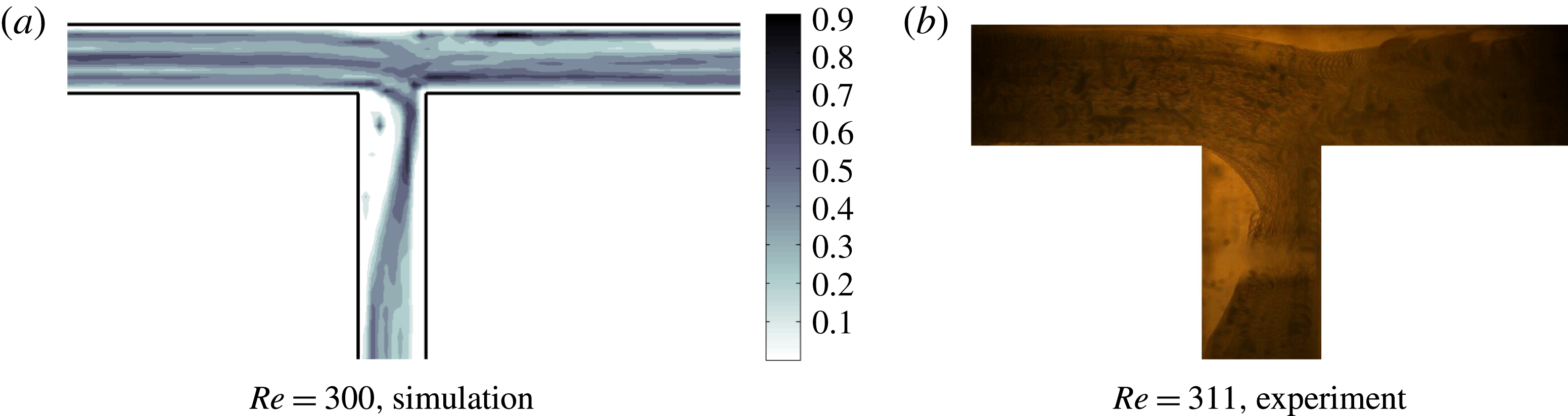
, none of the particles break into the recirculation zone in the side branch. A visual comparison of the time-averaged view from experiment at
 $Re=311$
(which shows the entire particle volume) and simulation at
 $Re=300$
(particle centres) is given by figure 18; here, a few particles enter the recirculation zones and are trapped for a period of time. The average number of particles which remain transiently trapped in the side recirculation zone increases with
 $Re$
as shown in figure 17(b) and figure 17(c) for
 $Re=400$
and 600, respectively, resulting in a higher blockage to the side channel; this increase in transient trapping of particles with
 $Re$
is seen also in the experimental videos described above.
Particle distribution from immersed boundary simulation in the vicinity of the bifurcation averaged over time and depth for
 $d/D=0.2$
.

Particle distribution in the vicinity of the bifurcation averaged over time for
 $d/D=0.2$
. (a) Immersed boundary simulation at
 $Re=300$
and (b) experiment at
 $Re=311$
. Experimental data in (b) are a direct overlap of images of entire particles, while the simulation data are centre positions only, averaged also over depth.

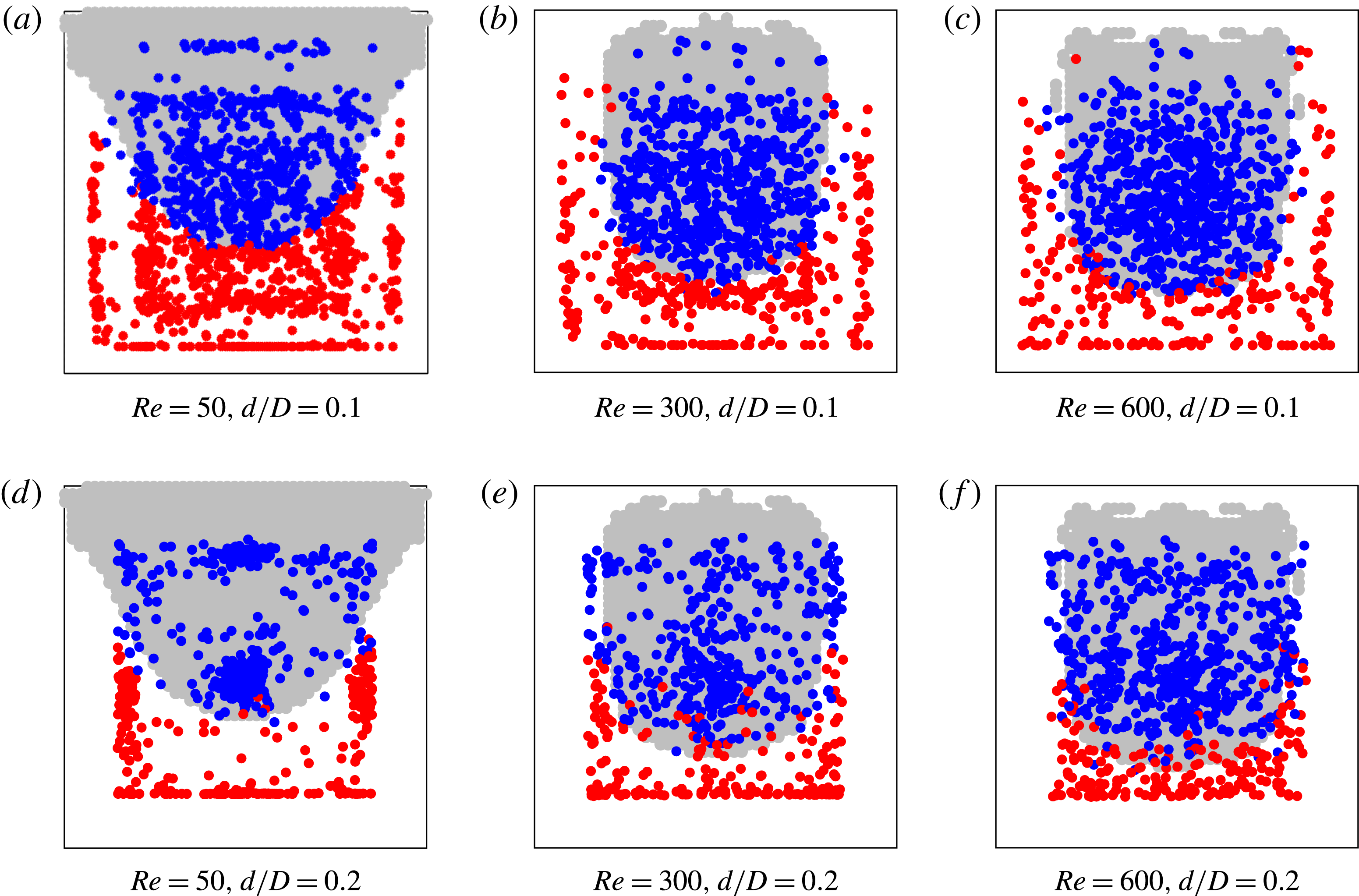
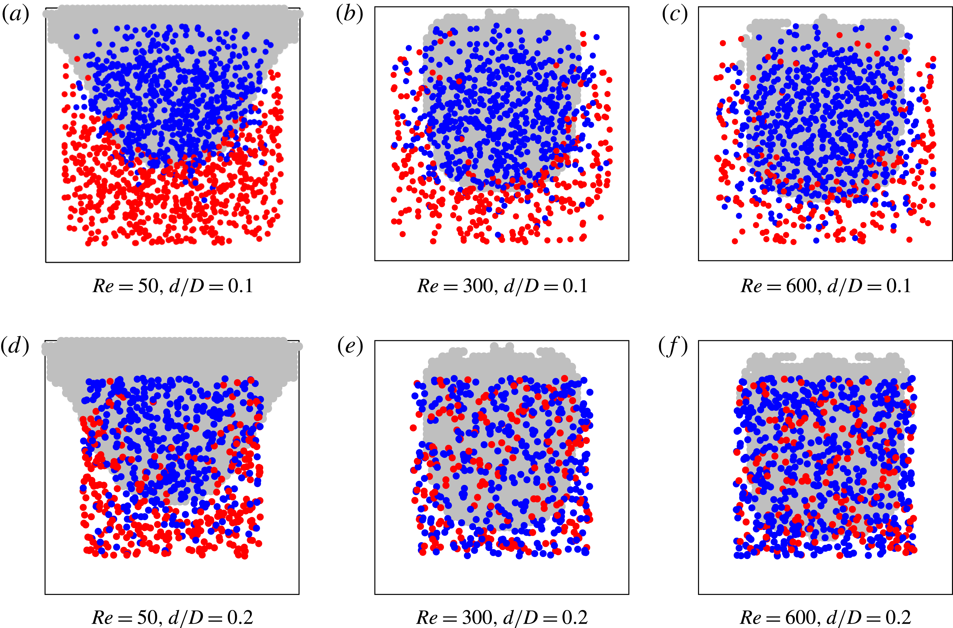
We analyse the particle split in a cross-section just before the bifurcation in figure 19 for
 $d/D=0.1$
and 0.2. We plot all the particles which passed through the shaded plane in figure 15 over the duration of the simulation and colour code them based on whether they flowed to the straight or side channel. For the smaller particles with
 $d/D=0.1$
, the particle split boundary coincides very well with the streamline split boundary. However for
 $d/D=0.2$
, more particles inside the capture region turn at the junction, particularly at higher
 $Re$
. Also with increasing
 $Re$
, the dividing curve (which separates the two sets of particles) moves toward the side channel. Interestingly, at
 $Re=50$
and
 $d/D=0.2$
, the particle distribution at the junction is concentrated at the centre of the cross-section and the periphery of the cross-section, with a banded region between where particles are less likely to be found. There is some asymmetry in the distribution of the particles in the cross-section, indicating that the bifurcation has some influence on this cross-section, and the decoupling of the streamlines from the particle migration shown above can thus only be qualitative in its predictions. Migration is seen to generate a near-wall layer and particles on the interior for
 $d/D=0.1$
and
 $Re=50$
, with more migration toward the centre at
 $Re=300$
and 600. For the particles of
 $d/D=0.2$
, migration into a wall layer and a more isolated core region is found at
 $Re=50$
, with a more dispersed core region found at
 $Re=300$
and a core region visible at
 $Re=600$
but with a relatively uniform lower density of particle centres surrounding it; the migration to the centre is seen in the lattice-Boltzmann calculations shown in figure 14, but only at
 $Re=276$
, suggesting the simulations here may be capturing a transient behaviour. The formation of the wall layer at the smaller
 $Re$
and transition toward migration to the central zone is directionally consistent with findings of Miura et al. (Reference Miura, Itano and Sugihara-Seki2014), but the axial distance needed for full development is found by these authors to be much larger than the
 $L_{0}/D=58$
in this work. The concentration here is
 $\unicode[STIX]{x1D719}_{0}=0.05$
, much larger than the solid fractions of
 $1.6{-}2.4\times 10^{-4}$
in Miura et al.’s study, so particle interactions play a significant role here.
While the noted interactions between particles have not been examined in detail, their influence is made clearer by using a feature of simulations, namely that each particle can be tracked from its outlet channel back to its inlet position, i.e. where all particles are released. The distributions corresponding to the two particle sizes are strikingly different at the inlet cross-section, illustrated in figure 20. The particle split is quite different from the fluid streamline split for both cases, showing that there is significant cross-streamline motion of the particles. The particles are well mixed at the inlet for high Reynolds numbers for
 $d/D=0.2$
, showing that there is significant particle interaction as well as migration at play in the flow. Comparison with the behaviour at very dilute conditions misses important phenomena; this was shown by Han et al. (Reference Han, Kim, Kim and Lee1999) as there was significant dispersion around the expected inertial migration equilibrium position from the theory (Asmolov Reference Asmolov1999; Matas et al.
Reference Matas, Morris and Guazzelli2009) at
 $\unicode[STIX]{x1D719}=0.06$
and evidence of both inertial and shear-induced migration (Hampton et al.
Reference Hampton, Mammoli, Graham, Tetlow and Altobelli1997) at small
 $Re$
and
 $\unicode[STIX]{x1D719}=0.1$
.
Analysis of particle flow ratio at a cross-section just before the bifurcation at
 $\unicode[STIX]{x1D719}_{0}=0.05$
from immersed boundary method simulations. The symbols ● (red) and ● (blue) denote particles which turn into the side channel and continue to the straight channel, respectively.

Analysis of particle flow split at a cross-section near the inlet for
 $\unicode[STIX]{x1D719}_{0}=0.05$
from immersed boundary method simulations. The symbols ● (red) and ● (blue) denote particles which turn into the side channel and continue to the straight channel, respectively.

5 Concluding remarks
We have studied the flow of suspensions through a square cross-section channel with an asymmetric T-bifurcation. To simplify the problem, we have considered a basic bifurcation, with both downstream channels having the same length, pressure drop and cross-sectional area. The primary goal of the work was to understand whether and how solid loading, under neutrally buoyant conditions, leads to a difference from single-phase Newtonian fluid flow and how such a deviation depends on Reynolds number. Focusing the characterization on the bulk partitioning to the two downstream branches, we measure the ratio of the fluxes to each downstream branch:
 $\unicode[STIX]{x1D6FD}=Q_{\Vert }/Q_{0}$
, with a specification to the appropriate material. Based on examination of this measure, we have found fundamental differences in pure fluid and suspension partitioning at a flow bifurcation.
For a Newtonian fluid, figure 5 shows that the flow partitions equally at small
 $Re$
and progressively more to the straight channel as flow rate increases, i.e.
 $\unicode[STIX]{x1D6FD}>0.5$
and increases with
 $Re$
. To summarize how the suspension components partition in the experiments conducted, consider figures 6–9. Figure 6 shows that under dilute conditions, at inlet solid fraction
 $\unicode[STIX]{x1D719}_{0}=0.05$
, the suspension partitions essentially as the pure fluid, with
 $\unicode[STIX]{x1D6FD}_{\mathit{suspension}}>0.5$
and increasing with
 $Re$
. However, at this condition, the particle split exhibits non-monotonic dependence on
 $Re$
, first decreasing to
 $\unicode[STIX]{x1D6FD}_{\mathit{particle}}<0.5$
and then increasing to surpass 0.5 as
 $Re$
increases. This is rationalized by a consideration of the upstream migration combined with the pure fluid streamlines in the bifurcation, which leads to particles near the walls at small
 $Re$
, with development of a higher concentration of particles toward the core at larger
 $Re$
. The influence of the particles on the downstream wall shear stress is too small for the added particles to affect the bulk behaviour, and hence
 $\unicode[STIX]{x1D6FD}_{\mathit{suspension}}(Re)\doteq \unicode[STIX]{x1D6FD}(Re)$
for the pure fluid over all
 $Re$
studied. At higher
 $\unicode[STIX]{x1D719}$
, figure 7 shows that the curve of
 $\unicode[STIX]{x1D6FD}_{\mathit{suspension}}(Re)$
becomes progressively more weakly increasing with
 $Re$
until
 $\unicode[STIX]{x1D719}=0.16$
and is decreasing with
 $Re$
with all values below
 $\unicode[STIX]{x1D6FD}_{\mathit{particle}}=0.5$
for
 $\unicode[STIX]{x1D719}\geqslant 0.2$
. This finding, that the majority of the suspension exits through the side channel at large
 $Re$
, is in striking contrast in behaviour relative to pure fluid. This result becomes clearer when we consider that
 $\unicode[STIX]{x1D6FD}_{\mathit{particle}}>\unicode[STIX]{x1D6FD}_{\mathit{fluid}}$
for the elevated
 $\unicode[STIX]{x1D719}$
in figure 8, and this is reflected in an increase of the solid volume fraction in the straight outlet branch, as shown in figure 9.
It is evident that multiphase flow concepts are critical to understanding the dynamics observed for the suspension, i.e. one must account for each of the components of the mixture. In particular, explanation of the observed behaviour requires consideration of how upstream particle migration impacts on both the fluid mechanics in the bifurcation and the flow resistance in the two downstream channels, and we have utilized simulation tools to extract information on the migration aspect. Complete discrete-particle simulation of the problem is now becoming accessible, but for the advanced immersed boundary tool used here, such simulation was only feasible for smaller solid fractions. The established lattice-Boltzmann method for suspensions provided insight into the migration and its influence on the partitioning of the particles. Under dilute particle conditions, the bulk mixture flow is close to that of the single-phase flow but the particle flux ratio in the downstream branches following the bifurcation does not follow expectations based on a uniform distribution. At large
 $\unicode[STIX]{x1D719}_{0}$
, the bulk flow itself would be poorly predicted by an effective medium description of the mixture based on effective rheological properties depending upon solid fraction, as is evident from the
 $\unicode[STIX]{x1D719}$
-dependence of the data deviating strongly from the effective medium prediction (with uniform properties) given by figure 7(b); as seen in our lattice-Boltzmann simulations presented here, there is significant migration, which at the higher values of
 $\unicode[STIX]{x1D719}$
is expected to involve shear-induced migration (Hampton et al.
Reference Hampton, Mammoli, Graham, Tetlow and Altobelli1997; Ahmed & Singh Reference Ahmed and Singh2011) coupled with inertial migration as seen in earlier work in tube flow by Han et al. (Reference Han, Kim, Kim and Lee1999). This migration results in an abundance of particles going to the straight outlet and the increased values of
 $\unicode[STIX]{x1D719}_{\Vert }$
, seen in figure 9, increase the effective viscosity of the material. Thus the flow resistance in the straight channel is larger and there is a consequent reduction in the flow which can be achieved at the available pressure drop. This influence of the particle distribution in the upstream and bifurcation on the hydraulic relation of flux to pressure gradient in the downstream branch has not been recognized in prior work. Shear-induced migration acting alone, i.e. at small
 $Re$
, does not result in substantial deviation of the split from the pure fluid Stokes flow
 $\unicode[STIX]{x1D6FD}\doteq 0.5$
. This is apparently a result of the symmetry of the migration in the square conduit (see figure 14 for examples of this) and near symmetry of the streamline split as
 $Re\rightarrow 0$
. To see the latter point, consider the more balanced streamline zones in figure 12(a) at
 $Re=17$
, relative to the higher
 $Re$
streamline zones in the same figure.
The detailed behaviour in the vicinity of the bifurcation deserves further study. A separation zone in which the concentration is difficult to predict and generally well below the bulk appears at the corner entering the side channel at
 $Re\geqslant 50$
. Another closed streamline zone appears at the channel wall opposite the side channel. The flow has a complex three-dimensional structure in this vicinity, with fluid to the side branch drawn from the entire near-wall region at elevated
 $Re$
. Such flow structures combined with the multiphase effects require detailed resolution to allow modelling and prediction of flow processes involving bifurcating channels. At the higher volume fractions studied here, the influence of bulk rheology due to the particles, as well as their collisions with the corner region, are expected to be influential on the mean streamline pattern. The ability of continuum modelling in which particles are a distributed phase, such as two-fluid modelling, to capture such behaviour for the high-
 $Re$
conditions studied here is presently very limited. Advances in this area of study would have major engineering value.
Acknowledgements
The work at CUNY City College of New York was supported in part by Halliburton. The work at Stanford University was supported by the US Army High Performance Computing Research Center (AHPCRC) and also by Stanford University’s Certainty computer cluster, which is funded by the American Recovery and Reinvestment Act (ARRA) of 2009 (grant no. W911NF07200271). Computational study at CUNY City College was supported by a grant of computer time from the City University of New York High Performance Computing Center under NSF Grants CNS-0855217, CNS-0958379 and ACI-1126113.
Supplementary movies
Supplementary movies are available at https://doi.org/10.1017/jfm.2018.183.