


1. Introduction
Since the experimental work of Reynolds (Reference Reynolds1883), who firstly observed subcritical transition to turbulence in a wall-bounded shear flow, the dynamics of transition has remained an open problem of fluid dynamics. One of the most intriguing features of transitional flows is that turbulence does not arise at the same time in the whole domain, being preceded by the formation of localized flow structures that grow in amplitude and spread in space. The first of these localized flow features to be observed were turbulent spots, which have been investigated by many researchers in the past. Emmons (Reference Emmons1951) was the first to show experimentally, for a boundary-layer flow over a flat plate, that turbulent spots may trigger turbulence; later, this was confirmed experimentally and numerically in plane channel flow, analysing the spot characteristics (Carlson, Widnall & Peeters Reference Carlson, Widnall and Peeters1982; Henningson & Kim Reference Henningson and Kim1991; Klingmann Reference Klingmann1992; Aida, Tsukahara & Kawaguchi Reference Aida, Tsukahara and Kawaguchi2010, Reference Aida, Tsukahara and Kawaguchi2011; Lemoult, Aider & Wesfreid Reference Lemoult, Aider and Wesfreid2013; Lemoult et al. Reference Lemoult, Gumowski, Aider and Wesfreid2014). In pipe flows, other localized flow structures – dubbed puffs – are observed both numerically and experimentally (Eckhardt et al. Reference Eckhardt, Schneider, Hof and Westerweel2007; Avila et al. Reference Avila, Moxey, de Lozar, Avila, Barkley and Hof2011). Puffs are localized, downstream-travelling flow structures within a laminar field, sustained by the energy provided by the neighbouring laminar motion at the upstream end of the puff. They can decay, split or merge, filling the laminar flow with turbulent fluctuations. More recently, Duguet, Schlatter & Henningson (Reference Duguet, Schlatter and Henningson2010) have shown that when locally perturbing the plane Couette flow, the fully turbulent state is preceded by the formation of turbulent bands. The same behaviour was reported by Tao & Xiong (Reference Tao and Xiong2013) and Xiong et al. (Reference Xiong, Tao, Chen and Brandt2015), who have shown that after injecting a localized perturbation, turbulent bands grow obliquely in the domain until decay or breakdown to turbulence. In the latter case, it was assessed that the turbulent bands’ lifetime is longer than that of turbulent spots. Besides having a crucial role in turbulent transition, oblique turbulent bands characterize also the (transient) turbulent state in shear flows at low Reynolds numbers, as shown by Tsukahara et al. (Reference Tsukahara, Seki, Kawamura and Tochio2005). In fact, in the pipe, plane Couette and plane Poiseuille flow, there is a range of moderate Reynolds numbers for which experiments and numerical simulations have shown that turbulence is not fully extended in space, since localized regions characterized by laminar and turbulent behaviour coexist when the statistically steady turbulent state is reached. Indeed, elongated oblique self-sustained turbulent bands within a laminar flow appear in plane Couette flow at  $Re>290$ (Prigent et al. Reference Prigent, Grégoire, Chaté, Dauchot and van Saarloos2002; Barkley & Tuckerman Reference Barkley and Tuckerman2005; Duguet et al. Reference Duguet, Schlatter and Henningson2010; Tuckerman & Barkley Reference Tuckerman and Barkley2011), and in plane Poiseuille flow for
 $Re\geqslant 1000$ (Tsukahara, Kawaguchi & Kawamura Reference Tsukahara, Kawaguchi and Kawamura2014; Tuckerman et al. Reference Tuckerman, Kreilos, Schrobsdorff, Schneider and Gibson2014; Tao, Eckhardt & Xiong Reference Tao, Eckhardt and Xiong2018; Shimizu & Manneville Reference Shimizu and Manneville2019; Kashyap, Duguet & Dauchot Reference Kashyap, Duguet and Dauchot2020). In the channel flow, turbulent–laminar oblique patterns were observed experimentally for
 $Re = 1000$ by Carlson et al. (Reference Carlson, Widnall and Peeters1982). Numerical simulations reproduced these patterns also at lower Reynolds numbers (Xiong et al. Reference Xiong, Tao, Chen and Brandt2015; Tao & Xiong Reference Tao and Xiong2017; Kashyap et al. Reference Kashyap, Duguet and Dauchot2020), estimating a threshold value for observing turbulent bands at
 $Re \approx 660$, according to Tao et al. (Reference Tao, Eckhardt and Xiong2018). Recently, Gomé, Tuckerman & Barkley (Reference Gomé, Tuckerman and Barkley2020) investigated the decay and splitting of these turbulent bands, finding that as the Reynolds number increases, their mean decay time increases and the mean splitting time decreases. At the ‘critical’ Reynolds number, estimated to be
 ${\approx }965$, these times are approximately equal. Thus it has been established that inclined bands persist for times of order
 $t \approx {O}(10^{5}\text {--}10^{6})$ only when
 $Re>965$, whereas they decay rapidly for lower values of
 $Re$. Song & Xiao (Reference Song and Xiao2020) reported recently the onset of such turbulent bands even at Reynolds number as low as
 $Re = 500$, generated by forcing the flow with a local perturbation with a sufficiently strong spanwise inflection. They showed that this forcing method permits us to generate bands at very low values of the Reynolds number, for which bands appeared previously to be not sustained. This procedure was motivated by the work of Xiao & Song (Reference Xiao and Song2020), where the authors performed a linear stability analysis of the mean velocity profile extracted in a small domain at the head of the turbulent band. By means of the stability analysis, it was suggested that spanwise inflectional instability may be the mechanism involved in the growth and self-sustaining process of turbulent bands.
In addition to the Reynolds number, the domain size plays an important role in the growth and self-interaction of turbulent bands. When the considered domain is sufficiently large, turbulent bands can grow for longer times, avoiding the probability of interaction with themselves or other bands. For this reason, several works studied the influence of the domain extension on the onset of turbulent bands. In order to reduce the computational cost, some numerical studies cleverly considered computational domains tilted in the direction of the bands, as done for plane Couette flow by Barkley & Tuckerman (Reference Barkley and Tuckerman2005) and for plane Poiseuille flow by Tuckerman et al. (Reference Tuckerman, Kreilos, Schrobsdorff, Schneider and Gibson2014). Very recently, Parente et al. (Reference Parente, Robinet, De Palma and Cherubini2021) carried out an optimal growth analysis in a tilted domain with given angle. They showed that although linear optimization is able to recover the main wavenumbers observed by direct numerical simulation, nonlinear effects are necessary for providing large-scale flow and spatial localization of the perturbation able to generate a turbulent band. Although very interesting for studying the dynamics of a single band, using the tilted domain constrains the turbulent bands to develop at a fixed angle and avoids (or reduces) the interactions with other bands, consequently resulting in a less rich dynamics. A more detailed analysis of laminar–turbulent patterns in shear flows is tackled in the review of Tuckerman, Chantry & Barkley (Reference Tuckerman, Chantry and Barkley2020).
In the literature, typically two strategies are used to obtain turbulent bands. The first consists in starting from a space-filling statistically steady turbulent state, and slowly decreasing the Reynolds number until patterned laminar regions in the initially turbulent flow begin to appear (Tsukahara et al. Reference Tsukahara, Seki, Kawamura and Tochio2005; Kashyap et al. Reference Kashyap, Duguet and Dauchot2020). This method usually leads to the formation of statistically steady laminar–turbulent patterns. Another method consists of perturbing the laminar flow with suitable localized disturbances having enough energy to trigger localized regions of turbulence eventually evolving into oblique stripes (Duguet et al. Reference Duguet, Schlatter and Henningson2010; Aida et al. Reference Aida, Tsukahara and Kawaguchi2010, Reference Aida, Tsukahara and Kawaguchi2011; Tao & Xiong Reference Tao and Xiong2013; Xiong et al. Reference Xiong, Tao, Chen and Brandt2015). When focusing on the second method, the amplitude, shape and localization of these initial perturbations should be chosen carefully to ensure their growth towards oblique bands. Depending on their shape, perturbations with higher amplitude may decay, while weaker perturbations may lead the flow to transition.
From a phase-space point of view, the problem of finding perturbations eventually generating these laminar–turbulent patterns consists of placing the starting point of the trajectory beyond the boundary of the basin of attraction of the laminar solution. Notably, the most relevant point of this boundary is its energy minimum, since it represents the minimal (in energy norm) perturbation of the laminar state that can lead the flow to transition. This point in the phase space has been dubbed, by Rabin, Caulfield & Kerswell (Reference Rabin, Caulfield and Kerswell2012), ‘minimal seed’ for turbulent transition. This energy minimum has been assessed for several shear flows, aiming at finding minimal energy thresholds for transition. In particular, in plane Couette flows, a minimal energy threshold varying with the Reynolds number as  $Re^{-2.7}$ has been found, in quantitative agreement with experimental estimates for pipe flows, whereas for the asymptotic-suction boundary layer, Cherubini, De Palma & Robinet (Reference Cherubini, De Palma and Robinet2015) found a scaling law of this energy threshold of
 $Re^{-2}$. Recently, Vavaliaris, Beneitez & Henningson (Reference Vavaliaris, Beneitez and Henningson2020) performed similar computations for a non-parallel boundary-layer flow but did not provide a scaling law with respect to the Reynolds number. The determination of these energy thresholds is of primary importance for control purposes, since passive or active control methods such as boundary manipulation (Rabin, Caulfield & Kerswell Reference Rabin, Caulfield and Kerswell2014) or profile flattening (Marensi, Willis & Kerswell Reference Marensi, Willis and Kerswell2019) able to increase this minimal energy would render these flows less prone to transition. However, to the authors’ knowledge, the minimal seed computation has never been carried out for the channel flow. In Farano et al. (Reference Farano, Cherubini, Robinet and De Palma2015, Reference Farano, Cherubini, Robinet and De Palma2016), a nonlinear optimization in channel flow has been performed for rather small target times, but without any energy bisection, which is needed for the determination of minimal seeds. Moreover, all the minimal seed computations reported in the literature, except those performed by Pringle, Willis & Kerswell (Reference Pringle, Willis and Kerswell2015) in a pipe flow, have been carried out in relatively small domains, hampering the development of laminar–turbulent patterns. In very large domains, where laminar–turbulent oblique bands exist, the minimal transition thresholds potentially can be different from those obtained in small domains. In fact, in small domains, the periodicity imposed in the streamwise and spanwise directions causes the interaction of the front of the perturbation with its tail already in the first phases of transition. Consequently, the kinetic energy of disturbances grows rapidly and suddenly saturates when turbulence fills the whole domain, whereas in large domains, the perturbations evolve freely for long times without interacting with themselves, so the development of disturbance appears to depart from that observed in smaller domains already at small times. As observed by several authors, the kinetic energy keeps growing for very long times, before saturating to a statistically steady value. Notably, in sufficiently large domains, localized perturbations often develop in an inclined direction with respect to the mean flow. Such a behaviour can be observed already at times comparable with the typical target times of minimal seed optimizations (i.e.
 ${O}(100)$). This difference in the dynamics of the perturbations depending on the domain size suggests that important differences can be found between minimal seeds computed in small and large domains, influencing the initial phases of formation of the band. Thus the analysis of these minimal perturbations and of their evolution towards oblique bands can potentially unveil the main mechanisms leading to the formation and sustainment of these laminar–turbulent patterns.
This work aims to find minimal seeds for the generation of turbulent bands in channel flow. The methodology to find these perturbations is based on the nonlinear variational optimization first used in the boundary-layer flow by Cherubini et al. (Reference Cherubini, De Palma, Robinet and Bottaro2010a, Reference Cherubini, De Palma, Robinet and Bottaro2011) and in pipe flow by Pringle & Kerswell (Reference Pringle and Kerswell2010) and Pringle, Willis & Kerswell (Reference Pringle, Willis and Kerswell2012), and then coupled with energy bisection by Rabin et al. (Reference Rabin, Caulfield and Kerswell2012) for the plane Couette flow and by other authors for other shear flows (Duguet et al. Reference Duguet, Monokrousos, Brandt and Henningson2013; Cherubini et al. Reference Cherubini, De Palma and Robinet2015; Vavaliaris et al. Reference Vavaliaris, Beneitez and Henningson2020). In all these studies, the kinetic energy was considered as the objective function of the optimization, and the optimal perturbations associated to the minimal input energy were localized spatially. Similar behaviour was found in Couette flow by Monokrousos et al. (Reference Monokrousos, Bottaro, Brandt, Di Vita and Henningson2011), maximizing the time integral of the entropy production. A detailed review of these methods is reported by Kerswell, Pringle & Willis (Reference Kerswell, Pringle and Willis2014) and by Kerswell (Reference Kerswell2018). In the present work, we carry out for the first time the computation of minimal seeds in channel flow for very large domains, allowing the creation of laminar–turbulent patterned final states such as oblique stripes. The perturbation kinetic energy is used as the objective function of the nonlinear optimization, which appears to be an appropriate choice since many literature studies report peaks of kinetic energy during the development of turbulent bands (Tao et al. Reference Tao, Eckhardt and Xiong2018). The minimal seeds obtained using this optimize-and-bisect method are found to change with the Reynolds number, presenting a power-law scaling of the initial energy  $E_{0_{min}} \propto Re^{-\gamma }$, with
 $\gamma$ being approximately four times larger than the values reported in other shear flows in smaller domains. Moreover, two distinct mechanisms of creation of turbulent bands are observed and discussed in detail.
The paper is organized in the following way. In § 2, the methodology is presented. In § 3, the main results of the optimization are reported and the nonlinear evolution in time of the optimal perturbation is discussed. Finally, in § 4, conclusions are drawn.
2. Problem formulation
The considered flow is a plane channel flow at Reynolds number  $Re = U_{c} H / \nu$, where
 $U_c$ is the centreline velocity of the laminar Poiseuille flow,
 $H$ is the half-width of the channel, and
 $\nu$ is the kinematic viscosity. The Reynolds number is varied by changing the pressure gradient, while the volume flux remains constant, with bulk velocity
 $U_b = 2/3$. The dynamics of this flow is studied by decomposing the instantaneous velocity field,
 ${\boldsymbol {u}}= [u,v,w]^{\rm T}$, into the laminar base flow
 $\boldsymbol {U} = [U(y), 0, 0]^{\rm T}$ and a perturbation
 $\boldsymbol {u}' = [u',v',w']^{\rm T}$. The dynamics of the perturbations of the laminar base flow is computed by solving the perturbative nonlinear incompressible Navier–Stokes equations:
 \begin{equation} \left.\begin{array}{ll} \displaystyle \frac{\partial u_i'}{\partial x_i} = 0,\\ \displaystyle \frac{\partial u_i'}{\partial t} + u_j'\,\frac{\partial u_i'}{\partial x_j} + u_j'\,\frac{\partial U_i}{\partial x_j} + U_j\,\frac{\partial u_i'}{\partial x_j} ={-} \frac{\partial p'}{\partial x_i} + \frac{1}{Re}\,\frac{\partial^{2} u_i'}{\partial {x_j^{2}}}, \end{array}\right\} \end{equation}
where  $\boldsymbol {U}=[U(y),0,0]^{\rm T}$,
 $U(y) = 1 - y^{2}$, is the laminar streamwise velocity profile,
 $p'$ is the pressure perturbation, and
 $x_i$ is the Cartesian reference frame having components
 $x, y, z$, for the streamwise, wall-normal and spanwise directions, respectively. No-slip boundary conditions are imposed at the walls for the three velocity components, while periodicity is fixed in the streamwise and spanwise directions.
In order to find the minimal seed for the considered flow, we first search for the optimal perturbation  $\boldsymbol {u}'$ at
 $t = 0$, providing the maximum value of the objective function at target time
 $T$. Following previous works (Cherubini et al. Reference Cherubini, De Palma, Robinet and Bottaro2010a; Pringle & Kerswell Reference Pringle and Kerswell2010), we choose as objective function the energy gain
 $G(T) = E(T)/E(0)$, where
 \begin{equation} E(t) = \frac{1}{2V} \int_V (u'(t)^{2} + v'(t)^{2} + w'(t)^{2}) \,{\rm d}V \end{equation}
is the kinetic energy at time  $t$, and
 $V$ is the volume of the computational domain. In order to find the initial perturbation
 $\boldsymbol {u}'(0)$ having given initial energy
 $E(0) = E_0$, providing the largest possible energy
 $E(T)$ at the target time, an optimization loop is set using the Lagrange multiplier technique (Zuccher, Luchini & Bottaro Reference Zuccher, Luchini and Bottaro2004; Pringle & Kerswell Reference Pringle and Kerswell2010; Cherubini et al. Reference Cherubini, De Palma, Robinet and Bottaro2011). A Lagrangian functional is defined by augmenting the objective function with the following constraints: (i) the optimal perturbation
 $\boldsymbol {u}'(t)$ must be a solution of the Navier–Stokes equations at all times
 $t\in [0,T]$; (ii) it must be divergence-free at all times
 $t\in [0,T]$; and (iii) it must have energy norm equal to a given value
 $E_0$ at
 $t=0$. With these constraints, the Lagrangian functional reads
 \begin{align} &\mathcal{L}(u_k', p', u_k^{{{\dagger}}}, p^{{{\dagger}}}, u_k'(0), u_k'(T), \lambda) \nonumber\\ &\quad = \frac{E(T)}{E(0)} - \int_0^{T} \int_V u_i^{{{\dagger}}} \left( \frac{\partial u_i'}{\partial t} + \frac{\partial (u_i' u_j')}{\partial x_j} + \frac{\partial (U_i u_j')}{\partial x_j} + \frac{\partial (u_i' U_j)}{\partial x_j} + \frac{\partial p}{\partial x_i} - \frac{1}{Re}\,\frac{\partial^{2} u_i'}{\partial {x_j^{2}}} \right) {\rm d}V \,{\rm d}t\nonumber\\ &\qquad -\int_0^{T} \int_V p^{{{\dagger}}}\,\frac{\partial u_i'}{\partial x_i}\,{\rm d}V \,{\rm d}t - E^{{{\dagger}}} \left( \frac{E_0}{E(0)} -1 \right), \end{align}
with  $\boldsymbol {u}^{{\dagger} }$,
 $p^{{\dagger} }$ and
 $E^{{\dagger} }$ being the Lagrangian multipliers (or adjoint variables).
To maximize the augmented functional  $\mathcal {L}$, we evaluate its variation with respect to the direct and adjoint variables, and nullify it. The variation of the Lagrangian functional with respect to the direct variables
 $\boldsymbol {u}',p'$ provides the adjoint equations
 \begin{equation} \left.\begin{array}{ll} \displaystyle \frac{\partial u_i^{{{\dagger}}}}{\partial x_i} = 0,\\ \displaystyle \frac{\partial u_i^{{{\dagger}}}}{\partial t} - u_j^{{{\dagger}}}\,\frac{\partial u_i'}{\partial x_j} + u_j'\,\frac{\partial u_i^{{{\dagger}}}}{\partial x_j} - u_j^{{{\dagger}}}\, \frac{\partial U_i}{\partial x_j} + U_j\,\frac{\partial u_i^{{{\dagger}}}}{\partial x_j} ={-} \frac{\partial p^{{{\dagger}}}}{\partial x_i} - \frac{1}{Re}\,\frac{\partial^{2} u_i^{{{\dagger}}}}{\partial {x_j^{2}}}. \end{array}\right\} \end{equation}
The optimization problem is then solved using a direct–adjoint looping algorithm (as done by Pringle & Kerswell (Reference Pringle and Kerswell2010) and Cherubini et al. (Reference Cherubini, De Palma, Robinet and Bottaro2010a), among others), which consists in integrating iteratively in time the direct and adjoint equations between  $0$ and
 $T$ to evaluate the gradient of
 $\mathcal {L}$ with respect to
 $\boldsymbol {u}'(0)$, which is then used to update the initial perturbation using a gradient rotation algorithm (Foures, Caulfield & Schmid Reference Foures, Caulfield and Schmid2013; Farano et al. Reference Farano, Cherubini, Robinet and De Palma2016, Reference Farano, Cherubini, Robinet and De Palma2017). Convergence is attained when the variation of the gain between two successively iterations is smaller then a chosen threshold
 $\epsilon = 5 \times 10^{-8}$.
For computing the minimal seed, the variational optimization is coupled with an energy-bisection procedure. Two different optimizations are initialized with a random divergence-free perturbation for low  $T$, with a value of
 $E_0$ sufficiently high (low) to induce transition (relaminarization) at longer times. The energy is bisected and the optimization repeated, using the results of the previous optimization as initial guess. Energy bisection is carried out at first for a low (
 ${O}(10$)) target time in order to have a very rough (but computationally cheap) upper estimate of the initial minimal energy threshold
 $E_{0_{min}}$. Then the target time is increased at
 ${O}(100)$ and the energy bisection is repeated, allowing the result to converge towards
 $E_{0_{min}}$.
The optimization algorithm is implemented within the open source code Channelflow (channelflow.ch; Gibson et al. Reference Gibson2021). Both direct and adjoint equations are solved using a Fourier–Chebyshev discretization in space and a third-order semi-implicit backward difference scheme for the time integration. An influence matrix method with Chebyshev tau correction was used to enforce the no-slip boundary condition at the walls.
The domain size in the streamwise, normal and spanwise directions is  $L_x \times L_y \times L_z = 250 \times 2 \times 125$, while the number of grid points in the same directions are
 $N_x \times N_y \times N_z = 1024 \times 65 \times 1024$. This results in a numerical resolution comparable with the values used by Shimizu & Manneville (Reference Shimizu and Manneville2019) and Kashyap et al. (Reference Kashyap, Duguet and Dauchot2020) for the same range of Reynolds numbers. Finally, it should be noticed that the fact that optimizations are performed in a large domain involves challenging computations in terms of memory, especially for the highest considered target time,
 $T = 150$. In fact, the direct–adjoint algorithm requires storage of the flow field snapshots
 $\boldsymbol {u}'$ at each time step, in order to evaluate the term coupling direct and adjoint variables in the adjoint equations. To alleviate the storage requirement, a checkpointing technique is used, similar to that used in Griewank & Walther (Reference Griewank and Walther2000) and Hinze, Walther & Sternberg (Reference Hinze, Walther and Sternberg2006).
3. Results
Nonlinear optimizations are performed for four values of the Reynolds number,  $Re = 1000$, 1150, 1250, 1568, chosen in the range of Reynolds numbers for which the plane Poiseuille flow is linearly stable and the turbulent state appears in the form of persistent turbulent–laminar patterns (Tao et al. Reference Tao, Eckhardt and Xiong2018; Gomé et al. Reference Gomé, Tuckerman and Barkley2020; Kashyap et al. Reference Kashyap, Duguet and Dauchot2020). As reported by Xiong et al. (Reference Xiong, Tao, Chen and Brandt2015) and Gomé et al. (Reference Gomé, Tuckerman and Barkley2020), the onset of bands does not lead to sustained turbulence for
 $Re \lesssim 1000$, whereas for
 $Re\gtrsim 1000$, the bands can split, providing a mechanism for turbulence spreading, leading to the coexistence of laminar regions with inclined turbulent bands, which persist up to
 $Re>3900$, for which only featureless turbulence is present. Figure 1(a) provides the influence of the target time on the optimal energy gain for
 $Re = 1150$ and given input energy
 $E_{0} = 1.1 \times 10^{-7}$. The energy gain grows with the target time following a quasi-exponential trend for
 $T < 40$ and
 $T>50$, reaching an amplification of three orders of magnitude for
 $T>80$. No saturation of the final energy is observed for
 $T\leqslant 100$, since very long (i.e.
 ${O}(10^{3})$) times would be needed to fill the entire domain with turbulent bands, as will be shown in § 3.3. As mentioned before, the procedure of bisection of the initial energy is carried out at first for
 $T=10$, in order to have a computationally cheap upper bound for the computation of
 ${E_0}_{min}$, which will be then carried out for
 $T=100$ or
 $T=150$, depending on the Reynolds number. For
 $Re<1568$, the estimate of
 ${E_0}_{min}$ was obtained for
 $T=100$, since we have verified that increasing the target time from
 $T=100$ to
 $T=150$ leads to slight changes of the minimal energy, namely, from
 $5.6 \times 10^{-7}$ to
 $5.5 \times 10^{-7}$ for
 $Re=1000$. But at
 $Re=1568$, it has been necessary to increase the target time to
 $T=150$ to achieve a sufficiently good approximation of the threshold energy for generating bands. Figure 1(b) provides the minimal input energy able to induce transition towards the turbulent bands,
 ${E_0}_{min}$ (red dots), together with its upper estimate obtained for
 $T=10$ (black dots), for the four considered values of the Reynolds number. In the range of
 $Re$ analysed, we tried to fit the minimal input energy with a power law of the type
 $E_{0_{min}} \propto Re^{-\gamma }$, but we obtained a satisfactory fit only by restraining the power law to the minimal seeds in the range
 $Re>1000$, represented by the red dashed line corresponding to
 $\gamma \approx 8.5$. A similar behaviour is observed for the upper estimate of
 $E_{0_{min}}$ obtained for
 $T=10$ (black dots), although the associated value of
 $\gamma$ is much lower. Incidentally, we observe that as expected, larger threshold initial energies are obtained for the lower target time
 $T = 10$ (black line). The fact that the minimal seed energy obtained for
 $Re=1000$ appears not to be aligned with the fitting line recovered for larger values of
 $Re$ might have been anticipated. As reported by Xiong et al. (Reference Xiong, Tao, Chen and Brandt2015),
 $Re=1000$ is very close to the limit value of the Reynolds number for which band splitting begins to be observed. Thus at this threshold value of
 $Re$, the flow dynamics may present a transitional behaviour between two different regimes, not fitting with that observed at larger values of
 $Re$. Finally, it is also worth noticing that the exponent of the power law approximating the minimal-energy threshold is much higher than values reported in previous works. For the plane Couette flow, a minimal seed energy varying as
 $Re^{-2.7}$ was reported by Duguet et al. (Reference Duguet, Monokrousos, Brandt and Henningson2013); for the asymptotic suction boundary layer, a scaling of
 $Re^{-2}$ was found by Cherubini et al. (Reference Cherubini, De Palma and Robinet2015). This difference might be linked to either the much larger domain considered in the present study, or the different type of flow.
(a) Optimal energy gain versus target time  $T$ for
 $Re= 1150$ and
 $E_0=1.1\times 10^{-7}$. (b) Minimal energy threshold
 ${E_0}_{min}$ for transition to turbulence (red dots) and upper estimate obtained for
 $T = 10$ (black dots) in the large domain. The blue symbols refer to the minimal energy thresholds recovered in the small domain. The black and red lines represent the power laws for low (
 ${O}(10$)) and high (
 ${O}(100$)) target times, respectively, for the large domain at
 $Re>1000$. The blue and cyan lines represent the power laws for the small domain at
 $Re\geqslant 1400$ and
 $Re\geqslant 1568$, respectively.

To investigate this interesting point, we have performed minimal seed computations in a much smaller domain with size  $L_x\times L_y\times L_z= 2{\rm \pi} \times 2 \times {\rm \pi}$. Unfortunately, we have found that for
 $Re<1400$, turbulence does not remain self-sustained for a sufficiently long time to allow convergence of the algorithm. Thus we have computed the minimal energy thresholds for a rather different set of Reynolds numbers, namely,
 $Re=1400,1568,1650$. As shown by the blue symbols in figure 1(b), we have found that the minimal energy thresholds for transition to turbulence in the smaller domain are several orders of magnitude larger than those found previously for the larger domain. In particular, for
 $Re=1568$, the minimal energy for transition is
 ${E_0}_{min}=7.1 \times 10^{-6}$ in the small domain, three orders of magnitude larger than the value obtained for the large domain, namely,
 ${E_0}_{min}=3.6 \times 10^{-9}$. This might have been anticipated, since
 $E$ has been defined as an energy density, thus is normalized by the volume of the computational domain. However, reporting the small-domain minimal energy estimate in the larger domain provides
 ${E_0}_{min}={E_0}_{min}^{small}\,V^{small}/V^{large}=4 \times 10^{-9}$, which is indeed larger than the large-domain estimate. Moreover, we have found that the scaling law of the minimal energy for the small-domain case is very close to that found for the large domain, at least in the considered range of
 $Re$. This may suggest that the higher value of the power-law exponent found in the present case, with respect to other flow cases, is due to the different type of flow, not to the domain size. However, we should mention that if we restrain the considered Reynolds number range to the two largest values (cyan dashed line), then the exponent of the scaling law drops to
 $-3.3$, a value that is closer to that of other shear flows, and to the value reported recently by private communication for the channel flow at higher values of
 $Re$ (R. Kerswell, private communication). This might indicate that, similarly to what we have reported for the large domain, very close to the threshold Reynolds number for which turbulence is sustained, the minimal energy for transition strongly increases, departing from the scaling law recovered at higher values of
 $Re$. This could be verified only by performing minimal seed computations at higher Reynolds numbers, which is far from the scope of the present paper. Thus we can conclude that the scaling law appears mostly independent of the domain at very low values of
 $Re$, although it may differ strongly at higher
 $Re$. The domain size affects considerably the values of the minimal energy, as well as the shape and amplitudes of the minimal seeds, as will be shown in the next subsection.
3.1. Nonlinear optimal perturbations
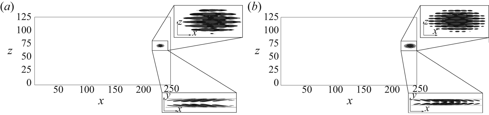
The initial optimal solutions obtained for the target time  $T = 10$ at the threshold energy able to trigger turbulence are shown in figure 2 for
 $Re=1150$. The optimal perturbation is localized spatially in a small region of the domain, with a shape similar to that of a spot, being composed of alternating positive and negative finite-size streamwise streaks. Despite spatial localization having been observed already in nonlinear optimizations (for instance, see Cherubini et al. Reference Cherubini, De Palma, Robinet and Bottaro2011; Monokrousos et al. Reference Monokrousos, Bottaro, Brandt, Di Vita and Henningson2011; Pringle et al. Reference Pringle, Willis and Kerswell2012), the structure of this optimal perturbation is rather different from that of previously computed nonlinear optimal perturbations, and more closely resembles the optimal wavepacket recovered by linear optimization and windowing, obtained for the boundary-layer flow by Cherubini et al. (Reference Cherubini, Robinet, Bottaro and De Palma2010b). This is probably due to the low target time and initial energy used for these computations, which hinders partially the development of nonlinear effects. At
 $t=0$, the optimal perturbation presents vortical structures inclined in the opposite direction with respect to the shear, which reverse their inclination at target time (see the
 $x\text {--}y$ planes in the bottom right of figures 2a,b). This streamwise tilting is a common feature of optimal perturbations in shear flows (Cherubini et al. Reference Cherubini, De Palma, Robinet and Bottaro2010a; Pringle & Kerswell Reference Pringle and Kerswell2010; Duguet et al. Reference Duguet, Monokrousos, Brandt and Henningson2013), and indicates that the Orr mechanism is a fundamental mechanism involved in the early stage of transition to turbulence, with characteristic time approximately equal to
 $10$ (Orr Reference Orr1907). Indeed, although it may seem unrealistic that perturbations inclined opposed to the mean flow can actually be observed in experiments and simulations of wall-bounded turbulent flows, recent works (Jiménez Reference Jiménez2013) have argued that such types of disturbances are in fact created in the near-wall cycle during the streak breakdown.
Nonlinear optimal perturbation at times  $t = 0$ (a) and
 $t=T = 10$ (b), for
 $Re=1150$ with the input energy
 $E_0 = 1.1 \times 10^{-7}$ (black dot in figure 1). The insets show isosurfaces of the streamwise velocity, light grey for positive and black for negative values,
 $u = \pm 0.003$ (top) and
 $u = \pm 0.02$ (bottom).

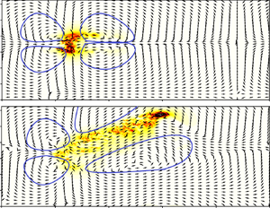
Duguet & Schlatter (Reference Duguet and Schlatter2013) show that oblique bands arise as a result of advection of newly nucleated streaks in the direction of a large-scale flow, which is oblique with respect to the streamwise direction. The local orientation of the large-scale flow is thus responsible for the obliqueness of the laminar–turbulent interface of growing incipient spots as well as for maintaining turbulent stripes (Duguet & Schlatter Reference Duguet and Schlatter2013). To ascertain whether the computed nonlinear optimal perturbations contain the seed for the development of turbulent bands, we compute the large-scale flow related to the optimal disturbances by averaging the instantaneous velocity field in the wall-normal direction as  $\overline {u_i} = \int _{-1}^{1} u_i\, {{\rm d} y}$. Notice that
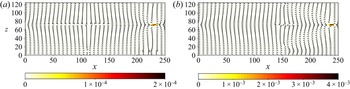
 $\bar {u}$ is zero where the flow is laminar, close to zero where the flow is turbulent, but non-zero at the laminar–turbulent interfaces, due to a mismatch of the streamwise flow rates across them, linked to the presence of overhang regions (Duguet & Schlatter Reference Duguet and Schlatter2013). Figure 3 provides the isocontours of the crossflow energy
 $E_{cf} = (1/2) \int (v^{2} +w^{2})\, {{\rm d} y}$, surrounded by the large-scale field
 $(\bar {u}, \bar {w})$, for the initial optimal perturbation at
 $Re=1150$,
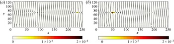
 $E_0=1.1 \times 10^{-7}$. The optimal flow field is characterized by two different scales: a small-scale flow embedded within the spot-like structure, and a large-scale flow in the form of large vortices filling the whole domain. The latter is characterized by a streamwise flow entering the spot and a spanwise flow exiting from it, constituting a quadrupolar structure. A quadrupolar large-scale flow around spots or turbulent bands has been observed in plane Couette flow (Schumacher & Eckhardt Reference Schumacher and Eckhardt2001; Lagha & Manneville Reference Lagha and Manneville2007) and plane Poiseuille flow (Lemoult et al. Reference Lemoult, Gumowski, Aider and Wesfreid2014), and very recently in the Couette–Poiseuille flow (Klotz, Pavlenko & Wesfreid Reference Klotz, Pavlenko and Wesfreid2021). This large-scale structure appears within the flow due to the shearing of the streamwise velocity and the breaking of the spanwise homogeneity (Wang et al. Reference Wang, Guet, Monchaux, Duguet and Eckhardt2020). Notice that this large-scale flow, which is not associated with the presence of overhang regions, remains almost unchanged from
 $t=0$ to
 $t=T$ (compare figures 3a,b).
Shaded isocontours of the crossflow energy  $E_{cf}$ together with the normalized
 $y$-integrated large-scale flow (vectors) characterizing the nonlinear optimal perturbations for
 $Re = 1150$,
 $E_0 = 1.1 \times 10^{-7}$,
 $T = 10$: (a) initial optimal solution,
 $t=0$; (b) optimal solution at the target time,
 $t=T$.

Increasing the target time to  $T=100$ for
 $Re=1150$, while keeping
 $E_0=1.1 \times 10^{-7}$, we obtain a similar optimal structure, characterized by a quadrupolar large-scale flow surrounding a spot-like small-scale disturbances (not shown). Starting from this optimal (but yet not minimal) solution, the optimize-and-bisect procedure is carried out with
 $T=100$ for
 $Re=1150$. The same procedure is carried out for all the considered values of
 $Re$, for obtaining the minimal seeds whose energy is reported in figure 1(b).
3.2. Minimal seed at different Reynolds numbers
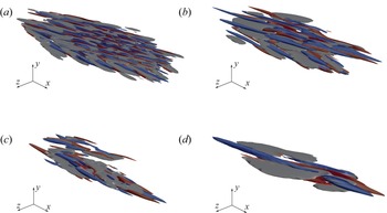
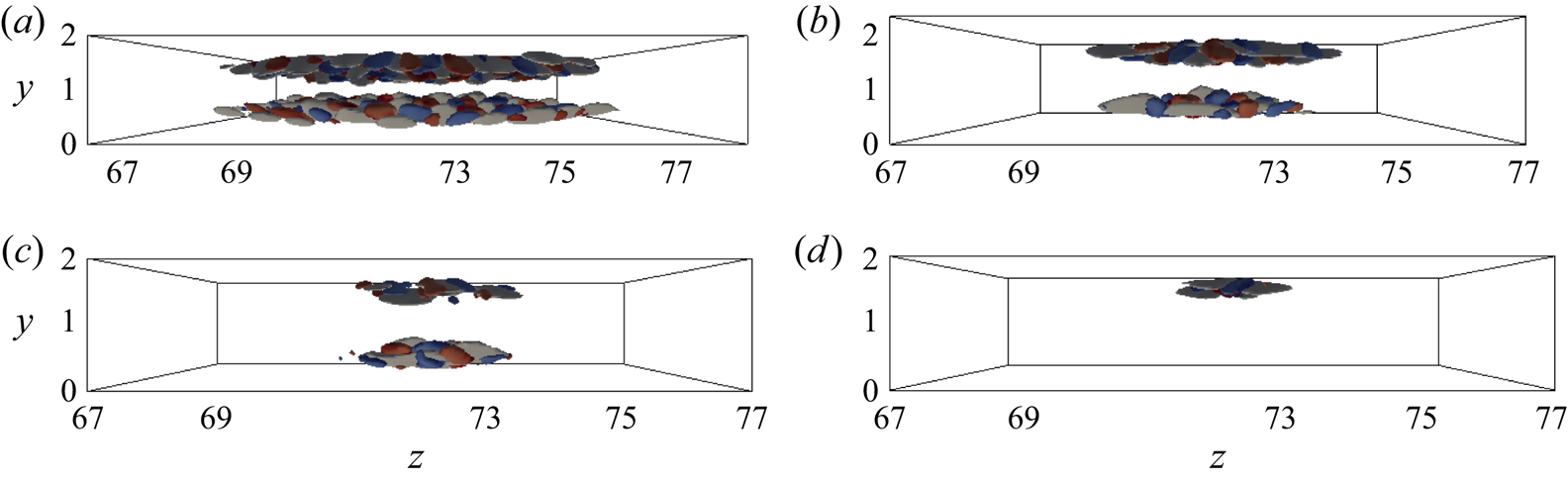
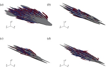
The minimal seeds for turbulent bands obtained for all the considered values of the Reynolds number are provided in figures 4 and 5 in two different views showing the streamwise and spanwise alternation of finite-size streaks together with spanwise-inclined vortical structures closer to the wall. Moreover, the large-scale flow, shown in figure 6 for  $Re=1150$, maintains the previously observed quadrupolar structure, presenting large-scale vortices quasi-symmetric in the spanwise direction. The same large-scale quadrupolar structure surrounding the minimal-energy wavepacket is observed also for the other considered Reynolds numbers (not shown). Quadrupolar structures similar to those observed around these optimal perturbations have been observed in several shear flows and spatial domains, in experiments and computations (see, for instance, Lundbladh & Johansson Reference Lundbladh and Johansson1991; Lagha & Manneville Reference Lagha and Manneville2007; Duguet & Schlatter Reference Duguet and Schlatter2013; Lemoult et al. Reference Lemoult, Aider and Wesfreid2013; Couliou & Monchaux Reference Couliou and Monchaux2015; Chantry, Tuckerman & Barkley Reference Chantry, Tuckerman and Barkley2016). This two-dimensional large-scale flow surrounding localized perturbations or turbulent spots, appears to fill out the whole domain, and shows an exponential (or algebraic) decay of its amplitude in space (see Schumacher & Eckhardt Reference Schumacher and Eckhardt2001; Brand & Gibson Reference Brand and Gibson2014). In particular, Wang et al. (Reference Wang, Guet, Monchaux, Duguet and Eckhardt2020) demonstrated that this quadrupolar structure is a generic feature of planar shear flows confined between two walls, and stems from (i) the shearing of the streamwise velocity, and (ii) the breaking of the spanwise homogeneity. The minimal seeds (and nonlinear optima) computed for all the considered Reynolds numbers show both these features, justifying the presence of these large-scale vortices. However, the small-scale minimal perturbations are found to change considerably with the Reynolds numbers, as shown in figure 4. In particular, a further localization of the initial wavepacket is observed for increasing
 $Re$, leading to a minimal structure at
 $Re=1568$ localized on only one of the two walls (see figure 4d), which resembles closely that found for the plane Couette and the asymptotic suction boundary-layer flow in small domains (Rabin et al. Reference Rabin, Caulfield and Kerswell2012; Duguet et al. Reference Duguet, Monokrousos, Brandt and Henningson2013; Cherubini et al. Reference Cherubini, De Palma and Robinet2015). Apart from the spatial localization, the main structures observed within the minimal seed wavepackets are essentially the same, namely, finite-size streaks flanking upstream-tilted elongated vortices. As a result of the discrepancies recovered at initial time, the minimal seeds obtained at different
 $Re$ evolve differently in time, presenting an increasing localization for larger values of
 $Re$, as provided in figures 7 and 8. However, all of the wavepackets present an arrow-shaped structure, with the downstream region essentially characterized by low-speed streaks, and the core region filled with small-scale vortices together with some coherent streamwise streaks. Despite having some common features with turbulent spots observed typically in transitional flows (Marxen & Zaki Reference Marxen and Zaki2019), these perturbations at target time are characterized by more coherent streaks and vortices at their head, tail and sides, and a core showing signs of streak breakdown. Moreover, the large-scale quadrupolar structure observed at
 $t=0$ is maintained at target time for all the considered values of
 $Re$, as shown in figure 6(b) for
 $Re=1150$.
Minimal seeds at different Reynolds numbers: isosurfaces of negative streamwise velocity ( $u = -0.0025$, light grey) and
 $Q$-criterion (
 $Q = 0.003$) coloured by the streamwise vorticity (positive red, negative blue). For all values of
 $Re$, only a subdomain of length
 $l_x \times \l _y \times l_z=16\times 0.5 \times 6$ is shown. Here: (a)
 $Re = 1000$,
 $E_0 = 5.5 \times 10^{-7}$; (b)
 $Re = 1150$,
 $E_0 = 4.7 \times 10^{-8}$; (c)
 $Re = 1250$,
 $E_0 = 2.9 \times 10^{-8}$; (d)
 $Re = 1568$,
 $E_0 = 3.6 \times 10^{-9}$.

Minimal seeds at different Reynolds numbers: isosurfaces of negative streamwise velocity ( $u = -0.0025$, light grey) and
 $Q$-criterion (
 $Q = 0.003$) coloured by the streamwise vorticity (positive red, negative blue). Here: (a)
 $Re = 1000$,
 $E_0 = 5.5 \times 10^{-7}$; (b)
 $Re = 1150$,
 $E_0 = 4.7 \times 10^{-8}$; (c)
 $Re = 1250$,
 $E_0 = 2.9 \times 10^{-8}$; (d)
 $Re = 1568$,
 $E_0 = 3.6 \times 10^{-9}$.

Isocontours of the crossflow energy  $E_{cf}$ with the normalized
 $y$-integrated large-scale flow (vectors) for
 $Re = 1150$,
 $E_0 = 4.7 \times 10^{-8}$,
 $T = 100$: (a) initial optimal solution,
 $t=0$; (b) optimal solution at the target time,
 $t=T$.

Minimal seeds at target time  $t = T$ for different Reynolds numbers: isosurfaces of negative streamwise velocity (
 $u = -0.03$, light grey) and
 $Q$-criterion (
 $Q = 0.005$) coloured by the streamwise vorticity (positive red, negative blue). For all values of
 $Re$, only a subdomain of length
 $l_x \times \l _y \times l_z=30\times 0.5 \times 10$ is shown. Here: (a)
 $Re = 1000$,
 $E_0 = 5.5 \times 10^{-7}$; (b)
 $Re = 1150$,
 $E_0 = 4.7 \times 10^{-8}$; (c)
 $Re = 1250$,
 $E_0 = 2.9 \times 10^{-8}$; (d)
 $Re = 1568$,
 $E_0 = 3.6 \times 10^{-9}$.

Minimal seeds at target time  $t = T$ for different Reynolds numbers: isosurfaces of negative streamwise velocity (
 $u = -0.0025$, light grey) and
 $Q$-criterion (
 $Q = 0.003$) coloured by the streamwise vorticity (positive red, negative blue). Here: (a)
 $Re = 1000$,
 $E_0 = 5.5 \times 10^{-7}$; (b)
 $Re = 1150$,
 $E_0 = 4.7 \times 10^{-8}$; (c)
 $Re = 1250$,
 $E_0 = 2.9 \times 10^{-8}$; (d)
 $Re = 1568$,
 $E_0 = 3.6 \times 10^{-9}$.

It is also interesting to compare such minimal seeds with those obtained in the previously mentioned smaller domain. A three-dimensional visualization of the small-domain minimal seeds is provided in figure 9 for the three considered Reynolds numbers. The streamwise perturbation patches alternating in the  $x$ and
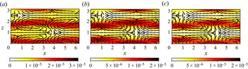
 $z$ directions are rather similar to those found for the large domain, although in the latter case this alternating structure is repeated many times in all spatial directions. Moreover, the amplitude of the small-domain minimal seeds is about twice that of the minimal perturbations obtained for the large domain, indicating that the size of the domain has a non-negligible effect on the shape, amplitude and energy of the minimal seeds. Finally, the isocontours of the crossflow energy surrounded by the large-scale field are shown in figure 10 for the small-domain minimal seeds. One can observe that a quadrupolar structure is present as well, but at a much smaller scale than in the previous case.
Minimal seeds for (a)  $Re = 1400$, (b)
 $Re = 1568$, (c)
 $Re = 1650$; isosurfaces of the streamwise velocity (light grey for positive and black for negative values,
 $u = \pm 0.005$.

Isocontours of the crossflow energy  $E_{cf}$ with the normalized
 $y$-integrated large-scale flow (vectors) for the minimal seed in the small domain for (a)
 $Re=1400$, (b)
 $Re=1568$, and (c)
 $Re=1650$.

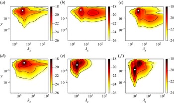
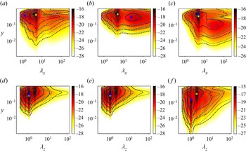
The contours of the premultiplied energy spectra of the minimal seed obtained at  $Re=1150$ are reported in figure 11. The streamwise perturbation energy peaks for
 $\lambda _z\approx 2.45$ and
 $\lambda _x\approx 3.78$ (see also table 1), whereas the wall-normal and spanwise perturbation energy have largest amplitude at
 $\lambda _z\approx 1$,
 $\lambda _x\approx 4$, with a secondary peak for
 $\lambda _z\approx 2$ and
 $\lambda _x\approx 25$. The lowest of these wavelengths are close to those reported by Lemoult et al. (Reference Lemoult, Gumowski, Aider and Wesfreid2014) concerning the development of turbulent spots at similar Reynolds numbers, and are linked to the finite size of the streaks, whereas the largest wavelengths are linked directly to the streamwise and spanwise sizes of the wavepacket. Very similar spectra are found to characterize the nonlinear optimal perturbations at higher initial energy (solid contours in figure 11). The premultiplied energy spectra of the minimal seeds obtained for the other values of
 $Re$ are reported in figure 12 by the shaded contours (
 $Re=1000$) and the dashed lines (black for
 $Re=1150$, blue for
 $Re=1250$, green for
 $Re=1568$). As a consequence of the increased spatial localization, the overall distribution of the energy spectra is displaced towards higher values of
 $\lambda _x,\lambda _z$ when
 $Re$ increases. This effect is coupled with a narrowing and displacement of the spectra towards higher values of
 $y$, which is a consequence of an increased localization also in the wall-normal direction. The peak values reported in table 1 are also influenced considerably by the Reynolds number.
Logarithm of the premultiplied spectral energy versus the wall-normal distance  $y^{+}$ for the initial optimal solution for
 $T=100$,
 $Re = 1150$, with
 $E_0 = 1.1 \times 10^{-7}$, coloured contours, and
 $E_0 = 4.7 \times 10^{-8}$, black contours. The white dots indicate the energy peaks. Here: (a)
 $\lambda _x\,E_{uu}(\lambda _x)$. (b)
 $\lambda _x\,E_{vv}(\lambda _x)$, (c)
 $\lambda _x\,E_{ww}(\lambda _x)$, (d)
 $\lambda _z\,E_{uu}(\lambda _x)$, (e)
 $\lambda _z\,E_{vv}(\lambda _x)$, (f)
 $\lambda _z\,E_{ww}(\lambda _x)$.

Logarithm of the premultiplied spectral energy versus the wall-normal distance  $y^{+}$ for the initial optimal solution at different Reynolds numbers at
 $T = 100$:
 $Re = 1000$ for
 $E_0 = 5.5 \times 10^{-7}$ (coloured contours),
 $Re = 1150$ for
 $E_0 = 4.7 \times 10^{-8}$ (black contours),
 $Re = 1250$ for
 $E_0 = 2.9 \times 10^{-8}$ (blue contours), and
 $Re = 1568$ for
 $E_0 = 5.8 \times 10^{-9}$ (green contours). The symbols indicate the peaks of the energy, also reported in table 1. Here: (a)
 $\lambda _x\,E_{uu}(\lambda _x)$, (b)
 $\lambda _x\,E_{vv}(\lambda _x)$, (c)
 $\lambda _x\,E_{ww}(\lambda _x)$, (d)
 $\lambda _z\,E_{uu}(\lambda _z)$, (e)
 $\lambda _z\,E_{vv}(\lambda _z)$, (f)
 $\lambda _z\,E_{ww}(\lambda _z)$.

Streamwise and spanwise wavelengths  $\lambda _x,\lambda _z$ associated with the primary peaks of the premultiplied energy spectra of
 $u,v,w$, shown in figure 12 for different Reynolds numbers.

3.3. Minimal seed evolution in time
In this subsection, we analyse the time evolution of the minimal seeds towards the turbulent bands. In figure 13, the time evolution of the kinetic energy, obtained from direct numerical simulations initialized with the minimal seeds, is reported. In all cases, the kinetic energy increases strongly in time until saturating towards a statistically constant value. For the lowest considered Reynolds numbers, we observe a rapid initial increase of the kinetic energy, followed by a slow phase of saturation of the energy, whereas for larger  $Re$, the initial growth is slower and leads to lower values of the kinetic energy at small time. One can notice once again that at
 $Re=1000$, the flow appears to behave rather differently from what is observed at larger Reynolds numbers. However, the minimal seeds at larger
 $Re$, despite having lower initial energy, tend towards higher values of the kinetic energy at large times, suggesting that for larger Reynolds numbers, turbulence eventually occupies a larger portion of the domain.
Time evolution of the kinetic energy for the minimal seeds obtained for the different considered Reynolds numbers.

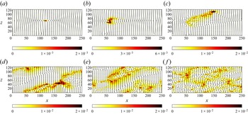
This can be verified by analysing the time evolution of the crossflow energy and  $y$-averaged flow fields for the minimal seeds at different Reynolds numbers. For
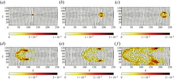
 $Re=1150$, figure 14 shows that despite its quasi-symmetric initial shape (see figure 5), the localized minimal solution breaks its symmetry rapidly along the spanwise direction. A clearly asymmetric (but still spatially compact) structure can be seen already at
 $t=500$, as shown in figure 14(b). Previous experimental and numerical works (Bullister & Orszag Reference Bullister and Orszag1987) have observed that in their initial phases, spots are more unstable in their edges, so they rapidly incur symmetry breaking. Various authors (see, for instance, Lemoult et al. Reference Lemoult, Gumowski, Aider and Wesfreid2014) have related this symmetry-breaking phase to the development of sinuous instabilities of the streaks. This asymmetric wavepacket evolves via nucleation of new streaky structures (see Parente et al. (Reference Parente, Robinet, De Palma and Cherubini2021) concerning the mechanism of creation of the streaks) in the direction of the inclined laminar–turbulent interface, clearly forming a singular turbulent band, as can be observed for
 $t = 900$. The newly formed turbulent band continues growing in an oblique direction with angle
 ${\approx }28^{\circ }$ until reaching the periodic boundaries, where it interacts with itself (
 $t=1500$). This triggers splitting of the previously isolated band (
 $t=2500$), which saturates, reaching a laminar–turbulent pattern filling the whole domain at
 $t = 4000$. The same behaviour has been observed by Tao & Xiong (Reference Tao and Xiong2013) and Xiong et al. (Reference Xiong, Tao, Chen and Brandt2015) by injecting in a plane Poiseuille flow a ‘seed’ of the turbulent bands, similar in shape to the instantaneous field at
 $t = 500$ in figure 14. Analysing the large-scale flow, we can observe the formation of a small recirculation zone upstream of the spot during its evolution. Moreover, when the bands are formed, the large-scale flow is found to turn clockwise around bands with positive angle and anticlockwise around bands with negative angle. In fact, all the bands are formed in correspondence with the shear layer that divides the different vortices. A rather similar behaviour is observed at
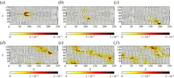
 $Re=1000$, as shown in figure 15. Despite that at small times (
 $t=150$) the minimal seed evolves into a quasi-symmetric V-shaped spot, one of its two legs weakens in time (
 $t=500$) and completely disappears at
 $t=900$, evolving into a single band, as observed for
 $Re=1150$. Whereas, looking at the evolution in time for the cases at higher Reynolds number, the flow presents the same behaviour observed experimentally and numerically when turbulence is triggered by a spot (Carlson et al. Reference Carlson, Widnall and Peeters1982; Alavyoon, Henningson & Alfredsson Reference Alavyoon, Henningson and Alfredsson1986; Henningson & Kim Reference Henningson and Kim1991; Aida et al. Reference Aida, Tsukahara and Kawaguchi2010, Reference Aida, Tsukahara and Kawaguchi2011). In fact, the localized perturbation initially evolves in the domain forming a turbulent spot, turning into a V-shape at
 $t = 500$, as shown in figure 16. At this time, two distinct fronts of the spots can be observed, which evolve in two symmetric bands with angle
 ${\approx }\pm 45^{\circ }$ growing obliquely in the domain, as shown at
 $t = 900$. At
 $t = 1200$, they start to interact with each other, forming a spatio-temporally complex final state composed of turbulent and laminar patterns (
 $t=3000$). Qualitatively, the same behaviour is observed at
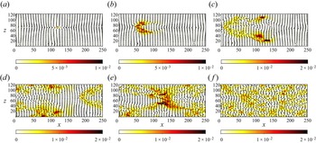
 $Re=1568$, as shown in figure 17, although the spatial spreading of the bands appears to be more rapid than at lower
 $Re$, despite the initial energy of the perturbation being lower. Also in these cases, the bands are found to be generated right in the mixing layer between two large-scale counter-rotating vortices. Notice also that the same quasi-symmetric behaviour can be observed at lower
 $Re$, for a larger initial energy. In fact, the nonlinear optimal perturbation computed for
 $Re=1150$ and
 $E_0=4.7 \times 10^{-8}>{E_0}_{min}$ evolves in two distinct bands, showing a time evolution corresponding to that of the minimal seed at largest
 $Re$ (not shown).
Isocontours of the crossflow energy  $E_{cf}$ together with the normalized
 $y$-integrated large-scale flow (vectors) for several instantaneous fields (
 $Re = 1150$,
 $E_0 = 4.7 \times 10^{-8}$,
 $T = 100$): (a)
 $t=200$, (b)
 $t=500$, (c)
 $t=900$, (d)
 $t=1500$, (e)
 $t=2500$, (f)
 $t=4000$.

Isocontours of the crossflow energy  $E_{cf}$ together with the normalized
 $y$-integrated large-scale flow for several instantaneous fields (
 $Re = 1000$,
 $E_0 = 5.5 \times 10^{-7}$,
 $T = 100$): (a)
 $t=150$, (b)
 $t=500$, (c)
 $t=900$, (d)
 $t=1500$, (e)
 $t=2500$, (f)
 $t=3000$.

Isocontours of the crossflow energy  $E_{cf}$ together with the normalized
 $y$-integrated large-scale flow for several instantaneous fields (
 $Re = 1250$,
 $E_0 = 2.9 \times 10^{-8}$,
 $T = 100$): (a)
 $t=200$, (b)
 $t=500$, (c)
 $t=900$, (d)
 $t=1200$, (e)
 $t=1500$, (f)
 $t=3000$.

Isocontours of the crossflow energy  $E_{cf}$ together with the normalized
 $y$-integrated large-scale flow for several instantaneous fields (
 $Re = 1568$,
 $E_0 = 3.6 \times 10^{-9}$,
 $T = 150$): (a)
 $t=200$, (b)
 $t=300$, (c)
 $t=350$, (d)
 $t=500$, (e)
 $t=600$, (f)
 $t=900$.

An explanation of this behaviour can be attempted by recalling that in the channel flow, turbulent stripes have a probability of decay that increases with time, and that decreases with the Reynolds number (Paranjape Reference Paranjape2019). Thus since all minimal seeds present an almost spanwise-symmetric structure, two proto-bands begin to be created at the edges of the large-scale vortices characterizing the minimal seed. However, the probability of decay of these bands is higher for low Reynolds number, and increases in time, so when  $Re$ is sufficiently low, one of these bands dies out rapidly, leading to the development of one isolated band. Increasing
 $Re$, the probability of decay of an initial band is lower, while the probability of splitting increases. Thus both oblique bands originated at the sides of the minimal seed survive longer in time, until they split and interact, leading rapidly to the establishment of a spatio-temporally complex final state. Notice that injecting more initial energy at low values of
 $Re$ has the same effect as increasing
 $Re$. In fact, an optimal perturbation with
 $E_0>{E_0}_{min}$ is less spatially localized, and is able to reach a much larger kinetic energy at
 $T=100$, leading to more spatially-extended and energetic proto-bands, which allows their sustainment for a longer time.
To corroborate this conjecture, we make use of the Reynolds–Orr equation to evaluate the production,  $P$, and dissipation,
 $\epsilon$, of kinetic energy as, respectively,
 \begin{equation} P={-}{u}_i' {u}_j'\,\frac{\partial {U}_i}{\partial x_j}, \quad \epsilon = \frac{2}{Re}\,{s_{ij}'s_{ij}'}, \quad \text{with} \ s_{ij}'=\frac{1}{2} \left(\frac{\partial {u}_i'}{\partial x_j}+\frac{\partial {u}_j'}{\partial x_i}\right), \end{equation}
where the Einstein summation convention has been used. One can compare the time evolution of the production and dissipation terms, integrated in  $x\text {--}y$ planes, for the minimal seeds at
 $Re=1150$ and
 $Re=1250$, provided in figures 18 and 19. For both Reynolds numbers, at
 $t=0$ the production presents one single peak almost in the centre of the spot (
 $z\approx 70$), which is found to exceed dissipation of almost an order of magnitude. Production of kinetic energy leads to a slight increase of the spanwise size of the wavepacket (
 $t=100$), together with a further increase of the kinetic-energy production, probably due to the nucleation of new streaks that produce kinetic energy thanks to the lift-up effect. Due to the breakdown of the structures inside the spot, dissipation increases as well, reaching almost the same value of the production term. Notice also that a weak secondary peak begins to be visible in the production term. At
 $t=500$, the spot has increased its size strongly in the spanwise direction, presenting a quasi-symmetric shape with two peaks at
 $z\approx 55\text {--}60$ and
 $z\approx 80\text {--}85$. However, at
 $t=900$, the evolution of the production and dissipation terms begins to differ strongly between the two considered Reynolds numbers. For
 $Re=1250$, the spanwise distribution of the dissipation and production terms remains quasi-spanwise-symmetric, centred at
 $z\approx 70$, with two distinct laminar–turbulent fronts at
 $z\approx 20$ and
 $z\approx 110$ (see figure 19). Whereas, for
 $Re=1150$, the leftmost part of the packet has almost faded away, while the rightmost part has expanded up to
 $z\approx 110$, as shown in figure 18. The analysis of the production and dissipation terms indicates clearly that the minimal seed for turbulent bands leads to the generation of two almost symmetric regions of high production and dissipation, which can be seen as two distinct proto-bands. However, for lower Reynolds numbers, the weaker of these two proto-bands decays rapidly, leading to the development of an isolated band, whereas at larger Reynolds numbers, both bands survive for a sufficiently long amount of time to begin self-interacting.
Spanwise distribution of the production ( $P$, red line) and dissipation (
 $-\epsilon$, black line) terms integrated in
 $x\text {--}y$ planes for different instantaneous fields obtained by evolving in time the minimal seed for
 $Re = 1150$,
 $E_0 = 4.7 \times 10^{-8}$,
 $T = 100$: (a)
 $t=0$, (b)
 $t=100$, (c)
 $t=500$, (d)
 $t=900$.

Spanwise distribution of the production ( $P$, red line) and dissipation (
 $-\epsilon$, black line) terms integrated in
 $x\text {--}y$ planes for different instantaneous fields obtained by evolving in time the minimal seed for
 $Re = 1250$,
 $E_0 = 2.9 \times 10^{-8}$,
 $T = 100$: (a)
 $t=0$, (b)
 $t=100$, (c)
 $t=500$, (d)
 $t=900$.

4. Conclusion
In this work, we have investigated the minimal-energy perturbations for the generation of turbulent bands in plane Poiseuille flow. A nonlinear optimization maximizing the kinetic energy at a given target time, coupled with initial energy bisection, has been used. The optimization was performed in very large domains, for a range of Reynolds numbers for which turbulent bands are sustained and lead to a spatio-temporally complex turbulent–laminar final state, namely  $Re = 1000$, 1150, 1250, 1568 (the lowest value being close to the threshold
 $Re$ for which bands splitting and turbulence spreading can be observed). The influence of the Reynolds number on the minimal energy threshold for generating turbulent bands (
 $E_{{0}_{min}}$) is analysed. In accordance with previous work carried out on other shear flows in small domains, the minimal seed has been found to scale with
 $Re$ following a power law
 $E_{{0}_{min}} \propto Re^{-\gamma }$, although a sufficiently good fit is found only by restraining the analysis to
 $Re>1000$. However, the value of
 $\gamma$ recovered in the present work (
 $\gamma \approx 8.5$) is approximately four times larger than the values reported in previous works (
 $\gamma \approx 2.7$ in Duguet et al. (Reference Duguet, Monokrousos, Brandt and Henningson2013),
 $\gamma \approx 2$ in Cherubini et al. (Reference Cherubini, De Palma and Robinet2015)). This may be due either to the different type of flow or to the very large domain size. Minimal seed computations carried out in a much smaller domain provided a scaling law very close to that found for the large one, although in a a limited range of
 $Re$ very close to the threshold value for observing sustained turbulence. Whereas, restraining the range of
 $Re$ to the largest values, the scaling appears to drop to
 $-3.3$, which is consistent with the values found for other shear flows. Moreover, the minimal energy threshold for transition to turbulence in the large domain is several orders of magnitude lower than that found for this smaller domain, and the structure of the minimal seeds changes as well.
For all values of the Reynolds numbers analysed, the minimal-energy perturbation able to generate turbulent bands is a spatially localized spot-like structure composed of finite-size streaks and elongated vortices. A more marked localization of the minimal seed is found when  $Re$ increases. As previously reported for the channel flow in the presence of spatially-localized spots, a large-scale flow having a quadrupolar structure has been found to surround the small-scale localized minimal perturbations. These minimal perturbations have dominant wavelengths
 ${\approx }4$ and
 ${\approx }1$ in the streamwise and spanwise directions, respectively. Nonlinear optimal perturbations, with energy higher than minimal, are characterized by similar shape and wavenumbers.
The evolution of the minimal seeds towards the turbulent bands has been investigated. For  $Re < 1250$, the minimal seeds evolve in time creating an isolated oblique band, whereas for
 $Re \geqslant 1250$, it gives rise to two distinct bands that grow quasi-symmetrically in the spanwise direction. This quasi-symmetrical evolution is observed also at lower
 $Re$ for non-minimal optimal perturbations. An analysis of the production and dissipation of kinetic energy integrated in the streamwise and wall-normal directions shows that in all cases, the initial spot-like perturbation evolves in a quasi-symmetric fashion, giving rise to two proto-bands at the edges of the large-scale flow characterizing the minimal seeds. However, since the probability of decay of the bands increases in time and is higher for low Reynolds number, when
 $Re$ is sufficiently low, one of these bands rapidly dies out, leading to the development of one isolated band. Whereas, for larger values of
 $Re$, the probability of decay of an initial band is lower, while the probability of splitting increases. Thus both oblique bands originated at the sides of the minimal seed survive for a longer time, until they split and interact, leading rapidly to the establishment of a spatio-temporally complex final state. Injecting more initial energy at low values of
 $Re$ has the same effect as increasing
 $Re$, since a more spatially extended disturbance with higher kinetic energy is reached at a small time, leading to longer and more energetic proto-bands, able to be sustained for a longer time.
This work elucidates two (apparently distinct) minimal-energy mechanisms for the generation of turbulent bands in channel flow. It appears that both the initial and final states are very sensitive to the energy and Reynolds numbers characterizing the flow, highlighting the complexity of the laminar–turbulent patterned state and its initial seed. The selection of one of these two mechanisms appears to be affected by the probability of decay of the newly created stripe, which increases with time, but decreases with the Reynolds number. Future work will aim to extend the present investigation to other shear flows presenting spatially patterned turbulence.
Funding
This work was granted access to the HPC resources of IDRIS under the allocation 2020-A0072A06362 and A0092A06362 made by GENCI.
Declaration of interests
The authors report no conflict of interest.