





Introduction
Individual vulnerability to being diagnosed with a psychiatric disorder, such as depressive disorder, is partially explained by genetic variation. In capturing this genetic liability, common variation in the human genome has recently taken center stage, with a spotlight on the development and improvement of polygenic scores (PGS). However, PGS explain only a small portion of the variance in complex traits, and many practical and ethical issues concerning their use in clinical practice are unresolved (Adeyemo et al., Reference Adeyemo, Balaconis, Darnes, Fatumo, Granados Moreno, Hodonsky, Inouye, Kanai, Kato, Knoppers, Lewis, Martin, McCarthy, Meyer, Okada, Richards, Richter, Ripatti and Rotimi2021; Murray et al., Reference Murray, Lin, Austin, McGrath, Hickie and Wray2021). In contrast, assessment of genetic liability through family history has long been established as a valuable part of medical risk assessment (Guttmacher, Collins, & Carmona, Reference Guttmacher, Collins and Carmona2004; Pyeritz, Reference Pyeritz2012; Yoon et al., Reference Yoon, Scheuner, Peterson-Oehlke, Gwinn, Faucett and Khoury2002). Family history has been linked to liability for disease, as represented by risk of diagnosis or severity-related clinical characteristics, in psychiatric disorders (Hardt & Franke, Reference Hardt and Franke2007), including common mood and anxiety disorders (Havinga et al., Reference Havinga, Boschloo, Bloemen, Nauta, de Vries, Penninx, Schoevers and Hartman2017; Hettema, Neale, & Kendler, Reference Hettema, Neale and Kendler2001; McLaughlin, Behar, & Borkovec, Reference McLaughlin, Behar and Borkovec2008; Sullivan, Neale, & Kendler, Reference Sullivan, Neale and Kendler2000). Nevertheless, the potential of family history data for prediction of psychiatric disorders has not been fully explored. For disorder prediction, it is important to optimally assess and summarize family history data. The commonly used way of enquiring about family history is to determine the presence or absence of a disorder in the (extended) family (Mars et al., Reference Mars, Lindbohm, Della Briotta Parolo, Widén, Kaprio, Palotie and Ripatti2022). More detailed, elaborate indicators can be presumed to be more informative and powerful. An example is the count of affected relatives, which can be extended with additional family-specific information, such as family size (Ali et al., Reference Ali, Sreeraj, Nadella, Holla, Mahadevan, Ithal, Balachander, Viswanath, Venkatasubramanian, John, Reddy and Jain2021; Milne et al., Reference Milne, Moffitt, Crump, Poulton, Rutter, Sears, Taylor and Caspi2008), age of relatives (van Sprang et al., Reference van Sprang, Maciejewski, Milaneschi, Elzinga, Beekman, Hartman, van Hemert and Penninx2022), age of onset in relatives (Pedersen et al., Reference Pedersen, Agerbo, Plana-Ripoll, Grove, Dreier, Musliner, Bækvad-Hansen, Athanasiadis, Schork, Bybjerg-Grauholm, Hougaard, Werge, Nordentoft, Mors, Dalsgaard, Christensen, Børglum, Mortensen, McGrath and Vilhjálmsson2022), or cohabitation (Kendler, Ohlsson, Sundquist, & Sundquist, Reference Kendler, Ohlsson, Sundquist and Sundquist2021). More elaborate indicators also make use of disorder-specific information, such as prevalence (Ruderfer, Korn, & Purcell, Reference Ruderfer, Korn and Purcell2010; van et al., Reference van Sprang, Maciejewski, Milaneschi, Elzinga, Beekman, Hartman, van Hemert and Penninx2022) and heritability (Hujoel et al., Reference Hujoel, Gazal, Loh, Patterson and Price2020; So, Kwan, Cherny, & Sham, Reference So, Kwan, Cherny and Sham2011), or cross-trait genetic correlations (Dybdahl Krebs et al., Reference Dybdahl Krebs, Georgii Hellberg, Lundberg, Appadurai, Ohlsson, Pedersen, Steinbach, Matthews, Border, LaBianca, Calle, Meijsen, Ingason, Buil, Vilhjálmsson, Flint, Bacanu, Cai, Dahl and Schork2024). Indicators further differ in the ways they are calculated, including analytical algorithms of varying complexity (So et al., Reference So, Kwan, Cherny and Sham2011; Verdoux et al., Reference Verdoux, van Os, Sham, Jones, Gilvarry and Murray1996), maximum likelihood estimation (Hujoel et al., Reference Hujoel, Gazal, Loh, Patterson and Price2020; Pedersen et al., Reference Pedersen, Agerbo, Plana-Ripoll, Grove, Dreier, Musliner, Bækvad-Hansen, Athanasiadis, Schork, Bybjerg-Grauholm, Hougaard, Werge, Nordentoft, Mors, Dalsgaard, Christensen, Børglum, Mortensen, McGrath and Vilhjálmsson2022), and step-by-step heuristics (Kendler et al., Reference Kendler, Ohlsson, Sundquist and Sundquist2021). In consequence, heterogeneous and sample-specific methodologies prohibit systematic comparison of existing results.
A comprehensive and flexible approach to summarize family history has recently been developed based on the liability threshold model (Falconer, Reference Falconer1965; So et al., Reference So, Kwan, Cherny and Sham2011). One method, the Pearson–Aitkens Family Genetic Risk Score (PAFGRS) models genetic liabilities based on family- and disease specific information, including genetic covariances. The liability of each individual is modeled as a normal distribution and updated according to their relatives’ disorder status, using a computationally cheap analytical approach (Dybdahl Krebs et al., Reference Dybdahl Krebs, Georgii Hellberg, Lundberg, Appadurai, Ohlsson, Pedersen, Steinbach, Matthews, Border, LaBianca, Calle, Meijsen, Ingason, Buil, Vilhjálmsson, Flint, Bacanu, Cai, Dahl and Schork2024). PAFGRS showed better prediction of depression than other elaborate approaches, but was not compared to simple dichotomous or proportional indicators. Additionally, its application and performance was assessed in a registry-based study, and has not yet been validated in a clinical cohort assessed with structured interviews. Here, we leveraged data from 1339 participants of the Netherlands Study of Depression and Anxiety (NESDA) (Penninx et al., Reference Penninx, Eikelenboom, Giltay, van Hemert, Riese, Schoevers and Beekman2021) to compare the performance of different genetic liability indicators in predicting lifetime depressive disorder diagnoses. We calculated simple and elaborate family history indicators from detailed interviews on family history of depression and anxiety in first-degree relatives. Our main aim was to compare different types of family history indicators in predicting depressive disorder. Furthermore, we benchmarked the prediction of the family history indicator against that of a PGS for major depression derived from the latest genome-wide association study meta-analysis (Adams et al., Reference Adams, Streit, Meng, Awasthi, Adey, Choi, Chundru, Coleman, Ferwerda, Foo, Gerring, Giannakopoulou, Gupta, Hall, Harder and McIntosh2025).
Methods
NESDA sample
The NESDA is a longitudinal cohort study aimed at investigating the course and consequences of anxiety and depressive disorders. It is described in detail elsewhere (Penninx et al., Reference Penninx, Eikelenboom, Giltay, van Hemert, Riese, Schoevers and Beekman2021). Between 2003 and 2007, participants with depressive and anxiety disorders and healthy controls were recruited from the community, primary care, and secondary care settings. Exclusion criteria were a) having a severe psychiatric disorder other than those of interest in NESDA, for example, psychotic disorders, obsessive-compulsive disorder, bipolar disorder, or addiction disorder, and b) not being fluent in Dutch. Follow-ups have taken place at intervals of 1–3 years, resulting in 6 completed waves in 2023. All participants signed informed consent and the study was approved by the Medical Ethics Committee of the participating universities.
After exclusion of closely related participants (full siblings), the final sample of the current study consisted of 1339 individuals with available family history and genotype data. Of these, 1086 participants reported a Diagnostic and Statistical Manual of Mental Disorders (DSM)-based diagnosis of depressive disorder during psychiatric interviews at one of the NESDA assessments; for 253, no depressive disorder was ascertained.
Lifetime diagnosis with depressive disorder
Lifetime diagnosis of depressive disorder (MDD or dysthymia) as defined in the DSM-IV was assessed using the Composite Interview Diagnostic Instrument (version 2.1, WHO), administered by trained research staff at baseline. By the same method, diagnostic status was updated at the 3rd, 4th, 5th, and 6th follow-up. Screened participants without any lifetime diagnosis of depressive disorder, anxiety disorder, or bipolar disorder were assigned to the control group.
Family history assessment
Family history was assessed at Wave 6 using the Family Tree Inventory interview (Fyer & Weissman, Reference Fyer and Weissman1999) in Dutch (full questionnaire see Supplementary Methods). First, each participant was asked general questions about the composition of their family. Separate questions were used to ascertain the number of biological brothers and sisters, excluding half-, step-, foster-, and adoptive siblings. Family size was calculated as the number of siblings (excluding the participant) plus two parents. Next, the existing first-degree relatives were considered one-by-one regarding basic descriptives and their likely diagnostic status.
If the presence of psychological problems was suggested for a given relative, the interviewer moved on to the specific disorder questions for depression, then anxiety. If the participant then indicated relevant symptoms, follow-up questions pertaining to whether they had accessed professional help, medication, inpatient treatment, and ECT were asked, with the purpose of increasing the reliability of self-report family diagnoses.
We compared two ways of coding the interview – here referred to as short versus extended assessment. The short assessment was based on a single core question of whether the relative had ever had an episode of depression or anxiety. For the extended assessment, relatives were classified as affected only if there was an indication that they had undergone any treatments for depression or anxiety. An illustration with the original questions can be found in Supplementary Figure S1, precise instructions in Supplementary Methods. Direct comparison of the two assessments showed only small differences in sample sizes and prevalences (see Supplementary Table S1).
The diagnosis of the family members was coded as ‘missing’ under the following conditions: (a) when the answer to the core question was missing or ‘don’t know’ and (b) when the follow up questions did not confirm diagnosis (extended assessment only). When disorder status of a family member was missing, this family member was omitted from the data, but the participant themselves was retained. We also assessed the effect of including relatives with missing data as controls instead, here referred to as imputation. This did not substantially improve sample size (Supplementary Table S2).
Given the lack of demonstrated benefit of extended assessment or imputation, the main results presented here are based exclusively on the short assessment. We conducted secondary association analyses on extended assessment and imputation.
Family history indicators
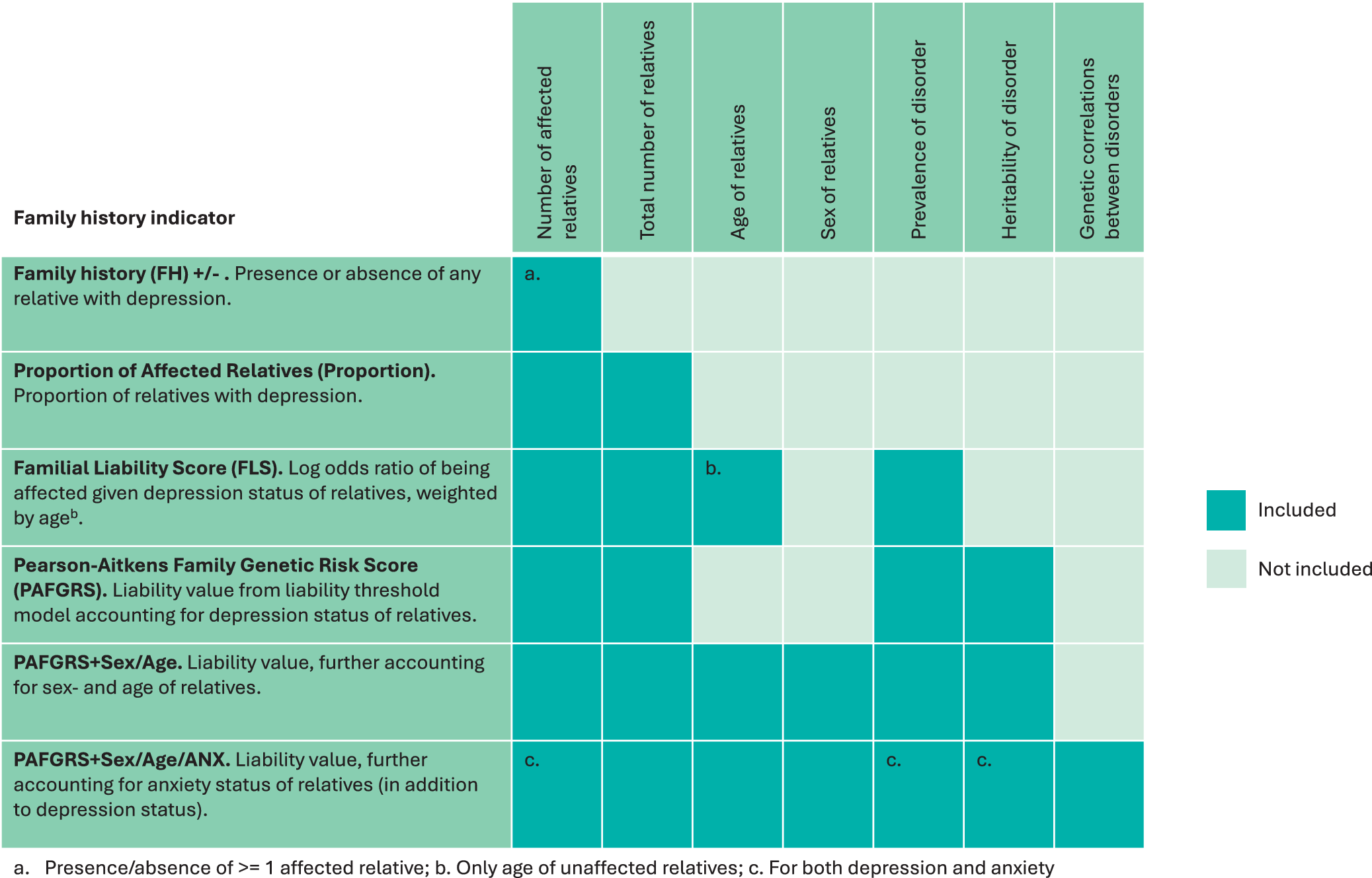
We describe below how different family history indicators were calculated in this study. Figure 1 displays the input parameters considered by each of the indicators, with reference to the example of depression.
Overview of family history indicators and their required input.

Figure 1. Long description
The table consists of seven vertical columns and six horizontal rows.
Vertical Column Headers (Inputs):
1. Number of affected relatives.
2. Total number of relatives.
3. Age of relatives.
4. Sex of relatives.
5. Prevalence of disorder.
6. Heritability of disorder.
7. Genetic correlations between disorders.
Horizontal Row Indicators (Methods):
1. Family history (F H) plus forward slash minus: Presence or absence of any relative with depression. Includes only ‘Number of affected relatives’ (marked with ‘a.’).
2. Proportion of Affected Relatives (Proportion): Proportion of relatives with depression. Includes ‘Number of affected relatives’ and ‘Total number of relatives’.
3. Familial Liability Score (F L S): Log odds ratio of being affected given depression status of relatives, weighted by age. Includes ‘Number of affected relatives’, ‘Total number of relatives’, ‘Age of relatives’ (marked with ‘b.’), and ‘Prevalence of disorder’.
4. Pearson-Aitkens Family Genetic Risk Score (P A F G R S): Liability value from liability threshold model accounting for depression status of relatives. Includes ‘Number of affected relatives’, ‘Total number of relatives’, ‘Prevalence of disorder’, and ‘Heritability of disorder’.
5. P A F G R S plus Sex forward slash Age: Liability value, further accounting for sex- and age of relatives. Includes all inputs except ‘Genetic correlations between disorders’.
6. P A F G R S plus Sex forward slash Age forward slash A N X: Liability value, further accounting for anxiety status of relatives. Includes all seven inputs. ‘Number of affected relatives’, ‘Prevalence of disorder’, and ‘Heritability of disorder’ are marked with ‘c.’.
Legend and Footnotes:
* Teal square: Included.
* Light green square: Not included.
* a. Presence forward slash absence of greater than or equal to 1 affected relative.
* b. Only age of unaffected relatives.
* c. For both depression and anxiety.
FH+/−
Family history (FH)+/− is a simple dichotomous score, indicating absence versus presence of any relatives with depression. Thus, if one or more relatives had received a diagnosis with depression, this indicator would be set to 1 (= FH+), else to 0 (= FH-).
Proportion
Proportion was calculated by dividing the number of relatives with a depression diagnosis by the total number of relatives. Thus, this indicator ranges between 0 and 1, with the number of possible levels depending on family size.
FLS
The Familial Liability Score (FLS) is a continuous indicator based on a combination of likelihood ratios per relative (Verdoux et al., Reference Verdoux, van Os, Sham, Jones, Gilvarry and Murray1996). This indicator accounts for the age of unaffected relatives, following the rationale that there is a higher certainty of low liability in individuals who have remained unaffected for a longer time. We followed the FLS algorithm as previously applied in NESDA (van et al., Reference van Sprang, Maciejewski, Milaneschi, Elzinga, Beekman, Hartman, van Hemert and Penninx2022) to depression, with the same parameters for age-of-onset range (10–65), lifetime prevalence (K) in those with affected relatives (K = 0.40), and lifetime prevalence in those without affected relatives (K = 0.094).
PAFGRS
PAFGRS is based on the liability threshold model, in which people are deemed affected when their liability exceeds a threshold. The liability is assumed to be normally distributed in the population, which defines an expected mean liability in cases and mean liability in controls. These properties are used to compute the expected genetic liability in index individuals based on disease status in relatives, while also taking into account lifetime population prevalence of the disease (Dybdahl Krebs et al., Reference Dybdahl Krebs, Georgii Hellberg, Lundberg, Appadurai, Ohlsson, Pedersen, Steinbach, Matthews, Border, LaBianca, Calle, Meijsen, Ingason, Buil, Vilhjálmsson, Flint, Bacanu, Cai, Dahl and Schork2024). Covariances and variances of genetic liabilities in the family follow from relatedness and heritability (h2). Using normal distribution theory, participants’ genetic liability was adjusted based on relatives’ liabilities to obtain a risk score. We used the R package PAFGRS (v0.1.0, [Dybdahl Krebs et al., Reference Dybdahl Krebs, Georgii Hellberg, Lundberg, Appadurai, Ohlsson, Pedersen, Steinbach, Matthews, Border, LaBianca, Calle, Meijsen, Ingason, Buil, Vilhjálmsson, Flint, Bacanu, Cai, Dahl and Schork2024]) with input of twin heritability h 2 = 0.35 (Polderman et al., Reference Polderman, Benyamin, de Leeuw, Sullivan, van Bochoven, Visscher and Posthuma2015) and lifetime prevalence K = 0.19 for depression (de Graaf, Ten Have, van Gool, & van Dorsselaer, Reference de Graaf, Ten Have, van Gool and van Dorsselaer2012).
PAFGRS+Sex/Age
PAFGRS+Sex/Age is an extension of the PAFGRS indicator that allows for a personalized prevalence estimate, based on each relative’s sex and age. This personalized prevalence estimate is accounted for by adjusting the threshold in the model described above for every family member, resulting in a more refined predictor. Sex- and age-specific prevalences were drawn from a continuous curve built from published age bin prevalences, scaled for the population prevalence of the Netherlands (de Graaf et al., Reference de Graaf, Ten Have, van Gool and van Dorsselaer2012 ; McGrath et al., Reference McGrath, Al-Hamzawi, Alonso, Altwaijri, Andrade, Bromet, Bruffaerts, de Almeida, Chardoul, Chiu, Degenhardt, Demler, Ferry, Gureje, Haro, Karam, Karam, Khaled, Kovess-Masfety and Zaslavsky2023) (Supplementary Figure S2). In relatives without age information (2.27% of relatives), we used the sex-specific average prevalence (de Graaf et al., Reference de Graaf, Ten Have, van Gool and van Dorsselaer2012). Contrary to FLS, PAFGRS+Sex/Age uses age information for both affected and unaffected relatives. The related intuition is that older age in unaffected relatives corresponds to lower liability and that younger age in affected relatives corresponds to higher liability.
PAFGRS+Sex/Age/ANX
PAFGRS+Sex/Age/ANX further extends the PAFGRS indicator, in addition to sex- and age-specific risk, with information on disease status for anxiety in relatives. The rationale is that the expected value of the genetic liability for depression is impacted by disease status for anxiety due to the genetic correlation between depression and anxiety. As such, anxiety is modeled with h 2 = 0.40 (Polderman et al., Reference Polderman, Benyamin, de Leeuw, Sullivan, van Bochoven, Visscher and Posthuma2015) and K = 0.20 (de Graaf, Ten Have, van Gool, & van Dorsselaer, Reference de Graaf, Ten Have, van Gool and van Dorsselaer2012). The effect of family history of anxiety on the liability for depression was scaled by the genetic correlation of the two disorders (rg = 0.87, (Grotzinger et al., Reference Grotzinger, Mallard, Akingbuwa, Ip, Adams, Lewis, McIntosh, Grove, Dalsgaard, Lesch, Strom, Meier, Mattheisen, Børglum, Mors, Breen and Nivard2022).
PGS
Imputed genotype data was available for 2541 NESDA participants of European Ancestry. PGS were built for these individuals based on summary statistics for major depression (Adams et al., Reference Adams, Streit, Meng, Awasthi, Adey, Choi, Chundru, Coleman, Ferwerda, Foo, Gerring, Giannakopoulou, Gupta, Hall, Harder and McIntosh2025) in European Ancestry individuals (excluding 23andMe, and the Dutch NESDA and Rotterdam study cohorts; approximately 410374 cases and 1584648 controls), using the 1000 Genomes European ancestry reference (phase 3; Auton et al. Reference Auton, Abecasis, Altshuler, Durbin, Abecasis, Bentley, Chakravarti, Clark, Donnelly, Eichler, Flicek, Gabriel, Gibbs, Green, Hurles, Knoppers, Korbel, Lander, Lee and National Eye Institute2015). PGS in the main analysis were generated using plink2 (Purcell & Chang, Reference Purcell and Chang2019) and PRS-CS (v1.1.0). PRS-CS is a Bayesian method that weighs single-nucleotide polymorphisms (SNPs) by a continuous shrinkage factor to account for LD and performs well compared to other methods (Ge et al., Reference Ge, Chen, Ni, Feng and Smoller2019). For 866,537 SNPs retained after preprocessing, posterior weights (see Supplementary Figure S3) were calculated using default hyperparameters (listed in Supplementary Methods). Secondary analyses were conducted using PGS based on the traditional Clumping and Thresholding method (PGS [C + T], Dudbridge, Reference Dudbridge2013; International Schizophrenia Consortium et al., Reference Purcell, Wray, Stone, Visscher, O’Donovan, Sullivan and Sklar2009), see Supplementary Figure S4. PGS were standardized to mean = 0 and variance = 1. Further details on imputation and preprocessing of the genotype data can be found in Supplementary Methods.
Statistical analyses
Correlations between the indicators were calculated using Pearson’s correlation; secondary analyses were based on Spearman’s rho correlation given the dichotomous nature of the FH+/− variable.
In the main confirmatory analysis, we compare predictive performance of the indicators. We conducted logistic regression of depressive disorder on all indicators separately. To assess the combined predictive performance of PAFGRS+Sex/Age/ANX and PGS, both were included in the same regression model as predictors. Individual and combined predictive performance were formally compared by conducting a –2logLikelihood test (Supplementary Table S5). Regression coefficients and p-values were inspected. Bonferroni multiple testing correction was applied in assessing statistical significance (p < 0.00625). As a parallel metric, the receiver operator curve (ROC) -- capturing the true positive rate and the false positive rate of a prediction model – was summarized as area under the curve (AUC) using the R package pROC (version 1.18.5, [Robin et al., Reference Robin, Turck, Hainard, Tiberti, Lisacek, Sanchez and Müller2011]). The main analysis was repeated adjusting for sex, age, educational attainment, and 10 population principal components.
Additionally, for illustrative purposes, we visualize incremental risk by higher score, by investigating the prediction of depressive disorder separately per quintile of PAFGRS+Sex/Age/ANX and PGS using a logistic regression model with quintile as a predictor, consequently transforming coefficients and standard errors to odds ratios and confidence intervals.
To answer our main research question, we conducted one main confirmatory analysis: Association of genetic indicators with depressive disorder, using logistic regression. Other analyses, such as mapping correlations between the indicators, were exploratory in nature.
Results
Descriptives of the NESDA sample and family history
Of the 1339 NESDA participants with available family history data and genotype data, 1086 had been diagnosed with depressive disorder at some point in their lives and 53 had never been diagnosed with a psychiatric disorder (Table 1). Participants were predominantly female (54.15% in controls, 65.47% in cases), with a mean age of 42 years. The median family size was four first-degree relatives, that is two parents and two siblings, with 50% of participants reporting between three and five first-degree relatives (one and three siblings). Across indicators, the mean familial risk for depression was larger in cases than controls, with similar variance in the two groups.
Sample characteristics

Table 1. Long description
The table is divided into two main sections: Sample characteristics and Family history indicators for depression.
Sample characteristics:
* N: 253 for Controls; 1086 for Depressive disorder cases.
* Age (Mean [S D]): 43.00 [14.24] for Controls; 42.46 [12.60] for Cases.
* Sex (percent female): 54.15 for Controls; 65.47 for Cases.
* Number of 1st-degree relatives (Median [I Q R; Range]): 4 [3–5; 2–14] for Controls; 4 [3–5; 2–17] for Cases.
Family history indicators for depression:
* F H plus / minus (percent F H plus): 44.27 for Controls; 68.6 for Cases.
* Proportion (Mean [S D]): 0.16 [0.24] for Controls; 0.32 [0.35] for Cases.
* F L S (Mean [S D]): minus 0.11 [0.63] for Controls; 0.25 [0.72] for Cases.
* P A F G R S (Mean [S D]): minus 0.03 [0.24] for Controls; 0.14 [0.28] for Cases.
* P A F G R S plus Sex / Age (Mean [S D]): minus 0.03 [0.24] for Controls; 0.15 [0.29] for Cases.
* P A F G R S plus Sex / Age / A N X (Mean [S D]): minus 0.10 [0.24] for Controls; 0.10 [0.28] for Cases.
* P G S (Mean [S D]): minus 0.31 [1.02] for Controls; 0.05 [1.00] for Cases. P G S was standardized to mean 0 and S D 1 in the full sample.
Note: Dep., depressive disorder; SD, standard deviation; IQR, inter-quartile range; FH+/−, family history of depression present/absent; FH+, family history of depression present; FLS, familial liability score; PAFGRS, Pearson–Aitkens Family Genetic Risk Score; PAFGRS + Sex/Age, PAFGRS based on disorder prevalence at relatives’ age and sex; PAFGRS + Sex/Age/ANX, PAFGRS based on disorder prevalence at relatives’ age and sex, and considering relatives’ anxiety status; PGS, polygenic score.
a PGS was standardized to mean = 0 and sd = 1 in full sample.
Distributions of both family history indicators and PGS show a distinction between depressive disorder cases and controls, with higher levels in cases (Figure 2). Peaks in family history indicator density plots correspond to the number of affected individuals in families of different sizes (apart from the dichotomous FH+/−). By definition, PGS are normally distributed.
Density plots of family history indicators by depressive disorder. Note: Dep., depressive disorder; FH+, family history of depression present; FLS, familial liability score; PAFGRS, Pearson–Aitkens Family Genetic Risk Score; PAFGRS + Sex/Age, PAFGRS based on disorder prevalence at relatives’ age and sex; PAFGRS + Sex/Age/ANX, PAFGRS based on disorder prevalence at relatives’ age and sex, and considering relatives’ anxiety status; PGS, Polygenic Score.

Figure 2. Long description
The figure consists of seven panels arranged in two rows. A legend on the right indicates dark blue for Controls and light green for Dep. Cases.
Top Row:
* Panel 1: A bar chart showing the Proportion of F H plus. Controls (0) have a proportion of approximately 0.45, while Dep. Cases (1) have a higher proportion of approximately 0.70.
* Panel 2: A density plot of Proportion. Both groups show a sharp peak at 0.00, with Dep. Cases showing slightly higher density in the 0.25 to 0.75 range.
* Panel 3: A density plot of F L S. Both groups show multimodal distributions centered around 0, with Dep. Cases showing a higher peak near 0.5.
Bottom Row:
* Panel 4: A density plot of P A F G R S. Both groups show a primary peak near negative 0.2, but Dep. Cases have significantly higher density in the positive range from 0.0 to 0.75.
* Panel 5: A density plot of P A F G R S plus Sex forward slash Age. The distribution is similar to Panel 4, with Dep. Cases showing a distinct rightward shift and higher density in positive risk scores.
* Panel 6: A density plot of P A F G R S plus Sex forward slash Age forward slash A N X. The trend remains consistent with the previous two panels, showing higher familial risk density for Dep. Cases.
* Panel 7: A density plot of P G S. Both groups show a normal bell-shaped curve centered near 0, with Dep. Cases showing a very slight rightward shift compared to Controls.
Relationship between family history indicators and PGS
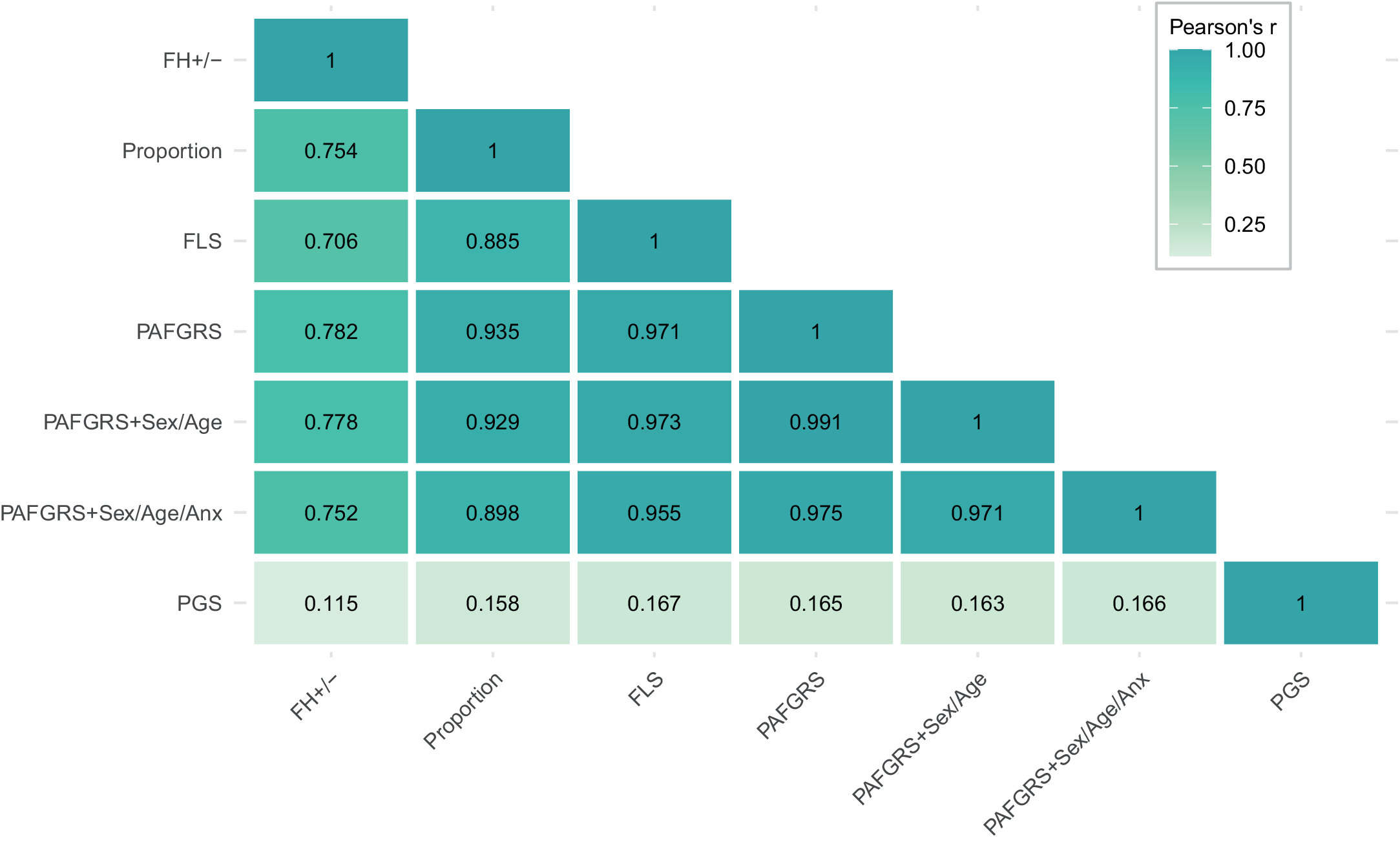
The family history indicators were highly correlated but not identical (Figure 3). Correlations between the continuous family history indicators (Proportion, FLS, PAFGRS, PAFGRS+Sex/Age, PAFGRS+Sex/Age/ANX) were particularly high, ranging from r = 0.885 to r = 0.991. Specifically, the three PAFGRS scores were highly correlated to each other (0.971–0.991), the FLS score (0.955–0.973), and the proportion score (0.898–0.935). FH+/− was slightly less correlated to the other indicators (r = 0.706–0.782), due to ignoring detailed family history information and as a statistical consequence of contrasting a dichotomous indicator to a non-dichotomous indicator. In contrast, correlations between the PGS and the family history indicators were small (r = 0.115–0.167). The presented results are based on Pearson correlation estimations; Spearman’s rank correlations show a similar pattern (Supplementary Figure S5).
Pearson correlations between family history indicators and PGS. Note: FH+/−, family history of depression present/absent; FLS, familial liability score; PAFGRS, Pearson–Aitkens Family Genetic Risk Score; PAFGRS + Sex/Age, PAFGRS based on disorder prevalence at relatives’ age and sex; PAFGRS + Sex/Age/ANX, PAFGRS based on disorder prevalence at relatives’ age and sex, and considering relatives’ anxiety status; PGS, Polygenic Score.

Figure 3. Long description
A heatmap with a color scale for Pearson’s r ranging from light green (0.25) to dark teal (1.00). The vertical axis lists seven variables from top to bottom, which are mirrored on the horizontal axis from left to right: F H plus or minus, Proportion, F L S, P A F G R S, P A F G R S plus Sex forward slash Age, P A F G R S plus Sex forward slash Age forward slash Anx, and P G S.
Data points by row:
* Row 1: F H plus or minus correlates with itself at 1.
* Row 2: Proportion correlates with F H plus or minus at 0.754 and itself at 1.
* Row 3: F L S correlates with F H plus or minus at 0.706, Proportion at 0.885, and itself at 1.
* Row 4: P A F G R S correlates with F H plus or minus at 0.782, Proportion at 0.935, F L S at 0.971, and itself at 1.
* Row 5: P A F G R S plus Sex forward slash Age correlates with F H plus or minus at 0.778, Proportion at 0.929, F L S at 0.973, P A F G R S at 0.991, and itself at 1.
* Row 6: P A F G R S plus Sex forward slash Age forward slash Anx correlates with F H plus or minus at 0.752, Proportion at 0.898, F L S at 0.955, P A F G R S at 0.975, P A F G R S plus Sex forward slash Age at 0.971, and itself at 1.
* Row 7: P G S shows the lowest correlations, ranging from 0.115 with F H plus or minus to 0.167 with F L S, and correlates with itself at 1.
Prediction of depressive disorder by family history indicators and PGS
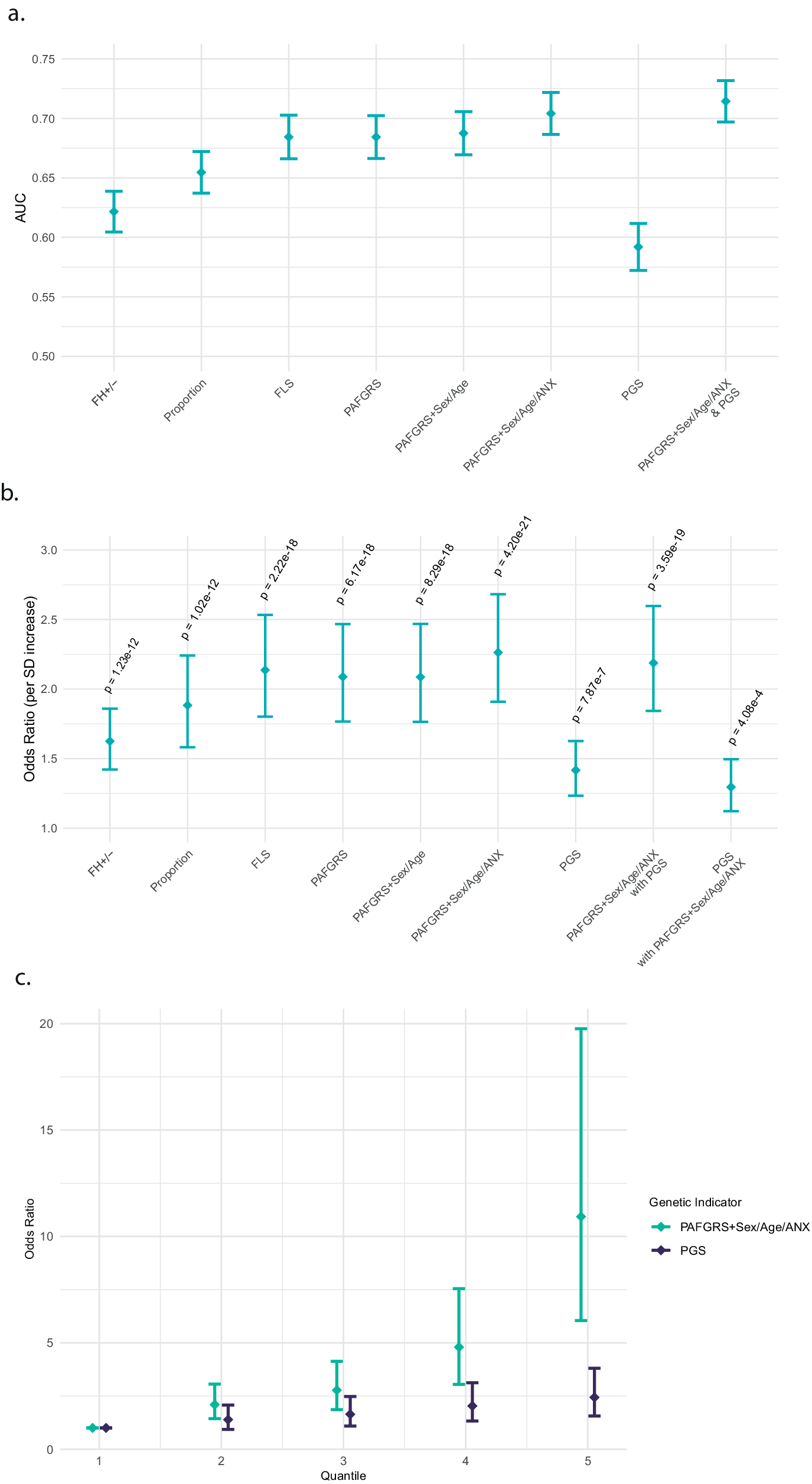
Associations of genetic indicators with depressive disorder were significant at Bonferroni-adjusted p < 0.0065 across predictors (Figure 4a,b, Supplementary Table S3). Predictive results for extended assessment and imputation can be found in Supplementary Figure S6. Overall, predictive accuracy was moderate, ranging from an AUC of 0.59 to 0.71. The predictive accuracy of the more complete family history indicators FLS (AUC = 0.68) and PAFGRS (AUC = 0.68, 0.69, 0.70) was slightly greater than that of the less complete indicators like FH = +/− (AUC = 0.62) and Proportion (AUC = 0.65), albeit with overlapping confidence intervals. As expected, the predictive accuracy of the PGS was lower than that of all family history indicators (AUC = 0.59). Adding the PGS to the best-performing family history indicator (PAFGRS+Sex/Age/ANX) slightly increased predictive accuracy (AUC = 0.71), albeit with overlapping confidence intervals. Regression coefficients were attenuated compared to a univariate model (Supplementary Table S3). A -2logLikelihood test indicated a statistically significant difference in model fit (PGS versus Combined: Chisq = 94.32, p < 2.2e-16; PAFGRS+Sex/Age/ANX versus Combined: Chisq = 12.68, p = 3.69e-4), potentially suggesting that family history and PGS are complementary in predicting depressive disorder.
Results of logistic regression model predicting depressive disorder from genetic indicator(s). Note: PAFGRS, Pearson–Aitkens Family Genetic Risk Score; PAFGRS + Sex/Age, PAFGRS based on disorder prevalence at relatives’ age and sex; PAFGRS + Sex/Age/ANX, PAFGRS based on disorder prevalence at relatives’ age and sex, and considering relatives’ anxiety status; PGS, Polygenic Score. (a) AUC of logistic regression model. FH+/−, Family history of depression present/absent; FLS, Familial Liability Score; AUC, Area under the curve; P, p-value of the regression coefficient for the respective family history indicator; in combined model of family history and PGS, P(FH), p-value for PAFGRS+Sex/Age/ANX; P(PGS), p-value for PGS. For full results, see Supplementary Table S3. (b) Odds ratios of logistic regression model. FH+/−, Family history of depression present/absent; FLS, Familial Liability Score; SD, standard deviation. Error bars represent 95% confidence intervals. For full results, see Supplementary Table S3. (c) Odds ratios for depression in PAFGRS + Sex/Age/ANX and PGS by quintile. Error bars represent 95% confidence intervals. Due to low sample size, we chose to divide the sample into quintiles; we note that this results in less pronounced odds ratios compared to dividing into deciles, as in e.g. Adams et al., Reference Adams, Streit, Meng, Awasthi, Adey, Choi, Chundru, Coleman, Ferwerda, Foo, Gerring, Giannakopoulou, Gupta, Hall, Harder and McIntosh2025.

Figure 4. Long description
Panel a is a dot plot showing A U C values on the y-axis from 0.50 to 0.75. From left to right, indicators include F H plus or minus, Proportion, F L S, P A F G R S, P A F G R S plus Sex forward slash Age, P A F G R S plus Sex forward slash Age forward slash A N X, P G S, and a combined model. A U C values generally increase from 0.62 for F H plus or minus to approximately 0.72 for the combined model, with P G S alone being the lowest at approximately 0.59.
Panel b shows Odds Ratios per S D increase on a y-axis from 1.0 to 3.0. The indicators follow the same order as panel a. Odds ratios range from approximately 1.4 for P G S to 2.3 for P A F G R S plus Sex forward slash Age forward slash A N X. Each point includes vertical error bars for 95 percent confidence intervals and an associated p-value label above it, such as p equals 4.20e minus 21 for the highest performing single indicator.
Panel c is a line and point graph showing Odds Ratios on the y-axis from 0 to 20 across five Quantiles on the x-axis. It compares two indicators: P A F G R S plus Sex forward slash Age forward slash A N X in teal and P G S in dark purple. For P G S, the odds ratio increases slightly from 1.0 at quantile 1 to approximately 2.5 at quantile 5. For the P A F G R S indicator, the increase is exponential, starting at 1.0 at quantile 1 and rising sharply to an odds ratio of approximately 11.0 at quantile 5, with a very wide confidence interval extending to nearly 20.
Similar results were found for PGS (C + T), see Supplementary Figure S7. All results remained highly similar after adjusting for covariates, for example, PAFGRS+Sex/Age/ANX: main model OR (95%CI) = 2.26 (1.91–2.68); covariate-adjusted model OR (95% CI) = 2.41 (2.01–2.9). Statistical significance of individual associations did not change; see Supplementary Table S3.
Further detailing the relationship with depressive disorder, there was a clear trend that those in higher quantiles of family history and PGS have a higher risk for depression (Figure 4c). The family history indicator shows a stronger relationship with depressive disorder than the PGS, as expected from its greater AUC (Figure 4a). This was particularly noticeable in the fifth quantile, that is the 20% of persons with the greatest liability. We note that the estimates in larger quantiles show increasing confidence intervals, which is primarily due to nonlinear scaling from the log odds scale to the OR scale, and partly due to the fifth quantile having a less-balanced case control ratio (resulting in a minimum of N = 14 controls for PAFGRS+Sex/Age/ANX; see Supplementary Table S4).
Discussion
We directly compared a range of elaborate family history indicators to each other regarding their prediction of depressive disorder in a large clinical cohort study with established psychiatric diagnoses, and by including simple and convenient indicators such as dichotomous and proportion scores.
We found high correlations between the family history indicators, with a tendency for scores based on more types of input and more precise methods to be more predictive. Analysis alongside a polygenic score indicated that family history and genotypic data contain complementary information such that combining the two can improve prediction.
Patterns of associations between genetic indicators were in line with expectations and previous literature, providing important context for our prediction models. The correlations between continuous family history indicators were particularly high (>0.88). We thus extend the previous findings of high correlations between elaborate family history indicators (Dybdahl Krebs et al., Reference Dybdahl Krebs, Georgii Hellberg, Lundberg, Appadurai, Ohlsson, Pedersen, Steinbach, Matthews, Border, LaBianca, Calle, Meijsen, Ingason, Buil, Vilhjálmsson, Flint, Bacanu, Cai, Dahl and Schork2024) by highlighting that – in a clinical cohort with self-reported family history – a simpler continuous indicator – such as the proportion of family members affected – is also highly correlated with more complex scores.
More elaborate indicators were found to be slightly more predictive of depressive disorder, suggesting that added information on family size, sex and age of relatives, disorder prevalence, and heritability do capture relevant signal rather than noise. The dichotomous indicator showed the lowest predictive accuracy, in line with previous findings (Milne et al., Reference Milne, Moffitt, Crump, Poulton, Rutter, Sears, Taylor and Caspi2008). Differences between elaborate disorder-informed indicators were not significant, which may be attributable to the relatively small NESDA sample and assessment of first-degree relatives only. When selecting a family history indicator for research or clinical practice, practical applicability of methods becomes important. Challenges faced by older non-genetic elaborate scores include (a) the treatment of missing data, (b) considering age at risk, and (c) considering co-occurring disorders (Ali et al., Reference Ali, Sreeraj, Nadella, Holla, Mahadevan, Ithal, Balachander, Viswanath, Venkatasubramanian, John, Reddy and Jain2021). All of these are solved by novel methods like PAFGRS, which offers a theoretically neat way of expanding the modeled liability with available data on (a)–(c). The PAFGRS method also flaunts inherent usability and transferability across datasets. Overall, our results suggest that elaborate family history indicators are best suited to predict depression status, with PAFGRS additionally benefiting from the theoretical and practical advantages of modeling risk on the liability scale.
Across family history indicators, predictive accuracy was limited (AUC 0.62–0.70). However, even ideal genetic indicators are limited in explanatory power (Baselmans, Yengo, van Rheenen, & Wray, Reference Baselmans, Yengo, van Rheenen and Wray2021) by the outcome trait’s heritability (depression: h2Twin = 0.35 (Polderman et al., Reference Polderman, Benyamin, de Leeuw, Sullivan, van Bochoven, Visscher and Posthuma2015), h2SNP = 8.4% (Adams et al., Reference Adams, Streit, Meng, Awasthi, Adey, Choi, Chundru, Coleman, Ferwerda, Foo, Gerring, Giannakopoulou, Gupta, Hall, Harder and McIntosh2025). Additionally, benchmarking family history indicators against the PGS highlighted the predictive value of family history.
The limited performance of the PGS may in part reflect lower predictive performance in NESDA (with null = 0.037) compared to other studies (null = 0.058 averaged across 42 European cohorts in Adams et al., Reference Adams, Streit, Meng, Awasthi, Adey, Choi, Chundru, Coleman, Ferwerda, Foo, Gerring, Giannakopoulou, Gupta, Hall, Harder and McIntosh2025). Nevertheless, PGS predictive accuracy (AUC 0.58) was in line with results from Dybdahl Krebs et al. (Reference Dybdahl Krebs, Georgii Hellberg, Lundberg, Appadurai, Ohlsson, Pedersen, Steinbach, Matthews, Border, LaBianca, Calle, Meijsen, Ingason, Buil, Vilhjálmsson, Flint, Bacanu, Cai, Dahl and Schork2024) (AUC 0.59), whereas PAFGRS predictive accuracy was slightly higher in our study (AUC 0.68–0.70) compared to the previous study (AUC 0.60–0.62). We hypothesize that this difference may be attributable to more severe and more accurately classified cases in the clinical NESDA cohort.
Both the divergence in predictive accuracy and the low correlations between family history indicators and PGS (0.11–0.16) are explained by the different aspects of genetic liability they capture. Firstly, PGS are still based exclusively on common genetic variants whose effects are inevitably estimated with noise. The precision of PGS in our study may, for instance, be affected by the genetic correlation between depression in the discovery GWAS (with assessment ranging from self-report to clinical diagnosis) and depression in NESDA being smaller than 1 (NESDA does not have the sample size to test this adequately). Secondly, even if SNP effects could have been assessed with full precision, the gap between SNP-heritability and family-based heritability has been well described (Matthews & Turkheimer, Reference Matthews and Turkheimer2022) and may be attributable to family history capturing other causes of genetic variation, such as rare variants, gene–gene interactions, or indirect genetic effects via parental genotypes. Third, inclusion of shared environmental effects (c 2 < = 0.1) in family history indicators can reduce its correlation with the PGS (Dybdahl Krebs et al., Reference Dybdahl Krebs, Appadurai, Georgii Hellberg, Ohlsson, Steinbach, Pedersen, Werge, Sundquist, Sundquist, Border, Cai, Zaitlen, Dahl, Vilhjalmsson, Flint, Bacanu, Kendler and Schork2026). Although shared environmental effects are generally viewed as negligible in the field of behavioral genetics (Plomin, DeFries, Knopik, & Neiderhiser, Reference Plomin, DeFries, Knopik and Neiderhiser2016), moderate influences can be detected for psychiatric phenotypes (Burt, Reference Burt2009; Polderman et al., Reference Polderman, Benyamin, de Leeuw, Sullivan, van Bochoven, Visscher and Posthuma2015). Shared environmental effects may be moderated by cohabitation (Kendler et al., Reference Kendler, Ohlsson, Sundquist and Sundquist2021) or other familial circumstances such as parental divorce, which we were not able to take into account in the present study.
In contrast to our results predicting depressive disorder (prevalence 0.2), lower predictive accuracy of family history is expected in rare disorders, as absence of affected family members in many families may lead to insufficient differentiation. Indeed, simulations have shown that family history indicators generally perform well in common disorders, whereas SNP-based scores perform better in rare diseases (Do, Hinds, Francke, & Eriksson, Reference Do, Hinds, Francke and Eriksson2012; So et al., Reference So, Kwan, Cherny and Sham2011). Additionally, Dybdahl Krebs et al. (Reference Dybdahl Krebs, Georgii Hellberg, Lundberg, Appadurai, Ohlsson, Pedersen, Steinbach, Matthews, Border, LaBianca, Calle, Meijsen, Ingason, Buil, Vilhjálmsson, Flint, Bacanu, Cai, Dahl and Schork2024) demonstrated that the correlation between PAFGRS and PGS is a function of the modeled trait’s heritability, prevalence, and training GWAS used for the PGS. Training GWAS sample size (Adams et al., Reference Adams, Streit, Meng, Awasthi, Adey, Choi, Chundru, Coleman, Ferwerda, Foo, Gerring, Giannakopoulou, Gupta, Hall, Harder and McIntosh2025; Howard et al., Reference Howard, Adams, Clarke, Hafferty, Gibson, Shirali, Coleman, Hagenaars, Ward, Wigmore, Alloza, Shen, Barbu, Xu, Whalley, Marioni, Porteous, Davies, Deary and … McIntosh2019) may be an explanation for the current results slightly exceeding correlations between PGS and PAFGRS observed in the iPsych Biobank (0.072–0.079, [Dybdahl Krebs et al., Reference Dybdahl Krebs, Appadurai, Georgii Hellberg, Ohlsson, Steinbach, Pedersen, Werge, Sundquist, Sundquist, Border, Cai, Zaitlen, Dahl, Vilhjalmsson, Flint, Bacanu, Kendler and Schork2026]).
We found that although PAFGRS and PGS were both associated with depressive disorders, they still captured partially independent portions of disease liability, as indicated by the limited attenuation of their individual statistically significant associations when they were jointly modeled. This highlights the added value of including both family history and polygenic scores in prediction models. Simulations have shown that family history and SNP-based indicators are likely to remain complementary in the near future, with family history proving especially valuable in more common traits and when training GWAS for the PGS are smaller (Dybdahl Krebs et al., Reference Dybdahl Krebs, Appadurai, Georgii Hellberg, Ohlsson, Steinbach, Pedersen, Werge, Sundquist, Sundquist, Border, Cai, Zaitlen, Dahl, Vilhjalmsson, Flint, Bacanu, Kendler and Schork2026). Previous studies have successfully combined genotype and family history (albeit often dichotomous), for instance, improving prediction of schizophrenia (Lu et al., Reference Lu, Pouget, Andreassen, Djurovic, Esko, Hultman, Metspalu, Milani, Werge and Sullivan2017; Lu, Forgetta, Richards, & Greenwood, Reference Lu, Forgetta, Richards and Greenwood2022) and obesity (Wang et al., Reference Wang, Hartman, Study, Visscher and Snieder2025). Family history data has also been included into molecular genetics studies to optimize the power of genome-wide association studies (Hujoel et al., Reference Hujoel, Gazal, Loh, Patterson and Price2020; Liu, Erlich, & Pickrell, Reference Liu, Erlich and Pickrell2017; Pedersen et al., Reference Pedersen, Agerbo, Plana-Ripoll, Grove, Dreier, Musliner, Bækvad-Hansen, Athanasiadis, Schork, Bybjerg-Grauholm, Hougaard, Werge, Nordentoft, Mors, Dalsgaard, Christensen, Børglum, Mortensen, McGrath and Vilhjálmsson2022). Comparison between family- and genotype-derived measures remains an area for further research investigating cutting-edge elaborate indicators and diverse disease phenotypes.
Limitations
Our study is subject to a number of limitations. First, for comparing predictors with relatively small differences in prediction accuracy, the available sample had suboptimal power. However, the NESDA sample benefits from deep phenotyping with clinically validated depressive disorder assessment and detailed family history assessment. Second, the case–control ratio in NESDA is unbalanced (81% cases), as recruitment focused on patients with clinical depression or anxiety, which could lead to sub-optimal power. Nevertheless, we were able to detect statistically significant associations between genetic risk predictors and depression diagnostic status. Additionally, we note that the AUC metric is robust to oversampling of cases (Hand & Till, Reference Hand and Till2001). Third, the family history data was based on retrospective self-report, which – in contrast to registry-based studies – may be subject to recall bias. Recall bias may result in under-reporting by controls (Weissman, Reference Weissman1987) and over-reporting by cases (Heun, Maier, & Müller, Reference Heun, Maier and Müller1997). However, analysis of validation questions -- referring for instance to medication use – did not change results (Supplementary Figure S4), suggesting that the impact of recall bias may have been limited. Importantly, self-report assessment is also reflective of realistic clinical settings; for example, the Dutch healthcare system. Fourth, including only first-degree relatives leads to relatively small families, at a cost to the accuracy of family history information. Such small pedigrees may yield less power compared to also including second- and third-degree relatives (Do, Hinds, Francke, & Eriksson, Reference Do, Hinds, Francke and Eriksson2012). However, reports about second-degree relatives are expected to be less informative for prediction due to the smaller genetic relationship, may be subject to greater measurement error, and would be harder to assess in clinical practice. Fifth, age of onset in affected relatives is unknown in our sample, which may constitute a lack of information that could have been used to improve prediction. However, in the PAFGRS model, its impact can to some extent be compensated by modeling age at interview.
Conclusion
We conclude that elaborate family history indicators are better suited to predict depressive disorder. Our study extends previous findings to new data, specifically self-report in a clinical cohort which reflects a realistic clinical scenario. In addition, we showed that family history complements genotypic scores in the prediction of lifetime depression, providing insights relevant to both research and clinical practice.
Supplementary material
The supplementary material for this article can be found at http://doi.org/10.1017/S0033291726106151.
Data availability statement
The main scripts used for preprocessing and analysis of the data are available through GitHub (https://github.com/EmmaPru/family-history-NESDA).
Author contribution
Conceptualization: E.P. and W.P.; Data Curation: E.P.; Formal analysis: E.P. and P.B.; Funding acquisition: B.W.J.H.P.; Methodology: EP and WP.; Writing – Original Draft: E.P. and W.P.; Writing – Review and Editing: All authors.
Funding statement
EP, BWJHP, WJP, and MB are supported by Stress in Action (NWO gravitation grant number 024.005.010). YM is supported by EU H2020 TO_AITION (grant number: 848146), Amsterdam UMC (Starter Grant Ronde 2), Amsterdam Neuroscience (PoC funding 2024–2026), and the ImmunoMIND consortium, funded by UK Research & Innovation as part of the UK national Mental Health Platform. The work of WJP was financially partly supported by the Amsterdam Cohort Hub, which is part of the Sector Plan ‘Accelerating Health’ of the Dutch Ministry of Education, Culture and Science.
The infrastructure for the NESDA study (www.nesda.nl) is funded through the Geestkracht program of the Netherlands Organisation for Health Research and Development (ZonMw, grant number 10-000-1002) and financial contributions by participating universities and mental healthcare organizations (Amsterdam University Medical Centers [location VUmc], GGZ inGeest, Leiden University Medical Center, Leiden University, GGZ Rivierduinen, University Medical Center Groningen, University of Groningen, Lentis, GGZ Friesland, GGZ Drenthe, and Rob Giel Onderzoekcentrum). Open access funding provided by Amsterdam UMC Location VUmc.
Competing interests
The authors declare no biomedical financial interests or potential conflicts of interest.




 Open access

