


Impact Statement
In the face of climate change, studying stream water warming is of critical importance. Existing models span a wide range, from data-driven approaches that ignore riparian vegetation to highly complex physical models that underutilize remote and in-situ sensor data. Recent advances in satellite remote sensing and machine learning have opened new possibilities for modeling water temperature, enabling spatially explicit characterization of vegetation and its nonlinear interactions with climatic and topographic factors. This work presents a data-driven modeling approach leveraging a Gaussian Attention Layer-based neural network that integrates remote and in-situ data with riparian vegetation information to predict stream water temperature. The resulting models are both interpretable and achieve state-of-the-art performance.
1. Introduction
Rivers are dynamic systems whose thermal regimes influence dissolved oxygen, metabolic rates, species phenology, and habitat suitability. Even modest increases in water temperature can disproportionately stress cold-water ecosystems and, in particular, some taxa such as salmonids (Elliott and Elliott, Reference Elliott and Elliott2010; Jackson et al., Reference Jackson, Fryer, Hannah, Millar and Malcolm2018; Feigl et al., Reference Feigl, Lebiedzinski, Herrnegger and Schulz2021; Johnson et al., Reference Johnson, Albertson, Algar, Dugdale, Edwards, England, Gibbins, Kazama, Komori, MacColl, Scholl, Wilby, de and Wood2024). Across Europe and particularly in Switzerland, warming trends in stream and river temperatures have been documented over recent decades, driven by rising air temperatures and altered hydrological regimes (Michel et al., Reference Michel, Brauchli, Lehning, Schaefli and Huwald2020; Mohsen et al., Reference Mohsen, Kiss, Baranya, Balla and Kovács2024).
Building on a long history of stream temperature research (Ouellet et al., Reference Ouellet, St-Hilaire, Dugdale, Hannah, Krause and Proulx-Ouellet2020), modeling frameworks have evolved from early empirical and energy-balance approaches (Raphael, Reference Raphael1962; Vannote and Sweeney, Reference Vannote and Sweeney1980) to more detailed process-based models representing heat exchanges between the atmosphere, channel, and surrounding environment (Caissie, Reference Caissie2006). These models progressively accounted for spatial and temporal variability in meteorological, hydrological, and landscape controls (Carrivick et al. Reference Carrivick, Brown, Hannah and Turner2012), while recent advances incorporate high-resolution remote sensing and machine-learning methods to capture nonlinear interactions and fine-scale influences (Zhu and Piotrowski, Reference Zhu and Piotrowski2020). Our framework builds on this tradition by integrating spatially explicit riparian vegetation metrics with meteorological predictors in a data-driven model.
At regional scales, stream water temperature is often closely linked to meteorological drivers such as air temperature. However, local and reach-scale deviations frequently arise from riparian vegetation, which shades streams, moderates microclimate, influences near-bank turbulence, and reduces solar heat fluxes to the water surface (Garner et al., Reference Garner, Malcolm, Sadler and Hannah2017; Kalny et al., Reference Kalny, Laaha, Melcher, Trimmel, Rauch and Schmutz2017; Dugdale et al., Reference Dugdale, Malcolm, Kantola and Hannah2018). Empirical studies have quantified substantial temperature differences between shaded and exposed reaches, with variations of several degrees Celsius observed in pre-Alpine systems (Kalny et al., Reference Kalny, Laaha, Melcher, Trimmel, Rauch and Schmutz2017). Moreover, large-scale restoration of riparian shading in the U.S. Pacific Northwest has been estimated to reduce August mean stream temperatures by about 0.6 °C (Fuller et al., Reference Fuller, Leinenbach, Detenbeck, Labiosa and Isaak2022). Dugdale et al. (Reference Dugdale, Malcolm and Hannah2024) used a physically based model on the Baddoch Burn river (Scotland) and found that longer or more numerous upstream planting strips maximized shading, reducing maximum summer temperatures by up to 1.5 °C. While such studies provide valuable insights, they are limited to specific sites and do not exploit large observational datasets or predictive models generalizable across river networks. On the other hand, many predictive models of stream water temperature still omit explicit, spatially distributed vegetation metrics, or represent shading using spatial averages that smooth out local variability, and some do not account for riparian forests at all (Zhu and Piotrowski, Reference Zhu and Piotrowski2020; Noa-Yarasca et al., Reference Noa-Yarasca, Babbar-Sebens and Jordan2023; Miñana-Albanell et al., Reference Miñana-Albanell, Ryu and Pérez-Martín2024; Chang et al., Reference Chang, Schwenk and Solander2025).
Recent progress in satellite remote sensing (e.g., Landsat, Sentinel) and machine learning has opened new possibilities for modeling water temperature, enabling spatially explicit characterization of vegetation and its nonlinear interactions with climatic and topographic controls (Zhu and Piotrowski, Reference Zhu and Piotrowski2020; Feigl et al., Reference Feigl, Lebiedzinski, Herrnegger and Schulz2021; Ikram et al., Reference Ikram, Mostafa, Chen, Parmar, Kisi and Zounemat-Kermani2023; Wade et al., Reference Wade, Kelleher and Hannah2023; Chang et al., Reference Chang, Schwenk and Solander2025). Meanwhile, growing efforts are being devoted to the precise delineation and characterization of riparian corridors using hydraulic and remote-sensing approaches (Duo et al., Reference Duo, Castellet, Juny and Ramos2024), underscoring the importance of riparian zones in hydro-ecological processes. However, these efforts have rarely been coupled with predictive modeling frameworks for stream water temperature. Building on these advances, our study addresses this gap by combining spatially explicit riparian vegetation metrics from remote sensing with data-driven modeling to quantify vegetation impacts on water temperature across multiple sites in the Canton of Vaud. In parallel, recent advances in neural network architectures have introduced attention components, which allow models to dynamically focus on the most relevant parts of their input data. Attention-based approaches were originally introduced in neural networks to enable models to focus on the most relevant parts of their inputs (Bahdanau et al., Reference Bahdanau, Cho and Bengio2016), and later extended to spatial domains through visual attention models (Xu et al., Reference Xu, Ba, Kiros, Cho, Courville, Salakhutdinov, Zemel and Bengio2016). Inspired by this concept, we implemented a Gaussian attention module to weight upstream vegetation locations according to their relevance for predicting stream water temperature. In this context, relevance refers to the relative contribution of vegetation at different distances and lateral positions along the river corridor to the temperature measured at a given water temperature station. Rather than assuming that all upstream vegetation exerts equal influence, the model learns which portions of the riparian corridor most strongly affect downstream thermal conditions, allowing the spatial influence of vegetation to vary as a function of upstream slope.
The objectives of this study are twofold: (i) to develop a data-driven model capable of predicting stream water temperature with accuracy comparable to recent state-of-the-art approaches (Corona and Hogue, Reference Corona and Hogue2025), using meteorological and landscape predictors; (ii) to quantify and interpret the contribution of riparian vegetation to thermal buffering under varying topographic and hydrological conditions.
By integrating detailed remote-sensing metrics of riparian structure within a machine-learning framework, this study improves understanding of how vegetation modulates stream thermal regimes across spatial scales, supporting evidence-based strategies for better-informed river management and restoration under a warming climate. This contribution is organized as follows: Section 2 summarizes the data we used and the processing steps before building the models, Section 3 describes the modeling pipeline, Section 4 shows the results we obtained, and Section 5 presents an analysis of the results and draws some conclusions.
2. Data
This section describes the datasets used to develop the predictive models and perform the analyzes. This study focuses on rivers located in the Canton of Vaud, Switzerland. The region is characterized by a diverse topography that stretches from the Jura mountains in the northwest to the lowlands and Lake Geneva in the south.
2.1. Raw data
2.1.1. Water temperature
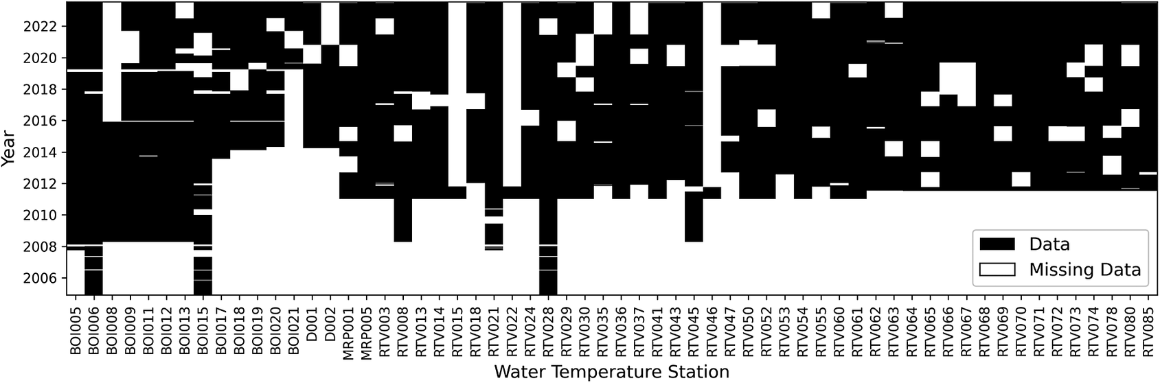
Water temperature data were obtained from a network of water temperature stations maintained across the rivers of Vaud. Figure 1 shows the geographical distribution of such stations. A total of 60 stations were sampled at a resolution of 1 h between 2006 and 2023. Figure 2 shows the availability of data through time. For model development, hourly records were aggregated to daily statistics. We focused primarily on the 90th percentile of daily water temperature, defined as the temperature below which 90% of the hourly observations occur. Compared with the daily maximum, this metric is less sensitive to short-lived spikes or measurement errors. At the same time, it still captures the higher temperature conditions experienced during the day, which are particularly relevant for aquatic organisms because elevated temperatures can induce physiological stress (Elliott and Elliott, Reference Elliott and Elliott2010).
Location of water temperature stations in the Canton of Vaud. The inset (top left) displays the map of Switzerland, with a red rectangle indicating the study area’s geographic extent.

Figure 1. Long description
The figure shows the spatial distribution of the study’s water temperature stations in the Canton of Vaud, western Switzerland. Blue points indicate station locations along streams, with a concentration along the Boiron, Venoge, and Broye rivers and additional stations distributed across other streams. The background layer represents tree height, ranging from 0 to 40 m, illustrating variation in riparian vegetation across the study area. Monitoring sites are located across a gradient of vegetation conditions, including areas with dense tree cover and areas with limited or no riparian vegetation, allowing the study to capture a range of environmental contexts. Two inset maps provide geographic reference: the first shows the position of the Canton of Vaud within Switzerland, marked by a red rectangle, and the second shows Switzerland’s location within Europe and its proximity to neighboring countries, including France, Germany, and Italy.
Data availability for each water temperature station. Black means water temperature measurements are available.
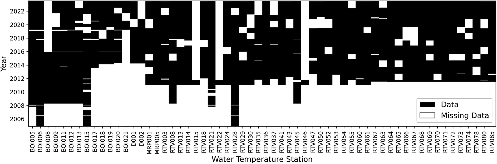
The figure is a binary matrix showing the temporal coverage of water temperature measurements for each water temperature station (60 in total). Stations are listed on the horizontal axis, and years from 2005 to 2023 are shown on the vertical axis. Each cell represents one station–year combination. Black cells indicate years for which water temperature measurements are available, while white cells indicate missing measurements.
The figure illustrates differences in monitoring duration and data completeness among water temperature stations. Some stations have continuous records spanning several years, whereas others show intermittent measurements or longer periods without data. Most stations have limited or no data before 2012. A few stations, including RTV015, RTV022, and RTV046, contain measurements for only a single year.
2.1.2. Meteorological data
Meteorological data were provided by the Federal Office of Meteorology and Climatology (MeteoSwiss, 2025) and include a wide range of atmospheric and surface variables. The main available features can be grouped as temperature/radiation, pressure, evaporation, wind, cloud, and precipitation-based (Table 1). These groups correspond directly to the structure used in the model, where meteorological variables are organized into the same domain-specific categories for grouped processing. Temperature and radiation variables were grouped because they both affect the amount of heat transferred to the stream and are typically highly correlated. This information provides the climate context needed to explain the temporal variability of stream water temperature and allows the model to capture both seasonal cycles and weather-driven fluctuations.
Meteorological features from MeteoSwiss used in this study, including their code and unit

Table 1. Long description
The table summarizes the meteorological features from MeteoSwiss used in the study, including feature names, MeteoSwiss codes, and measurement units. The features are organized into seven groups: Temperature/Radiation, Pressure, Evaporation, Wind, Cloud, Hydrometeorology, and Snow. Temperature/Radiation includes air and soil temperature variables and radiation measurements (global, diffuse, incoming longwave, outgoing longwave, and reflected shortwave radiation). Pressure includes variables reduced to sea level and measured at station altitude. Evaporation includes reference evaporation and evapotranspiration. Wind includes maximum hourly mean and daily mean wind speed. Cloud includes cloud cover, high cloud-cover days, dark days, and fog occurrence. Hydrometeorology includes precipitation, relative humidity, and rainy days. Snow includes snow coverage, fresh snow accumulation over 48 hours, and snowfall occurrence.
2.1.3. Vegetation data
To characterize riparian canopy structure, we used the Vegetation Height Model (VHM; Figure 1) (Ginzler and Hobi, Reference Ginzler and Hobi2015) derived from aerial stereo images of a spatial resolution of 1 m, and to estimate vegetation density and health, we derived the Specific Leaf Area Vegetation Index (SLAVI) (Lymburner et al., Reference Lymburner, Beggs and Jacobson2000) from the Landsat 8 satellite imagery which has a spatial resolution of 30 m. These layers were extracted around each water temperature station and along upstream segments of the river network to capture the potential influence of riparian vegetation on water temperature. VHM and SLAVI were normalized between 0 and 1, and then merged using a product in order to have high values of the resulting index only if both SLAVI and VHM are high. This combination of VHM and SLAVI is used to get images of high spatial resolution through VHM and high temporal resolution through SLAVI.
2.1.4. Other data
In addition to hydrological, meteorological, and vegetation datasets, we included topographic and temporal descriptors. These consist of the altitude of each water temperature station, the day of the year (encoded as sine and cosine of the day as an angle), and the local slope of the river upstream of each station. Consistent with the 20 m segmentation approach used for riparian vegetation extraction, river elevations are extracted along the 500 m reach upstream of the water temperature station. This unitless slope is then defined as the vertical drop between a point located 500 m upstream and the station, divided by the 500 m horizontal distance (multiplied by 100 to obtain a percentage). To calculate the slope, we use the final 480 to 500 m segment. If tributaries join the mainstem within this upper segment, the elevations of all contributing branches are averaged to account for the multiple channels.
These variables were also used by the model. Altitude and day of the year (encoded using sine and cosine transformations) were used as individual predictors, whereas slope plays a dual role: it is used both as an individual predictor and to allow the spatial influence of vegetation to vary as a function of upstream slope. Further details on how these features are used by the model are provided in Section 3.1.2.
2.2. Feature engineering
2.2.1. Pre-processing
To remove erroneous data, we removed observations with water temperatures lower than 0 °C and higher than 30 °CFootnote 1. Before training, input features were standardized to have a mean of zero and a standard deviation of one using the StandardScaler implementation from the Python library scikit-learn (Pedregosa et al., Reference Pedregosa, Varoquaux, Gramfort, Michel, Thirion, Grisel, Blondel, Müller, Nothman, Louppe, Prettenhofer, Weiss, Dubourg, Vanderplas, Passos, Cournapeau, Brucher, Perrot and Duchesnay2018). Similarly, vegetation features (SLAVI–VHM raster images) were also standardized to have a mean of zero and a standard deviation of one at the raster level.
2.2.2. Interpolation of meteorological features
Meteorological variables from MeteoSwiss were interpolated to the locations of the water temperature stations using inverse distance weighting (IDW) (Shepard, Reference Shepard1968). For each day and variable, observations from surrounding meteorological stations were weighted by the inverse squared horizontal distance to each water temperature station, giving greater influence to nearby meteorological stations. This procedure provides daily estimates of each meteorological variable at every river temperature monitoring location. For air temperature, differences in elevation between meteorological stations and water temperature stations were explicitly accounted for. Air temperature measurements were first adjusted to sea level using a fixed environmental lapse rate of −5.5 °C per 1000 m of elevation change. These sea-level-adjusted values were then interpolated to each water temperature station using IDW, and finally projected back to the altitude of the respective water temperature station.
2.2.3. Extracting upstream stream graph
To quantify riparian vegetation upstream of the water temperature stations, hydrological flow directions were determined, and a network graph was constructed to facilitate the extraction of upstream geolocations at specific intervals (see Section 2.2.4). As the stream shapefiles lacked directional metadata, flow direction was derived from the DHM25 digital height model (SwissTopo, 2025). Subsequently, a directed graph was created using the NetworkX Python library (Hagberg et al., Reference Hagberg, Schult, Swart, Varoquaux, Vaught and Millman2008) to facilitate traversing the stream network and extracting upstream coordinates at defined distances.
2.2.4. Feature extraction from upstream vegetation
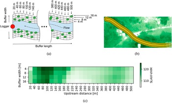
Upstream vegetation was characterized using 1 m resolution raster data (i.e., SLAVI-VHM) along river networks upstream of each water temperature station. The upstream network was divided into segments of 20 m up to a maximum distance of 500 m, and each segment was buffered at multiple widths: 4, 8, 12, and 16 m, to capture vegetation effects at different spatial scales. Vegetation features were extracted by computing the mean of pixel values within each buffer for every segment, averaging the left and right banks together. For rasters with multiple years, mean values were computed for each year separately. Figure 3a illustrates the method used to extract data from the raster, while Figure 3b shows an example of the different buffer widths and lengths upstream of a water temperature station, overlaid on a SLAVI-VHM raster.
(a) Buffer zones (characterized by length and width, with left and right banks averaged together) used to compute vegetation features along the river. (b) Example on an actual satellite image showing the different buffer zones for a given segment of the river. (c) Example of upstream vegetation for one water temperature station (data from year 2013). The darker the green color, the higher the SLAVI-VHM.

Figure 3. Long description
Panel a is a schematic diagram of a river buffer. At the center is a blue river with a dashed arrow indicating Flow. A red circle labeled Logger is at the downstream end. The buffer length is divided into segments from 20 m to 500 m. The buffer width is divided into four parallel zones on each side of the river, labeled 4 m, 8 m, 12 m, and 16 m. Green tree symbols are scattered within these zones.
Panel b is an aerial photograph showing a green forested landscape. A yellow, multi-layered curved path representing the buffer zones follows the course of a river through the center of the terrain.
Panel c is a heat map. The x-axis is Upstream distance in meters, ranging from 20 to 500 in increments of 20. The y-axis is Buffer width in meters, with rows for 4, 8, 12, and 16. A color scale on the right indicates S L A V I - V H M values from 110 in light green to 120 in dark green. The highest values, indicated by the darkest green, are concentrated between 60 m and 120 m upstream distance across all buffer widths.
The figure group illustrates the method used to characterize river vegetation using buffer zones. Panel (a) shows a schematic of river buffer zones defined by different buffer lengths and widths along the upstream direction of a river segment. The left and right river banks are averaged together, and vegetation features are calculated within each buffer zone. Panel (b) shows an example satellite image of a river section with multiple buffer zones overlaid along the channel. Panel (c) presents a heatmap showing vegetation index values (SLAVI-VHM) along the upstream distance of a river segment for different buffer widths. Darker green areas indicate higher vegetation index values.
A schematic river segment is shown with the flow direction indicated from left to right. A logger location is marked on the left side. Rectangular buffer zones extend upstream along the river, with example buffer lengths labelled from 20 m to 500 m and buffer widths labelled from 4 m to 16 m. Vegetation symbols are distributed along both river banks. The diagram indicates that vegetation characteristics are averaged from the left and right banks within each buffer zone.
A satellite image shows a river channel surrounded by green vegetation, with several parallel yellow outlines following the stream to represent different buffer zones and upstream distances used to extract average vegetation values along the river segment.
A rectangular heatmap displays SLAVI-VHM vegetation index values calculated for different upstream distances and buffer widths. The horizontal axis represents upstream distance from 20 m to 500 m, and the vertical axis represents buffer width from 4 m to 16 m. Green color intensity represents vegetation index values, with darker green indicating higher values. The highest values occur near the beginning of the river segment, around 60–120 m upstream, while lower values occur through much of the middle section before increasing slightly near the downstream end. The resulting matrix of average vegetation values for each combination of upstream distance and buffer width can be used as input data for a model.
Upstream vegetation can consequently be represented as an image with the distance along the river on one axis and the width perpendicular to the river on the other axis. Figure 3c shows an example of such an image.
3. Methods
This section describes the machine learning model, its architecture, and the training methodology used in this study.
3.1. Model architecture
We trained an artificial neural network based on a Multi-Layer Perceptron (MLP) architecture, which processes input data through successive layers of interconnected neurons. The model includes custom layers designed to enhance interpretability. Section 3.1.1 describes these custom layers.
3.1.1. Grouped inputs and attention component
The input features were organized into domain-specific groups. Meteorological features were grouped as shown in Table 1: temperature, wind, pressure, hydrometeorological, cloud cover, evaporation, and snow. Vegetation-related features were also grouped. Temporal variables (sine and cosine of the day of the year) and topographic features (altitude and slope) were included as individual predictors. This grouping strategy reflects the distinct physical drivers of river thermal dynamics and allows the model to process each category using a dedicated computational module. Moreover, grouping features reduces the number of free parameters in the model, thereby limiting complexity and the risk of overfitting, while improving interpretability of feature contributions.
For meteorological data, a weighting scheme was implemented to capture the relative contribution of individual predictor within each group described in Table 1. Within each group, feature weights were normalized using the Softmax function (Bridle, Reference Bridle, Soulié and Hérault1990), which transforms the raw values into positive weights that sum to one. These normalized weights are then used to compute a weighted average of the features, resulting in a single summary value for the entire group. This allows the model to represent the relative importance of each feature within the group, where higher weights indicate features that are more strongly considered by the model when forming the group summary. The weights are found during the training of the model, as described in Section 3.2. This Softmax-based weighting provides a compact and interpretable representation of each meteorological group. Figure 4 describes this custom Softmax weighting strategy for one individual group.
Schematic representation of the softmax-based weighting used to summarize meteorological feature groups. This scheme represents one group. Each group is handled as an independent unit. Features within a group range from
$ {X}_1 $
 to
$ {X}_n $
 .

Figure 4. Long description
The diagram illustrates the softmax-based weighting process used to summarize one meteorological feature group. The group contains multiple features, labelled Group Feature X subscript 1 through Group Feature X subscript n. Each feature is assigned an attention weight w subscript i. The weighted features are passed to a SoftmaxAttention1D layer, which applies the softmax operation to the weight matrix W multiplied by the input feature matrix X. The resulting weighted values are combined using an average layer to produce a summarized representation of the feature group.
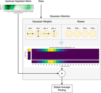
As far as vegetation data is concerned (see Section 2.2.4), we designed and implemented a Gaussian attention module. The upstream vegetation images have mean values of riparian vegetation at different buffer widths and distances around rivers. Logically, all riparian vegetation locations do not have the same impact on water temperatures. For instance, a narrow river would not get the same temperature reduction from a tree that is 16 m away from the river’s center than from a tree 4 m away. This calls for a way to put more weight on certain locations than others. Another thing to consider is that there is a high correlation between neighboring riparian vegetation locations. This leads to the inclusion of an attention module that can leverage the spatial structure of these vegetation matrices. This approach is referred to as “Gaussian attention” in this paper. As you can see on Figure 5, the upstream vegetation is fed to the Gaussian attention layer as a matrix. To allow the model to focus on the most relevant locations, the upstream vegetation matrix is multiplied by a matrix of weights that sum to 1. In this manner, the model is enabled to consider only the most informative pixels and to ignore values that are not useful for prediction. A two-dimensional Gaussian function is used to construct this weight matrix. The use of a Gaussian function to weight pixels is motivated by the spatial structure of the vegetation images and by the assumption that there exists a location where the impact on the sensor’s water temperature is the highest, and that the further this location is from that point, the smaller the impact becomes. This allows the conservation of as many locations as desired without increasing the number of parameters. Indeed, instead of learning weights for each location (100 weights in this case), only the shift and spread of this two-dimensional Gaussian function are learnedFootnote 2.
Architecture of the upstream vegetation Gaussian attention layer. The layer takes two inputs: the upstream vegetation represented as a matrix, and the water temperature station slope, which determines the shape and position of the Gaussian. The model learns eight parameters, including the Gaussian standard deviations (defining width and height), the positions along both horizontal and vertical axes, and the biases. The resulting attention matrix is subsequently multiplied with the upstream vegetation matrix, effectively assigning greater weight to the most relevant riparian vegetation zones. In this specific example, the attention matrix, dependent on the station slope, assigns higher weights to vegetation located approximately 140 to 160 meters upstream of the water temperature station, with a width of 4 m (highlighted in yellow in the figure). Finally, a Global Average Pooling layer produces a single summary value representing the riparian vegetation.

Crucially, in our implementation, the parameters of the Gaussian function are modulated by the feature slope, providing context that guides the model’s attention. Figure 5 illustrates how the attention depends on the slope. This allows the model to dynamically assign more importance to vegetation locations depending on local topography. In this manner, the model can adapt its spatial focus to riparian vegetation in a way that is both context-aware and easily interpretable and visualizable after training.
Together, the Softmax and Gaussian attention module provide a flexible attention framework that enhances predictive accuracy while yielding interpretable weights linked to ecological processes.
3.1.2. Stream water temperature regression head
The first component of our model (see Section 3.1.1) summarizes each group of input features into a single, interpretable group summary. These summaries are computed as weighted averages of the features, where the weights are determined by the attention module to reflect the relative importance of each variable. In addition to these grouped summaries, four individual features (slope, altitude, and the sine and cosine encoding of the day of the year) are not included in any group and are directly concatenated with the group summaries. The slope variable therefore has a dual function in the architecture: it modulates the Gaussian attention module for vegetation features and is also included as a direct predictor in the regression head.
The resulting vector, composed of all group summaries and the four ungrouped features, is passed through an MLP, which is a type of artificial neural network that processes input data through multiple layers of interconnected artificial neurons. Each layer performs a series of linear and nonlinear transformations, allowing the model to capture complex relationships among features. In our MLP, the concatenated feature vector is processed by two hidden layers of neurons. Finally, a single output neuron predicts the daily 90th percentile stream water temperature.
The overall model architecture is summarized in Figure 6.
Overall architecture of the model. Each group of features is summarized by a single value representing a weighted average of all features within the group. A more complete description of meteorological individual features can be found on Table 1. For meteorological groups, feature weights are constrained by the Softmax function, which transforms raw scores into positive weights that sum to one, ensuring an interpretable relative contribution of each variable. For vegetation features, a Gaussian attention module assigns spatially structured weights based on a two-dimensional Gaussian function whose parameters are modulated by slope, enabling context-aware spatial focus on the most relevant riparian zones. Four additional features (slope, altitude, and the sine and cosine encoding of the day of the year) are not grouped and are directly concatenated with the group summaries. The slope variable therefore plays a dual role: it modulates the Gaussian attention mechanism and is also provided as a direct input to the concatenated feature vector. The resulting vector is passed to an MLP composed of two hidden layers, which performs nonlinear transformations to predict the daily 90th percentile stream water temperature. The weights are learned by the model during model training, as described in Section 3.2.

3.2. Model training
3.2.1. Evaluation policy
Model performance was evaluated using a spatial cross-validation strategy with spatial-kfold (Ghariani, Reference Ghariani2023), using 500 m blocks. The data were split into
$ k=10 $
 folds so that water temperature loggers in the training set were not located close to those in the held-out fold. After training, predictions were generated on the held-out fold, and the mean absolute error (MAE) was computed to assess model accuracy. This cross-validation was used purely for performance evaluation, not for hyperparameter selection.
3.2.2. Evaluation metrics
Model performance was evaluated using MAE, which measures the average magnitude of the prediction error without considering its direction. MAE is defined as:

where
$ {T}_{w,i}^{pred} $
 and
$ {T}_{w,i}^{obs} $
 denote the predicted and observed water temperatures for observation
$ i $
 , and
$ N $
 is the total number of observations. MAE provides an easily interpretable measure of prediction error expressed in the same units as the target variable (°C).
3.2.3. Hyperparameters
The model was trained for 50 epochs, which was sufficient for convergence, with a batch size of 32 (the default in Keras). The Adam optimizer (Kingma and Ba, Reference Kingma and Ba2017) was used with a learning rate of 0.0001, reduced from the default of 0.001 to improve training stability. A Dropout of 0.1 was introduced between the two dense hidden layers of our MLP to reduce overfitting by randomly deactivating 10% of neurons during training, which helps the model to generalize to unseen data.
The loss function was log-cosh (Saleh and Saleh, Reference Saleh and Saleh2024), which is robust to outliers while penalizing deviations smoothly, making it suitable for environmental time series with occasional extreme values. No extensive hyperparameter tuning was performed; the values were chosen based on convergence behavior and standard defaults in the Keras implementation.
4. Results
This section presents the performance of the model described in Section 3 and analyzes the learned attention mechanisms and vegetation effects on stream water temperature.
4.1. Model performance
The proposed modeling framework yields a median MAE of 1.31 °C across the
$ 10 $
 spatial cross-validation folds (see Figure 7). The use of spatial cross-validation ensures that geographically close water temperature stations, likely to share similar hydrological and thermal characteristics, are not included in the same fold. This approach reduces the risk of overfitting and provides a more conservative yet realistic estimate of model generalization to unseen locations.
Boxplot of the Mean Absolute Error (MAE) across the 10 spatial cross-validation folds. The model attained a median MAE of 1.31 °C. For comparison, a recent review of machine learning studies on stream water temperature reported testing MAE values with an interquartile range of 0.55–1.53 °C and a median of 1.21 °C across 13 studies (Corona and Hogue, Reference Corona and Hogue2025).

Figure7. Long description
The boxplot shows the validation mean absolute error in degrees Celsius. The errors range from approximately 1 degrees Celsius to 1.9 degrees Celsius. The individual validation folds are shown as blue dots at values of approximately 1, 1.1, 1.22, 1.25, 1.26, 1.37, 1.64, 1.65, 1.76, and 1.9 degrees Celsius. The median error is 1.31 degrees Celsius. The central half of the errors falls between approximately 1.22 and 1.65 degrees Celsius.
Although spatial partitioning tends to yield slightly lower performance compared to random cross-validation, the resulting MAE on testing procedures remains within the range reported in recent machine learning studies of stream water temperature. For example, a review by Corona and Hogue, Reference Corona and Hogue2025 reported MAE values on testing datasets with an interquartile range of 0.55–1.53 °C and a median value of 1.21 °C across 13 studies. Our results therefore fall within the range of previously published work, demonstrating the robustness and relevance of the proposed modeling framework.
4.2. Interpretation of vegetation attention
A great advantage of the particular neural network architecture used is that, although being a black-box model, it allows the interpretation of the parameters found by the training algorithm. For example, we can visualize how the model focuses on riparian vegetation information from each upstream segment to effectively predict stream water temperature. Figure 8, shows the resulting upstream Gaussian vegetation attention as a function of the slope for our final model. The more yellowish the color, the higher the focus.
Visualization of the riparian vegetation segment’s attention on all data as a function of the slope. The more yellowish the color, the higher the focus of the model on that particular upstream segment.

The figure contains two heatmaps showing the model’s attention to riparian vegetation along river segments. Both heatmaps show attention values as a function of slope, with slope values ranging from 0.2% to 1.1%.
The left heatmap shows attention across buffer widths in meters from the river channel. The model consistently focuses on a buffer width of 4 m, corresponding to the area closest to the river channel, for all slope values.
The right heatmap shows attention across upstream distances in meters as a function of slope. The preferred upstream distance varies with slope. At a slope of 0.2%, the model focuses on distances between approximately 40 and 220 meters, with peak attention around 120 meters. At a slope of 1.1%, attention shifts further upstream, between approximately 220 and 440 meters, with peak attention around 340 meters. This shows that the model considers longer upstream distances as slope increases.
Thus, we can observe that when the slope is low, models tend to focus more on the vegetation close to the water temperature stations. In contrast, when the slope is high, attention shifts towards upstream vegetation located further away. This result is consistent with the idea that steeper slopes lead to faster water flow (assuming other factors remain constant), emphasizing the influence of upstream vegetation on stream water temperature. These results suggest that accurately predicting water temperature requires considering not just the target location but also the upstream environment through which the water has flowed.
4.3. Impact of vegetation on water temperatures
To quantify the influence of riparian vegetation on predicted water temperature, we performed a sensitivity analysis on the neural network trained with all the data. Specifically, we varied the activation of the neuron summarizing the SLAVI–VHM vegetation features. The resulting model response is shown in Figure 9.
Mean model response of predicted water temperature (
$ {T}_w $
 ) to variations in the vegetation feature SLAVI-VHM, showing cooler temperatures with increasing vegetation density. The upper 10% of the warmest days were used.

Figure 9. Long description
The figure has an x axis with the riparian vegetation and a y axis with the Predicted Water Temperature. The temperatures range from 15 to 22 and the riparian vegetation values are the activation values inside the model, ranging from −0.016 to 0.012. The temperatures represent the upper 10% temperatures of the warmest days. The line starts at slightly more than 19° and decreases gradually to approximately 16.6 degrees Celsius as the riparian vegetation values increase. The standard deviation is also shown. It starts wider, ranging between 16.5° and 22°, and finishes narrower, ranging from slightly more than 15 up to approximately 18.
Thus, the activation of the vegetation node within the model spans values from approximately
$ -0.016 $
 (corresponding to the absence of forest cover) to 0.012 (dense riparian forest conditions). The analysis focuses on the upper 10% of the warmest days (90th percentile), during which vegetation is expected to exert its strongest thermal regulation effect. Counterfactual simulations were conducted by systematically increasing the SLAVI–VHM activation across all selected data points, while maintaining all other inputs constant. The results reveal a clear inverse relationship between riparian forest and the predicted water temperature (
$ {T}_w $
 ): as vegetation density increases, model outputs indicate a consistent cooling effect. The difference between the lowest and highest observed activations of the SLAVI–VHM group corresponds to an average reduction of nearly 3 °C in the predicted water temperature.
To complement this analysis, we applied SHAP (SHapley Additive exPlanations) (Lundberg and Lee, Reference Lundberg and Lee2017) to quantify the contribution of each feature to the model’s output. Figure 10 shows the resulting SHAP beeswarm visual summary of feature importance and the direction of their effects. Each point represents one observation, with color indicating feature value. As expected, temperature-related features emerge as the most influential ones. Importantly, riparian vegetation is among the top contributors, with higher vegetation values consistently associated with lower predicted water temperatures, reflecting its cooling effect. The model also captures the significant impact of altitude on the water temperature. Evaporation-related features are influential, but in the opposite direction: higher values are linked to increased predicted water temperature. Overall, both sensitivity and SHAP analyses consistently indicate that riparian vegetation has a strong cooling effect on stream water temperature, supporting the physical plausibility of the model and highlighting the ecological relevance of riparian shading and microclimate effects.
SHAP analysis of feature impacts on predicted water temperatures. Color indicates feature value (bluer = lower, pinker = higher), and horizontal position shows contribution to the prediction. SLAVI-VHM is the upstream riparian vegetation group. The seven other features mentioned in the figure are: slope, ordinal day (sin encoded), hydrometeorology, cloud, snow, pressure, and wind.

Figure 10. Long description
This horizontal beeswarm plot shows a SHAP analysis of feature impacts on predicted water temperatures. Six feature groups are ranked top to bottom by importance: Group temperature, day cos, altitude, Group evaporation, SLAVI-VHM (upstream riparian vegetation), and the sum of 7 other features (slope, ordinal day sin-encoded, hydrometeorology, cloud, snow, pressure, wind). Each dot is one data point; horizontal position shows its SHAP value, and color shows the feature’s actual value, from blue (low) to red (high). Group temperature dominates, with high values driving strong positive contributions. Notably, SLAVI-VHM shows a clear inverse pattern: low vegetation values (blue) push predictions higher, while high vegetation values (red) push predictions lower, highlighting riparian vegetation’s cooling effect on water temperature, an ecologically meaningful result.
5. Conclusion
Our results demonstrate that riparian vegetation significantly modulates water temperature, with effects that are both physically plausible and consistent with known hydro-ecological processes. The model identified that when local reach slope was low, the influence of upstream riparian vegetation extended only a short distance upstream, whereas in steeper reaches, upstream riparian vegetation exerted influence over longer upstream distances. This pattern is consistent with hydrological reasoning: in steeper reaches, faster flow reduces water residence time, making upstream vegetation more influential in shaping downstream temperatures. Conversely, in flatter terrain, slower-moving water allows local riparian shading and microclimatic effects to dominate, consistent with previous descriptions of the physical controls governing stream thermal regimes (Caissie, Reference Caissie2006; Carrivick et al. Reference Carrivick, Brown, Hannah and Turner2012).
Given the stochastic nature of the training procedure to obtain data-driven models, and to the small number of observations available, we obtained varying results regarding the importance of riparian buffer width across different model configurations. In earlier versions, the model tended to focus on wider buffer zones under low-slope conditions, likely because rivers are broader in flatter terrain and narrower buffers may overlap the river channel itself, failing to fully capture riparian vegetation. In contrast, in our final model, we observe that a relatively narrow riparian buffer is sufficient to provide a measurable cooling effect, consistent with local shading and near-bank microclimate modulation being the primary mechanisms. Wider zones contribute little additional cooling, suggesting that lateral or more distant vegetation effects might be secondary at the spatial scales considered. While riparian zones are widely recognized as complex interfaces between terrestrial and aquatic ecosystems whose ecological influence can extend beyond narrow streamside areas (Gregory et al., Reference Gregory, Swanson, McKee and Cummins1991), our results indicate that, for the specific aspects of thermal regulation captured by the model, the most influential processes operate at relatively short distances from the channel. This finding is consistent with previous work identifying riparian shading as one of the dominant controls on stream thermal regimes (Dan Moore et al., Reference Dan Moore, Spittlehouse and Story2005; Garner et al., Reference Garner, Malcolm, Sadler and Hannah2017), while further suggesting that, within our study area, vegetation closest to the channel contributes most strongly to the cooling signal captured by the model. This interpretation should be viewed in light of the inherent simplification of data-driven models, which only include a subset of riparian and catchment variables and therefore cannot explicitly represent other processes such as nutrient dynamics or broader microclimatic interactions. Our results are nevertheless consistent with previous studies showing that shaded reaches can be several degrees cooler than exposed reaches (Kalny et al., Reference Kalny, Laaha, Melcher, Trimmel, Rauch and Schmutz2017; Dugdale et al., Reference Dugdale, Malcolm, Kantola and Hannah2018), and that even relatively narrow riparian strips can provide meaningful thermal regulation as long as the stream is fully shaded throughout the day (Fuller et al., Reference Fuller, Leinenbach, Detenbeck, Labiosa and Isaak2022). The physical plausibility of the model’s attention patterns and sensitivity analyses, particularly the inverse relationship between vegetation density and predicted water temperature, indicates that the model’s behavior is consistent with well-established physical drivers of stream temperature.
By combining spatially explicit vegetation metrics with topographic and meteorological predictors, our study complements recent efforts to integrate remote sensing and machine learning for stream temperature prediction (Zhu and Piotrowski, Reference Zhu and Piotrowski2020), while highlighting the nuanced interplay between slope, upstream contributions, and near-channel vegetation in shaping river thermal regimes. These findings further support the recognition that riparian vegetation plays a central role in mitigating stream warming and maintaining suitable thermal conditions for aquatic ecosystems (Turunen et al., Reference Turunen, Elbrecht, Steinke and Aroviita2021). This provides actionable insight for river management, indicating that targeted planting or preservation of riparian vegetation, even within narrow corridors, could yield measurable thermal benefits for aquatic ecosystems. These findings are also consistent with previous restoration studies demonstrating that strategically increasing riparian shading can reduce stream temperatures (SJ Dugdale et al., Reference Dugdale, Malcolm and Hannah2024). Importantly, our model can also be used to suggest locations where riparian planting would be most effective to reduce water temperatures at specific sites, enabling data-driven decisions for restoration or conservation planning aimed at preserving or enhancing stream thermal refugia (Sullivan et al., Reference Sullivan, Vokoun, Helton, Briggs and Kurylyk2021).
As a limitation, our model does not account for discharge, as insufficient discharge data were available. In addition, meteorological variables are derived through spatial interpolation from nearby stations, which introduces uncertainty and provides only a rough approximation of true local conditions. Our analysis is also limited to the Canton of Vaud; extending it to other regions would help assess the robustness of the findings across a broader range of hydro-climatic settings.
Regarding vegetation importance, our Gaussian attention-like module assumes a symmetric influence of riparian vegetation around a central focal point, as the weighting is derived from a two-dimensional Gaussian function. However, in practice, the spatial influence of vegetation is unlikely to be perfectly symmetric, as certain portions of the riparian corridor, such as those located closer to the water temperature station, may exert a stronger effect.
These methodological assumptions, together with regional and data limitations, might have contributed to slight variations in the estimated riparian importance across experiments, as well as in model performance (MAEs). Nevertheless, performances were quite robust and generally remained within ranges similar to other state-of-the-art studies (Corona and Hogue, Reference Corona and Hogue2025). Furthermore, the general trend, showing strong cooling effects of vegetation and a consistent shift of attention with slope, remained stable and supports the robustness of the main findings.
In future studies, the predictive accuracy and applicability of our framework could be enhanced by addressing the current limitations listed above. Future work could also explore climate change scenarios to evaluate how riparian vegetation might buffer stream water temperature increases under different warming trajectories. It would also be interesting to extend the context given to the Gaussian attention module used for summarizing SLAVI-VHM, i.e., to include other relevant characteristics besides slope. This would provide a more complete understanding of how those characteristics impact the relationship between vegetation and stream water temperature. And thus, providing better tools for supporting reforestation strategies. Additionally, generating spatially explicit maps would help identify locations where reforestation or targeted riparian planting would have the greatest overall impact on cooling stream water, supporting effective, data-driven management and restoration strategies.
Data availability statement
The code used in this study is publicly available at https://github.com/SimWalther/ML4Water/. River temperature data are partially available from the General Directorate of the Environment of the Canton of Vaud (www.vhv-qualite.ch) upon request, and partially owned by La Maison de la Rivière (https://www.maisondelariviere.ch/). Meteorological data were provided by the Federal Office of Meteorology and Climatology (MeteoSwiss, 2025). The Vegetation Height Model (VHM) was obtained upon request from the authors of the “Vegetation Height Model NFI” (Ginzler and Hobi, Reference Ginzler and Hobi2015). SLAVI data are publicly available and were accessed via Google Earth Engine. Altitude data are from the DHM25 model, available at https://www.swisstopo.admin.ch/.
Acknowledgments
We are grateful to the team from “La maison de la rivière” who provided the data from temperature loggers, and actively participated in fruitful discussions that shaped the contribution.
Author contribution
Conceptualization: All. Data curation: S.W, B.H, H-F.S. Formal Analysis: All. Funding Acquisition: A.P., J.-F.R. Investigation: All. Methodology: All. Project Administration: A.P., J-F.R. Data Collection: P.L., J-F.R., S.W., B.H., H.-F.S. Software: S.W., B.H., H.-F.S. Supervision: A.P., J.-F.R. Visualization: S.W., B.H., H.-F.S. Writing original draft: S.W., B.H., H.-F.S. Writing—review & editing: All.
Funding statement
This research was supported by the grant IA-RECHERCHE23–18 of the I&A Engineering and Architecture domain of the HES-SO University of Applied Sciences and Arts Western Switzerland.
Competing interest
None.
Ethics statement
The research meets all ethical guidelines, including adherence to the legal requirements of the study country.
Generative AI usage declaration
During the preparation of this manuscript, the authors used generative artificial intelligence (GAI) tools, including ChatGPT (OpenAI, GPT-5), and Le Chat (Mistral), to assist with language editing, improving clarity of expression, and providing suggestions for restructuring paragraphs to enhance logical flow. These tools were employed solely to improve the linguistic quality of the text, including grammar, style, readability, and organization. All scientific ideas, analyses, interpretations, and conclusions presented in this work are entirely the authors’ own. After using these tools, the authors carefully reviewed, verified, and edited all content, and take full responsibility for the scientific integrity and accuracy of the published work.








 Open access

