Introduction
Camera trapping is a well-established and popular method for monitoring biodiversity, and using remotely triggered cameras (camera traps) is a relatively low-cost and widely used approach. In many situations, it is not feasible to mark or individually distinguish animals, and camera trap data are used to generate occupancy data and indices of relative abundance of multiple species simultaneously (Royle et al. Reference Royle, Chandler, Sollmann and Gardner2014; Parsons et al. Reference Parsons, Forrester, McShea, Baker-Whatton, Millspaugh and Kays2017). Indices of relative abundance are commonly assumed to have a direct, linear, and constant relationship with wildlife density (Pollock et al. Reference Pollock, Nichols, Simons, Farnsworth, Bailey and Sauer2002); however, this assumption is rarely realistic (Sollmann et al. Reference Sollmann, Mohamed, Samejima and Wilting2013; Parsons et al. Reference Parsons, Forrester, McShea, Baker-Whatton, Millspaugh and Kays2017). Despite good correlation between detection rates and density for many ungulate species, a large body of literature shows that factors other than density affect the number of animals photographed or captured on camera traps, and the consensus is that methods to estimate abundance accounting for imperfect detection is preferred to methods that rely on indices (Kays et al. Reference Kays, Arbogast, Baker-Whatton, Beirne, Boone, Bowler, Burneo, Cove, Ding, Espinosa, Concalves, Hansen, Jansen, Kolowski, Knowles, Lima, Millspaugh, McShea, Pacifici, Parsons, Pease, Rovero, Santos, Schuttler, Sheil, Si, Snider and Spironello2020).
Obtaining accurate population estimates is one of the most elementary needs for wildlife management, particularly introduced ungulates on oceanic islands. On Guam (known as Guåhan in the Chamorro language), Philippine deer (Rusa marianna; Wiles Reference Wiles2012) and wild pigs (Sus scrofa; Hess et al. Reference Hess, Wehr, Litton, Vercauteren, Beasley, Ditchkoff, Mayer, Roloff and Strickland2020; wild boar and descendants of domestic pigs) cause agricultural and ecological damage and are hunted for recreational, nutritional, and cultural uses. In areas of high conservation value, land managers are required to eradicate ungulates (e.g., JRMNRS 2012). In these areas, understanding population size and the efficacy of control efforts is important for effective conservation management. In other areas of the island, land managers are tasked with the management of both ungulates as game species and understanding population size is needed for maintaining a sustainable harvest. Based on the decision tree by Gilbert et al. (Reference Gilbert, Clare, Stenglein and Zuckerberg2021), distance sampling with camera traps is the most appropriate method for estimating densities of unmarked deer and pig populations on Guam and tropical islands. Camera trap distance sampling (CTDS) allows for non-independent observations of multiple detections of an unmarked animal and imperfect detection where some individuals present are not detected (Howe et al. Reference Howe, Buckland, Despres-Einspenner and Kühl2017). Distance sampling has a well-described theoretical framework to account for imperfect detection and is a core wildlife monitoring method for estimating densities of unmarked populations (Buckland et al. Reference Buckland, Anderson, Burnham, Laake, Borchers and Thomas2001, Reference Buckland, Anderson, Burnham, Laake, Borchers and Thomas2004, Reference Buckland, Rextad, Marques and Oedekoven2015; Thomas et al. Reference Thomas, Buckland, Rexstad, Laake, Strindberg, Hedley, Bishop, Marques and Burnham2010). In general, distance sampling involves surveying transects or points, measuring the perpendicular or radial distance to detected animals, and fitting a detection function to the distances to estimate densities using a Horvitz-Thompson-like estimator. Point-transect distance sampling is a common form of distance sampling (Buckland et al. Reference Buckland, Rextad, Marques and Oedekoven2015), where at predetermined points, the horizontal radial distance to detected animals is measured. Howe et al. (Reference Howe, Buckland, Despres-Einspenner and Kühl2017) extended the point-transect distance sampling model to accommodate camera trap data and formulated the CTDS method. The adaptation is based on treating camera traps as the observer, instead of humans. For CTDS, stationary cameras detect animals as they move through the camera’s field of view (FOV; Howe et al. Reference Howe, Buckland, Despres-Einspenner and Kühl2017). Thus, additional information beyond the number of animals detected and a calibrated measurement of the distance to each detection animal is needed: a measurement of each camera’s FOV and the temporal sampling effort summed across all cameras (Hofmeester et al. Reference Hofmeester, Rowcliffe and Jansen2017; Howe et al. Reference Howe, Buckland, Despres-Einspenner and Kühl2017).
CTDS has been used to estimate populations of Maxwell’s duiker (Philantomba maxwellii; Howe et al. Reference Howe, Buckland, Despres-Einspenner and Kühl2017), western chimpanzee (Pan troglodytes verus; Cappelle et al. Reference Cappelle, Després-Einspenner, Howe, Boesch and Kühl2019), bighorn sheep (Ovis canadensis; Harris et al. Reference Harris, Butler, Stewart, Rominger and Ruhl2020), Alpine marmot (Marmota marmota; Corlatti et al. Reference Corlatti, Sivieri, Sudolska, Giacomelli and Pedrotti2020), a community of rainforest species (Bessone et al. Reference Bessone, Kühl, Hohmann, Herbinger, N’Goran, Asanzi, Da Costa, Dérozier, Fotsing, Beka, Iyomi, Iyatshi, Kafando, Kambere, Moundzoho, Wanzalire and Fruth2020; Cappelle et al. Reference Cappelle, Howe, Boesch and Kühl2021), and group-living and solitary mountain ungulates (Pal et al. Reference Pal, Bhattacharya, Qureshi, Buckland and Sathykumar2021). Cappelle et al. (Reference Cappelle, Després-Einspenner, Howe, Boesch and Kühl2019) and Harris et al. (Reference Harris, Butler, Stewart, Rominger and Ruhl2020) both compared CTDS estimates against populations of known size and found estimates were consistent with true abundances, while estimates from other studies were less consistent.
Our objectives are three-fold; first to assess if accurate and precise density estimates of deer and wild pigs can be achieved using CTDS methods in a tropical, oceanic island ecosystem. We compared our CTDS estimates with published literature to assess estimator bias. Based on our density estimates, our second objective is to estimate total effort required to achieve a target coefficient of variation. Optimizing sampling effort ensures high estimator precision (i.e., small standard errors) while maximizing sampling efficiencies, and is a broadly applied approach in distance sampling for estimating what precision is required to meet the survey objectives (Buckland et al. Reference Buckland, Rextad, Marques and Oedekoven2015). Our final objective is to apply the lessons we learned while conducting this study to provide best practices for future application of CTDS methods.
Materials and methods
Study area
Guam is in the west-central Pacific (13⁰ 28′ N, 145⁰ 00′ E) and is the southernmost island of the Mariana archipelago. The island is around 45 km long, ranges between 6 and 13 km wide, and encompasses about 541 km2. Major vegetation includes native limestone forest, secondary forest, and savanna (Amidon et al. Reference Amidon, Metevier and Miller2017). Temperatures are warm ranging annually from 22C to 33C, and wet with average annual rainfall of > 2,000 mm, which predominantly falls during the wet season from July to November (Lander & Guard Reference Lander and Guard2003). The study was conducted on the Naval Facilities Engineering System Command Marianas, Andersen Air Force Base (AAFB), at the north end of Guam. We deployed camera traps in two areas of AAFB, an area on the plateau (hereafter Plateau stratum) and on the narrow, coastal terrace (hereafter Tarague stratum) (Figure 1). The Plateau stratum is a Vitex forest with Vitex parviflora as the dominant canopy species (S Vogt, pers. obs.). The Tarague stratum is coconut forest, native forest and a mix of the two forest types. Dominate canopy trees are Cocos nucifera, Ochrosia oppisitofolia, Pisonia grandis and Ficus prolixa (S Vogt, pers. obs.). Densities of deer were expected to be similar between the strata and among forest types, whereas densities of pigs were expected to be higher in the Tarague stratum, particularly in coconut forests. The Plateau stratum consisted of hunting and non-hunting units totalling an area of 985 ha. The Tarague stratum included non-hunting areas totalling 410 ha.
Study area, strata, and layout of camera traps in Andersen Air Force Base, Guam. Black dots are points on a 500 × 500 m regular grid, yellow circles are camera trap points in the Tarague stratum (green polygon), and red circles are camera trap points in the Plateau stratum (pink polygon).

Target species
The Philippine deer, a medium-sized deer native to the Philippines, was intentionally released on Guam probably in 1771 for the purposes of providing food and recreational hunting (Wiles et al. Reference Wiles, Buden and Worthington1999). Deer are prolific, breeding year-round on Guam and producing one fawn per birth. Although the population varies across the island, Wiles et al. (Reference Wiles, Buden and Worthington1999) noted that densities of > 60 deer/km2 have been recorded. The wild pig is native to Europe, Asia, and North Africa, and was introduced to Guam in the late 1600s as a food source (Conry Reference Conry1988). Similar to deer, pigs are prolific, breeding year-round on Guam and producing four to six piglets per litter with about 1.5 litters per year, and may reach densities as high as 110 pigs/km2 (Conry Reference Conry1988; although Conry was circumspect of this estimate). There are no natural predators of deer or pigs on Guam. In general, both deer and pigs are active throughout the day with deer having increased activity preceding dawn and pigs having increased activity following dusk.
Camera installation and settings
Sampling in our study occurred between 20 January and 9 May, 2022, during the dry season (generally December through June). We deployed 25 Moultrie A-Series Digital Game Cameras (Model MCG-13296; PRADCO Outdoor Brands, Calera, AL, USA) and 14 Bushnell Trophy Cameras (Model 119876; Bushnell Outdoor Products, Overland Park, KS, USA). Camera traps were located at the intersection of a regular 500 × 500 m grid, with 20 in the Plateau stratum and 19 in the Tarague stratum (Figure 1). Camera traps that fell within restricted areas were excluded, and two camera traps that occurred on the edge of restricted areas were relocated <50 m into the study area. Cameras were secured to trees 30–50 cm above the ground and angled to be parallel to the slope of the ground to record animals throughout the FOV. We secured each camera to the side of a tree using lag bolts to minimize motion and allow for rotating the orientation of each camera. Cameras were initially oriented north, and camera orientation was switched to south during the trapping period to increase sampling coverage of microsite conditions at camera trap sites (E. Howe, Ontario MNRF, written communication, 2022; Howe et al. Reference Howe, Buckland, Despres-Einspenner and Kühl2017).
Digital cameras operated continuously and collected video images when motion was detected by passive infrared sensors. Both cameras used highly sensitive Passive Infra-Red (PIR) motion sensors, set to medium range, and took 1280 × 720 pixels per frame at 20 frames per second images. The Moultrie cameras had a default 15 s video recording length. We programmed the same recording length for all Bushnell cameras, except one camera which recorded 10 s long videos. Trigger times were programmed to use the fastest trigger speed (0.2 s for Bushnell and 0.7 s for Moultrie camera), and the delay between detections when an animal remained in range was programmed to 0 s. Video images were recorded onto 16GB secure digital high-capacity cards (SD cards; Gigastone, Los Angeles, CA, USA). Long-lasting, high-performance 1.5V lithium AA batteries were installed during camera deployment. SD cards and batteries were checked and replaced when cameras were reoriented.
We used two approaches to determine reference distances. For the first approach, we placed survey flags at 1-m intervals from 1 to 15 m and marked natural (flagged trees and branches) objects at known distances from the camera. Survey flags at 1 m to 5 m distances were rolled and taped to minimize movement and falsely triggering cameras. Survey flags and flagging marking trees and branches were left in place during the survey. Our second approach involved a person showing a paper sheet depicting the distance to the camera and walking across the FOV from one side to the other at 1-m intervals between 1 and 11 m.
Data processing
We used a combination of manual and automated machine learning methods to process the videos recorded by the camera traps. First, automated methods were used to categorize videos by whether they contained a deer, pig, blank, or object of non-interest (e.g., vehicle, human) using the European model of Zamba Cloud Program, version 2.1.0, developed by DrivenData (DrivenData Inc., Denver, Colorado; https://drivendata.co/). Then the videos with deer or pigs were converted into snapshot images at fixed intervals. The interval between snapshot moments ‘t’ was 2 s (i.e., at 1, 3, 5, …, 15 s). Two seconds has been used in many studies (Howe et al. Reference Howe, Buckland, Despres-Einspenner and Kühl2017), and with trigger speeds of < t/2 and video length >5t we expected little bias due to missed observations at snapshot moments with t = 2 s. For automated estimation of the distance between the camera and observed animal in each snapshot moment image we used T. Haucke’s code described in Johanns et al. (Reference Johanns, Haucke and Steinhage2022) and available on GitHub (at https://github.com/PJ-cs/DistanceEstimationTracking).
Reactions to cameras can affect the time an animal spends in the FOV and their trajectories, either of which can cause bias in abundance estimates (Bessone et al. Reference Bessone, Kühl, Hohmann, Herbinger, N’Goran, Asanzi, Da Costa, Dérozier, Fotsing, Beka, Iyomi, Iyatshi, Kafando, Kambere, Moundzoho, Wanzalire and Fruth2020). We observed that the few animals that reacted to the camera being triggered did so within the triggering period and first second of recording, and excluding observations during the first second of the recording minimized that bias. We compared the location of photo-captured individuals to reference distances (first approach, described above in Camera installation and settings) from the camera. For individuals detected along the sides of the FOV, we compared animal locations to reference images from our second approach (described above in Camera installation and settings). Distance estimates were recorded in metre intervals and animals assigned to distance bins. Distances for deer and pigs were compiled separately and used for estimating species-specific detection functions and densities.
Activity patterns
CTDS estimates are unbiased only when the study species is active and available for detection during data collection. Failing to account for inactivity causes positive bias in temporal survey effort and a proportional negative bias in abundance estimates (Howe et al. Reference Howe, Buckland, Despres-Einspenner and Kühl2017, Nakashima et al. Reference Nakashima, Fukasawa and Samejima2018). For determining the species’ activity patterns, we recorded the date and time for all videos with species of interest. Then from every video with a deer or pig, we computed the species-specific proportion of time when animals were available using the R (R Core Team 2021) package activity (Rowcliffe Reference Rowcliffe2021). Effects of solar time are minimal near the equator, and the time of sunrise and sunset on Guam is relatively stable. The timestamp (24:00 clock; hh:mm) for each occurrence was converted to radian time. The level of activity was modelled with a kernel density distribution to radian times of detection, and 95% confidence interval (CI) was estimated from bootstrap procedures with 1000 iterations. R code for modelling activity levels is available in Supplementary Material Appendix A. We accounted for species availability in distance sampling by including the level of temporal activity following methods described in Howe et al. (Reference Howe, Buckland, Despres-Einspenner and Kühl2017). The coefficient of variation (CV) for the temporal availability estimates was small at 0.03 for deer and 0.06 for pigs based on preliminary analyses, thus contributing minimally to estimator uncertainty.
Density estimation
We estimated species-specific densities (animals ha−1) for deer and pigs using the R package distance (Miller et al. Reference Miller, Rexstad, Thomas, Marshall and Laake2019) following methods described in Howe et al. (Reference Howe, Buckland, Despres-Einspenner and Kühl2017, Reference Howe, Buckland, Despres-Einspenner and Kühl2019). For deer, distances of 0, 0.5, 1.5, 2.5, 3.5, 4.5, 5.5, and 8.5 m were used as cutpoints. Due to a spike at zero, distances for pigs were left-truncated at 0.5 m and distances of 0.5, 1.5, 2.5, 3.5, 4.5, 5.5, 7.5 and 10.5 m were used as cutpoints. We fit point-transect models of the detection function with the half-normal key function with a Hermite polynomial adjustment term, the hazard rate key function with a cosine adjustment term, and the uniform key function with a cosine adjustment, with up to two expansion terms for each key function and adjustment combinations. Survey effort at each trap point was the number of t ‘snapshot moments’ within a
 ${T_k}$
time period, where
 ${T_k}$
was the entire survey period. The area of view (AOV) for Bushnell Trophy CamFootnote
1
was 45⁰ and Moultrie A25Footnote
2
AOV was 35⁰ (0.785 and 0.611 radian, respectively; computed as AOV/2
 $\pi $
) and included as
 ${\rm{\Theta }}$
in the CTDS model (Howe et al. Reference Howe, Buckland, Despres-Einspenner and Kühl2017). R code for estimating densities using CTDS methods is available in Supplementary Material Appendix A. We evaluated model fit through visual inspection of diagnostic plots and excluded fitted detection functions that were not monotonically nonincreasing and when estimated detection probabilities exceeded 1.0 (Buckland et al. Reference Buckland, Rextad, Marques and Oedekoven2015; Howe et al. Reference Howe, Buckland, Despres-Einspenner and Kühl2017, Reference Howe, Buckland, Despres-Einspenner and Kühl2019).
We selected among candidate detection function models following the two-step procedure described by Howe et al. (Reference Howe, Buckland, Despres-Einspenner and Kühl2019) using the QAIC1 model selection criteria for overdispersed data to identify the best-fit models within each key detection function (e.g., half-normal compared with half-normal + cosine and half-normal + polynomial detection function models) and comparing among key detection function models (i.e., half-normal vs. hazard rate detection function models) using goodness-of-fit statistics (Howe et al. Reference Howe, Buckland, Despres-Einspenner and Kühl2019) and standard information-theoretic selection methods (Burnham & Anderson Reference Burnham and Anderson2002). Total density was computed as the area-weighted average of strata-specific densities and total abundance was computed as the sum of strata-specific abundances. We estimated variances and 95% confidence intervals using a nonparametric bootstrap, resampling trap points with replacement from 1,000 iterations using quantiles, and propagated activity level uncertainty as a multiplier in the bootstrap procedures (Buckland et al. Reference Buckland, Rextad, Marques and Oedekoven2015).
Adequate coverage
To avoid collecting more images than is necessary for precise population estimates, we evaluated the tradeoff between having just enough cameras to capture the spatial heterogeneity in population densities and sufficient numbers of detections to reliably fit a detection function. We computed the total effort (i.e., number of camera trap points) required to achieve the target coefficient of variation (CV) needed to reliably detect population changes following methods described in Buckland et al. (Reference Buckland, Rextad, Marques and Oedekoven2015, page 24). We computed the total effort for all detections and by strata for target CVs of 0.10, 0.20, and 0.30.
Results
We deployed 39 camera traps within the two strata, 20 in the Plateau stratum and 19 in the Tarague stratum; however, one camera in the Tarague stratum failed to collect any data. Camera traps were deployed on 20 January 2022 and trapping continued until 9 May 2022, and cameras operated between four and 34 trap days. A total of 14 cameras failed to collect data, either due to battery or SD card malfunctions. These cameras were reset and deployed again. We recorded and processed a total of 7,695 videos, 638 videos contained deer, 836 contained pig, and 4,572 were blank. An additional 1,649 videos contained other objects. Distances were estimated for 7,189 snapshot moments, 3,463 deer and 4,476 pigs (several snapshot moments contained more than one pig; Supplementary Material Appendix Figures B1 and B2).
Density estimation
There were 3,463 deer detections during the survey period, with 2,036 deer detections in the Plateau stratum and 1,427 deer detections in the Tarague stratum. The adjustment for temporal activity of deer was 0.35 ± 0.01 (95% CI = 0.33–0.37; CV = 0.03). The hazard rate key model was chosen based on QAIC accounting for overdispersion and spike at zero (Supplementary Material Appendix C Table C1). Visual inspection of diagnostic plots indicated that the model adequately fit the data (Supplementary Material Appendix C Figure C1). The shoulder of the detection function extended out to about 3 m before decaying rapidly. The estimated detection probability of a deer that was within 8.5 m of a camera was 0.296 (SE = 0.005; CV = 0.016).
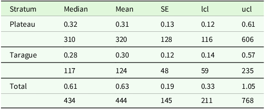
Densities of deer were similar in the Plateau stratum with a mean density of 0.32 deer ha−1 (95% CI = 0.12–0.61; CV = 0.41) and in the Tarague stratum with 0.28 deer ha−1 (95% CI 0.14–0.57; CV = 0.42; Table 1). Deer abundance in the Plateau stratum was 320 individuals (95% CI = 116–606) and in the Tarague stratum it was 124 individuals (95% CI = 59–235). Total deer abundance was 444 individuals (95% CI = 211–768).
Deer population median and mean density (deer ha−1; first row) and abundances (second row) with standard errors (SE) estimates for each stratum and total strata of camera trap records collected in 2022 on the Naval Facilities Engineering System Command Marianas, Andersen Air Force Base, Guam. Bootstrap-derived 95% confidence intervals (lower limit = lcl; upper limit = ucl) are presented. The Plateau stratum was 985 ha and the Tarague stratum 410 ha

There were 4,476 pig detections during the survey period, with 3,712 pig detections in the Plateau stratum and 764 pig detections in the Tarague stratum. The adjustment for temporal activity was 0.35 ± 0.02 (95% CI = 0.32–0.39; CV = 0.06). The hazard rate key model was chosen based on QAIC accounting for overdispersion and left-truncation (Supplementary Material Appendix C Table C2). Visual inspection of diagnostic plots indicated that the model adequately fit the data with greatest deviations in the first bin (Supplementary Material Appendix C Figure C2). The shoulder of the detection function extended out to about 4 m before decaying rapidly. The estimated detection probability of a pig that was within 10.5 m of a camera was 0.270 (SE = 0.005; CV = 0.018).
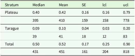
Pigs had substantially higher densities in the Plateau stratum with a mean density of 0.40 pig ha−1 (95% CI = 0.16–0.79; CV = 0.40) than in the Tarague stratum with 0.09 pig ha−1 (95% CI 0.03–0.20; CV = 0.46; Table 2). Pigs abundance in the Plateau stratum was 410 individuals (95% CI = 158–778) and in the Tarague stratum it was 41 individuals (95% CI = 12–83). Total pig abundance was 451 individuals (95% CI = 204–818).
Pigs population median and mean density (pigs ha-1; first row) and abundances (second row) with standard errors (SE) estimates for each stratum and total strata of camera trap records collected in 2022 on the Naval Facilities Engineering System Command Marianas, Andersen Air Force Base, Guam. Bootstrap-derived 95% confidence intervals (lower limit = lcl; upper limit = ucl) are presented. The Plateau stratum was 985 ha and the Tarague stratum 410 ha

Adequate coverage
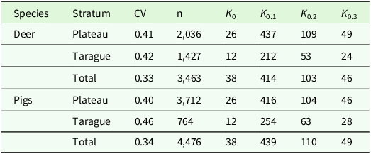
The number of camera trap points required to achieve the target CV values of 0.10, 0.20, and 0.30 varied by species and by strata. The CVs ranged from 0.33 to 0.46 (mean = 0.39 ± 0.05), and estimates of deer densities were slightly more precise in general (i.e., had smaller CVs) than estimates of pig densities (Table 3). In general, precision increased with increasing sampling effort where CVs were largest for estimates in Tarague stratum and lowest for the combined total strata. The number of camera traps required to obtain desired CVs of 0.10 was substantial, requiring increasing of 212 to 439 camera traps. Estimates with CVs of 0.20 are likely still unachievable, ranging from an increase to 53 to 110 camera traps. Roughly doubling the number of camera traps to 24 to 49 would yield CVs of 0.30.
Coefficients of variation (CV), number of detections (n), and number of camera traps deployed (K0) to achieve desired CVs of 0.10, 0.20, and 0.30 (Kest) for deer and pigs by stratum. Values are numbers of camera locations required to achieve target CVs

Discussion
We applied a camera trap survey design based on standard camera trap sampling protocols using motion-activated, videography combined with distance sampling methods to estimate densities of unmarked deer and pigs on the tropical, oceanic island of Guam. We show how CTDS methods can be used to estimate low and high strata-specific abundances and demonstrate that the strata-specific abundances can be combined to provide population-wide estimates (Total estimates; Tables 1 and 2). Our research provides evidence that CTDS methods yield sufficiently accurate and precise estimates for monitoring ungulates and medium-sized animals in tropical environments and Pacific oceanic islands.
Overall, our density estimates of deer and pigs were lower than those of Knutson & Vogt (Reference Knutson and Vogt2002) and Sundance-EA Associates Joint Venture (2020, 2022). Differences in our density estimates were likely due to intensive depredation management efforts where 1,379 deer were removed from both strata in 2021 and 2022 and with more females removed than males (1.39:1 female to male ratio; M Burt, pers. obs.). Within a 33-ha fenced area on Tarague, 15 deer were removed, which is a density of 0.45 deer ha−1 (M Burt, pers. obs.). Our mean estimate of 0.30 deer ha−1 has a relative difference of 33% and our 95% CI of 0.14 to 0.57 deer ha−1 brackets the current population. In 2021 and 2022, 206 pigs were removed from both strata with more females removed than males (1.27:1 female to male ratio; M Burt, pers. obs.). In a 33-ha fenced area on Tarague, 55 pigs were removed, yielding a density of 1.67 pigs ha−1, substantially higher than our estimate of 0.10 pigs ha−1 (94% relative difference) and lies outside our 95% CI of 0.03 to 0.20 pigs ha−1. There was reproduction in the pig population during the year it took to eradicate pigs, which may explain why their estimates were higher (M Burt, pers. obs.). Thus, our lower densities estimated using CTDS are consistent with management activities to reduce ungulate populations. Palencia et al. (Reference Palencia, Rowcliffe, Vicente and Acevedo2021) did not find significant differences in independent and CTDS estimated densities in five out of six multispecies populations but, similar to our results, concluded that CTDS may have underestimated densities of wild pigs in the sixth population. Cappelle et al. (Reference Cappelle, Després-Einspenner, Howe, Boesch and Kühl2019) and Harris et al. (Reference Harris, Butler, Stewart, Rominger and Ruhl2020) both compared CTDS estimates against populations of known size and estimates were consistent with true abundances. Although the simulation and duiker studies of Howe et al. (Reference Howe, Buckland, Despres-Einspenner and Kühl2017) and multispecies study of Palencia et al. (Reference Palencia, Rowcliffe, Vicente and Acevedo2021) are not definitive, they indicate a consistency of CTDS methods to estimate unbiased densities of unmarked populations.
Our camera trap survey design provided relatively precise densities of both deer and pigs simultaneously, with CVs of 0.33 to 0.46 (Table 3). CTDS yielded similar CVs for western chimpanzees (0.40; Cappelle et al. Reference Cappelle, Després-Einspenner, Howe, Boesch and Kühl2019). Our CVs were comparable with or slightly smaller than CVs for bighorn sheep (mean = 0.58 ± 0.13; range = 0.42 to 0.75; Harris et al. Reference Harris, Butler, Stewart, Rominger and Ruhl2020), were slightly larger than CVs for marmot (0.28; Corlatti et al. Reference Corlatti, Sivieri, Sudolska, Giacomelli and Pedrotti2020), were similar to the mean CV of a community of rainforest species (mean = 0.36 ± 0.15; range = 0.17 to 0.71; Bessone et al. Reference Bessone, Kühl, Hohmann, Herbinger, N’Goran, Asanzi, Da Costa, Dérozier, Fotsing, Beka, Iyomi, Iyatshi, Kafando, Kambere, Moundzoho, Wanzalire and Fruth2020) and to CVs of group-living and solitary mountain ungulates (mean = 0.39 ± 0.06; range = 0.34 to 0.48; Pal et al. Reference Pal, Bhattacharya, Qureshi, Buckland and Sathykumar2021). Increasing the number of camera trap sites may be necessary to improve precision to determine harvesting regimes or to demonstrate the effectiveness of management activity. Guidance on determining spacing among camera traps for CTDS methods is limited, but in general spacing is relatively flexible. Most uncertainty in CTDS population estimates is derived from the encounter rate variation due to the small size of the area monitored at a camera trap site (i.e., the FOV; Howe et al. Reference Howe, Buckland, Despres-Einspenner and Kühl2019, Cappelle et al. Reference Cappelle, Howe, Boesch and Kühl2021). Howe et al. (Reference Howe, Buckland, Despres-Einspenner and Kühl2017) showed that increasing locations improved precision, and Bessone et al. (Reference Bessone, Kühl, Hohmann, Herbinger, N’Goran, Asanzi, Da Costa, Dérozier, Fotsing, Beka, Iyomi, Iyatshi, Kafando, Kambere, Moundzoho, Wanzalire and Fruth2020) achieved many locations by moving cameras. A high-density grid better captures the heterogeneity among trap sites than a low-density grid leading to reduced encounter rate variation and more precise abundance estimates. To reduce the required number of cameras to sample all points on a high-density grid, Palencia et al. (Reference Palencia, Rowcliffe, Vicente and Acevedo2021) noted that using a moving survey approach where camera traps are deployed in one subset of the grid (e.g., every other point) and are then moved to a new location (e.g., the remaining points) will increase the sampled locations and in consequence increase precision. In our study, we rotated the orientation of each camera on a low-density grid to increase sample sizes and better capture microsite heterogeneity. We detected nearly twice as many deer and almost four times as many pigs when cameras were oriented south (2,082 and 3,031, respectively) than detected when cameras were oriented north (1,176 and 783, respectively), indicating that there was substantial microsite heterogeneity in detections of both deer and pigs. Hofmeester et al. (Reference Hofmeester, Cromsigt, Odden, Andrén, Kindberg and Linnell2019) showed that microsite conditions influence animal detection and concluded that microsite factors are probably most important for camera trap sampling. Rotating camera orientation will likely be more efficient than finding new suitable trees, and rotation of cameras can be accomplished when visiting the trap sites to replace batteries and SD cards during the survey. Greater numbers of camera traps would be needed to achieve desired levels of precision, generally doubling to quadrupling the number of camera trep sites to achieve CVs of 0.3 and 0.2, respectively. Thus, incorporating a high-density grid providing greater coverage may be necessary to evaluate management activities.
Density and abundance estimates using distance sampling methods are unbiased when critical assumptions are met (Buckland et al. Reference Buckland, Rextad, Marques and Oedekoven2015). For CTDS, assumptions are that the detectors are randomly located relative to animals distribution and density, animals at distance 0 are perfectly detected, distances are measured accurately, animals are detected at their initial location, and animal movement is not altered by detection (Buckland et al. Reference Buckland, Anderson, Burnham, Laake, Borchers and Thomas2001, Reference Buckland, Rextad, Marques and Oedekoven2015, Howe et al. Reference Howe, Buckland, Despres-Einspenner and Kühl2017). The first four assumptions can be achieved with a robust study design and sampling procedures. The assumption that animal movement is unaltered can be violated by attraction to or avoidance of camera traps. This assumption can also be violated if animals react to cameras by changing their speed of movement. Animals slowing down or freezing while in the FOV yields more detections at snapshot moments than if the animal moved at a speed unaffected by the camera. CTDS estimates are unbiased only when the study species is active and all animals are available for detection (Rowcliffe et al. Reference Rowcliffe, Kays, Kranstauber, Carbone and Jansen2014, Howe et al. Reference Howe, Buckland, Despres-Einspenner and Kühl2017). The temporal availability approach we used was to multiply densities by the proportion of time when animals are available (Howe et al. Reference Howe, Buckland, Despres-Einspenner and Kühl2017; Nakashima et al. Reference Nakashima, Fukasawa and Samejima2018), and a best practice is to estimate temporal availability for each camera trap study to avoid study-specific availability bias. In Supplementary Material Appendix D, we provide study design and sampling procedure points to consider when using CTDS methods to monitor populations; researchers can use these best-practice points to expand the use of CTDS methods to new locations and taxa.
We demonstrated that CTDS is useful where management actions of intense control efforts are implemented, and we conclude that the method is particularly well-suited to estimating densities of ungulates on oceanic islands. Due to lack of predators and an abundance of suitable habitat, deer and pigs occur at fairly high densities (Hess Reference Hess2016), which facilitates quickly obtaining sufficient numbers of detections to accurately estimate population size. Even when ungulates occur at low densities due to control actions, such as on Tarague where we estimated 124 deer and 41 pigs (Tables 1 and 2), we showed CTDS can still be used to generate population estimates. Facilitating detection of ungulates with CTDS is that their herbivorous and habitat generalist nature makes them more widespread than ambush predators or habitat specialists, potentially reducing the encounter rate variance among camera traps, and thus reducing CVs. The large body size of ungulates means they are likely to reliably trigger the camera traps, so the critical CTDS assumption of perfect detection at 0 distance is very likely to be met (Rowcliffe et al. Reference Rowcliffe, Kays, Kranstauber, Carbone and Jansen2014, Howe et al. Reference Howe, Buckland, Despres-Einspenner and Kühl2017). Due to their stature, deer and pigs occur within the vertical range of camera traps, and the assumption that they are available for detection can be met (Rowcliffe et al. Reference Rowcliffe, Kays, Kranstauber, Carbone and Jansen2014, Howe et al. Reference Howe, Buckland, Despres-Einspenner and Kühl2017). A potential source of bias in CTDS comes from animals reacting to the camera traps, and when animals react to cameras being triggered. We observed some individuals appeared to respond to the camera traps, quickly moving out of the FOV after the camera triggered. This occurred infrequently enough such that it is reasonable to assume points remain independent of animal density and distribution, and it is not necessary to censor many detections. Our research provides evidence extending CTDS methods to tropical Pacific oceanic islands and corroborates that the method is useful for monitoring ungulates and medium-sized animals in tropical environments.
Supplementary material
The supplementary material for this article can be found at https://doi.org/10.1017/S0266467425000033
Data availability
The video imagery analysed in this study is available on request from NAVFACMAR (Naval Facilities Engineering Systems Command Marianas).
Acknowledgements
We thank Matt Kedziora, Natural Resources Specialist, NAVFACMAR, Navy Base Guam, for providing the 14 Bushnell Trophy Cameras and Mike Park, Natural Resources Specialist, Andersen Air Force Base Guam, for assistance with camera deployment, reorientation, and retrieval. We thank Eric Howe, Ontario Ministry of Natural Resources and Forestry, and Anna Staudenmaier, Commonwealth of the Northern Mariana Islands Department of Land and Natural Resources, for discussions on camera trap distance sampling methods and analysis. We thank Derek Risch, University of Hawai‘i at Mānoa, and two anonymous reviewers for helpful comments on an early draft. Any use of trade, product, or firm names in this publication is for descriptive purposes only and does not imply endorsement by the U.S. Government.
Competing interests
The authors declare none.
Financial support
Funding was provided by the U.S. Navy (Commander, Navy Installation Command, NAVFACMAR) grant #N4155721MP001GE and U.S. Geological Survey Invasive Species Program.
Ethical statement
This was an observational study; thus, no animals were handled in accordance with animal welfare standards of the University of Hawai‘i Institutional Animal Care and Use Committee.