1. Introduction
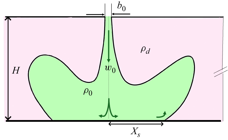
Turbulent fountains constitute a special case of buoyant jets when the momentum flux at the source is supplied in a direction opposite to that of the buoyancy flux (List Reference List1982). They are classified as ‘free’ if no solid boundaries are present in their vicinity, and the flow is allowed to develop for significantly large streamwise distances compared with its characteristic dimension. Meanwhile, for an ‘impinging’ fountain, the presence of a solid wall orthogonal to the propagation direction significantly alters the flow physics, especially in the near-wall region (Cooper & Hunt Reference Cooper and Hunt2007; Srinarayana, Armfield & Lin Reference Srinarayana, Armfield and Lin2009; Hunt & Burridge Reference Hunt and Burridge2015). They are deemed significant to the geophysical fluid dynamics community as well as to the industry (Baines, Turner & Campbell Reference Baines, Turner and Campbell1990; Bloomfield & Kerr Reference Bloomfield and Kerr2000; Mingotti & Woods Reference Mingotti and Woods2016). Figure 1(a) shows a schematic of an impinging fountain that is discharged in a uniform ambient (UA) of higher density. The primary aim of the present work is to investigate how the presence of a lateral density difference, such as that shown in figure 1(b), will affect the structural and dynamical aspects of an impinging line fountain. The subscripts d and l have been used to represent dense and light fluids, respectively. Physically, this lateral density stratification imposes a gravity-driven bidirectional cross-flow and adds unique characteristics to the fountain development, which is not very well understood. This bidirectional lateral forcing significantly affects the trajectory and results in a asymmetry in the fountain spread as shown in the schematic in figure 1(c). Such configurations find direct application in building flows, e.g. when temperature sharply changes across a doorway opening, and air curtains are installed to restrict the fluid exchange (Hayes & Stoecker Reference Hayes and Stoecker1969; Frank & Linden Reference Frank and Linden2014). Similarly, in the coastal regions, bubble screens are installed underwater to prevent mixing of freshwater with saline water that is largely driven by a horizontal forcing (Oldeman et al. Reference Oldeman, Kamath, Masterov, O’Mahoney, van Heijst, Kuipers and Buist2020; Bacot, Frank & Linden Reference Bacot, Frank and Linden2022). Previous studies that have considered this density arrangement (Guyonnaud et al. Reference Guyonnaud, Solliec, Dufresne de Virel and Rey2000; Jha, Frank & Linden Reference Jha, Frank, Darracq and Linden2021a , Reference Jha, Frank and Lindenb ; Frank et al. Reference Frank, Jha, Koene, Kemp, Twerda and Linden2022; Agrawal et al. Reference Agrawal, Agarwal, Chalamalla and Jha2023a , Reference Agrawal, Jha and Chalamallab ) largely focused on the bulk fluid exchange between the dense and light sides and quantified a separation efficiency. However, to the best of our knowledge, a detailed investigation probing the underlying velocity and entrainment dynamics remains due.
Fountains are typically characterized using a Froude number,
 $Fr{_0} = {w{_0}}/{\sqrt {g^\prime b{_0}}}$
(Kaye & Hunt Reference Kaye and Hunt2006; Williamson, Armfield & Lin Reference Williamson, Armfield and Lin2011; Hunt & Burridge Reference Hunt and Burridge2015). Here
 $g^\prime = {g(\rho _{d} - \rho {_0})}/{\rho {_0}}$
is the reduced gravity between the source fluid and its ambient. Here
 $b{_0}$
and
 $w{_0}$
denote the width and the exit velocity of the fountain. In the case of impinging fountains, the geometric ratio
 $H/b_0$
also plays an important role as was shown by Cooper & Hunt (Reference Cooper and Hunt2007) for axisymmetric fountains and Srinarayana et al. (Reference Srinarayana, Armfield and Lin2009) for line sources. Here,
 $H$
represents the distance between the fountain exit and the impingement surface as shown in figure 1. Cooper & Hunt (Reference Cooper and Hunt2007) reported that a buoyant radial wall jet develops near the wall after the fountain impinges. This wall jet spreads radially until a distance
 $R_{s}$
and separates once the buoyancy force overcomes the Coanda effect (see figure 1
a). A significant fraction of this fluid is then re-entrained into the radial wall jet and the fountain, resulting in the formation of a toroidal vortex. Based on theoretical arguments and subsequently supported by laboratory measurements, they obtained the scaling
 ${R_{s}}/{H} = 0.03 \textit{Fr}_0^{3/2}$
for the maximum non-dimensional radial spread with the source Froude number. The corresponding case of line fountains was studied using direct numerical simulation by Srinarayana et al. (Reference Srinarayana, Armfield and Lin2009) for 50
 $\leqslant Re \leqslant$
1000, and 8
 $\leqslant \textit{Fr}_0 \leqslant$
20, where
 $\textit{Re} = w_0b_0/\nu$
. The ceiling height,
 $H$
, was varied between 10
 $b_0$
and 30
 $b_0$
in their simulations. The normalized lateral spreading distance after the impingement
 $({H + X_{s}})/{b_0}$
was shown to scale as
 $\textit{Fr}_0^{2/3} \sqrt {{H}/{b_0}}$
for all values of Froude numbers considered. For larger
 $H/b_0$
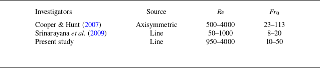
, their direct numerical simulation demonstrated an asymmetric flow development with an intermittent flapping of the fountain core. Table 1 highlights that the current literature on impinging line fountains is restricted to the quantification of lateral spread at low to moderate Froude number. Therefore, the secondary objective of the present work is to extend the range of Froude number for these fountains, and to investigate their flow statistics and entrainment characteristics, which will lead to a better understanding of the rich and complex flow physics of impinging line fountains. By definition, the Froude number does not explicitly consider a density difference across the fountain in the horizontal direction. Therefore, it cannot be used to completely characterize the impinging fountains subjected to a lateral density stratification. The existing literature on buoyant jets being discharged in a cross-flow usually employs a velocity ratio,
 $V_r$
, for their characterization (Smith & Mungal Reference Smith and Mungal1998; Muppidi & Mahesh Reference Muppidi and Mahesh2005; Mahesh Reference Mahesh2013; Pokharel & Acharya Reference Pokharel and Acharya2021). Here
 $V_r$
compares the relative magnitude of the average discharge velocity at the source
 $w_0$
with respect to that of the cross-flow. In these cases, however, the cross-flow is generally unidirectional and externally imposed, for example, due to a boundary layer developing in a channel or a uniform free stream. In comparison, the present configuration inherently enforces a gravity-driven bidirectional cross-flow (Simpson Reference Simpson1982; Sher & Woods Reference Sher and Woods2017) that is fundamentally different to the previously studied problems. Therefore, we use another non-dimensional parameter, known as the deflection modulus (
 $D{_m}$
) that has previously been used to characterize air curtains and bubble screens (Hayes & Stoecker Reference Hayes and Stoecker1969; Frank & Linden Reference Frank and Linden2014; Jha et al. Reference Jha, Frank and Linden2021b
; Bacot et al. Reference Bacot, Frank and Linden2022). Here
 $D{_m}$
compares the momentum flux of the source fluid with the stack effect that is imposed by the lateral buoyancy. Mathematically, it is given as
 \begin{equation} D{_m} = \frac {\rho _{_0} b_{_0} w_{_0}^2}{g (\rho _{_d} - \rho _{_l}) H^2}. \end{equation}
Noticeably, the deflection modulus includes the length scales associated with the fountain source (
 $b_0$
) as well as the source-plate separation (
 $H$
), while also considering the lateral density difference between
 $\rho _{_d}$
and
 $\rho _{_l}$
.
Comparison of source conditions for studies investigating impinging fountains in a UA for
 $H/b_0 \geqslant$
10.

(a) General schematic of an impinging fountain in a uniform calm ambient, (b) gravity-driven bidirectional cross-flow and (c) impinging fountain in this cross-flow. Subscripts
 $d$
and
 $l$
corresponds to dense and light fluids, respectively. Arrows in (b) represents the variation of hydrostatic pressure.

The paper is organized as follows. Sections 2.1 and 2.2 describe the numerical simulations and laboratory measurements conducted in this study, respectively. Section 3.1 presents the effect of lateral stratification on the general structure of fountains. Quasisteady fields are analysed in § 3.2 to quantify lateral deflection as well as the mean and turbulent velocity statistics. The entrainment coefficient is formally estimated in § 3.3 to quantify mixing of ambient fluid with the fountains. The major conclusions are summarized in § 4.
2. Methodology
The present study uses data obtained from numerical computations and laboratory measurements. Three-dimensional spatiotemporal fields of velocity and density are obtained using large-eddy simulation (LES) whereas time-resolved particle image velocimetry (TR-PIV) measurements provide velocity information to quantify the statistical characteristics of these line fountains.
2.1. Numerical simulations
The primary mode of investigation in the present study is to use the high-fidelity data obtained from the LES simulations conducted using the stratified ocean model with adaptive refinement (SOMAR), developed at University of North Carolina (Santilli & Scotti Reference Santilli and Scotti2015; Chalamalla et al. Reference Chalamalla, Santilli, Scotti, Jalali and Sarkar2017). A spatial filtering operation, that distinguishes the large or the resolved scales from their smaller or subgrid counterparts, is inherent to any LES computation. In our numerical model, we solve the following set of filtered governing equations under the Boussinesq approximation, assuming a linear equation of state for density:
 \begin{equation} \frac {\partial {\overline {u}_i}}{\partial {x_i}}=0, \end{equation}
 \begin{equation} \frac {\partial \overline {u}_i}{\partial t} + \overline {u}_{\!j}\frac {\partial {\overline {u}_i}}{\partial {x_{\!j}}} = - \frac {1}{\rho _0} \frac {\partial {\overline {p}}}{\partial {x_i}} - {{\overline {g^\prime }}} \ \delta _{i3} + \frac {\partial }{\partial {x}_{\!j}}\left (\nu \frac {\partial {\overline {u}_i}}{\partial {x}_{\!j}}-\tau ^R_{\textit{ij}}\right )\!, \end{equation}
 \begin{equation} \frac {\partial \overline {g^\prime }}{\partial t} + \overline {u}_{\!j}\frac {\partial {\overline {g^\prime }}}{\partial {x_{\!j}}} = \kappa _b \frac {\partial }{\partial {x}_{\!j}}\left (\frac {\partial {\overline {g^\prime }}}{\partial {x}_{\!j}}-\lambda ^R_{j}\right )\!. \end{equation}
Equations (2.1), (2.2) and (2.3) physically represent the conservation laws associated with mass, momentum and buoyancy. In these equations,
 $\overline {u}_i$
denotes the ith component of filtered velocity field and
 $\overline {g^\prime } = g \overline {\rho }/\rho _0$
is the filtered buoyancy field. Here,
 $\overline {p}$
indicates the corresponding pressure and
 $\rho _0$
is the reference density. Kinematic viscosity is denoted by
 $\nu$
whereas
 $\kappa _b$
represents scalar diffusivity. The subgrid scale stresses and buoyancy fluxes are given as
 $\tau ^R_{\textit{ij}}$
and
 $\lambda ^R_{\textit{ij}}$
, respectively. An eddy-viscosity-based approximation is used to model the anisotropic component of the subgrid stress tensor,
 $\tau _{\textit{ij}}^R = \rho \overline {u_i u_{\!j}} - \rho \overline {u}_i \overline {u}_{\!j}$
, and the subgrid buoyancy flux,
 $\lambda ^R$
as
 \begin{equation} \tau ^R_{\textit{ij}} - \frac {1}{3}\tau ^R_{kk}\delta _{\textit{ij}} = -2 \nu _{\textit{sgs}} \overline {S}_{\textit{ij}}, \end{equation}
 \begin{equation} \lambda _{\!j}^R = -2 \kappa _{\textit{sgs}} \frac {\partial \overline {g^\prime }}{\partial x_{\!j}}. \end{equation}
In the above relation,
 $\overline {S}_{\textit{ij}}$
denotes the strain rate associated with the filtered velocity field. The subgrid-scale Prandtl number, denoted as
 $\textit{Pr}_{\textit{sgs}} = \nu _{\textit{sgs}}/\kappa _{\textit{sgs}}$
, has been assumed as unity for all the LES simulations reported. The SOMAR uses a second-order finite difference scheme for the spatial discretization of various gradients, and the time stepping has been done using the RK3 method.
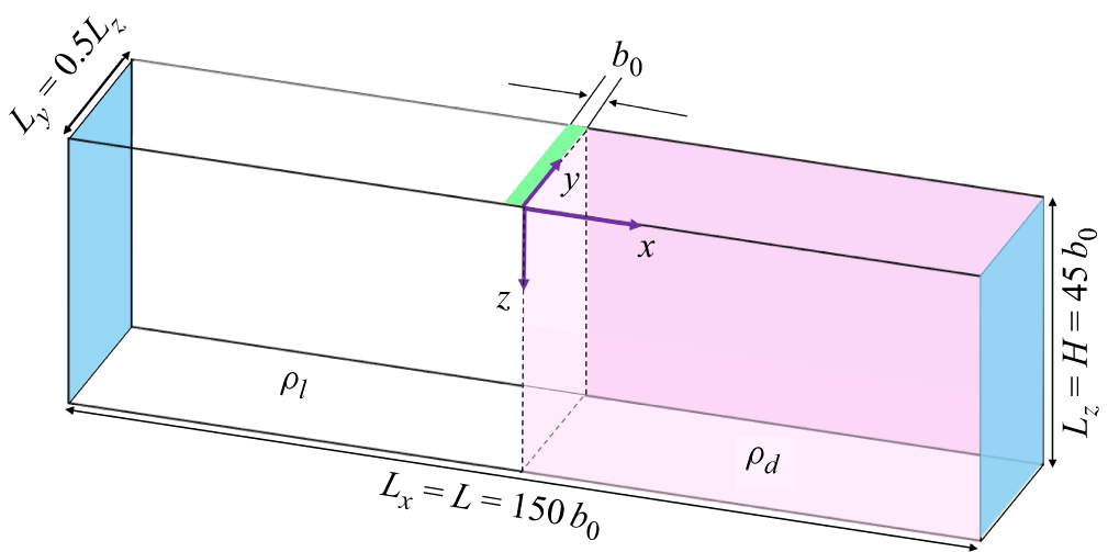
Computational schematic of fountain in laterally stratified ambient (LSA) at
 $t =$
0.

These computations are performed in a box of size 150
 $b_0 (L) \ \times$
22.5
 $b_0 (W)\ \times$
45
 $b_0 (H)$
, where
 $b_0$
is the total width of planar source at the exit, as shown in figure 2. We use water as the working fluid to ensure dynamic similarity (Linden Reference Linden1999) and to maintain consistency with the experiments. The numerical results are later validated against the data obtained from laboratory measurements. In order to create the necessary stratification in the domain, SOMAR has capabilities to incorporate temperature as well as salinity variations in the linearized equation of state, and the associated governing equations. In the simulations reported and experiments that are described later, we use a salinity inhomogeneity to alter the fluid properties and induce the desired density difference.
Initially, the regions
 $ [-({L_x}/{2}), 0 ]$
and
 $ (0, ({L_x}/{2}) ]$
of the computational domain are assigned a salinity level of
 $S_l =$
0 and
 $S_d \neq$
0, respectively. Here, the subscripts
 $l$
and
 $d$
imply light and dense fluid, respectively (see figure 2). To simulate a UA, the entire domain is initially filled with fluid corresponding to
 $S_d \neq$
0. The source of the line fountain (shown in green) is located between
 $[-b_0,0]$
and occupies the total spanwise extent (
 $L_y$
) of the computational domain, resulting in a nearly two-dimensional flow development. A uniform top-hat velocity profile with magnitude
 $w_0$
is supplied such that the resultant Reynolds number,
 $\textit{Re} = {b_0 w_0}/{\nu }$
, at the exit plane is 4000 for all the simulations ensuring turbulent fountains. The source salinity,
 $S_0$
, is taken equal to that of
 $S_l = 0$
for both the cases, to obtain a positively buoyant system where momentum is advertently opposed by buoyancy. End walls, shown in blue in figure 2, are imposed with zero shear boundary condition to facilitate an outflow to ensure mass continuity inside the computational box. All other walls in the flow domain are treated as no-slip, and no-penetration boundaries. A detailed description of the computational grid is provided in our previous study (Agrawal et al. Reference Agrawal, Jha and Chalamalla2023b
), which is also summarized in Appendix A.
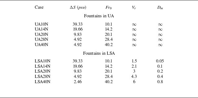
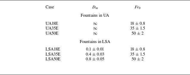
Table 2 presents the various cases studied in the present work. The simulations reported have been conducted for at least 20 flow through times (
 $H/w_0$
) with the corresponding time step,
 $\Delta t$
, obeying the Courant–Friedrichs–Lewy criterion (Ferziger, Perić & Street Reference Ferziger, Perić and Street2019) such that the resulting Courant–Friedrichs–Lewy number remains less than 0.8 in the entire computational domain at all times. Froude number at the exit,
 $\textit{Fr}_0$
, indicates that the fountains under consideration are highly forced (Hunt & Coffey Reference Hunt and Coffey2009). The corresponding value of Richardson number,
 $Ri_0 = {g^\prime b_0}/{w_0^2} = {1}/{\textit{Fr}_0^2}$
, although not given in table 2, can also be evaluated. The range of
 $Ri_0$
in the present simulations is between 0.0003 and 0.01. Other than the deflection modulus, table 2 also lists the velocity ratio,
 $V_r$
, that is typically employed for studying jets in cross-flow. We use the buoyancy velocity scale
 $w_{_B} = \sqrt {g^\prime H}$
to characterize the cross-flow, and thus,
 $V_r = {w_0}/{\sqrt {g^\prime H}}$
. At low velocity ratios, counter-rotating vortex pair populate the wake region of the flow, and their formation is delayed upon increased
 $V_r$
(Smith & Mungal Reference Smith and Mungal1998; Mahesh Reference Mahesh2013).
Large-eddy simulations conducted in the present study. The numbers in the case name are related to the source Froude number,
 $\textit{Fr}_0$
, and the last letter, ‘N’, indicates numerical simulations.

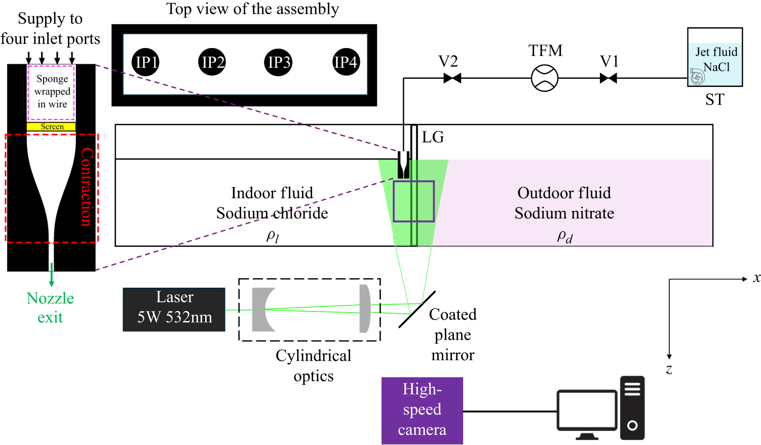
Schematic of the experimental set-up at the instant before removing the LG.

2.2. Experimental details
Experiments have also been conducted in parallel to study the dynamics of line fountains developing in a UA as well as under cross-flow conditions obtained using a lateral density stratification. A glass tank of length,
 $L =$
2 m, width,
 $W =$
0.18 m and height,
 $H_T =$
0.4 m, as shown in figure 3, is used for this purpose. In all the measurements, the fluid level was kept at
 $H =$
0.1 m, unless stated otherwise. Before an experiment commences, the tank is divided into two parts using a Perspex sheet (lock gate (LG)) installed in the centre which spans across the entire width of the tank. Thereafter, one side of the tank is filled with an aqueous sodium chloride (NaCl) solution of predetermined concentration resulting in the density associated with the light fluid in the system,
 $\rho _l$
. At the same time, the other side is supplied an aqueous sodium nitrate (NaNO
 $_3$
) solution of density
 $\rho _d$
. For the facilitation of optical investigation and to avoid anomalies associated with particle blurring in the PIV images, the refractive index,
 $n$
, of the two solutions are carefully matched as detailed in Appendix B. In the experiments reported, we measured the corresponding values of
 $n$
using the Atago PAL-RI refractometer (accuracy:
 $\pm$
0.0003).
Experiments conducted in the present study. The numbers in the case name are related to the source Froude number,
 $\textit{Fr}_0$
, and the last letter, ‘E’, indicates experimental datasets. The notation
 $D_m = A \pm B$
represents
 $A$
as the nominal value with
 $B$
as the variation in
 $A$
across the ensemble of multiple repetitions.

The planar nozzle employed in the experiments is fabricated from a Teflon block which was CNC (computer numerical control) machined to produce a rectangular slot of dimension
 $l_0 =$
0.166 m and
 $b_0 =$
0.002 m, resulting in an aspect ratio of 83. To ensure even dispersal of the incoming supply fluid along the span of the slot, four inlet ports (IP1, IP2, IP3, IP4) are provided along the length of the inlet manifold, as shown in the top view of the nozzle assembly in figure 3. In the flow conditioning chamber, a fine sponge encased in a flexible steel wire mesh is inserted to allow a uniform redistribution of the supply fluid. An acrylic screen, shown as yellow, with an area blockage ratio of 85 % is also provided for further smoothing of the incoming supply. Following the conditioning section, the fluid then enters a contraction with an area ratio of 9 which is marked as red in figure 3. The design of the contracting chamber is based on a fifth-order polynomial as outlined by Mehta & Bradshaw (Reference Mehta and Bradshaw1979). An additional length of 15 mm (7.5
 $b_0$
) is provided before the fluid finally exits through the rectangular slot resulting in a line fountain. The reservoir for the source fluid is an aqueous sodium chloride solution of essentially the same concentration and refractive index as that of the lighter fluid, and is denoted as ST in the schematic. This fluid is supplied through a centrifugal pump, the delivery head of which is regulated using a control valve, V1. The measurement of flow rate through the nozzle is done using a turbine flowmeter (TFM) with an accuracy of
 $\pm$
1 %. An additional control valve, V2, is used to fine-tune the flow rate through the nozzle to a predetermined value of
 $Q_0 =$
8.5 litres per minute used across all the experiments. Throughout the experimental run time, which is typically of the order of 60 s, we monitor
 $Q_0$
and observe the fluctuations to be within 3 %. The measured Reynolds number,
 $\textit{Re} = {w_0 b_0}/{\nu }$
is approximately 1000 for all the present experiments, thereby indicating a fully turbulent flow. Table 3 lists the set of experiments conducted in the present study. Details pertaining to conducting a typical experiment and acquiring PIV images are presented in Appendix C.
3. Results
This study first explores the evolution of turbulent fountains, revealing that lateral buoyancy induces an inclination dependent on the density difference,
 $\Delta \rho$
(§ 3.1). Next, we analyse the fountain’s lateral deflection and velocity statistics, comparing its decay and spreading rates with the UA counterpart (§ 3.2). Finally, we estimate the entrainment coefficient from integral flux measurements (§ 3.3).
3.1. Transient flow development
We first examine the transient development of flow fields obtained through numerical simulations. The general structure of line fountains is discussed in §§ 3.1.1 and 3.1.2 for lower and higher deflection modulus, respectively. An analytical model is presented in § 3.1.3 that provides an expression for the post-impingement lateral spread.
Pseudocolour contour plots from the LES data showing the spatiotemporal evolution of the normalized scalar concentration in fountains being discharged in a UA (case UA14N:
 $\textit{Fr}_0$
= 14.2 in panels (a), (c) and (e)). Panels (b), (d) and ( f) presents the corresponding scalar distribution for a fountain evolving in a LSA (case LSA14N:
 $\textit{Fr}_0$
= 14.2,
 $D_m$
= 0.1).

3.1.1. Effect of lateral stratification: deflecting fountains (
 $D_m \lessapprox$
0.1)

We will first show the temporal evolution of line fountains in a UA (case UA14N:
 $\textit{Fr}_0$
= 14.2), and compare it with the corresponding development in a LSA (case LSA14N:
 $\textit{Fr}_0$
= 14.2,
 $D_m$
= 0.1). This comparison is performed at smaller values of
 $D_m$
to provide useful qualitative insights into the flow field development and the associated changes induced due to the cross-stream buoyancy. Figure 4 shows the spatial distribution of the normalized scalar field (
 $c_{\!j} = c/c_0$
) in the
 $x{-}z$
midplane at various time instants providing information pertaining to the structure and integrity of these fountains. At
 $t =$
0, the scalar concentration (
 $c$
) is set as zero in the entire computational domain. Whereas, the value of source concentration (
 $c_0$
) has been taken as unity at the fountain exit. Panels in the left and right columns in figure 4 correspond to UA (UA14N) and LSA (LSA14N) cases, respectively.
Figures 4(a) and 4(b) clearly illustrate the effect of lateral density stratification on the fountain structure. While the uniformly dense ambient decelerates the source fluid, the trajectory of the UA14N fountain (figure 4
a) remains vertical. In comparison, the cross-stream density difference in case LSA14N exerts a lateral force on the fountain resulting in a significant inclination with respect to the vertical. This inclination is seen to be higher at lower-
 $D_m$
(or equivalently, lower-
 $\textit{Fr}_0$
) and is later quantified in § 3.2.1. Due to this deflection, the fountain core exhibits a lateral shift in the +ve
 $x$
-direction as shown in figure 4(b). At small values of
 $D_m$
, the initial vertical momentum of the source fluid is largely converted into a lateral flow that further interacts with the gravity current that generates due to the lateral density stratification. Figure 4(d) shows such an interaction where the fountain fluid is transported by the advecting gravity current. Interestingly, this transport occurs in a direction opposite to that of the primary orientation of the fountain. The ambient of UA14N provides a completely different mechanism for further evolution of the fountain. Since a UA does not support the formation of gravity currents, the lateral extent of the fountain is largely dictated by the strength of opposing buoyancy. Figure 4(c) depicts that once the fountain impinges, the source fluid may not possess sufficient momentum to continue along the impingement surface and could be significantly influenced by buoyancy. In the present simulations, the impingement did not occur for the case UA10N as the source Froude number (
 $\textit{Fr}_0 = 10.1$
) resulted in a momentum length scale smaller than the domain height,
 $H$
(Frank & Linden Reference Frank and Linden2015; Parker et al. Reference Parker, Burridge, Partridge and Linden2020). After impingement, the buoyant fluid then constitutes an upward return flow around the downward blowing fountain as indicated in figure 4(e). This returning fluid interacts with the fountain fluid on one side, and the denser ambient on the other. The overall lateral width of the line fountain near the impingement surface is governed by the source Froude number, which is later described in more details in § 3.1.3. On the other hand, the source fluid in case LSA14N continues to be deflected sideways due to the lateral density stratification as shown in figure 4( f). Since the source fluid is inherently buoyant in nature, it accumulates near the upper boundary of the computational domain in an asymmetric manner. This asymmetry is a key differentiating structural feature that affects the fountain trajectory as well as the scalar distribution when these fountains evolve in a LSA.
3.1.2. Effect of lateral stratification: impinging fountains (
$D_m \gtrapprox$
0.1)

The previous section discussed the transient evolution of line fountains discharged in uniform and laterally stratified surroundings at low
 $\textit{Fr}_0$
(or
 $D_m$
). For the same source Froude number, the presence of cross-stream density difference resulted in a complete lateral deflection leading to asymmetrical fluid accumulation. The implications of a weaker lateral stratification would be considered now. Figure 5 shows the distributions of normalized scalar in the
 $x{-}z$
centreplane for case UA28N (UA,
 $\textit{Fr}_0$
= 28.4) in figure 5(a,c,e) and compare it with the development in case LSA28N (LSA,
 $\textit{Fr}_0$
= 28.4,
 $D_m$
= 0.4) in figure 5(b,d, f).
Pseudocolour contour plots from the LES data showing the spatiotemporal evolution of the normalized scalar concentration in fountains being discharged in a UA (case UA28N:
 $\textit{Fr}_0$
= 28.4 in panels (a), (c) and (e)). Panels (b), (d) and ( f) presents the corresponding scalar distribution for a fountain evolving in a LSA (case LSA28N:
 $\textit{Fr}_0$
= 28.4,
 $D_m$
= 0.4).

Figure 5(a) depicts that the higher-
 $\textit{Fr}_0$
fountain in a uniformly calm ambient (UA28N) reaches the impingement surface, whereas, in the presence of a lateral stratification, the fountain fluid is forced to travel along a longer path as evident from the inclined trajectory in figure 5(b). The primary structural difference between the cases LSA14N (
 $\textit{Fr}_0 = 14.2$
in figure 4
b) and LSA28N (
 $\textit{Fr}_0 = 28.2$
, in figure 5
b) results from the latter’s ability to counter the gravity current that is generated due to the lateral density difference. Therefore, the LSA28N fountain (
 $D_m = 0.4$
) impinges, albeit at an angle on the bottom wall. This is consistent with the previous work on air curtains who obtained a critical value of
 $D_m \approx 0.125$
for optimized sealing (Hayes & Stoecker Reference Hayes and Stoecker1969; Guyonnaud et al. Reference Guyonnaud, Solliec, Dufresne de Virel and Rey2000; Frank & Linden Reference Frank and Linden2014; Agrawal et al. Reference Agrawal, Jha and Chalamalla2023b
). Upon impingement of the fountains that are discharged in a UA (UA28N), buoyant wall jets are formed on either side that propagate in opposite directions as shown in figure 5(c). Fluid in the impinging fountain constitutes the ‘source’ of these buoyant wall jets. As they travel laterally along the impingement surface, their momentum gradually reduces owing to the opposing buoyancy and viscous effects. Once their momentum is completely exhausted, the buoyant fluid lifts up after reaching a certain spreading distance as indicated in figure 5(e). This lateral spread is governed by the source
 $\textit{Fr}_0$
and the geometric ratio
 $H/b_0$
, and is discussed in more details in the next section. In comparison, the impingement of fountains in LSA results in the generation of asymmetric wall jets. On one side where the source fluid experiences an opposing buoyancy, a buoyant wall jet is formed similar to the case UA28N. However, the other side where the density of the fountain fluid matches to that of the ambient, essentially results in a non-buoyant wall jet as shown in figure 5(d). The propagation characteristics of the two wall jets are also noticeably different with the non-buoyant wall jet travelling faster than its buoyant counterpart. This results in a larger lateral spread on the non-buoyant side (indicated by
 $X_{_{\textit{S}\text{,}\textit{NB}}}$
) as compared with the buoyant half
 $X_{_{S,B}}$
. Quantifying these spreads are important for design consideration in engineering applications. For instance, the air curtains must be operated such that the lateral span of the buoyant wall jet is small in comparison with the building dimension. This would restrict the spatial extent of mixed fluid that the buoyant wall jet may bring inside a building.
3.1.3. A model for the lateral spread
In this section, we derive an analytical expression for the lateral spread,
 $X_S$
, when a line fountain impinges in a UA. Consider the schematic shown in figure 6, we define the fluxes of volume (
 $Q_0$
), momentum (
 $M_0$
) and the buoyancy (
 $B_0$
) at the source as
 \begin{align} Q_0 & = b_0w_0 , \\[-12pt]\nonumber \end{align}
 \begin{align} M_0 & = b_0w_0^2 , \\[-12pt]\nonumber \end{align}
 \begin{align} B_0 & = g^\prime _0Q_0. \end{align}
Schematic of a line fountain of density
 $\rho _{_0}$
impinging in a UA of density
 $\rho _{_d}$
.

To proceed further, we assume that the Reynolds number at the source is sufficiently high to neglect viscous effects. We also consider the fountain to be highly energetic such that the initial stage from the source prior to the impingement (until
 $z = H$
) can be approximated as a free jet. This approximation has shown to be valid for axisymmetric fountains if the source Froude number
 $\textit{Fr}_0$
is sufficiently large (Cooper & Hunt Reference Cooper and Hunt2007). Therefore, the centreline velocity and the fountain width at any streamwise location
 $x$
in this stage can be written as
 \begin{align} u_m & \sim c_1 M_0^{1/2} x^{-1/2} , \\[-12pt]\nonumber \end{align}
 \begin{align} b & = \alpha x. \end{align}
Here
 $c_1$
is a constant and
 $\alpha$
refers to the entrainment coefficient (Rajaratnam Reference Rajaratnam1976; List Reference List1982). Assuming that the velocity profiles are self-similar, it can be shown that the volume flux,
 $Q_H$
, and the fountain width,
 $b_H$
, at the impingement surface are given as
 \begin{align} Q_H & = c_2 M_0^{1/2} H^{1/2} , \\[-12pt]\nonumber \end{align}
 \begin{align} b_H & = \alpha H. \end{align}
Upon impingement, the source fluid redistributes symmetrically on either side of the fountain forming buoyant wall jets as discussed in § 3.1.2. We denote the volume flux and thickness of the wall jet as
 $Q_{_{wj}}$
and
 $\delta _{_{wj}}$
, respectively. The separation between the source and the impingement surface (
 $H$
) is the dominant length scale in this problem, so we would expect the lateral flow depth to scale with
 $H$
, similar to how the fountain width does. Therefore, assuming geometric similarity,
 $\delta _{_{wj}} = c_3 H$
for some constant
 $c_3$
. Based on these simplifications, the velocity scale associated with the buoyant wall jet can be estimated as
 \begin{equation} u_{_{wj}} = \frac {Q_{_{wj}}}{\delta _{_{wj}}} = \left ( \frac {c_2}{2c_3} \right ) M_0^{1/2} H^{-1/2}. \end{equation}
As the ambient shown in figure 6 is unstratified, the buoyancy flux is conserved, i.e. we can write
 $B_0 = Q_{_{wj}} g^\prime _{_{wj}}$
. Hence, the `source' Froude number associated with the buoyant wall jet can be calculated using (3.4) as
 \begin{align} \textit{Fr}_{_{wj}} = \frac {u_{_{wj}}}{\sqrt {g^\prime _{_{wj}}\delta _{_{wj}}}} = C \textit{Fr}_{_0} \left ( \frac {b_0}{H}\right )^{\frac {3}{4}}\!. \end{align}
Equation (3.5) implies that the strength of the buoyant wall jet is dependent on the fountain source conditions and the dimensionless geometric ratio
 $H/b_0$
, which further affects the lateral spread
 $X_S$
. Assuming a power-law dependence between the normalized lateral spread and
 $\textit{Fr}_{_{wj}}$
, we obtain
 \begin{align} \frac {X_S}{H} \sim K \left (\textit{Fr}_{_0}\right )^p \left ( \frac {b_0}{H}\right )^{\frac {3p}{4}} \end{align}
for constant
 $K$
and exponent
 $p$
. In the following, we investigate whether such a power-law dependence holds using the data obtained from numerical simulations.
Pseudocolour spatiotemporal distribution of scalar near the wall for the case (a) UA28N (UA,
 $\textit{Fr}_0 = 28.2, \ D_m \rightarrow \infty$
) and (b) LSA28N (LSA,
 $\textit{Fr}_0 = 28.2, \ D_m = 0.4$
). (c) Variation of dimensionless
 $X_S$
with
 $\textit{Fr}_{_0}$
and compared with the model in (3.6) for fountains in UA.

The lateral spread of the fountains,
 $X_S$
, is obtained through inspecting the normalized scalar field in the spanwise centreplane (
 $y/W =$
0.5) near the wall (
 $z/H =$
0.95). This scalar distribution for the case UA28N (UA,
 $\textit{Fr}_0 = 28.2$
) is shown as a space–time plot in figure 7(a). The fountain impinges when the non-dimensional time
 $t^* = tw_0/H$
is approximately 3, as indicated by the yellow circle. After impingement, buoyant wall jets are formed that travel along the bottom surface as discussed in § 3.1.2. This results in a continuous increase in
 $X_S$
as shown by the red arrows in figure 7(a). The lateral spread attains a nominally constant value beyond
 $t^* \approx 10$
once the momentum of these wall jets is exhausted. We use this estimate of
 $X_S$
to test the validity of power-law dependence given in (3.6). However, prior to that, it is imperative to present the spatiotemporal distribution of scalar in the corresponding LSA case (LSA28N,
 $\textit{Fr}_0 = 28.2, \ D_m = 0.4$
) in figure 7(b). The evolution of the scalar field in region
 $x \gt 0$
is noticeably similar between the two cases as they both involve formation of buoyant wall jets. However, upon impingement, the source fluid is distributed quite asymmetrically in case LSA28N due to the formation of a non-buoyant wall jet, see figure 5( f). This results in a different lateral spread on one side of the fountain, as indicated by
 $X_{\textit{S}\text{,}\textit{NB}}$
in figure 7(b). Unlike
 $X_{S,B}$
(or
 $X_S$
) which attains a constant value,
 $X_{\textit{S}\text{,}\textit{NB}}$
increases monotonically until the non-buoyant wall jet reaches the end wall of the computational domain. We now examine the scaling law proposed in (3.6) using the estimates of lateral spread obtained for impinging fountains in a UA. Figure 7(c) shows the dimensionless
 $X_S$
as a function of the source Froude number. We fit a curve based on (3.6) to this data, and absorb the geometrical ratio
 $b_0/H$
in the proportionality constant. The comparison results in
 $p = 5/4$
, and an excellent agreement (
 $R^2 = 0.99$
) between the model predictions and the LES data for the range of
 $\textit{Fr}_0$
considered. Thus, the power-law scaling accurately predicts the non-dimensional spread of the buoyant wall jet. Cooper & Hunt (Reference Cooper and Hunt2007) obtained
 $p = 3/2$
for axisymmetric impinging fountains using shadowgraph measurements. The present result, (3.6), thus fills the crucial gap for the prediction of lateral spread of buoyant wall jets that form when line fountains impinge in a UA.
3.2. Quasisteady description of the flow
In this section, we first quantify the lateral deflection of fountains in the prescribed stratified ambient and compare it with the scaling laws associated with jets in a cross-flow. Subsequently, we present the velocity statistics, and obtain parameters including the decay rate of mean streamwise velocity (
 $K_W$
), spread rate associated with the fountain (
 $\delta _{0.5}$
), etc.
3.2.1. Lateral deflection
Fountains in a UA have previously been shown to be associated with a flapping mode that allows the turbulent core to cyclically ‘shed’ the fluid on either side (Turner Reference Turner1966; Hunt & Burridge Reference Hunt and Burridge2015; Hunt, Debugne & Ciriello Reference Hunt, Debugne and Ciriello2019). Despite this, they are vertical in a mean sense. On the other hand, a horizontal shift may occur when they are subjected to a lateral density stratification as shown in § 3.1.1. In this section, we first quantify the deflection induced due to the lateral gravitational forcing for various cases using the numerical data. The statistics presented here onwards are spatiotemporally averaged and are obtained for any flow variable as
 \begin{equation} \overline {w} (x, z) = \frac {\int _{T_1}^{T_2} \int _{Y_1}^{Y_2} w(x, y, z, t) \ {\rm d}y \ {\rm d}t}{(T_2 - T_1)(Y_2 - Y_1)}. \end{equation}
Due to near-homogeneous flow development in the spanwise (
 $y$
) direction, the flow quantities obtained are first averaged along the span. We have taken
 $Y_1 = {W}/{8}$
and
 $Y_2 = {7W}/{8}$
for the present analysis. On the other hand, the temporal averaging comprises identifying the time instants,
 $T_1$
and
 $T_2$
, as the duration over which the fountain exhibits a quasisteady behaviour. A demonstration of how these time instances are chosen is presented in Appendix D.
To obtain the centreline associated with fountains evolving in a LSA, we compute the streamline that originates from the centre of the nozzle exit (Mahesh Reference Mahesh2013). Figure 8(a) plots the fountain trajectory,
 $x_{cl} (z)$
, for various cases. Two separate regimes that were discussed in § 3.1 can be identified clearly. Momentum-dominated fountains, e.g. LSA20N, LSA28N and LSA40N, are able to extend through the buoyancy field to impinge on the bottom surface at
 $z = H$
. Whereas the deflecting fountains (LSA10N and LSA14N) are strongly affected by the lateral stratification and the gravity current that generates. This variation of
 $x_{cl}$
is inherently linked to the deflection modulus which is discussed now.
(a) Centreline trajectory for fountains discharged in a LSA, (b) scaled representation of data in (a) in accordance with (3.8).

Jets and fountains that are issued in a cross-flow driven by pressure-gradients have shown to exhibit a similar lateral deflection (Ramaprian & Haniu Reference Ramaprian and Haniu1989; Mahesh Reference Mahesh2013). Their trajectories are often normalized using the source length scale
 $b_0$
and the velocity ratio
 $V_r$
to analyse the scaling behaviour. Previous studies on round jets have identified a normalizing factor of the form
 $r_0 V_r^k$
for integral values of
 $k$
where
 $r_0$
is the exit radius. A large fraction of these studies has scaled their estimates of lateral deflection using
 $r_0 V_r$
and postulate that this is a global length scale when the jet/fountain is considered as a point source of momentum and viewed from the far field (Smith & Mungal Reference Smith and Mungal1998; Su & Mungal Reference Su and Mungal2004; Muppidi & Mahesh Reference Muppidi and Mahesh2005). The trajectory of line fountains in LSAs can be considered to be influenced by the initial momentum flux,
 $b_0 w_0^2$
, and the buoyancy velocity scale,
 $\sqrt {g^\prime H}$
. A dimensional analysis similar to that conducted by Ramaprian & Haniu (Reference Ramaprian and Haniu1989) yields
 $k =$
2, specifically, we obtain
 \begin{equation} \frac {x_{cl}}{b_0 V_r^2} = f\left (\sqrt {\frac {z}{b_0 V_r^2}}\right )\!. \end{equation}
Considering the wide range of
 $V_r$
used in the present study, a very good collapse is obtained when the data is replotted in accordance with (3.8), as shown in figure 8(b). Upon using
 $k =$
1 which is typical of round sources, a significant scatter (not shown) was observed. More importantly, the visualization on a log–log plot directly addresses the functional form of
 $f$
. The collapsed data follows a distinct and remarkably steep power law:
 \begin{equation} f\! \left (\sqrt {\frac {z}{b_0 V_r^2}}\right ) \propto \left (\sqrt {\frac {z}{b_0 V_r^2}}\right )^4 \!. \end{equation}
This finding is important, as it leads to the following dimensional scaling:
 \begin{equation} x_{cl} \propto \frac {z^2}{b_0V_r^2} = \frac {z^2}{\textit{HD}_m}, \end{equation}
which provides the physically consistent inverse relationship with
 $D_m$
shown in figure 8(a). The steepness of the exponent in (3.9) provides a novel physical insight when contrasted with canonical jets in a unidirectional cross-flow for which Mahesh (Reference Mahesh2013) reported this exponent as 3. The established scaling laws do not account for the influence of a bidirectional cross-flow (in deflecting fountains) and the adverse pressure gradient the impinging fountains may be subjected to. The combination of this lateral buoyancy forcing and impingement is a key physical mechanism unique to the present problem which results in a more pronounced deflection leading to a higher exponent.
3.2.2. Velocity statistics along the centreline
Once the lateral deflection is known, the mean local inclination angle
 $\overline {\theta } (z)$
can be computed for the impinging fountains. We found the
 $\overline {\theta } (z)$
to be maximum in the vicinity of the domain centre, i.e.
 $z \approx {H}/{2}$
which coincides with the location of neutral level (Linden Reference Linden1999). At this height, the pressure differential across the fountain changes sign, which also explains the occurrence of a maxima in the trajectory steepness. Determination of
 $\overline {\theta } (z)$
allows transforming the mean Cartesian velocity components,
 $\overline {u}$
and
 $\overline {w}$
, into a streamwise and cross-stream component, along and normal to the axis of the fountain, respectively. The mean streamwise velocity,
 $\overline {w}_{_\xi }$
, and the corresponding mean cross-stream velocity,
 $\overline {u}_{_\eta }$
are then calculated as
 \begin{align} \overline {w}_{_\xi } &= \overline {w} \cos (\overline {\theta }) - \overline {u}\sin (\overline {\theta }), \\[-12pt]\nonumber \end{align}
 \begin{align} \overline {u}_{_\eta } &= \overline {u} \cos (\overline {\theta }) + \overline {w} \sin (\overline {\theta }). \end{align}
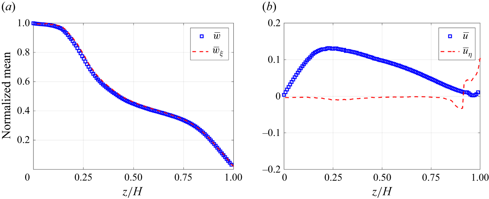
Comparison of mean velocity components in the Cartesian and stream coordinate system for fountain in LSA with
 $\textit{Fr}_0 = 28.2$
.

The importance of employing stream coordinate system is illustrated in figure 9 using the case LSA28N which shows the normalized velocities along the inclined centreline. All the quantities presented are made dimensionless using the source velocity
 $w_0$
. From figure 9(a), it can be observed that no significant discrepancy arises between the mean vertical velocity (
 $\overline {w}$
) and the streamwise component,
 $\overline {w}_{_\xi }$
, along the fountain trajectory. This can be explained upon consideration of (3.11) and noting that the maximum fountain inclination in this case is approximately
 $12^\circ$
. In addition,
 $|\overline {u}| \ll |\overline {w}|$
which results in small values of
 $|\overline {w} - \overline {w}_{_\xi }|$
. Whereas, the mean horizontal velocity (
 $\overline {u}$
) differs considerably from the stream-normal component,
 $\overline {u}_{\eta }$
, as evident from figure 9(b). We see a non-zero contribution in the Cartesian system, an anomaly due to the tilt associated with the fountain. Along the centreline, the normal component of the velocity shall be zero (Khayrullina et al. Reference Khayrullina, van Hooff, Blocken and van Heijst2017). This is captured satisfactorily by the transformed component,
 $u_{_\eta }$
. Therefore, any analysis conducted in the Cartesian system for
 $\overline {\theta } \neq$
0 will be prone to large errors. In the subsequent discussion, we present the velocity statistics of impinging fountains and investigate the influence of lateral density stratification.
Figure 10 presents a direct comparison of the normalized mean centreline velocity for impinging fountains in a UA (filled symbols) with a LSA (open symbols). Figures 10(a) and 10(b) show consistent trends from the LES simulations and experiments, respectively. To facilitate a clear comparison of the decay profiles across different source conditions, the data pairs for each
 $\textit{Fr}_0$
are shifted vertically by an increment of 0.25. Minor differences were observed upon using the distance along the streamline,
 $\xi$
, instead of
 $z$
to plot the data. For every matched set of source conditions, the centreline velocity of the LSA fountains is systematically lower than their UA counterpart. The UA profiles for each
 $\textit{Fr}_0$
serve as a baseline, representing the velocity decay caused by the opposing vertical buoyancy and the adverse pressure gradient upon impingement. The consistent downward shift of the LSA profiles is therefore a direct measure of the additional velocity deficit induced by the lateral stratification.
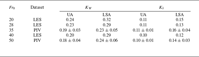
Variation of decay rate of centreline velocity
 $K_W$
, and the spread rate of fountains
 $K_\delta$
as a function of source Froude number obtained from the present simulations (LES) and experiments (PIV).

Dimensionless mean centreline velocity as a function of non-dimensionless vertical distance from (a) LES simulations and (b) PIV measurements. Here UA (filled symbols), LSA (open symbols). Profiles for different source
 $\textit{Fr}_0$
are shifted vertically by 0.25 in an incremental manner for clarity in both panels. This shift is with respect to the bottom most (blue) set of profiles.

To characterize the overall decay of the fountain centreline velocity, we adopt the correlation
 $ ( {w_0}/{\overline {w}_{\xi , cl}} )^{2} = K_W (( {z}/{b_0}) + C_W )$
that is generally used in the context of jets. Here,
 $K_W$
denotes the decay rate and forms one of the metrics widely reported in the literature of free shear flows (Rajaratnam Reference Rajaratnam1976; List Reference List1982). The values of
 $K_W$
were obtained using a curve-fit in region
 $z/H \in$
(0.3, 0.7) and are presented in table 4. This data reveals two important physical trends. First, for both UA and LSA fountains, the decay rate
 $K_W$
decreases with increasing source Froude number. This is physically consistent, as a higher
 $\textit{Fr}_0$
signifies an inertia-dominated flow that can better resist the opposing buoyancy. More importantly, table 4 depicts clearly that
 $(K_W)_{_{\textit{LSA}}} \gt (K_W)_{_{\textit{UA}}}$
for similar source conditions. This higher decay rate in the LSA cases provides a quantitative measure of the additional momentum dissipation caused by the lateral stratification. In the UA, the fountain entrains relatively quiescent fluid. Whereas in the stratified ambient, the fountain entrains fluid that is also subjected to a persistent lateral hydrostatic pressure gradient which is not present in the UA case. This enhanced entrainment-driven mixing, which is later quantified in § 3.3, is the physical mechanism responsible for the more rapid decay of the centreline velocity of fountains in LSA. Therefore, in engineering application such as air curtains or underwater bubble screens, additional energy would need to be expended to counteract the influence of lateral density difference.
3.2.3. Cross-stream statistics
The analysis in the cross-stream direction is carried out along
 $x_\eta$
instead of the Cartesian
 $x$
as highlighted in § 3.2.2. The difference between the two scenarios can be appreciated further upon consideration of the impinging fountain in a LSA (case LSA28N:
 $\textit{Fr}_0 = 28.2$
,
 $D_m = 0.4$
). Figure 11(a) shows the spatial distribution of dimensionless mean velocity magnitude. Corresponding to different values of
 $z/H$
shown by the magenta lines, the spatial locations of peak velocity magnitude are shown by green squares. According to local
 $\overline {\theta } (z)$
, we obtain the stream-normal direction as indicated by the blue lines along which further investigation is conducted. This form of analysis has previously been adopted by researchers for curved jets and fountains (Ramaprian & Haniu Reference Ramaprian and Haniu1989; Mahesh Reference Mahesh2013). Turbulent fountains entrain ambient fluid and grow laterally as a result. This spread is often quantified using the changes in the half-width (
 $\delta$
) which is defined as the distance from the fountain axis along
 $x_\eta$
at which the streamwise velocity reduces to half of its centreline value. In figure 11(a), these locations are marked using red and black circles on the buoyant (
 $\delta _B$
) and non-buoyant (
 $\delta _{\textit{NB}}$
) sides, respectively.
(a) Spatial distribution of normalized mean velocity. Magenta lines represent the horizontal (
 $x$
) cross-sections, whereas blue lines show stream-normal (
 $x_\eta$
) directions. Circles and triangles represent the half-width and locations corresponding to twice the half-width, respectively. (b) Variation of dimensionless average half-width from experiments (
 $\textit{Fr}_0 \approx 35$
) and numerical simulations (
 $\textit{Fr}_0 = 28.2$
) for fountains in UA and LSA.

Figure 11(b) shows the variation of the normalized average half-width,
 $\delta = (\delta _B +{} \delta _{\textit{NB}})/{2 b_0}$
for a particular source condition, obtained from the LES data and compared with the corresponding PIV estimates. A reasonably good agreement is observed between the two datasets. The rate of spread (
 $\propto {{\rm d} \delta }/{{\rm d}z}$
) of fountains in LSA is distinguishably larger than their UA counterparts. This suggests higher fluid entrainment in LSA cases which is driven by the lateral hydrostatic pressure gradients. The spreading rate (
 $K_\delta$
) for all the cases is formally quantified using the correlation
 ${\delta }/{b_0} = K_\delta (( {z}/{b_0}) + C_\delta )$
and is presented in table 4. The estimates of
 $K_\delta$
are consistently larger in LSA for the range of Froude number considered in experiments and simulations. This highlights that an ambient stratification affects the horizontal growth of the fountains. As
 $\textit{Fr}_0$
increases, this lateral spreading is reduced with the flow resembling a canonical jet once
 $\textit{Fr}_0 \rightarrow \infty$
. The value of
 $K_\delta$
for this case was calculated as 0.1 (not shown here) from LES and PIV. We use the ratio of the half-widths on the buoyant and non-buoyant sides,
 $r_{_\delta } = \delta _B/\delta _{\textit{NB}}$
, to examine the asymmetry in lateral development of the fountain. Here
 $r_{_\delta }$
allows for the separation of the contribution of buoyant and non-buoyant fluid entrained into the core of the turbulent fountain. Figure 12(a) presents the estimates of
 $r_{_\delta }$
as a function of the source Froude number. The symmetrical ambient of the UA cases results in
 $r_{_\delta } \approx 1$
as the fountain expands equally on both sides. As a lateral stratification is imposed, the fountain entrains fluid asymmetrically. Here
 $r_{_\delta } \gt 1$
implies that the fountains are slightly stretched on the buoyant side. The structural asymmetrical characteristics, that were discussed in § 3.1.2, thus leads to an asymmetric fountain spread.
(a) Ratio of half-width,
 $r_{_\delta } = \delta _B/\delta _{\textit{NB}}$
, as a function of
 $\textit{Fr}_0$
for fountains in UA (filled symbols) and LSA (open symbols). (b) Dimensionless mean streamwise velocity plotted against normalized cross-stream distance. The X-axis is made non-dimensional using
 $\delta _B$
and
 $\delta _{\textit{NB}}$
on the positive and negative sides, respectively.

We now examine if the initial asymmetry in the LSA cases is also manifested in the shape of the mean velocity profile. This is a critical question from both a physical and a modelling perspective. Figure 12(b) shows the mean streamwise velocity, normalized by the local centreline value, plotted against the cross-stream distance. Crucially, the cross-stream distance has been normalized independently on the buoyant (
 $\delta _B$
) and non-buoyant (
 $\delta _{\textit{NB}}$
) sides by the respective local half-widths. For both UA and LSA cases from experiments and simulations, a single Gaussian profile was observed to fit the data very well. This clear collapse was not observed if the average half-width
 $\delta$
was used for normalization making this finding non-trivial. While a Gaussian shape is typical for canonical jets and fountains in an unstratified ambient, its recovery from a fundamentally asymmetric flow, is only possible due to this asymmetric normalization. Therefore, the lateral stratification in the system asymmetrically alters the characteristic length scale of the fountain. Although not shown here, the mean velocity distribution remains self-similar across different values of
 $z/H \in [0.25, 0.75]$
.
Estimates of normalized (a) r.m.s. streamwise velocity and (b) r.m.s. stream-normal velocity obtained from experiments and simulations. The normalization of the X-axis is similar to figure 12.

Quantitative analysis of the fountain’s lateral flapping motion at
 $z/H = 0.5$
. (a) Range of dimensionless centreline deflection at fountain midheight comparing fountains in UA with that in LSA. (b) The PSD of the experimental centreline position against Strouhal number.

Figure 13 shows the corresponding variation of root-mean-square (r.m.s.) velocity statistics computed from the LES data and PIV measurements for the chosen case. The streamwise velocity fluctuations plotted in figure 13(a) compare the fountains in UA with their laterally stratified counterpart. The numerical data suggests a slight reduction in the peak value of
 $\sqrt {w_\xi ^\prime w_\xi ^\prime }$
which is more substantiated on the buoyant side (
 $x_\eta \gt x_{cl}$
). This represents a larger damping of the turbulent fluctuations by the dense ambient fluid on the buoyant side, as compared with the non-buoyant half where the source fluid interacts with fluid of essentially similar density. Interestingly, the experimental data does not show this asymmetry, but rather an amplification of streamwise fluctuations across the entire profile compared with the UA case. The cause of this discrepancy is revealed by a quantitative analysis of the fountain’s lateral flapping motion at
 $z/H = 0.5$
, presented in figure 14. Figure 14(a) plots the mean centreline location and the corresponding standard deviation which is a direct measure of the flapping amplitude. The data clearly indicates that this amplitude is noticeably larger in LSA experiments as compared with the numerical data, and the fountains in UA. This provides quantitative evidence that the larger-scale unsteadiness in the experiments results in the smearing of asymmetry which is observed in our numerical datasets. To further characterize the nature of this motion, a spectral analysis of the experimental centreline position is presented in figure 14(b). The power spectral density (PSD) for both UA and LSA cases indicate that the energy is concentrated at low Strouhal numbers (
 $St = fb_0/w_0 \lt 0.02$
). More importantly, the spectral energy content for LSA case is nearly an order of magnitude greater than for the UA case, which depicts the role of lateral density stratification towards energizing the low-frequency flapping mode of the fountain.
The corresponding r.m.s. statistics of the cross-stream velocity component (
 $u_\eta ^\prime$
) are shown in figure 13(b). The numerical and experimental estimates point towards increased stream-normal fluctuations in the LSA cases as compared with the UA fountain. This shows that the lateral stratification induces a strong anisotropy in the turbulence profiles. It damps fluctuations in the primary direction of motion while amplifying the cross-stream fluctuations that are most effective at driving entrainment of the ambient fluid.
Variation of dimensionless (a) volume flux and (b) momentum flux along the centreline of fountains in UA and LSA. Quantities have been normalized with their respective source values.

3.3. Quantification of turbulent entrainment
The previous sections discussed the effects of lateral density stratification on the structural and statistical characteristics of impinging line fountains. We will now compute integral fluxes from these statistics and estimate the entrainment coefficient
 $\alpha$
. We first estimate the volume and momentum fluxes per unit length of the fountain source as
 \begin{align} Q = \int _{- \infty }^{\infty } \overline {w}_{_\xi } \ {\rm d} x_{_\eta } \approx \int _{- 2\delta _{_{\textit{NB}}}}^{2\delta _{_B}} \overline {w}_{_\xi } \ {\rm d} x_{_\eta }, \\[-12pt]\nonumber \end{align}
 \begin{align} M = \int _{- \infty }^{\infty } \overline {w}_{_\xi }^2 \ {\rm d} x_{_\eta } \approx \int _{- 2\delta _{_{\textit{NB}}}}^{2\delta _{_B}} \overline {w}_{_\xi }^2 \ {\rm d} x_{_\eta }. \end{align}
The integration limits in (3.13) have been chosen as twice the respective half-width locations, with the justification for this selection provided in S1 in the Supplementary material is available at https://doi.org/10.1017/jfm.2026.11318. Figure 15(a) shows the variation of the normalized volume flux,
 $Q/Q_0$
, along the axis of the fountains. For all cases,
 $Q$
increases monotonically up to
 $z/H \approx$
0.7, indicating net entrainment of the ambient fluid. In the near-wall region beyond this point, the volume flux decreases (see numerical datasets), signifying fluid detrainment as the impinging fountain is forced along diverging streamlines. The main finding from this data is that for similar source conditions (
 $Q_0, \textit{Fr}_0$
), the lateral stratification leads to a consistently and noticeably higher volume flux in the fountain, a trend observed in both the experimental and numerical data. This result is significant as it provides the integral evidence for the enhanced lateral growth discussed in the preceding sections. The corresponding variation of normalized momentum flux,
 $M/M_0$
, is shown in figure 15(b). The UA case serves as a baseline for which the momentum flux is approximately conserved, i.e.
 $M \approx 0.9M_0$
in the self-similar region. The subsequent sharp decay is a consequence of the deceleration induced by the adverse pressure gradients at the impingement surface. On the other hand, fountains in a LSA are not momentum-conserving. They exhibit a systematic decay along their axis and the integral momentum flux remain lower than their UA counterparts. This momentum deficit is primarily due to the higher entrainment as the fountain expend its initial momentum to accelerate the larger volume of entrained, slow-moving ambient fluid. This confirms that the lateral stratification introduces an additional mechanism for momentum dissipation, which leads to higher values of
 $K_W$
obtained previously.
The entrainment coefficient
 $\alpha$
is now calculated using the framework formulated by Morton, Taylor & Turner (Reference Morton, Taylor and Turner1956). For incompressible planar flows assuming two-dimensionality, the mean continuity equation integrated and after an algebraic rearrangement yields (Parker et al. Reference Parker, Burridge, Partridge and Linden2020)
 \begin{equation} \frac {{\rm d}Q}{{\rm d}z} = 2 \alpha \frac {M}{Q}. \end{equation}
Here,
 $\alpha$
is notionally equivalent to the ratio of the entrainment velocity at the edge of the fountain to the corresponding centreline velocity, i.e.
 \begin{equation} \alpha = \frac {\displaystyle {\lim _{x \to \infty }} |\overline {u}_\eta |}{\overline {w}_{\xi , {cl}}}. \end{equation}
Thus, an integral estimate of
 $\alpha$
can be obtained from (3.14) as
 \begin{equation} \alpha = \frac {Q}{2M} \frac {{\rm d}Q}{{\rm d}z}. \end{equation}
Integral entrainment coefficient calculated from (a) LES simulations and (b) PIV measurements. Here UA (filled symbols), LSA (open symbols). Profiles for different source
 $\textit{Fr}_0$
are shifted vertically for clarity in both panels.

Figure 16 compares the estimates of integral entrainment coefficient for fountains in UA with those in LSA, with consistent trends observed between the LES simulations (figure 16
a) and the PIV measurements (figure 16
b). Profiles for different source
 $\textit{Fr}_0$
are shifted vertically for clarity. The profiles for all cases exhibit a characteristic shape where
 $\alpha$
increases from zero at the source to a peak value near the fountain’s midheight (
 $z/H \approx 0.5$
). Beyond this point,
 $\alpha$
decreases and eventually becomes negative in the near-wall region. The initial increase corresponds to the region of strong entrainment where the volume flux
 $Q$
grows rapidly, while the negative values near the wall signify detrainment as the flow is forced along diverging streamlines by the impingement surface. Experimental values of entrainment coefficient were not possible near the wall due to limited field of view. The primary finding of this analysis is the significant increase in the entrainment coefficient for the LSA cases, which is up to 20 % higher than in the corresponding UA cases. This is the direct quantification of the enhanced mixing between the fountain and ambient fluids hypothesized in the previous sections. This enhanced entrainment is the underlying mechanism responsible for all the previously observed macroscopic effects including the faster centreline velocity decay (
 $K_W$
), the larger spreading rates (
 $K_\delta$
) and the higher volume flux. In the context of practical utility, for instance, when it is desirable to maintain a building space at specific conditions, e.g. temperature, humidity, etc., the enhanced entrainment in air curtains may put additional load on the heating, ventilation and air-conditioning system. In underwater bubble screens, this may manifest as higher salt concentration in a freshwater ambient, which could demand desalination if these levels become too high.
4. Conclusions
This study presented a systematic investigation of turbulent line fountains discharged into a LSA, using a synergistic approach of high-resolution LES computations and refractive-index matched PIV experiments. The spatiotemporal evolution, velocity statistics and entrainment characteristics were compared with fountains in a UA. We have shown that the deflection modulus,
 $D_m$
, largely governs the flow regime. For low
 $D_m$
, the lateral stratification results in a complete sideway deflection, while for higher
 $D_m$
, the fountain possesses sufficient momentum to impinge, forming an asymmetric pair of buoyant and non-buoyant wall jets. For the UA case, a new analytical model for the lateral spread of the buoyant wall jet was developed and validated against the LES data. It was shown that this lateral spread scaled as
 $\textit{Fr}_0^{5/4}$
. The studied configuration inherently imposes a bidirectional, gravity-driven cross-flow. Under the action of this cross-flow, the trajectory of the LSA fountains was computed for a wide range of
 $D_m$
and was shown to follow a universal scaling law. As demonstrated in figure 8(b), the scaled trajectory collapses onto a power law with an exponent of
 $p = 4$
, leading to the dimensional scaling
 $x_{cl} \propto {z^2}/{\textit{HD}_m}$
. This exponent is significantly steeper than the
 $p = 3$
exponent for a line jet in a unidirectional cross-flow, a finding that points to a distinct physical mechanism. The impingement induces an adverse pressure gradient for high
 $D_m$
fountains, whereas for deflecting fountains, the counter-propagating gravity currents exert a bidirectional lateral force to steepen the fountain trajectory.
A central contribution of this work is the detailed characterization of the velocity statistics, which revealed several new physical insights into the behaviour of fountains in a LSA. We have shown that the lateral stratification leads to a more rapid decay of the mean streamwise velocity compared with the UA case. This is a direct consequence of enhanced entrainment, as confirmed by the higher lateral spreading rates observed in the LSA fountains. More importantly, this enhanced mixing is fundamentally asymmetric. The fountain’s spread was consistently found to be markedly greater on the buoyant side from LES and PIV datasets. This asymmetry in the mean flow is a macroscopic manifestation of an underlying anisotropy in the turbulence structure. Our numerical simulations revealed that while the streamwise r.m.s. velocity fluctuations are damped on the buoyant side due to opposing buoyancy, the stream-normal fluctuations, which are the primary drivers of entrainment, are simultaneously amplified. Finally, the synergistic use of experiments and simulations was essential for understanding the fountain’s unsteadiness. While the LES data cleanly isolated the local, asymmetric turbulence, the experimental r.m.s. profiles showed a general amplification of fluctuations without this clear asymmetry. This discrepancy was quantitatively explained by a spectral analysis of the fountain’s centreline motion, which showed that the lateral stratification may have actively energized the natural, low-frequency flapping mode. The significantly larger flapping amplitudes in the experiments were responsible for the smoothening of the time-averaged asymmetry.
The integral entrainment coefficient
 $\alpha$
provides the most fundamental measure of the mixing dynamics. The quantification of
 $\alpha$
presented in figure 16, completes the physical argument. The data confirms that the entrainment coefficient is consistently and significantly higher by up to 20 % for the LSA cases compared with their UA counterparts. This result provides an integral validation for the enhanced fluid ingress discussed throughout this study. The higher value of
 $\alpha$
is the direct macroscopic consequence of the stronger forcing at the fountain’s boundary, which is induced by the interaction of the fountain’s entrainment demand with the persistent lateral pressure field. Ultimately, this enhanced entrainment is the underlying physical driver for all the previously observed phenomena in the LSA cases including the faster centreline velocity decay (
 $K_W$
), the larger spreading rates (
 $K_\delta$
) and the higher volume flux. The quantification of
 $\alpha$
thus unifies our findings into a single, self-consistent physical picture.
Supplementary material
Supplementary material is available at https://doi.org/10.1017/jfm.2026.11318.
Acknowledgements
We would like to extend our sincere thanks to the technical staff of the fluid mechanics laboratory, as well as to A. Kaur and S. Mittal for their invaluable help during the experiments. We also deeply appreciate the insightful discussions with Dr E. Santilli from Thomas Jefferson University, whose guidance on setting up the LES simulations using SOMAR significantly contributed to the present research. We also thank three anonymous referees for their insightful comments and constructive criticism, which significantly improved the structure and the focus of this paper. T.A. acknowledges the assistance provided by A. Gandhi for creating the schematics, and to S. Srivastava and S. Narayan Dhar for proofreading the manuscripts. The authors thank IIT Delhi HPC facility for computational resources.
Funding
T.A. expresses gratitude for the Prime Minister Research Fellowship (PMRF) awarded by the Government of India, while N.K.J. acknowledges the seed grant (PLN12/04AM) and matching grant (MI02572G) supports from the Indian Institute of Technology Delhi.
Declaration of interests
The authors have no competing interests to declare that are relevant to the content of this article.
Data availability statement
The data that support the findings of this study are available from the corresponding author upon reasonable request.
Appendix A. Computational grid
A two-level nested grid is employed in the present simulations where the base mesh contains 1024
 $\times$
64
 $\times$
128 points which covered the entire flow domain. This mesh was established after a carefully performed grid-independence study reported previously by Agrawal et al. (Reference Agrawal, Jha and Chalamalla2023b
). A finer level was overlaid in the central region of the computational domain to accurately capture the small-scale features developing in the high shear region in the vicinity of the fountain. The spatial extent of this mesh in the
 $x$
-direction ranged between
 $( {x}/{b_0} )\in$
(−7, 8.7), whereas it covered the entire vertical and spanwise region. The slight bias in the positive
 $x$
-direction is provided to consider the effect of lateral deflection as shown later. Essentially, the finer grid comprised of 432
 $\times$
128
 $\times$
512 points resulting in a spatial resolution of approximately
 $\Delta x \times \Delta y \times \Delta z \equiv ( {b_0}/{28} )\times ( {b_0}/{6}) \times ({b_0}/{12})$
. On the finer level, we obtain an average value of
 ${{\rm d}l} \approx 6\eta$
, indicating a well-resolved LES. Here,
 ${\rm d}l = \sqrt [3]{\Delta x \Delta y \Delta z}$
, and
 $\eta = ({\nu ^3}/{\epsilon } )^{1/4}$
represents the Kolmogorov microscale (Davidson Reference Davidson2015). Here
 $\epsilon$
is the dissipation rate of turbulent kinetic energy and is calculated as
 $(\nu + \nu _{\textit{sgs}}) s_{\textit{ij}} s_{\textit{ij}}$
where
 $s_{\textit{ij}}$
denotes the strain rate associated with the fluctuating velocity field. For the most energetic case (
 $\textit{Fr}_0 = 40.1$
), the average value of
 ${{\rm d}l}/{\eta } \approx$
6, indicates a well-resolved LES on the finer level that surrounds the core of the impinging fountain.
Appendix B. Refractive index matching
For the optical investigation carried out in the present study, it is essential to match the refractive index,
 $n$
, of the participating fluids to avoid anomalies in the PIV images. Towards this, we use the combination of aqueous solutions of NaCl and NaNO
 $_3$
, previously employed by Olsthoorn & Dalziel (Reference Olsthoorn and Dalziel2017) among others, in their study concerning stratified fluids. Figure 17 shows the measured density and refractive index of these salt solutions. Therefore, matching the refractive index yields an aqueous solution of sodium nitrate that has a higher density than the aqueous NaCl, and thus, has been used as the denser fluid in the system having density
 $\rho _d$
. On the other hand, the supply fluid as well as the lighter half of the tank is obtained by dissolving sodium chloride.
Density as a function of refractive index for the aqueous solutions of salts used for experiments.

Appendix C. Experimental details
The experiment commences with turning on the supply pump, and the resulting flow is given some time to establish which is usually approximately
 $t_0 =$
10 s, after which the flow rate through the turbine flow meter is constant. During this period, aqueous sodium nitrate solution is simultaneously added to the other side of the tank to ensure same fluid levels across the LG. Once the flow establishes, the LG is rapidly released to allow interaction of the line fountain with the lateral buoyancy field. The gate is kept opened for
 $t_{ex} \approx$
60 s during which the fluid exchange occurs between reservoirs of density
 $\rho _l$
and
 $\rho _d$
. Optical probing is conducted in the central region to quantify the velocity dynamics of the fountains. After image acquisition, the LG is subsequently reinstalled securely followed by turning off the supply pump. The valve V2 is also kept shut hereon to prevent any potential reverse flow caused by gravity-induced siphoning.
For PIV measurements, polyamide particles of diameter
 $\phi _s =$
60 μm (LaVision), are mixed in the experimental tank as well as the supply tank, ST. These particles are illuminated using a 5 W continuous-wave laser (
 $\lambda =$
532 nm; Changchun New Industries) in a streamwise–lateral (
 $z$
–
 $x$
) plane, placed approximately in the centre in spanwise (
 $y$
) direction. We use cylindrical optics to create a laser sheet of nominal thickness 2 mm. A high-speed camera (Photron FASTCAM MINI UX 100), mounted with a 100 mm F/2.8 lens, is used to record the image sequence at 500 Hz with a resolution of 1024
 $\times$
1024 pixels. The field-of-view of the camera encompasses the region between
 $z/H \approx$
0.25 to
 $z/H \approx$
0.75, where
 $z$
is measured from the nozzle exit. In present measurements, we do not acquire images throughout the time period of
 $t_{ex}$
seconds due to memory constraints inherent to the high-speed camera. Instead, the recording begins approximately 15 s after the removal of the LG to eliminate any disturbance that might have been caused due to sudden removal of the gate, and also to let the line fountain establish. The total recording time in our experiments is limited to
 $t_{aq} \approx$
21.8 s, equivalent to approximately 10 900 snapshots, that was deemed sufficient to obtain the converged statistics. We use the PIVlab suite developed by Thielicke & Sonntag (Reference Thielicke and Sonntag2021) to process the raw images to obtain the instantaneous velocity fields. A multigrid algorithm is used that employs three successive passes to yield the resultant velocity field over windows of size 24
 $\times$
24 pixels, thereby providing an effective spatial resolution of 1.4 mm.
(a) Temporal evolution of normalized velocity at the central point of the domain. (b) Short-time averaged fountain centreline.

Appendix D. Spatiotemporal averaging
The fountains evolve from a quiescent phase to a quasisteady state. Statistics presented in § 3.2 were estimated using (3.7). We choose the case LSA28N to demonstrate the temporal aspect of this double-averaging process. Consideration of the point
 $(x_{cl} (L/2), W/2, H/2)$
that lies on the axis of the fountain and in the centre planes, provides insight into the pointwise development of velocity field in the inner core. The variation of normalized velocity at this point is shown in figure 18(a). Data points in time windows corresponding to every two flow-through times (2
 $T_{\!f} =$
2
 $H/w_0$
) are coloured differently and their short-time window average is shown using the horizontal black lines. It can be seen that beyond 2
 $T_{\!f}$
, the average values are relatively consistent and are found to be within 15 % of their neighbouring averages. However, if the corresponding short-time averaged fountain centreline is inspected, the convergence is achieved much later as shown in figure 18(b). We note that the fountain centreline exhibits a transient variation up to approximately 8
 $T_{\!f}$
. Solid red line in the figure shows the long time-averaged centreline evaluated over the total averaging interval. In the analysis presented in this paper, the time instant at which the averaging begins has been chosen as the maximum of these two estimates.