2.1. Governing equations

The governing equations for the EAS-DDES model (Liu et al. Reference Liu, Zhang, Yin and He2024b) read as

(2.1) \begin{align} \begin{aligned} \boldsymbol{\nabla } \boldsymbol{\cdot }\boldsymbol{ \bar {u}} &= 0, \\ \frac {{D} \boldsymbol{ \bar {u}}}{{D} t} &= -\boldsymbol{\nabla \!} \bar {p} + \boldsymbol{\nabla } \boldsymbol{\cdot }\left ( \nu \boldsymbol{\nabla } \bar {u}\right ) - \boldsymbol{\nabla } \boldsymbol{\cdot }\boldsymbol{\tau }, \\ \frac {{D} k}{{D} t} &= - \boldsymbol{\tau } : \boldsymbol{\bar {S}} -C_\mu k \omega +\boldsymbol{\nabla } \boldsymbol{\cdot }\left [ \left (\nu + \frac {C_\mu ^* \sigma _k}{C_\mu } \frac {k}{\omega } \right ) \boldsymbol{\nabla } k\right ]\!, \\ \frac {{D} \omega }{{D} t} &= \frac {2C_{\omega 1}C_\mu ^*}{C_\mu } |\bar {S}|^2 - C_{\omega 1}\omega \boldsymbol{a^*} : \boldsymbol{\bar {S}} - C_{\omega 2} \omega ^2+\boldsymbol{\nabla } \boldsymbol{\cdot }\left [ \left (\nu + \frac {C_\mu ^* \sigma _\omega }{C_\mu } \frac {k}{\omega } \right ) \boldsymbol{\nabla } \omega \right ]\!, \end{aligned} \end{align}

where $p$ denotes the pressure normalized by the constant flow density, $\boldsymbol{u}$ is the velocity, $\nu$ is the kinetic viscosity, $k$ is the TKE, $\omega$ is the turbulence frequency, $C_\mu$ is the standard eddy viscosity coefficient, $C_\mu ^*$ represents the effective $C_\mu$ and $\boldsymbol{\bar {S}}$ denotes the strain rate tensor as

(2.2) \begin{equation} \boldsymbol{\bar {S}} \equiv \dfrac {1}{2} \big [ \boldsymbol{\nabla }\boldsymbol{ \bar {u}} + (\boldsymbol{\nabla } \boldsymbol{ \bar {u}})^{{T}} \big]. \end{equation}

Here, the RANS ensemble-average and the LES spatial-filtering are collectively denoted by the overline $\bar {(\boldsymbol{\cdot })}$ . The standard values of the model constants are adopted as $C_\mu = 0.09$ , $\sigma _k = \sigma _\omega = 0.5$ , $C_{\omega 1} = 5/9$ , $C_{\omega 2} = 3/40$ .

The modelled stress $\boldsymbol{\tau }$ is expressed as (Liu et al. Reference Liu, Zhang, Yin and He2024b)

(2.3) \begin{equation} \boldsymbol{\tau } \equiv \overline {\boldsymbol{uu}} - \bar {\boldsymbol{u}} \bar {\boldsymbol{u}} = k \boldsymbol{a} + \dfrac {2}{3}k \boldsymbol{I} = -2\nu _t \boldsymbol{\bar {S}} + k \boldsymbol{a^*} + \dfrac {2}{3}k \boldsymbol{I}. \end{equation}

In the EAS-DDES model, the linear part $(-2\nu _t\bar {S})$ directly controls the switching between the RANS and LES branches through the eddy viscosity $\nu _t$ , and the nonlinear part $\boldsymbol{a^*}$ reacts to that, adding the extra anisotropy to the modelled stress. In the following, the modelling of the linear and nonlinear parts of the turbulent stress is illustrated, respectively.

2.2. Modelling of the linear part in the DDES manner

The linear part of the turbulent stress is modelled by following the $\ell ^2-\omega$ DDES framework (Reddy et al. Reference Reddy, Ryon and Durbin2014). Specifically, the eddy viscosity $\nu _t$ in the linear part is calculated as

(2.4) \begin{equation} \nu _t = \ell _{\textit{DDES}}^2 \omega . \end{equation}

The DDES length scale $\ell _{\textit{DDES}}$ calculated from the RANS and LES length scales ( $\ell _{\textit{RANS}}$ and $\ell _{\textit{LES}}$ ) as

(2.5) \begin{equation} \ell _{\textit{DDES}} = \ell _{\textit{RANS}} - f_d \max (0, \ell _{\textit{RANS}} - \ell _{\textit{LES}}), \end{equation}

where

(2.6) \begin{equation} \begin{aligned} \ell _{\textit{RANS}} &= \sqrt {\frac {C_\mu ^*}{C_\mu }} \frac {\sqrt {k}}{\omega }, \quad \ell _{\textit{LES}} = C_{\textit{DES}} \varDelta ,\\ \varDelta &=f_d V^{1 / 3}+\left (1-f_d\right ) h_{max } . \end{aligned} \end{equation}

Here $V$ is the local cell volume, and $h_{max}$ is the local maximum cell spacing in the three directions. The shielding function $f_d$ is to ensure the near-wall RANS region, which is formulated as

(2.7) \begin{equation} f_d = 1 - \tanh [(8r_d)^3], \quad r_d = \frac {(C_\mu ^*/ C_\mu )k/\omega + \nu }{\kappa ^2 d_w^2 \sqrt {\boldsymbol{\nabla }\boldsymbol{ \bar {u}} : \boldsymbol{\nabla }\boldsymbol{ \bar {u}}}} \end{equation}

with $\kappa$ being the von Kármán constant, and $d_w$ the wall distance.

2.3. General expression of the nonlinear part

As for the nonlinear extra anisotropy $\boldsymbol a^*$ , the most general expression is adopted as (Pope Reference Pope1975)

(2.8) \begin{equation} \boldsymbol{a^*} = \sum _{i=2}^{10} \beta _i \boldsymbol{T}_i, \end{equation}

which is derived under the effective-viscosity hypothesis and the Cayley–Hamilton theorem. Here $\boldsymbol{T}_i$ are the tensor basis as

(2.9) \begin{equation} \begin{aligned} &\boldsymbol{T}_2 = \boldsymbol{S}^2 - \dfrac {1}{3} \theta _1 \boldsymbol{I} , \quad \boldsymbol{T}_3 = \boldsymbol{\varOmega }^2 - \dfrac {1}{3} \theta _2 \boldsymbol{I} , \quad \boldsymbol{T}_4 = \boldsymbol{S}\boldsymbol{\varOmega } - \boldsymbol{\varOmega }\boldsymbol{S} , \\ &\boldsymbol{T}_5 = \boldsymbol{S}^2\boldsymbol{\varOmega } - \boldsymbol{\varOmega }\boldsymbol{S}^2 , \quad \boldsymbol{T}_6 = \boldsymbol{S}\boldsymbol{\varOmega }^2 + \boldsymbol{\varOmega }^2\boldsymbol{S} - \dfrac {2}{3} \theta _4 \boldsymbol{I} - \theta _2 \boldsymbol{S}, \\ & \boldsymbol{T}_7 = \boldsymbol{S}^2\boldsymbol{\varOmega }^2 + \boldsymbol{\varOmega }^2\boldsymbol{S}^2 - \dfrac {2}{3} \theta _5 \boldsymbol{I} - \theta _4 \boldsymbol{S} , \quad \boldsymbol{T}_8 = \boldsymbol{S}\boldsymbol{\varOmega }\boldsymbol{S}^2 - \boldsymbol{S}^2\boldsymbol{\varOmega }\boldsymbol{S}, \\ & \boldsymbol{T}_9 = \boldsymbol{\varOmega }\boldsymbol{S}\boldsymbol{\varOmega }^2 - \boldsymbol{\varOmega }^2\boldsymbol{S}\boldsymbol{\varOmega } , \quad \boldsymbol{T}_{10} = \boldsymbol{\varOmega }\boldsymbol{S}^2\boldsymbol{\varOmega }^2 - \boldsymbol{\varOmega }^2\boldsymbol{S}^2\boldsymbol{\varOmega } , \end{aligned} \end{equation}

with $\boldsymbol I$ being the identity matrix. The tensor coefficients $\beta _i$ depend on the five invariants as

(2.10) \begin{equation} \theta _1 = \textrm {tr} (\boldsymbol{S}^2), \quad \theta _2 = \textrm {tr} (\boldsymbol{\varOmega }^2) , \quad \theta _3 = \textrm {tr} ( \boldsymbol{S}^3 ) , \quad \theta _4 = \textrm {tr} ( \boldsymbol{S \varOmega }^2 ) , \quad \theta _5 = \textrm {tr} ( \boldsymbol{S}^2 \boldsymbol{\varOmega }^2 ) . \end{equation}

The normalized strain and rotation rates are defined as

(2.11) \begin{equation} \boldsymbol{S} \equiv \frac {\boldsymbol{\nabla }\boldsymbol{ \bar {u}} + (\boldsymbol{\nabla } \boldsymbol{ \bar {u}})^{{T}}}{2C_\mu \omega } , \quad \boldsymbol{\varOmega } \equiv -\frac {\boldsymbol{\nabla } \boldsymbol{\bar {u}} - (\boldsymbol{\nabla } \boldsymbol{\bar {u}})^{{T}}}{2C_\mu \omega } . \end{equation}

Note that the tensor bases $\boldsymbol{T}_6$ and $\boldsymbol{T}_7$ differ from the original expressions of Pope (Reference Pope1975) in the existence of the last terms. This is due to the extraction of the linear components, which are absorbed into the linear part of the modelled stress. Accordingly, $C_\mu ^*$ is expressed as

(2.12) \begin{equation} C_\mu ^{*} = -\dfrac {1}{2}(\beta _1 + \theta _2\beta _6 + \theta _4 \beta _7) \end{equation}

where $\beta _1$ represents the coefficient of the first tensor basis $\boldsymbol{T}_1 = \boldsymbol{S}$ in the general expression of $\boldsymbol{a}$ .

2.4. Closure through the algebraic stress equation

To close the tensor basis coefficients $\beta _i$ , the algebraic stress modelling framework is adopted under the weak-equilibrium assumption. The transport of the modelled stress $\boldsymbol{\tau }$ can be considered to be due to transports in $k$ and modelled stress anisotropy $\boldsymbol{a}$ . The former is retained, while the latter is neglected (Pope Reference Pope2000), resulting in an implicit algebraic equation of $\boldsymbol{a}$ as

(2.13) \begin{equation} \left(\boldsymbol{a} + \dfrac {2}{3}\boldsymbol{I}\right)(\mathcal{P}-\varepsilon )= \boldsymbol{P}-\boldsymbol{E}+\boldsymbol{\varPi } \text{,} \end{equation}

where the production tensor $\boldsymbol{P}$ is in closed form as

(2.14) \begin{equation} \boldsymbol{P} \equiv - \boldsymbol{\tau } \boldsymbol{\nabla }\boldsymbol{ \bar {u}} - (\boldsymbol{\nabla }\boldsymbol{ \bar {u}})^{{T}} \boldsymbol{\tau } = \varepsilon \left(\!-\dfrac {4}{3}\boldsymbol{S} - \boldsymbol{aS} - \boldsymbol{Sa} + \boldsymbol{a \varOmega } - \boldsymbol{\varOmega a}\right)\! , \end{equation}

and $\mathcal{P} \equiv \textrm {tr}(\boldsymbol{P})/2$ . For the dissipation tensor $\boldsymbol{E}$ , lumping the dissipation anisotropy into the pressure–strain rate tensor $\boldsymbol{\varPi }$ results in (Pope Reference Pope2000)

(2.15) \begin{equation} \boldsymbol{E} = \dfrac {2}{3} \varepsilon \boldsymbol{I} . \end{equation}

The pressure–strain rate tensor $\boldsymbol{\varPi }$ can be decomposed into a slow and a rapid component, i.e. $\boldsymbol{\varPi }^s$ and $\boldsymbol{\varPi }^r$ , respectively. The Rotta model (Rotta Reference Rotta1951) is used for $\boldsymbol{\varPi }^s$ as

(2.16) \begin{equation} \boldsymbol{\varPi }^s = -C_1 \varepsilon \boldsymbol{a} , \end{equation}

representing a linear return to isotropy of the Reynolds stress. The Rotta constant $C_1$ determines the rate of return to isotropy. As for the rapid pressure–strain rate $\boldsymbol{\varPi }^r$ , there exist several models (Pope Reference Pope2000). Here we follow Taulbee (Reference Taulbee1992) and Wallin & Johansson (Reference Wallin and Johansson2000) to adopt the general linear model of Launder, Reece & Rodi (Reference Launder, Reece and Rodi1975) for $\boldsymbol{\varPi }^{r}$ as

(2.17) \begin{align} \boldsymbol{\varPi }^{r}=-\frac {C_2+8}{11}\left (\boldsymbol{P}-\frac {2}{3} \mathcal{P} \boldsymbol{I}\right )-\frac {60 C_2-4}{55} \varepsilon \boldsymbol{S}-\frac {8 C_2-2}{11}\left (\boldsymbol{D}-\frac {2}{3} \mathcal{P} \boldsymbol{I}\right )\! , \end{align}

where

(2.18) \begin{equation} \boldsymbol{D} \equiv - \boldsymbol{\tau } (\boldsymbol{\nabla }\boldsymbol{ \bar {u}})^{{T}} - (\boldsymbol{\nabla }\boldsymbol{ \bar {u}}) \boldsymbol{\tau } = \varepsilon\! \left(\!-\dfrac {4}{3}\boldsymbol{S} - \boldsymbol{aS} - \boldsymbol{Sa} - \boldsymbol{a \varOmega } + \boldsymbol{\varOmega a}\right)\! . \end{equation}

Inserting (2.14)–(2.18) into (2.13), the algebraic equation for the modelled stress anisotropy tensor $\boldsymbol{a}$ is derived as

(2.19) \begin{equation} \left (C_1 - 1 + \frac {\mathcal{P}}{\varepsilon } \right ) \boldsymbol{a}=-\frac {8}{15} \boldsymbol{S} +\frac {7C_2 +1}{11}(\boldsymbol{a} \boldsymbol{\varOmega }-\boldsymbol{\varOmega } \boldsymbol{a})-\frac {5-9C_2}{11}\big [\boldsymbol{a S}+\boldsymbol{S a}-\dfrac {2}{3} \operatorname {tr} (\boldsymbol{a} \boldsymbol{S}) \boldsymbol{I} \big ] , \end{equation}

where

(2.20) \begin{equation} \mathcal{P}/\varepsilon \equiv -\operatorname {tr} (\boldsymbol{a} \boldsymbol{S}) . \end{equation}

The above algebraic stress equation is a nonlinear equation of $\boldsymbol a$ due to (2.20). Wallin & Johansson (Reference Wallin and Johansson2000) obtained the approximated solution by inserting the general form of $\boldsymbol{a}$ as (2.8) into (2.19). The resulting linear system of $\beta _i$ can then be formulated as functions of $\mathcal{P}/\varepsilon , C_1, C_2$ and $\theta _{\!j}$ by assuming that $\mathcal{P}/\varepsilon$ is already determined. Then $\mathcal{P}/\varepsilon$ is solved by inserting the solution of $\boldsymbol{a}$ into (2.20). In doing so, the functions of $\beta _i (C_1, C_2; \theta _{\!j})$ can be obtained. The full expressions of the tensor coefficients $\beta$ are provided in Appendix A. The neglect of the advection and diffusion of $\boldsymbol{a}$ under the weak equilibrium assumption may cause problems in flows where the production-to-dissipation ratio is small, leading to overestimated $C_\mu ^*$ . Given this, an effective diffusion term is added as a correction in such cases (Wallin & Johansson Reference Wallin and Johansson2000). The details are also provided in Appendix A. As such, the present general EAS-DDES model is obtained, provided with the pressure–strain rate coefficients $C_1, C_2$ and the DES coefficient $C_{\textit{DES}}$ .

Note that the algebraic equation (2.19) of $\boldsymbol{a}$ is consistent for both the Reynolds stress and the subgrid stress. Although the extra correlation terms $\overline {\overline {\boldsymbol{S}} p'}$ exist in the pressure–strain rate tensor due to the filtering process, $\boldsymbol{\varPi }$ can be modelled in a similar way for both the Reynolds stress and the subgrid stress as (2.16) and (2.17) (Marstorp et al. Reference Marstorp, Brethouwer, Grundestam and Johansson2009). Hence, (2.19) and its solution $\beta _i(C_1, C_2; \theta _i)$ are mathematically consistent in both the RANS and eddy-resolving regions, for the hybrid RANS/LES methods.

The present EAS-DDES framework is based on the weak-equilibrium assumption (Rodi Reference Rodi1972), where the convection and diffusion of the anisotropy $\boldsymbol{a}$ are neglected. Hence, the variation of the Reynolds stress is attributed solely to the modelled kinetic energy, $k$ , i.e.

(2.21) \begin{equation} \frac {{D} \boldsymbol{\tau }}{{D} t} - \boldsymbol{T} \approx \frac {\boldsymbol{\tau }}{k}\! \left (\frac {{D} k}{{D} t} - T_k \right ) \end{equation}

where $\boldsymbol{T}$ is the diffusion of modelled stress and $T_k =( {1}/{2})\operatorname {tr} (\boldsymbol{T})$ is the diffusion of $k$ . In the DES method, the switching of $k$ from the TKE in the RANS branch to subgrid kinetic energy is achieved by the suppression of $\nu _t$ , which consequently affects the production term in the transport equation of $k$ . Therefore, the modelled stress can be naturally switched from the Reynolds stress to the subgrid stress under the weak-equilibrium assumption, leading to a consistent form of the modelled stress anisotropy $\boldsymbol{a}$ in RANS and LES branches.

Admittedly, an algebraic stress model under the weak-equilibrium assumption cannot fully represent transport effects like a full differential Reynolds stress model. However, it offers a significant improvement over LEV models by capturing anisotropy effects. The algebraic closure of the modelled stress anisotropy $\boldsymbol{a}$ provides a reasonable compromise between the computational cost and physical accuracy for many practically relevant flows (Gatski & Jongen Reference Gatski and Jongen2000; Durbin Reference Durbin2018).

For the baseline EAS-DDES model (Liu et al. Reference Liu, Zhang, Yin and He2024b), the coefficients $C_1 = 1.8$ and $C_2 = 5/9$ are set by following Wallin & Johansson (Reference Wallin and Johansson2000), and the coefficient $C_{\textit{DES}} = 0.12(C_{\mu }^*/C_{\mu })^{-1/4}$ is set to ensure the same subgrid stress intensity as the Smagorinsky model with the Smagorinsky constant $C_S = 0.2$ . The last term in (2.19) vanishes at $C_2 = 5/9$ , and the solution of $\beta _i$ is largely simplified due to $\beta _{2,5,7,8,10} = 0$ . In the next section, we introduce the data-driven method to learn the neural network-based closure of these coefficients.

3.1. Neural network-based representation of model coefficients

The present work employs a fully connected neural network to represent the mapping from local field variables to the model coefficients. Selecting appropriate input features is crucial for obtaining an accurate and generalizable model. Various features have been used in data-driven turbulence models (Duraisamy Reference Duraisamy2021). In the present work, the five invariants $\theta _i$ (as defined in (2.10)) are used as input features for the neural network. This is in light of the fact that the tensor basis coefficients $\beta _i$ can generally be expressed as functions of these invariants (Pope Reference Pope1975). Moreover, the same features have been used in the neural network-based closure of the Reynolds stress (Ling, Kurzawski & Templeton Reference Ling, Kurzawski and Templeton2016) and subgrid stress (Bose & Roy Reference Bose and Roy2024).

The input features are scaled into the range of $[-1,1]$ by $\theta _i^* = \theta _i/(| \theta _i | +1 )$ to facilitate the training convergence. This approach falls into the category of input normalization based on local quantities, $\theta _i^* = \hat {\theta }_i/(| \hat {\theta }_i | + \theta _0 )$ , where $\hat {\theta }$ is the dimensional scalar invariants, calculated from the dimensional strain and rotation rates, and $\theta _0$ is the local normalization factor defined from the turbulent time scale $1/ (C_\mu \omega )$ . This has been widely adopted in data-driven turbulence modelling (Wang, Wu & Xiao Reference Wang, Wu and Xiao2017; Wu, Xiao & Paterson Reference Wu, Xiao and Paterson2018). In the present study, the dimensional scalar invariants $\hat {\theta }_i$ are normalized based on $C_\mu \omega$ to obtain $\theta _i$ , leading to the equivalent expression of $\theta _i^* = \theta _i/(| \theta _i | +1 )$ . This approach has been shown to yield satisfactory training performance (Ling & Templeton Reference Ling and Templeton2015; Wu et al. Reference Wu, Zhang, Xu and He2025).

Moreover, to improve numerical stability, the local coefficients $C_1, C_2$ , and $C_{\textit{DES}}$ provided by the neural network are averaged over the face neighbour cells, weighted by the surface areas of the common faces. Such approaches have been employed in the practical implementation of the dynamic Smagorinsky model and the adaptive $\ell ^2-\omega$ DDES model (Yin et al. Reference Yin, Reddy and Durbin2015) when determining a local dynamic model coefficient.

In this work, the architecture of the neural network includes two hidden layers with $10$ neurons per layer, with the weight vector $\boldsymbol{w}$ having $203$ components. The sensitivity of the architecture has been investigated in the previous study (Zhang et al. Reference Zhang, Xiao, Luo and He2022), showing that the chosen network is adequate for providing converged model outputs. The rectified linear unit activation function is used for the hidden layers, and the linear activation function is used for the output layer. The open-source library TensorFlow (Abadi et al. Reference Abadi2016) is employed to construct the neural network.

The schematic of the present data-driven EAS-DDES method is illustrated in figure 1. Specifically, the governing equations of the flow quantities $\boldsymbol{\bar {u}}, k$ and $\omega$ are solved in the DES solver. Then the tensor invariants $\theta _i$ and the tensor basis $\boldsymbol{T}_i$ are calculated. The invariants $\theta _i$ are fed into the neural network to obtain the model coefficients $C_1, C_2$ and $C_{\textit{DES}}$ as outputs. With $C_1, C_2$ and $\theta _{\!j}$ determined, the tensor basis coefficients $\beta _i$ can be obtained. Further, the coefficients $\beta _i$ and $C_{\textit{DES}}$ determine eddy viscosity $\nu _t$ through (2.4)–(2.7). Meanwhile, $\beta _i$ and $\boldsymbol{T}_i$ determines the nonlinear extra anisotropy $\boldsymbol{a^*}$ as (2.8) and (2.9). Finally, the modelled stress $\boldsymbol{\tau }$ is constructed based on (2.3), which is incorporated with the DES solver for solving the governing equations. The present study employs the open-source finite-volume CFD toolbox – OpenFOAM (Jasak, Jemcov & Tukovic Reference Jasak2007) – as the simulation platform. The specific mapping from the input features ( $\theta _i$ ) to the output coefficients ( $C_1$ , $C_2$ and $C_{\textit{DES}}$ ) for the neural network is determined by the parameter vector $\boldsymbol{w}$ (which consists of the weights and biases) of the neural network. The optimal $\boldsymbol{w}$ is obtained by ensemble Kalman-based training.

Figure 1.

Schematic of the present data-driven EAS-DDES method with the model coefficients represented by neural networks.

3.2. Ensemble Kalman method for training neural network-based model

The objective of the model training in the present work amounts to finding the optimal neural network weights $\boldsymbol{w}$ that minimize the model prediction error. The iterative ensemble Kalman method with adaptive stepping (Zhang et al. Reference Zhang, Xiao, Luo and He2022) is employed for training the weights $\boldsymbol{w}$ , which is briefly introduced here.

In the ensemble-based approach, the corresponding cost function reads (Zhang, Michelén-Ströfer & Xiao Reference Zhang, Michelén-Ströfer and Xiao2020)

(3.1) \begin{equation} J= \left \|\boldsymbol{y}-\mathcal{H}\big (\boldsymbol{w}_j^l\big )\right \|_{\gamma \boldsymbol{R}}^2 + \left \|\boldsymbol{w}_j^{l+1}-\boldsymbol{w}_j^l\right \|_{\boldsymbol{P}}^2 \!, \end{equation}

where $l$ is the iteration index, $j$ is the sample index, $\|\boldsymbol{\cdot }\|_{\boldsymbol{A}}$ indicates weighted norm (defined as $\|\boldsymbol{v}\|_{\boldsymbol{A}}^2=\boldsymbol{v}^{{T}} \boldsymbol{A}^{-1} \boldsymbol{v}$ for a vector $\boldsymbol{v}$ with weight matrix $\boldsymbol{A}$ ), $\boldsymbol{P}$ is the model error covariance matrix indicating the uncertainties of the initial parameters, $\boldsymbol{R}$ is the data error covariance matrix, $\gamma$ is a scaling parameter for an adaptive adjustment of the step size at each iteration and $\boldsymbol{y}$ is the training data subjected to the Gaussian noise $\epsilon \sim \mathcal{N}(0, R)$ . For convenience, the operator $\mathcal{H}$ denotes a composition of the DES solver and the associated postprocessing, which maps the weight parameters $\boldsymbol{w}$ to the observed quantities (e.g. mean velocity). In (3.1), the first term represents the discrepancy between the model prediction and the training data. The second term is the regularization term, which penalizes large variation of $\boldsymbol{w}$ from the last iterative step.

By minimizing the cost function, the update scheme of the iterative ensemble Kalman method can be derived as

(3.2) \begin{equation} \qquad \boldsymbol{w}_j^{l+1}=\boldsymbol{w}_j^l+\boldsymbol{K}^l\big [\boldsymbol{y}-\mathcal{H}\big (\boldsymbol{w}_j^l\big )\big ] , \end{equation}

with $\boldsymbol{K}^l$ being the Kalman gain matrix calculated as

(3.3) \begin{equation} \boldsymbol{K}^l=\boldsymbol{S}_w^l (\boldsymbol{S}_y^l)^{{T}}\big [\boldsymbol{S}_y (\boldsymbol{S}_y)^{{T}}+\gamma ^l \boldsymbol{R}\big ]^{-1} . \end{equation}

The square-root matrices $\boldsymbol{S}_w^l$ and $\boldsymbol{S}_y^l$ at each iteration are defined as

(3.4) \begin{align} \begin{aligned} \boldsymbol{S}_w^l &=\frac {1}{\sqrt {N_j-1}}\big [\boldsymbol{w}_1^l-\hat {\boldsymbol{w}}^l, \boldsymbol{w}_2^l-\hat {\boldsymbol{w}}^l, \ldots , \boldsymbol{w}_{N_j}^l-\hat {\boldsymbol{w}}^l\big ], \\ \boldsymbol{S}_y^l &=\frac {1}{\sqrt {N_j-1}}\big [\mathcal{H}_1^l-\hat {\mathcal{H}}^l, \mathcal{H}_2^l-\hat {\mathcal{H}}^l, \ldots , \mathcal{H}_{N_j}^l-\hat {\mathcal{H}}^l\big ] , \end{aligned} \end{align}

where $N_j$ is the sample size, and $\hat {\boldsymbol{v}}$ denotes the averaging of a vector $\boldsymbol{v}$ in the sample space. The parameter $\gamma ^l$ is adjusted in an inner loop (Zhang et al. Reference Zhang, Xiao, Luo and He2022).

As emphasized in § 1, it is crucial to ensure a reasonable RANS/LES switching behaviour for a data-driven DES model. For the present DD-EAS-DDES approach, the switching behaviour is mainly controlled by $C_{\textit{DES}}$ and $C_\mu ^*$ , where $C_\mu ^*$ is a function of tensor coefficients $\beta _i$ and the invariants $\theta _{\!j}$ as (2.12). Here $\beta _i$ are explicitly solved from the algebraic (2.19) of modelled stress anisotropy with the model coefficients $C_1$ and $C_2$ determined. Given that $C_\mu ^*$ directly controls the RANS length scale and $C_{\textit{DES}}$ determines the LES length scale, their relative magnitude imposes direct influence on the RANS-to-LES switching. Thus, the trained $C_1$ , $C_2$ and $C_{\textit{DES}}$ are not allowed to deviate far away from baseline values, thereby maintaining a similar switching behaviour as the baseline EAS-DDES model. Hence, besides the flow quantities $q$ (e.g. mean velocity), the coefficients $C_1$ , $C_2$ and $C_{\textit{DES}}$ normalized by the baseline values are also treated as the model outputs, with the ones viewed as the reference data, i.e.

(3.5) \begin{equation} \begin{aligned} \boldsymbol{y} &=\left [ \alpha \frac {\langle {q} \rangle _{\textit{data}}}{q_{\textit{ref}}} , \ 1,\ 1,\ 1 \right ]\!, \\ \mathcal{H}\big (\boldsymbol{w}_j^l\big ) &=\left [ \alpha \frac {\langle {q} \rangle _{\textit{DES}}}{q_{\textit{ref}}},\ \frac {\langle C_1 \rangle }{1.8},\ \frac {\langle C_2 \rangle }{5/9},\ \frac {\langle C_{\textit{DES}} \rangle }{0.12} \right ]\!, \end{aligned} \end{equation}

where $q_{\textit{ref}}$ is the reference value of $q$ (e.g. $q_{\textit{ref}}$ is the bulk or free stream velocities when $q$ represents the mean velocity), and $\alpha$ is the weight between the flow quantities and the model coefficients. Here a large value of $\alpha = 100$ is set to ensure the dominant role of $\langle u \rangle$ in the training process. It has been verified that using values of $\alpha = 50$ or $200$ leads to negligible differences in the training results. This augmented observation is equivalent to adding a regularization term based on $C_1$ , $C_2$ and $C_{\textit{DES}}$ in the cost function (Zhang et al. Reference Zhang, Xiao, He and Wang2021).

Another benefit of treating the model coefficients as the training data is the ease of bounding their values to remain within physically meaningful ranges. Specifically, $C_{\textit{DES}}$ is supposed to be non-negative for the physical subgrid viscosity, and $C_1$ is required to be greater than unity for an ‘return to isotropy’ behaviour of $\boldsymbol{a}$ (Pope Reference Pope2000). Without the constraints on the model coefficients, these criteria can be violated during the training process.

The training algorithm involves the following steps.

1. (i) Pretraining. The neural network weight vector $\boldsymbol{w}$ is pretrained as $\boldsymbol{w^0}$ to perform as the baseline EAS-DDES model, i.e. $C_1 = 1.8$ , $C_2= 5/9$ , $C_{\textit{DES}} = 0.12$ . This can facilitate the training convergence and avoid non-physical coefficients when using conventional weight initialization methods.

2. (ii) Sampling. Samples of the weight $\boldsymbol{w}$ are drawn from the normal distribution $\mathcal{N}(\boldsymbol{w^0}, \sigma ^2)$ . Each realization $\boldsymbol{w}_j$ represents a specific neural-network-based turbulence model.

3. (iii) Propagation. Each sample of $\boldsymbol{w}$ provides a specific mapping from the scalar invariants $\theta _i$ to the model coefficients $C_1, C_2$ and $C_{\textit{DES}}$ . As such, the turbulent stress is closed, and the DES solver is executed to acquire the statistics of the flow field, as described in § 3.1. The model predictions in the observation space $\mathcal{H}_j^l$ are further obtained via postprocessing (e.g. extracting mean velocities at specific points).

4. (iv) Kalman update. With the predictions $\mathcal{H}_j^l$ and the corresponding training data $\boldsymbol{y}$ , the weight vector $\boldsymbol{w}_j^l$ can be updated using the ensemble Kalman method described above.

Steps (iii) and (iv) are repeated until one of the samples $\boldsymbol{w}_j^l$ reaches the convergence criteria. This sample of neural network weights is employed as the trained model in this work. For details of the ensemble Kalman method and its practical implementation in turbulence modelling, please refer to Zhang et al. (Reference Zhang, Xiao, Luo and He2022). In the present work, the DAFI code (Michelén-Ströfer et al. Reference Michelén-Ströfer, Zhang and Xiao2021) is used to implement the aforementioned training algorithm.

4.1. Case set-up and numerical methods

The square duct flow with $\textit{Re}_b = 17\,800$ is chosen to train the model based on the DNS data of Pirozzoli et al. (Reference Pirozzoli, Modesti, Orlandi and Grasso2018). The computational domain length is $ L_x = 20\delta$ in the streamwise direction. The structural mesh consists of $1.024 \times 10^6$ cells, with 160 cells in the streamwise direction and 80 cells in the duct side direction. The grid is uniformly distributed in the streamwise direction, with the mean wall-unit normalized size $\Delta x^+ \approx 30$ . The grid spacing is progressively refined in the wall-normal direction, with the cell size of the near-wall first layer being $\Delta y^+_1 \lt 1$ . The maximum cell spacing in cross-stream directions is $\Delta y^+_{max } = \Delta z^+_{max } \approx 15$ . The streamwise boundaries are set as periodic, and the other boundaries are no-slip walls. A global pressure gradient drives the flow to maintain a desired value of $\textit{Re}_b$ .

The flow statistics are obtained by averaging over time, the homogeneous streamwise direction, and the four quadrants. Due to the weakness of the secondary flow, the required averaging time interval $\Delta t_{\textit{av}}$ to achieve statistical convergence is extremely long. To account for the influence of streamwise extent of the domain in the statistical convergence (Pirozzoli et al. Reference Pirozzoli, Modesti, Orlandi and Grasso2018), the effective time averaging intervals are set as $\Delta t_{\textit{av}}^* = \Delta t_{\textit{av}} L_x/(6\delta ) \approx 200 \delta /u_\tau$ to achieve the statistical convergence of the first-order moment of the velocity field during the training process.

The numerical scheme achieves second-order accuracy in both time and space. The central linear scheme is utilized for momentum convection. For the convection of turbulence variables, i.e. $k$ and $\omega$ , the central linear scheme with the Sweby limiter is applied to ensure boundedness. Diffusion terms are treated using central linear interpolation for face values and Gauss’s theorem for surface integrals. Time discretization is performed using the second-order implicit Euler method. The time step size is dynamically adjusted to maintain the maximum Courant–Friedrichs–Lewy number below 0.5. The coupling between pressure and velocity is managed through the PIMPLE algorithm. A preconditioned conjugate gradient solver is employed for the pressure equation, while other transport equations are solved using a preconditioned biconjugate gradient method.

The training data set consists of the mean velocities $\langle \bar {u}_x \rangle$ , $\langle \bar {u}_y \rangle$ and $\langle \bar {u}_z \rangle$ in the whole computational domain, with $\langle \bar {u}_y \rangle$ and $\langle \bar {u}_z \rangle$ being scaled up by a factor of 50 to have a similar maximum magnitude with $\langle \bar {u}_x \rangle$ . The training data is weighted by the local cell volume. During model training with the ensemble Kalman method, 16 samples are drawn in this case, and convergence of the cost function is achieved within approximately five iterative steps. In each iteration step, the computational cost for each sample is approximately 1000 central processing unit (CPU) hr (equivalent to the computational cost of the baseline or trained DD-EAS-DDES models in this case), resulting in a total training cost of 80 000 CPU hr.

4.2. Prediction of velocity and modelled stress

The mean velocity contours predicted by the baseline and trained EAS-DDES models are compared with the DNS results in figure 2(a–c, f–h). Only the third quadrant is shown due to the flow symmetry. The accuracy of the trained model outperforms the baseline model in both the main flow ( $\langle \bar {u}_x \rangle$ ) and the secondary flow ( $\langle \bar {u}_y \rangle$ ). Figure 2(d,e,i, j) shows the absolute error of the predictions by both models with respect to the DNS data, defined as

(4.1) \begin{equation} e_{x,y} = \big| \big\langle \bar {u}_{x,y}^{\textit{trained}} \big\rangle - \big\langle \bar {u}_{x,y}^{\textit{data}} \big\rangle \big| . \end{equation}

The absolute error of the trained model is significantly reduced compared with the baseline model. For the streamwise mean velocity, the improvement of the trained model is significant near the corner of the duct, as marked by the red circles in figure 2(d,e). For the prediction of the secondary flow, the trained model performs remarkably better in the entire domain. It is observed that the peaks of cross-stream velocity (including both positive and negative values) predicted by the trained model are located near the corner regions in closer agreement with the DNS data compared with the baseline model, as marked by the yellow symbols in figure 2(f–h).

Figure 2.

Mean velocity in (a–c) $x$ - and (f–h) $y$ -directions and absolute prediction error contours in (d,e) $x$ - and (i, j) $y$ -directions in the third quadrant ( $y\lt 0$ , $z\lt 0$ ) for the square duct.

Figure 3(a,b) presents the mean velocity profiles at different cross-stream locations. It can be observed that there exist negligible differences in the streamwise mean velocity between the DNS results and the predictions by different models. For the secondary flow predictions, a substantial improvement in prediction accuracy is observed for the trained model compared with the baseline model, especially in the near-wall region, e.g. $z = 0.99$ . This indicates that the trained DES model is effective in both the RANS and the LES branches in this case.

Figure 3.

Comparison of the mean and r.m.s. velocity profiles between the DNS, the baseline EAS-DDES model and the trained DD-EAS-DDES model at $z = -0.99$ , $-0.8$ , $-0.6$ , $-0.4$ , $-0.2$ , $0$ for flows in the square duct.

As for the root-mean-square (r.m.s.) velocity profiles illustrated in figure 3(c,d), the trained model provides significantly better predictions than the baseline model in both the streamwise and the cross-stream directions. Overall, the baseline model under-predicts the r.m.s. velocities in the near-wall regions, while the trained model largely compensates for this due to the enlarged LES region. This will be further demonstrated in § 4.3.

To clarify the underlying mechanism of the improved velocity predictions, the normalized total stress $\hat {\boldsymbol{\tau }} / u_\tau ^2$ is illustrated in figure 4, where $u_\tau$ is the wall-friction velocity from the DNS. For the DES, $\hat {\boldsymbol{\tau }}$ is defined as the summation of the resolved and the modelled parts as

(4.2) \begin{equation} \hat {\boldsymbol{\tau }} \equiv \langle \boldsymbol{u}'\boldsymbol{u}' \rangle = \langle \bar {\boldsymbol{u}}' \bar {\boldsymbol{u}}' \rangle + \langle \boldsymbol{\tau } \rangle . \end{equation}

For the streamwise normal stress $\hat {\tau }_{xx}$ , the baseline model underestimates the peak value and overestimates the thickness of the high $\hat {\tau }_{xx}$ region, while the prediction of the trained model is in better agreement with the DNS results. Similarly, for the streamwise shear stress $\hat {\tau }_{xy}$ , the trained model provides better agreement with the DNS than the baseline model. Notably, the trained model reproduces the small positive peak near the corner observed in the DNS, as marked by the black arrows in figure 4(b, j), while the baseline model fails to capture it.

Figure 4.

Comparisons of the normalized total stress between the (a–d) DNS, (e–h) the baseline EAS-DDES model and (i–l) the trained DD-EAS-DDES model in the third quadrant ( $y\lt 0$ , $z\lt 0$ ) of the square duct.

The inherent nature of the secondary flow can be illustrated by the mean streamwise vorticity equation

(4.3) \begin{equation} \begin{aligned} \left ( \langle {u}_y \rangle \frac {\partial }{\partial y}+\langle {u}_z \rangle \frac {\partial }{\partial z} \right ) \langle {\omega }_x \rangle & - \nu\! \left (\frac {\partial ^2 }{\partial y^2}+\frac {\partial ^2 }{\partial z^2}\right ) \langle {\omega }_x \rangle = \left(\frac {\partial ^2 }{\partial z^2}-\frac {\partial ^2 }{\partial y^2}\right) \hat {\tau }_{yz} \\& +\,\frac {\partial ^2}{\partial y \partial z}\left (\hat {\tau }_{yy} - \hat {\tau }_{zz} \right ). \end{aligned} \end{equation}

The four terms in (4.3) represent the effects of convection, diffusion, secondary turbulent shear stress and the turbulent normal stress anisotropy, respectively. The normal stress anisotropy $ (\hat {\tau }_{yy} - \hat {\tau }_{zz} )$ has been widely recognized as driving the streamwise vorticity due to its dominant magnitude. On the other hand, it is evident from numerical simulations (Pirozzoli et al. Reference Pirozzoli, Modesti, Orlandi and Grasso2018) that the secondary turbulent shear stress term in the mean streamwise vorticity equation has a similar magnitude to the normal stress anisotropy term. Moreover, it is found that non-zero turbulence production is mainly associated with significant secondary shear stress. Given this, we plot both the normal stress anisotropy $(\hat {\tau }_{yy} - \hat {\tau }_{zz})$ and the secondary turbulent shear stress $\hat {\tau }_{yz}$ , as shown in figure 4(c,g,k) and figure 4(d,h,l). The difference between the baseline and trained model predictions in $(\hat {\tau }_{yy} - \hat {\tau }_{zz})$ is marginal, with the predictions by the trained model in slightly better agreement with the DNS result. As for $\hat {\tau }_{yz}$ , it is obvious that the trained model outperforms the baseline model. Specifically, the distribution of $\hat {\tau }_{yz}$ for the trained model prediction is similar to the DNS results. However, the baseline model significantly overestimates the magnitude of $\hat {\tau }_{yz}$ in the corner region (red circle), and underestimates it in the central region of the duct (green circle). These improvements in modelled stress lead to better velocity predictions of the secondary flow with the trained model than the baseline model.

4.3. Switching behaviours and model coefficients

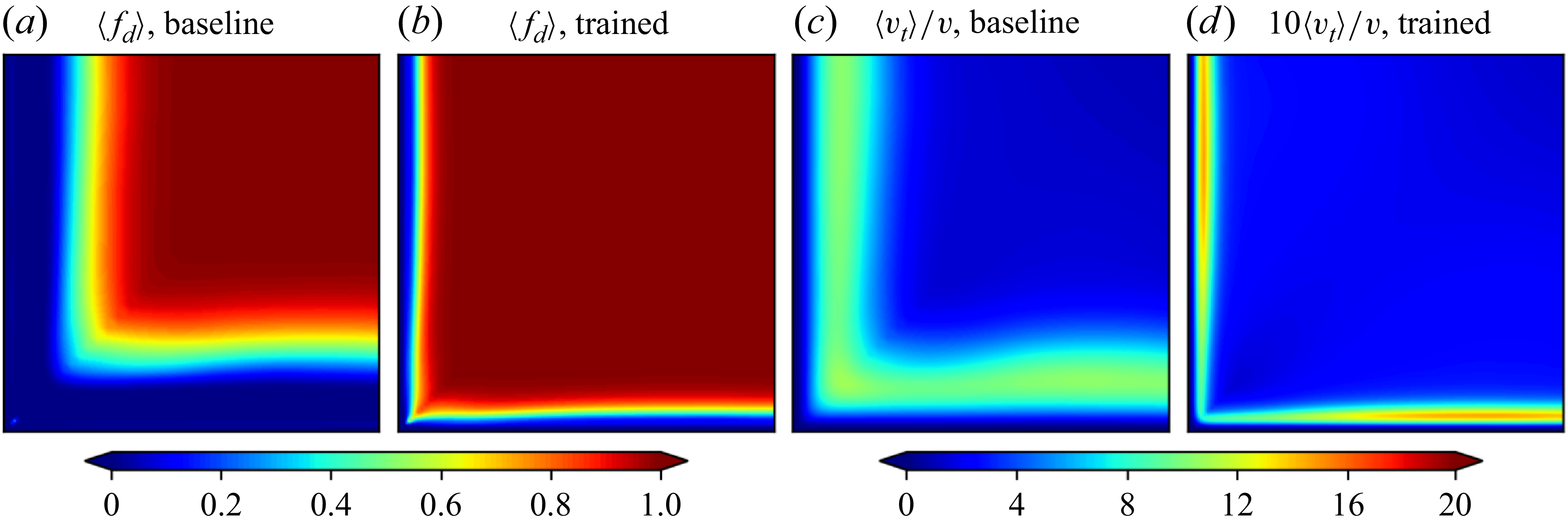
Figure 5 compares the switching behaviours between the RANS and LES branches for the baseline and the trained models. Specifically, the mean shielding function $\langle f_d \rangle$ is shown in figure 5(a,b), and the mean eddy viscosity ratio $\langle \nu _t \rangle / \nu$ is shown in figure 5(c,d). Strictly speaking, the shielding function $\langle f_d \rangle$ in DDES ensures a shielded near-wall RANS region to prevent the GIS issue. Outside the shielded region, the RANS and LES length scales ( $\ell _{\textit{RANS}}$ and $\ell _{\textit{LES}}$ ) are compared locally to determine the RANS/LES mode, as described in § 2.2. Usually, $f_d = 1$ alone does not sufficiently indicate a LES region. However, in the present square duct flow simulations, the mesh is sufficiently fine outside the shielded region ( $\Delta x^+ \approx 30$ and $\Delta y^+_{max } = \Delta z^+_{max } \approx 15$ ), ensuring $\ell _{\textit{LES}} \lt \ell _{\textit{RANS}}$ in these regions. Therefore, $f_d$ is sufficient to indicate the switching behaviour in this case.

Figure 5.

Comparisons of the shielding function $f_d$ and the turbulent viscosity ratio $\nu _t/\nu$ between the baseline EAS-DDES model and the trained DD-EAS-DDES model.

It can be seen that the trained model performs a much larger region of the LES branch as indicated with $\langle f_d \rangle = 1$ . The near-wall RANS region is much thinner than that of the baseline model. This leads to a relatively small eddy viscosity ratio for the trained model, compared with the baseline. Note that $\langle \nu _t \rangle / \nu$ for the trained model in figure 5(d) is scaled by a factor of 10 for clarity. These facts indicate that the trained model enhances performance by enlarging the LES region to resolve more turbulent structures.

To explore the underlying reasons for the trained model’s behaviour, the model coefficients $C_1$ , $C_2$ and $C_{\textit{DES}}$ , and the calculated $C_\mu ^*$ are examined. The relative variations of these model coefficients compared with the baseline values are presented in figure 6. As shown in figure 6(d), $C_\mu ^*$ in the near-wall region is lower than the baseline value, which is determined by the variation of $C_1$ and $C_2$ from the baseline value. This coefficient directly controls $f_d$ as (2.7). That is, a smaller $C_\mu ^*$ leads to a larger value of $f_d$ , consequently, a thinner shielded RANS region. Additionally, $C_\mu ^*$ and $C_{\textit{DES}}$ jointly control the production term of the $k$ transport equation as (2.1). The simultaneous decrease of $C_\mu ^*$ and $C_{\textit{DES}}$ reduces the modelled kinetic energy, which further increases $f_d$ . Therefore, both the variations of $C_{\textit{DES}}$ and $C_\mu ^*$ result in enlarging the LES region and resolving more turbulent structures.

Figure 6.

Mean values of the model coefficients $\langle C_1 \rangle$ , $\langle C_2 \rangle$ , $\langle C_{\textit{DES}} \rangle$ and $\langle C_\mu ^* \rangle$ of the trained DD-EAS-DDES model in the third quadrant ( $y\lt 0$ , $z\lt 0$ ) of the square duct. The coefficients are normalized by the baseline values.

To investigate the effects of the trained model coefficients, we present the resolved and modelled parts of the turbulent stress as shown in figure 7. From figure 7(a,b,e, f), the increasing trend of resolved TKE portions for the trained model can be seen. For the baseline model, the modelled TKE is primarily distributed in the near-wall region, and the resolved part is distributed away from the wall, with both exhibiting a similar maximum magnitude. While for the trained model, TKE is almost fully resolved, with the modelled part being small.

Figure 7.

Comparisons of the mean resolved and modelled parts of TKE and secondary shear stress between the baseline EAS-DDES model and the trained DD-EAS-DDES model in the third quadrant ( $y\lt 0$ , $z\lt 0$ ) of the square duct.

As discussed above, the secondary flow is mainly driven by the turbulent normal stress anisotropy $(\hat {\tau }_{yy} - \hat {\tau }_{zz})$ and the secondary turbulent shear stress $\hat {\tau }_{yz}$ . Specifically, the predictions of the baseline and the trained model have major differences in $\hat {\tau }_{yz}$ (see figure 4d,h,l). Figure 7(c,d,g,h) illustrate the resolved and modelled parts of $\hat {\tau }_{yz}$ for the baseline and trained models. For the baseline model, the modelled part accounts for a large proportion of $\hat {\tau }_{yz}$ , while the resolved part is relatively small. The spatial distribution of $\tau _{yz}$ is very similar to the total one $\hat {\tau }_{yz}$ (figure 4h), and the deviation from the DNS result mainly comes from the modelling error. In contrast, the major contribution of $\hat {\tau }_{yz}$ is from the resolved part for the trained model, which is similar to the distribution of the DNS result (figure 4d). This further confirms that the better performance of the trained model is mainly attributed to the increase in the resolved turbulence.

The variations of the coefficients $C_1$ and $C_2$ have two main effects on the model prediction. The first is to alter the switching location between the RANS and LES regions by modifying $C_\mu ^*$ . The second one is to alter the nonlinear extra anisotropy $\boldsymbol{a^*}$ by modifying the expressions of the tensor basis coefficients $\beta _i$ as listed in the Appendix A. To assess the contribution of the second effect, a new simulation is conducted by using the baseline $C_1$ , $C_2$ values, and the trained $C_{\textit{DES}}$ function. This can lead to a similar $f_d$ distribution as the fully trained model, while the functions of $\beta _i$ with respect to the scalar invariants $\theta _{\!j}$ are unchanged because of using the baseline $C_1$ and $C_2$ values. The results of the mean secondary velocity $\langle \bar {u}_y \rangle$ are shown in figure 8. Overall, the predictions from the partially trained case are similar to the fully trained case. A difference can be observed in the positive $\langle \bar {u}_y \rangle$ region near the central line ( $z=0$ ), as pointed by the black arrows, where the fully trained model has slightly better performance than the partially trained one. Hence, the modifications of $\beta _i$ functions with the trained $C_1$ and $C_2$ have positive effects on the model performance, although the impact is weaker than the modification of LES/RANS switching location via the trained $C_{\textit{DES}}$ .

Figure 8.

Comparison of the mean secondary velocity $\langle \bar {u}_y \rangle$ between the DNS, the fully trained DD-EAS-DDES model and the DD-EAS-DDES model with trained $C_{\textit{DES}}$ in the third quadrant ( $y\lt 0$ , $z\lt 0$ ) of the square duct.

4.4. Generalization in Reynolds number

The generalizability of the trained model is further assessed in two square duct flows of $\textit{Re}_b = 7000$ and 40 000. The mesh is the same as the trained case, which means the grid resolution relative to turbulence scales varies due to the variation of the Reynolds number, with a larger proportion of turbulent scales being modelled at a higher Reynolds number. As such, the model’s generalizability can also be assessed in the grid resolution with respect to the turbulence scales. The secondary flow predictions of the baseline and the trained models are compared with the DNS result in figure 9. A significant improvement in the accuracy of the trained model is observed for both cases, which is similar to the case of $\textit{Re}_b = 17\,800$ as shown in figure 2(f–h). The predicted locations of the positive and negative peaks of $\langle \bar {u}_y \rangle$ (as marked by the yellow symbols) are closer to the duct corner with the increase of Reynolds number, and the positive $\langle \bar {u}_y \rangle$ near the central line ( $z = 0$ ) is better predicted than the baseline model. Compared with the baseline model, the trained model’s absolute errors are remarkably reduced for both cases in the whole domain. Conclusively, the trained model can be well generalized to flows with this different Reynolds number.

Figure 9.

(a–c, f–h) The mean secondary velocity $\langle \bar {u}_y \rangle$ of the DNS result, the predictions by the baseline and trained EAS-DDES models and (d,e,i, j) the absolute errors for the baseline and trained models in the third quadrant ( $y\lt 0$ , $z\lt 0$ ) of the square duct flow with (a–e) $\textit{Re}_b = 7000$ and (f–j) $\textit{Re}_b = 40\,000$ . The model is trained in the square duct flow with $Re = 17\,800$ .

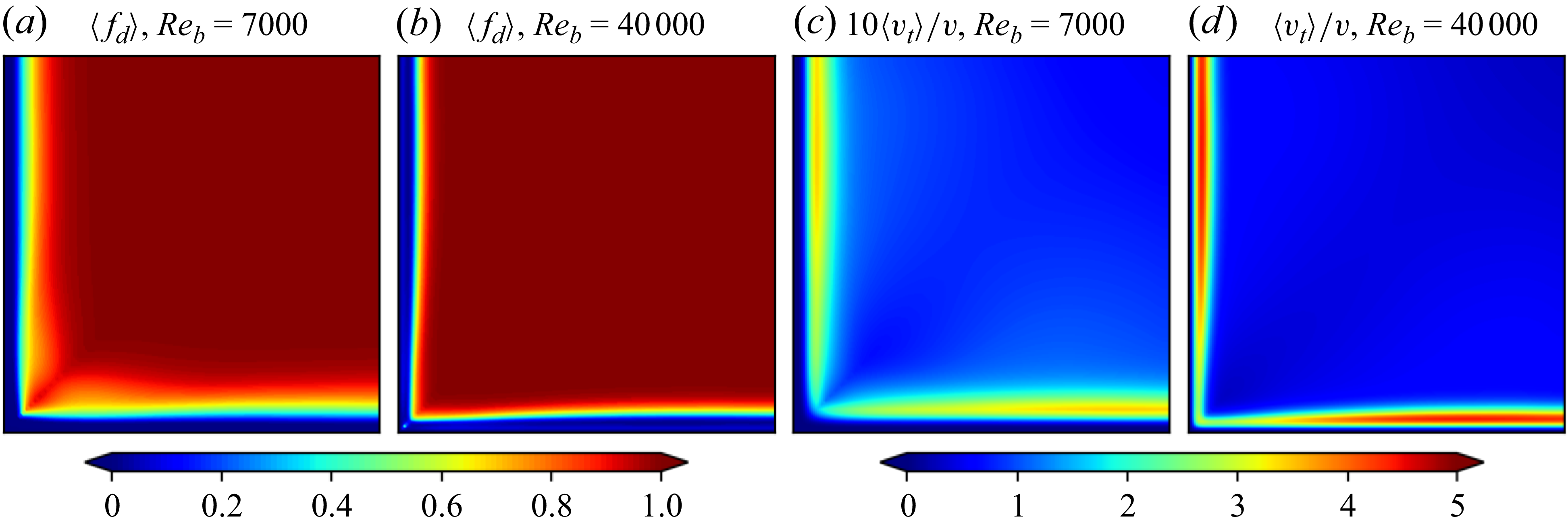
The switching behaviours of the trained model can be well generalized to the cases with different Reynolds numbers. It is supported in figure 10, which compares the switching behaviours of the $\textit{Re}_b = 7000$ and $\textit{Re}_b = 40\,000$ cases. Both cases are simulated based on the DD-EAS-DDES model trained by the $\textit{Re}_b = 17\,800$ case. The distribution of $f_d$ is almost unchanged for the two different Reynolds numbers, while the eddy viscosity ratio $\langle \nu _t \rangle /\nu$ in the near-wall RANS region becomes significantly larger for higher Reynolds numbers. For clarity, $\langle \nu _t \rangle /\nu$ is scaled by a factor of 10 for the $\textit{Re}_b = 7000$ case in figure 10(c). This indicates a larger proportion of modelled stress at higher Reynolds numbers.

Figure 10.

Comparisons of the time-averaged DDES shielding function $f_d$ and the turbulent viscosity ratio $\nu _t/\nu$ between the $\textit{Re}_b = 7000$ and the $\textit{Re}_b = 40\,000$ cases simulated by the trained DD-EAS-DDES model. The model is trained in the square duct flow with $Re = 17\,800$ .

5.1. Case set-up and numerical methods

The flow over the bump with $h = 38$ mm is chosen to train the DES model. The computational domain and mesh on the $xy$ plane are shown in figure 11. The length of the bump is $C = 305$ mm, which consists of a circular arc with a chord length of $(5/6)C$ and convex fillets with a radius of $0.323C$ added before and after the arc. The Reynolds number of the bump case is $\textit{Re}_c = 2 \times 10^5$ based on the free stream velocity and the bump length. Before the bump, the inlet section consists of two parts. The inlet section I with a length of $(2/3)C$ is added to ensure adequate development of synthetic turbulence introduced at the inlet. The inlet section II has a length of $C/3$ , which is consistent with the LES configuration. The outlet section length after the bump is $(2/3)C$ . The height of the domain is $C/2$ , and the width is $0.22C$ . The computational domain is the same as the LES case (Matai & Durbin Reference Matai and Durbin2019b) except for the inclusion of the inlet section I.

Figure 11.

The computation domain and mesh on the $x$ – $y$ plane for the separated flow over a bump.

The structural mesh consists of $0.42 \times 10^6$ cells, with 175, 60 and 40 cells in the streamwise, wall-normal and spanwise directions, respectively. In the streamwise direction, the grid is uniformly distributed for inlet section I and the bump region, with the cell size $\Delta x/C = 0.013$ and $\Delta x^+ \approx 100$ . For the inlet section II and the outlet section, the grid size is stretched in the streamwise direction by a factor of two towards the inlet and the outlet, respectively. In the wall-normal direction, the grid spacing is progressively refined towards the bottom wall, with the cell size of the near-wall first layer satisfying $\Delta y^+_1 \lt 1$ . The grid is uniformly distributed in the spanwise direction, with the normalized size $\Delta z/C = 0.0055$ and $\Delta z^+ \approx 40$ .

The periodic boundaries are set for the spanwise direction. The slip and no-slip boundaries are set for the top and bottom walls, respectively. The outlet is imposed with fixed pressure, zero velocity gradient and non-reverse flow. At the inlet, the velocity follows LES practice by adding synthetic turbulence to the mean velocity profile to obtain the instantaneous velocity. The synthetic turbulence is constructed by the synthetic digital filter method (Klein, Sadiki & Janicka Reference Klein, Sadiki and Janicka2003). It employs the digital filtering of random data to reproduce specified second-order (single-point) statistics and the autocorrelation functions of the velocity. The synthetic digital filter method has been widely used in generating desired inflow turbulence in eddy-resolving simulations (Wu Reference Wu2017). The required mean velocity, Reynolds stress and integral length profiles are provided by a precursor RANS simulation of a zero-pressure-gradient flat plate. The streamwise location $x_0$ with the same boundary layer thickness as the LES inlet is prescribed, and the profiles at $x = x_0 - (2/3)C$ are extracted for generating the inlet instantaneous velocity. For the turbulence properties, the $\omega$ profile is also extracted from the precursor RANS simulation of the flat plate. In the DES, $k$ represents the modelled part of TKE, which is set to zero at the inlet, and synthetic turbulence is introduced to represent the resolved TKE. The subgrid TKE is underestimated near the inlet, while it can be developed to a physical value after the inlet section I.

The numerical schemes are the same as the square duct flow case described in § 4.1. The time step size is fixed at a value with a maximum Courant–Friedrichs–Lewy number of approximately 0.5. The flow statistics are obtained by averaging over time and spanwise direction, with the averaging time interval $\Delta t_{\textit{av}} \approx 8 C/u_b$ .

In this case, the flow separation and reattachment are of primary interest. Given this, the training data are selected between the beginning of the bump ( $x/C = 0$ ) and the reattachment point ( $x/C = 1.1$ ) based on the LES in the $x$ direction. The range in the $y$ direction is $y \lt 0.2C$ . The observation region is shown as the blue dashed lines in figure 11. In this region, flow data are extracted along 23 parallel vertical lines with an interval of $0.05C$ in the $x$ direction. For all cells along these lines, the mean streamwise velocity divided by the local wall distance, $\langle \bar {u}_x \rangle / d_w$ , is used as the training data. Here, $d_w$ is introduced to compensate for the small velocity values near the wall, as suggested by Matai & Durbin (Reference Matai and Durbin2019b). The training data is also weighted by the local cell volume. As for the ensemble Kalman method, 16 samples are drawn in this case, which is the same as the square duct case. The convergence is achieved in approximately 20 iterative steps. In each training step, the computational cost for each sample is approximately 50 hr of CPU time (equivalent to the computational cost of the baseline or trained DD-EAS-DDES models in this case), resulting in a total training cost of 16 000 CPU hr.

5.2. Predictions of velocity and skin friction coefficient

Figure 12(a–c) shows the normalized mean streamwise velocity contours. Both the baseline and trained models are in good agreement with the LES data upstream of the bump crest, where the flow experiences a weak APG to FPG. However, in the region of strong APG after the bump crest, a substantial difference is observed in the predictions by both models. Compared with the LES result, the baseline EAS-DDES model predicts the separation point too early, leading to a significantly large recirculation zone. In contrast, the prediction of the trained model is in excellent agreement with the LES result. Both the separation and reattachment locations are accurately predicted.

Figure 12.

Comparisons of the normalized instantaneous and mean streamwise velocity contours and the Q-criteria contours at $Q = 2\times 10^5 \,\rm s^{-2}$ , between the (a,d) LES, (b,e) baseline EAS-DDES model and (c, f) trained DD-EAS-DDES model for flows over the bump.

Regarding the instantaneous streamwise velocity, as shown in figure 12(d–f), both the baseline and the trained models resolve the turbulent motions well before the bump crest. The main difference in the instantaneous velocity fields between the two models is located in the separated shear layer after the bump crest. The prediction of the baseline model exhibits a strong delay of transition from modelled to resolved turbulence in the separated shear layer, known as the ‘grey area’ issue in hybrid RANS-LES approaches (Probst et al. Reference Probst, Schwamborn, Garbaruk, Guseva, Shur, Strelets and Travin2017; Pont-Vílchez et al. Reference Pont-Vílchez, Duben, Gorobets, Revell, Oliva and Trias2021; Wang, Tang & Liu Reference Wang, Tang and Liu2025). In contrast, the trained model exhibits a reasonable development of the resolved turbulent motions in the shear layer. The resolved turbulent motions occur much earlier than the baseline model and are consistent with the LES results.

The comparison is also made in the instantaneous contour lines of Q-criterion, as depicted in figure 12(g–i). The blue lines denote $Q = 2\times 10^5 \,\rm s^{-2}$ , and the red lines mark $\langle \bar {u}_x \rangle /u_0 = 0.2, 0.8$ after the bump crest to indicate the separated shear layer. Both models predict larger turbulent structures than the LES due to the coarser mesh. With the trained model, the predicted turbulent motions occur immediately upon shear layer separation, which agrees with the LES result. In contrast, the baseline model suffers from the ‘grey area’ issue, predicting a strong delay in the occurrence of turbulent motions in the separated shear layer.

Figure 13(a,b) shows the mean velocity profiles in the streamwise and wall-normal directions. Before the bump crest, both models can predict the velocity profiles well. However, the baseline model exhibits large discrepancies from the LES after the bump crest due to the incorrect predictions of the separation and reattachment points. In contrast, the predictions of the trained model agree well with the LES results. Although only the streamwise mean velocity is used in the loss function during the training process, the wall-normal velocity is also accurately predicted by the trained model. This can be explained by the divergence-free constraint of the mean flow. That is, the accurate prediction of $\langle \bar {u}_x \rangle$ inherently improves the prediction of $\langle \bar {u}_y \rangle$ in this spanwise-homogeneous case with $\bar {u}_z=0$ .

Figure 13.

Comparisons of the mean and r.m.s. velocity profiles of the bump case between the LES, the baseline EAS-DDES model and the trained DD-EAS-DDES model at different streamwise locations with an interval of $0.2C$ .

The r.m.s. velocity profiles are also significantly better predicted with the trained model than the baseline model, as shown in figure 13(c,d). At $x/C = 0.8$ , the baseline model under-predicts the velocity fluctuations due to the delayed unsteadiness in the separated shear layer, as illustrated and explained in figure 12. Farther downstream, the velocity fluctuations are over-predicted due to the delayed reattachment of the separated shear layer. The trained model substantially mitigates these issues. This significant improvement is achieved without including r.m.s. velocities in the training loss, which further demonstrates the effectiveness of the present data-driven DES model.

Figure 14 illustrates the mean skin friction coefficient $C_{\!f}$ for flows over the bump. In the region of FPG ( $0 \lt x/C \lt 0.5$ ), the trained model accurately predicts $C_{\!f}$ in comparison with the LES result, while the baseline model over-predicts $C_{\!f}$ in the region of ( $0.2 \lt x/C \lt 0.5$ ), and the peak location of $C_{\!f}$ is delayed in the prediction of the baseline model. In the APG region before the flow separation ( $0.5 \lt x/C \lt 0.8$ ), there exists a local maximum of $C_{\!f}$ for the LES results, which is also observed in previous DNS of a Gaussian bump (Balin & Jansen Reference Balin and Jansen2021). The existence of a local maximum is also captured by the trained model, although the magnitude is lower than the LES result. In contrast, this local maximum is not observed in the prediction of the baseline model. After the flow separation ( $x/C \gt 0.8$ ), the predicted $C_{\!f}$ by the trained model agrees well with the LES results, indicating the accurate predictions of the flow separation, reattachment of the separated shear layer and the recovery of the reattached turbulent boundary layer farther downstream. In contrast, the friction coefficient $C_{\!f}$ predicted by the baseline model severely deviates from the LES results due to the significantly over-predicted area of the separation region, as shown in figure 12(d–f).

Figure 14.

Comparisons of the skin friction coefficient between the LES, the baseline EAS-DDES model and the trained DD-EAS-DDES model for flows over the bump.

The improvement of the predicted mean $C_{\!f}$ can be explained by the prediction of the turbulent stress. Based on mean friction drag decomposition in the turbulent boundary layer (Renard & Deck Reference Renard and Deck2016; Fan et al. Reference Fan, Li, Atzori, Pozuelo, Schlatter and Vinuesa2020; Elnahhas & Johnson Reference Elnahhas and Johnson2022), the contributions of the mean $C_{\!f}$ consist of a laminar part, turbulent momentum flux, streamwise growth of the boundary layer, mean wall-normal flux and the free stream pressure gradient. In consideration of the pressure gradient contribution, the free stream FPG and APG increase and decrease the mean $C_{\!f}$ by increasing and decreasing the free stream velocity, respectively, relative to the local boundary layer. This determines the variation of mean $C_{\!f}$ over the bump as shown in figure 14. The turbulent momentum flux contribution is determined by the turbulent shear stress in the wall frame $\hat {\tau }_\textit{tn} \equiv \langle u^{\prime}_t u^{\prime}_n \rangle$ , where the subscripts ‘ $t$ ’ and ‘ $n$ ’ denote the wall-tangential and wall-normal directions, respectively. In general, the increase of $\hat {\tau }_\textit{tn}$ leads to the increase of the mean $C_{\!f}$ .

Figure 15 depicts the distribution of $\hat {\tau }_\textit{tn}$ under the local wall frame in the near-wall region. In the range of $0 \lt x/C \lt 0.2$ , both models predict a slightly higher value of $\hat {\tau }_\textit{tn}$ compared with the LES results. In $0.2 \lt x/C \lt 0.6$ , the trained model predicts a low magnitude of $\hat {\tau }_\textit{tn}$ near the wall due to the presence of the FPG, which is close to the LES result. However, the baseline model predicts a much higher $-\hat {\tau }_\textit{tn}$ in this region (marked by the black arrow), resulting in an overestimated mean $C_{\!f}$ in this region. Farther downstream, the prediction of the trained model is similar to the LES results. A high turbulent shear stress region appears in the range of $0.6 \lt x/C \lt 0.9$ due to the strong APG effect, as marked by the blue arrows. This leads to the abrupt increase of mean $C_{\!f}$ and the occurrence of a local maximum, as shown in figure 14. The occurrence of this high $-\hat {\tau }_\textit{tn}$ region is slightly delayed for the trained model compared with the LES result, leading to the slightly delayed increase of the mean $C_{\!f}$ . The high $-\hat {\tau }_\textit{tn}$ region enables the near-wall flows to resist the strong APG and keep attached until $x/C \approx 0.8$ . As for the baseline model, the magnitude of $\hat {\tau }_\textit{tn}$ in the range $0.6 \lt x/C \lt 0.8$ is significantly under-predicted, leading to premature flow separation. Overall, the baseline model fails to accurately reflect the effect of the pressure gradient on Reynolds shear stress, resulting in inaccurate predictions of the separation point and the mean $C_{\!f}$ . In contrast, the trained model significantly improves the prediction of Reynolds shear stress, resulting in enhanced prediction performance.

Figure 15.

Comparisons of the Reynolds shear stress in the wall-frame between the LES, the baseline EAS-DDES model and the trained DD-EAS-DDES model for flows over the bump.

5.3. Switching behaviours and model coefficients

Figure 16(a,b) compares the mean shielding function $\langle f_d \rangle$ of the baseline and the trained models. Similar to the square duct case, the trained model reduces the near-wall shielded RANS layer in the region over the bump ( $x/C\lt 1$ ). As explained in § 4.3, $f_d=1$ does not necessarily mean the model is switched to LES, and this is true for the present case due to a moderate mesh resolution ( $\Delta x^+ \approx 100$ and $\Delta z^+ \approx 40$ ). Given this, we define the LES mode indicator $\phi$ as

(5.1) \begin{equation} \phi = \frac {\ell _{\textit{DDES}} - \ell _{\textit{RANS}}}{\ell _{\textit{LES}} - \ell _{\textit{RANS}}}, \end{equation}

to further demonstrate the switching behaviour. This indicator $\phi$ varies from 0 to 1, with $\phi = 0$ and $1$ corresponding to the use of RANS or LES length scale for $\ell _{\textit{DDES}}$ , respectively.

Figure 16.

Comparisons of the (a,b) mean DES shielding function $\langle f_d \rangle$ , (c,d) the LES mode indicator $\langle \phi \rangle$ and (e, f) the turbulent viscosity ratio $\langle \nu _t \rangle /\nu$ between the baseline EAS-DDES model and the trained DD-EAS-DDES model for flows over the bump.

The mean value of $\phi$ is shown in figure 16(c,d). In the region before the flow separation ( $x/C \lt 0.7$ ), the trained model has a higher value of $\langle \phi \rangle$ than the baseline model. This means that the trained model tends to resolve a larger proportion of turbulence scales to better predict the local turbulent state, yielding a significant improvement in the skin friction on the hump, as previously shown in figure 14. More importantly, the convection of resolved turbulent structures into the near-wall boundary layer enhances its resistance against strong APG, resulting in delayed flow separation and a more accurate separation point prediction. In figure 16(f), a clear, near-wall RANS layer is established after $x/C=1.0$ , which results in a good skin friction prediction after reattachment, as shown in figure 14.

Further, the resolved and modelled parts of the Reynolds shear stress are illustrated in figure 17. The solid line roughly indicates the RANS/LES switching location. For the baseline model, the near-wall RANS region is relatively thick. Moreover, the Reynolds shear stress in $0.2 \lt x/C \lt 0.6$ is over-predicted (pointed by the blue arrow in figure 17c), which can be attributed to the modelling error of the RANS branch in capturing the effects of the pressure gradient on the Reynolds stress. For the trained model, the near-wall flow in $0.2 \lt x/C \lt 0.6$ is largely resolved, and the effects of the pressure gradient can be effectively captured. Farther downstream, the strong APG significantly enhances the turbulent intensity, leading to an abrupt thickening of the near-wall RANS region. Before the separation ( $0.6 \lt x/C \lt 0.8$ ), the proportion of the modelled stress played a crucial role in the total stress, as pointed by the red arrow in figure 17(f). This indicates that the near-wall RANS model has non-negligible contributions to the improved prediction of the flow separation point in this case.

Figure 17.

Comparisons of the resolved and modelled Reynolds shear stress ( $\langle \bar {u}_t' \bar {u}^{\prime}_n \rangle / u_0^2 \times 10^3$ and $\langle \tau _\textit{tn} \rangle / u_0^2 \times 10^3$ ) in the wall-frame and the proportion of the modelled part $|\langle \tau _\textit{tn} \rangle | /(|\langle \bar {u}^{\prime}_t \bar {u}^{\prime}_n \rangle | + |\langle \tau _\textit{tn} \rangle |)$ between the LES, the baseline EAS-DDES model and the trained DD-EAS-DDES model. The solid line is the contour line of $\langle f_d \rangle = 0.5$ .

The trained model coefficients $C_1$ , $C_2$ and $C_{\textit{DES}}$ , and the calculated $C_\mu ^*$ are examined for this case to explain the model behaviour. The relative variations of the trained coefficients compared with the baseline values are shown in figure 18. The value of $\langle C_{\textit{DES}} \rangle$ is lower than the baseline value in the near-wall region before the separation ( $x/C \lt 0.7$ ). A smaller $\langle C_{\textit{DES}} \rangle$ predicted by the trained model leads to decreased subgrid viscosity (plotted in figure 16), and thus reduces the production of $k$ near the edge of the RANS region. The variation of $k$ can affect the RANS region thickness due to the dependency of $f_d$ on $k$ as in (2.7). This is the main reason for the reduction of the near-wall shielded RANS region. Additionally, the mean $C_\mu ^*$ is larger than the baseline value in the whole domain through the variations in $C_1$ and $C_2$ from their baseline values. This modification to the near-wall RANS model can play an important role in the strong APG region, due to the abrupt thickening of the near-wall RANS region and the increase in the modelled stress contribution, as demonstrated in figure 17. The relatively large $C_\mu ^*$ increases the near-wall shear stress in this region, enabling the flow to resist the APG and keep attached until the correct separation point. To summarize, the combined modifications of $C_{\textit{DES}}$ and $C_\mu ^*$ (modified through $C_1$ and $C_2$ ) lead to the effective response of the near-wall shear stress to the pressure gradient by enlarging the LES region in the FPG region and modifying the RANS model in the APG region, which improves the model prediction of the flow separation point and the skin friction.

Figure 18.

Mean values of the model coefficients $\langle C_1 \rangle$ , $\langle C_2 \rangle$ , $\langle C_{\textit{DES}} \rangle$ and $\langle C_\mu ^* \rangle$ of the trained DD-EAS-DDES model.

5.4. Generalization in similar geometries and different grid resolutions

The generalizability of the trained model is further examined by simulating flows over the bumps with different heights. Two different bump heights, i.e. $h = 26$ and 42 mm, are chosen, denoted by the h26 and h42 cases, respectively. The h26 case is marked as the ‘flow on verge of separation’ in the LES of Matai & Durbin (Reference Matai and Durbin2019b). The flows over the two bumps are simulated using the baseline and trained models, respectively, compared with the LES results. The employed trained model is trained from the h38 case with the bump height $h=38$ mm. The mesh quality is kept the same as the training case.

Figure 19 illustrates the normalized mean streamwise velocity $\langle \bar {u}_x \rangle / u_{0}$ . It can be observed that the baseline model predicts a premature separation and a delayed flow reattachment for both cases, which is similar to the observed features in the h38 case. The trained model predicts very similar flow patterns as the LES results for both cases. The separation and reattachment points of the h42 case are correctly predicted. The flow features on the verge of separation for the h26 case are also accurately captured with the trained model.

Figure 19.

Comparisons of the normalized mean streamwise velocity $\langle \bar {u}_x \rangle / u_{0}$ contours of the flow over the bump between (a,b) the LES, (c,d) the baseline EAS-DDES model and (e, f) the trained DD-EAS-DDES model for the h26 and the h42 bumps. The DD-EAS-DDES model is trained in the h38 bump case.

Figure 20 presents the predicted mean shielding function $\langle f_d \rangle$ and LES mode indicator $\langle \phi \rangle$ contours for the h26 and h42 bumps. These results closely match the performance observed in the training case (the h38 bump, shown in figure 16b,d). Therefore, the switching behaviour of the trained DD-EAS-DDES model can be generalized to geometrically similar configurations.

Figure 20.

The mean shielding function $\langle f_d \rangle$ and LES mode indicator $\langle \phi \rangle$ contours simulated by the trained DD-EAS-DDES model for the h26 and the h42 bumps. The DD-EAS-DDES model is trained in the h38 bump case.

In addition, the trained model’s generalizability has been assessed on a finer mesh, with the cell sizes halved in both the streamwise and spanwise directions, corresponding to $\Delta x^+ \approx 50$ and $\Delta z^+ \approx 20$ in the bump region. The cell size in the wall-normal direction is maintained. The DES is performed with the baseline and the trained models, where the latter is trained on the base mesh. The mean velocity profiles are depicted in figure 21. Similar to the base-mesh results, the trained model performs significantly better compared with the baseline model on the fine mesh, indicating the robustness of the trained DD-EAS-DDES approach under different mesh resolutions. It is also worth noting that for the trained model, the fine-mesh results are relatively less accurate than those on the base mesh, as shown in figure 13(a,b). This could be further improved by training the model with different mesh resolutions.

Figure 21.

Comparisons of the mean velocity profiles of the bump case between the LES, the baseline EAS-DDES model and the trained DD-EAS-DDES model at different streamwise locations with an interval of $0.2C$ . The DES cases are under the fine mesh, while the trained model is trained with the base mesh.

The switching behaviours of the trained model under different mesh resolutions are demonstrated in figure 22. The mesh resolution has negligible influence on the DDES shielding function $f_d$ . It is reasonable because the shielded RANS region is already very thin, especially on the bump surface. Since switching too close to the wall would cause premature separation, the trained model seems to sustain a robust shielding for the RANS region. In contrast to $f_d$ , the LES mode indicator $\langle \phi \rangle$ reflects the local proportion of the resolved turbulent scales. With finer meshes, the LES mode is more prone to be activated outside the near-wall shielded region due to the decrease of $\ell _{\textit{LES}}$ . This trend is well demonstrated by the plot of $\langle \phi \rangle$ in figure 22(c,d). Therefore, the trained model has a physically justified switching behaviour in the DDES framework.

Figure 22.

The mean shielding function $\langle f_d \rangle$ and LES mode indicator $\langle \phi \rangle$ contours simulated by the trained DD-EAS-DDES model for different mesh resolutions. The DD-EAS-DDES model is trained with the base mesh.