

1 Introduction
The valuation of liabilities of pension funds is in a state of flux. Traditional actuarial rules prescribe discounting of the expected cash flows at a fixed interest rate (typically 4%), although it is not always clear whether this should be applied to the nominal or indexed pension claims. Recently, due to changes in the supervisory and accounting rules, pension funds are required to value their liabilities at market prices. Typically, this is done by discounting the liabilities with a market interest rate for loans with the same maturity and risk characteristics. In practice, this approach poses some challenges, as pension fund liabilities are typically not marketed assets. The long maturity of the claims and, perhaps most importantly, the indexation to price or wage growth make it impossible to find a portfolio of perfectly matching market instruments. Therefore, finding the right discount rate is problematic.
In the literature on financial asset pricing (see e.g. Duffie, Reference Duffie1996), the situation where a payoff cannot be replicated perfectly using market instruments is referred to as a situation of an incomplete market. In such a setting, part of the payoff risk on the derivative is uncorrelated to the price changes in the replicating assets. Reasons why replication may be imperfect are the lack of traded instruments, infrequent (non-continuous) trading, and transaction costs. For the case of pension liabilities, the major source of market incompleteness is the absence of financial market instruments that exactly replicate the price or wage index to which the pensions are linked. Although there may be products that correlate strongly with the price level, such as index-linked bonds, this is definitely not the case for wage-linked payoffs. Hence, for the valuation of wage-linked pension liabilities, one cannot use a replicating argument directly.
The academic literature offers a few methods for the pricing of assets in incomplete markets. A first approach is to find a super-replicating portfolio, see e.g. Cvitanic, Pham, and Touzi (Reference Cvitanic, Pham and Touzi1998, Reference Cvitanic, Pham and Touzi1999). This is a portfolio whose payoffs are always (in any state of the world) at least as big as the payoff of the derivative. The value of the derivative is then bounded by the value of the super-replicating portfolio. Although for some products, such as options, this may be a useful approach; for pension fund liabilities, this approach is not very helpful as the unhedgeable wage growth is in principle unbounded and no super-replicating portfolio can be found.
A second approach, developed by Cochrane and Saá-Requejo (Reference Cochrane and Saá-Requejo2000), weakens the no-arbitrage argument and finds arbitrage strategies that have bounded Sharpe ratios. Cochrane and Saá-Requejo claim that even in incomplete markets, this argument may lead to very tight bounds on option values.
The third approach that we consider is a utility-based valuation. The investor in the pension liability assumes unhedgeable risk, which will affect the probability distribution of his consumption and final wealth level, and hence his utility. The certainty equivalent wealth of the expected utility then is the value an investor is prepared to pay for the claim. Conversely, we may ask how much wealth the pension fund should invest in the market to give their members the same utility as a fully guaranteed wage-indexed pension. This wealth then is the ‘shadow’ market value of the (partially) unhedgeable claim. This approach is an application of the utility undifference pricing methodology, introduced in dynamic asset allocation problems by Hodges and Neuberger (Reference Hodges and Neuberger1989) and surveyed by Henderson and Hobson (Reference Henderson, Hobson and Carmond2004).
The final approach we consider is suggested by He and Pearson (Reference He and Pearson1991) and Sangvinatsos and Wachter (Reference Sangvinatsos and Wachter2005). They propose to find a market price of risk that makes the (aggregate) demand for a newly introduced asset that completes the market equal to zero.
In this paper, we discuss these approaches to pricing in incomplete markets in more detail. We also and apply these methods to the specific case of pension liabilities, which have unhedgeable wage-indexation risk. We demonstrate that finding a value for the pension liability amounts to finding a value for the price of the residual wage risk. We show that this valuation method can be implemented in a simple way by adjusting the discount rate for pension claims. The methods suggested in this paper can also be used to price other financial instruments whose payoffs are linked to an index. Examples are TIPS, GDP bonds, and longevity bonds.
The organization of this paper is as follows. Section 2 provides a detailed introduction to the various valuation principles for incomplete markets. Section 3 applies these methods to the case of wage-linked assets and pension claims. Section 4 calibrates the valuation model to data from the Netherlands and the US. Finally, Section 5 draws some conclusions.
2 Valuation principles
The workhorse of asset pricing theory is the pricing kernel or stochastic discount factor.Footnote 1 This is a random variable that can be used to price any asset in the economy. The price of a contingent claim is given asFootnote 2
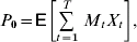
where X t are the (random) cash flows generated by the claim at time t and M t is the pricing kernel. It can be demonstrated that such a pricing kernel exists in any economy where the law of one price holds. If we also assume absence of arbitrage, the pricing kernel is always positive, i.e. a positive payoff will always have a positive price. The pricing kernel is not necessarily unique; there may be many Ms that give the correct prices. Only in the case where markets are complete the pricing kernel is unique.
An important example of a complete markets setting is the Black and Scholes (Reference Black and Scholes1973) asset-pricing model. In this model, the price of the basic asset (a stock) follows a geometric Brownian motion with expected return μ and volatility σ

In addition to this stock, there exists a risk-free asset with constant return r. Cochrane (Reference Cochrane2001) shows that the pricing kernel in this model is

where Zt is the Brownian motion driving the stock price, and λ is the Sharpe ratio of the stock

The interpretation for this pricing kernel is simple. The first part is the risk-free discount factor, and the second part is the random variable, which puts a high weight on payoffs that occur at low values of the stock (i.e. low values of Z t). The pricing kernel depends on the risk-free interest rate, which captures the time value of money, and the Sharpe ratio of the stock, which captures the risk–return tradeoff for stock market exposure. This property holds more generally: with multiple sources of risk in the economy, the stochastic discount factor can typically be written as a function of the risk-free rate, the Sharpe ratios of marketed assets and the shocks to the asset prices, and λ and dZ t are vectors of Sharpe ratios and stochastic shocks, respectively. The dynamics of the SDF are given by

With this pricing kernel, any contingent claim with payoff X t=f(S t) can be priced by calculating the expectation

In the Black–Scholes example, there is only one source of uncertainty, the stock price, and the market is (dynamically) complete, since the payoff of any stock price derivative can be attained by a trading strategy in the stock and the risk-free asset. This is of course a very stylized setting and, in practice, the payoff of claims such as pension liabilities depend on a multiple of risk factors. Moreover, some of these risk factors cannot be replicated by trading in financial market instruments. How to deal with pricing and valuation in such a situation?
2.1 Good deal bounds
One guideline for the valuation of claims in an incomplete market is given by Cochrane and Saá-Requejo (Reference Cochrane and Saá-Requejo2000) (CS from now on).Footnote 3 Suppose the uncertainty in the payoffs is generated by the stock price from equation (2) and an additional state variable V, whose dynamics can be described by

where Z tw is a Brownian motion that is independent of Z t. The coefficients σV and σVw denote the exposure of the state variable V to the stock price shocks and the independent Brownian motion.
CS show that the pricing kernel in this economy has dynamics

where, as before, λ is the Sharpe ratio of the stock and λw is an unknown coefficient. In an incomplete market (where there are no traded assets that correlate with Z w) the no-arbitrage framework does not pin down the value of λw, so that we are left with an infinity of possible SDFs and, by implication, infinitely many possible values for contingent claims that depend on the value of the state variable V. The insight of CS is that λw can be interpreted as the Sharpe ratio of a (hypothetical) asset that has a non-zero exposure to dZ tw and no exposure to dZ t. Now CS suggest to put a bound on the absolute value of this Sharpe ratio, such that too ‘good deals’, i.e. assets or positions with too high (absolute) Sharpe ratios, are ruled out. The bounds on the Sharpe ratio then imply an upper and lower bound for the value of any contingent claim. Of course, the magnitude of the bound on the Sharpe ratio is arbitrary, but CS show that even fairly generous values for the bound may lead to very tight ranges for the implied prices of derivatives such as options. In Section 3.1 we analyze this method for the case of wage-indexed pension claims.
2.2 Utility-based pricing
An alternative approach to pricing in incomplete markets is based on the utility a representative agent can derive from investing in the untraded claim. This approach has been used extensively in the literature, for example by Svensson and Werner (Reference Svensson and Werner1993), Henderson (Reference Henderson2002, Reference Henderson2005), and Chen, Pelsser, and Vellekoop (Reference Chen, Pelsser and Vellekoop2007). These papers study a situation where a new derivative is added to the existing portfolio of an investment bank or a new product is added to the portfolio of an insurer, and part of the risk on the new derivative or product cannot be hedged using market instruments. Our analysis builds on these papers and is also closely related to work on asset allocation in incomplete markets, see for example the work by Brennan and Xia (Reference Brennan and Xia2002), Munk and Sørensen (Reference Munk and Sørensen2007), and De Jong, Driessen, and Van Hemert (Reference De Jong, Driessen and Van Hemert2007). We now first discuss the general setup of the utility maximization problem and outline how it can be used to find the value for a non-traded claim. In Section 3 we present a detailed model that is explicitly targeted at valuing long-dated pension claims.
The setting we study is a stylized representation of an individual saving for retirement. The main simplification is that we consider a terminal wealth problem and ignore intermediate consumption and labour income. Thus, the economic agent maximizes expected utility of terminal wealth over all the possible investment strategies. First consider the complete markets problem, where any value of terminal wealth can be attained by an investment strategy in financial market instruments. In that case, the agent solves the problem

where U(W) is the utility function, W 0 the initial wealth, M 1T is the pricing kernel for the marketed risks, and the latter condition is the budget constraint. From the mathematical finance literature (see e.g. Cox and Huang, 1989, and Pliska, Reference Pliska1997) it is well known that the optimal investment strategy is given by

where ℓ1 is the Lagrange multiplier of the budget constraint.
For the incomplete markets setting, in general, finding the optimal investment policy is a hard problem and an optimal wealth strategy cannot be derived using the Cox–Huang method. However, we assume a particular structure on the utility function and the risk, such that the problem can be simplified enough to apply these methods. First, assume that terminal wealth can be decomposed as the product of a perfectly hedgeable wealth component W 1T and an independent component W 2T. The additional term W 2T can be interpreted as exogenous background risk; here it is assumed that the stochastic processes W 1 and W 2 are independent. The agent then solves the problem over all feasible values for W T, subject to a budget constraint

The optimal wealth strategy can be derived from the first-order condition

so that

We now have all the ingredients to find the equivalent utility price of the unhedgeable risk. Define the expected utility of complete markets problem as

With background risk, the expected utility is

Hence, to obtain the same expected utility as in complete markets case, an additional fraction of initial wealth π has to be invested, with

We work out the value for π for the case of wage-indexed pensions in Section 3.2.
2.3 Equilibrium pricing kernel
An alternative way to find the value of a claim in incomplete markets follows an argument by He and Pearson (Reference He and Pearson1991) and Sangvinatsos and Wachter (Reference Sangvinatsos and Wachter2005). They suggest completing the market with a new instrument to hedge the previously unhedged risk and augmenting the pricing kernel with the new risk factor; then choosing the additional parameter of the pricing kernel such that the demand for the new instrument equals exactly zero. This pricing kernel parameter will determine the equilibrium market price of risk of the additional risk factor and thus the market price of the new instrument. This approach will be applied to wage-indexed pension claims and wage linked bonds in Section 3.3.
3 Wage risk
In this section, we apply the equivalent utility pricing principle to the case of unhedgeable real wage risk. We first present a specific model for a long-horizon investor who faces wage growth risk. The objective of the consumer is to maximize the utility of wage-deflated terminal wealth.Footnote 4 This is different from the Brennan and Xia (Reference Brennan and Xia2002) model, where the agent maximizes the utility of price-deflated wealth. This is our way of introducing wage risk into the model. The optimization problem is

subject to a budget constraint, where W T denotes undeflated wealth and Y T denotes the wage level.
The stochastic model for financial market prices and wages is similar to the model of Svensson and Werner (Reference Svensson and Werner1993). The model has a stock return and wage growth equation. We allow for time-varying interest rates. This is important, as pension claims are long-dated and pension funds therefore face large interest rate risks. The equations driving these variables are



where the vector Z=(Z S, Z r) and the covariance matrix of dZ is ρ. In the last equation, Y is the wage-index level and g denotes the expected wage growth. The term θ′dZ denotes the exposure of wage growth to the shocks in stock returns and interest rates. The final term θwdZ w denotes the idiosyncratic wage risk, which is by assumption uncorrelated with the other risk factors. We assume that in the economy there are stocks and a full menu of bonds, so that interest rate risk can be hedged perfectly, but there are no traded wage linked assets. Asset values are determined from the pricing kernel

where φ=−ρ−1λ and λ=(λS, λr)′ is the vector of market prices of risk or Sharpe ratios. Brennan and Xia (Reference Brennan and Xia2002) show that the price dynamics of a T period zero-coupon bond are

with B(T) a function of the time to maturity T of the bond, that follows from the Vasicek (Reference Vasicek1977) model
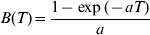
To simplify the analytical results, we assume that all volatilities, market prices of risks and correlations are time invariant. Hence, interest rates are normal, and stock and bond returns, as well as wages, are log-normal. We furthermore assume that the expected wage growth is constant over time. The model can easily be extended to serially correlate expected wage growth, at the expense of more heavy notation.
3.1 Good deal bounds
The good deal bounds of Cochrane and Saá-Requejo (Reference Cochrane and Saá-Requejo2000) can be easily applied to the wage risk setting, but as the wage growth indexation applies to the full value of the liabilities, the implied bounds can actually be pretty wide. To give an example, suppose that wages are not correlated with stock prices and interest rates (θ=0) and the Sharpe ratio of wage-linked assets is bounded by |λw|<A. Then the discount rate to be applied to the payoff of a wage-linked bond is bounded between (r−g−Aθw, r−g+Aθw), where θw is the idiosyncratic volatility of wage growth. Estimates in Section 4 show that the interest rate minus the wage growth (r−g) is around 1.5%, and the annualized variance of the idiosyncratic wage growth is 4.5%. We choose A=0.2, which corresponds roughly to the equity market Sharpe ratio.Footnote 5 With these numbers, the discount rate is in the range (0.6%, 2.4%). Assuming a liability of 100 million euro with a duration of 20 years, this implies a range of present values between 62.23 and 88.72 million, roughly a 50% difference. This is a fairly wide range and may be too wide to get good judgements of the solvency of the fund.
3.2 Utility-based valuation of wage risk
For the utility-based valuation, we return to the utility maximization problem in equation (17). The optimization problem with explicit budget constraint is

where M 1T is the pricing kernel for tradeable wealth, denoted by W T. The wage level is decomposed as Y t=Y 1tY 2t, where Y 1 denotes the part of wage growth that can be spanned by traded assets, and Y 2 the orthogonal part.Footnote 6 The dynamics of the wage components therefore are


According to Brennan and Xia (Reference Brennan and Xia2002), the optimal wealth strategy W T* is independent of Y 2T because this is just independent background risk that cannot be hedged and therefore does not affect the optimal wealth strategy.Footnote 7 Solving for the optimal wealth process gives

where ℓ is solved from the budget constraint. The indirect utility function therefore can be written as

Using that  , we find

with
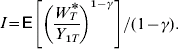
Notice that I is the indirect utility of the complete markets (θw=0) problem, which is independent of the parameters for Y 2T. The certainty equivalent wealth of the optimal portfolio strategy is

Hence, to achieve the same certainty equivalent wealth in the incomplete markets case, we need to invest a fraction  more than in the complete markets case. Notice that π>1 if γ>2, so it is only for moderately risk-averse investors that the elimination of idiosyncratic wage risk is welfare improving.Footnote 8
This result can be used to price wage-linked bonds. According to the previous argument, such a bond is valued by an agent who wants to hedge wage risk. This agent requires a per-period risk premium  for the idiosyncratic wage risk; notice that this additional risk premium is negative for γ>2, so that relatively risk-averse investors are willing to give up expected return to get exposure to the wage risk. The return on a fully indexed pension (or wage-linked bond), paying off Y(T) at time T, then must be

with
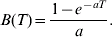
The first part of the expected return, r−B(T)σrλr, is the yield on a T period non-indexed zero-coupon bond. The term θ′λ reflects the risk premium earned on the ‘best’ (but imperfect) hedging portfolio of stocks and bonds for the wage-linked bond.Footnote 9 The remaining term,  , is the risk premium for idiosyncratic wage risk.
The expected real return on a wage-linked bond is the appropriate discount rate for fully indexed pension claims. From the bond return equation (29), the expected real return can be easily derived as

with  the vector of risk premiums corrected for correlation with wage growth. The expected real return is lower than the expected (nominal) return on an equivalent non-indexed bond by the expected wage growth g; this is similar to the classic Gordon stock valuation model, where the discount rate equals the cost of capital minus the expected dividend growth. The expected real return is also different because of the correlations between wage growth and the other risk factors,
 , which depends on the risk premium on the other risk factors. Finally, the expected real return has an extra term for the market incompleteness. This term is always negative.
The model of Bodie, Merton, and Samuelson (Reference Bodie, Merton and Samuelson1992) is a special case of this model, where there is no idiosyncratic wage risk, i.e. θw=0. Svensson and Werner (Reference Svensson and Werner1993) show, in a CARA-normal framework, that the discount rate for wage-linked claims is

where Γ is the coefficient of absolute risk aversion. The additional discount for wage risk is positive, because in their model utility is not scaled by the wage level but by the price index. Hence, a position in a wage-linked asset adds to uncertainty instead of providing a hedge against fluctuations in deflated wealth.
3.3 Equilibrium pricing kernel for wage risk
Sangvinatsos and Wachter (Reference Sangvinatsos and Wachter2005) suggest to find the equilibrium price of wage risk by completing the market with a new instrument to hedge the previously unhedged wage risk, and to choose the additional parameters of the pricing kernel such that the aggregate demand for new instruments equals exactly zero. In this section, we work out this approach. The advantage over the utility-based approach is that we can easily derive the equilibrium price in an economy that consists of agents with different preferences or different amounts of human capital.
Introduce an asset that spans the previously unhedged real wage risk. When such an asset exists, the pricing kernel can be extended to

Adapting the results of Brennan and Xia (Reference Brennan and Xia2002) and De Jong (Reference De Jong2008), the optimal portfolio weights are given as

where σ is the matrix of exposure coefficients of the assets included in the portfolio problem, and  is the correlation matrix of (dZ, dZ w)′. The first component of expression for the optimal portfolio weight is the usual mean–variance optimal speculative portfolio. The second component contains the hedges against wage risk and interest rate risk.
To simplify the algebra, consider a hypothetical asset that has a positive exposure to the idiosyncratic real wage risk and no exposure to the other sources of risk. The return on this asset is given by

with λw=−φw. With this wage-linked asset as the last asset in the vector x, the weight on the wage-linked instrument in equation (34) simplifies to

The principle of Sangvinatsos and Wachter (Reference Sangvinatsos and Wachter2005) is to find a value φw such that the demand for wage-linked bonds is zero, hence x w*=0. The solution to this equality is

For γ>1, the pricing kernel parameter will be positive, and hence the implied risk premium on the new asset, λw=(1−γ)θw, will be negative.
In this complete market, the price of a long maturity wage-linked bond (WLB) with maturity T obeys

The expected real return of the wage-linked bond therefore follows as

There is a small difference with the result based on the equivalent utility argument, equation (31): the additional discount for idiosyncratic risk is γθw2 and not  . This difference is explained by the fact that under the Sangvinatsos–Wachter argument, the investor optimally chooses a position in WLBs, whereas in the equivalent utility argument, the original position in assets is augmented with WLBs such as to compensate for the utility cost of the unhedged risk.
The argument so far considered a single investor who invests all his wealth in financial assets. In reality, even investors have a fraction of their wealth locked up in human capital. The Appendix shows that the demand for the wage-linked asset for an investor with human capital to total wealth ratio h satisfies

In an economy with many agents, setting the aggregate demand for the wage-linked asset equal to zero and solving for the pricing kernel parameter gives

where 1/γ* is the wealth-weighted average risk tolerance in the economy and h* the aggregate human capital to total wealth ratio. The intuition for this result is quite simple. The hedge demand for wage-linked assets is positive for every agent. In equilibrium with a zero net supply of wage-linked assets, this hedge demand has to be compensated with a negative speculative demand, and therefore φw+θw is positive in equilibrium. With this equilibrium risk premium, investors with high risk aversion or low human capital (typically these are the older investors) will have a positive net demand for the wage-linked asset, whereas investors with low risk aversion or high human capital will short the wage-linked asset. The equilibrium discount rate for wage-linked bonds then follows as

4 Calibration
In this section, we calibrate the model with real-wage growth to data from the Netherlands and the US.
4.1 Netherlands
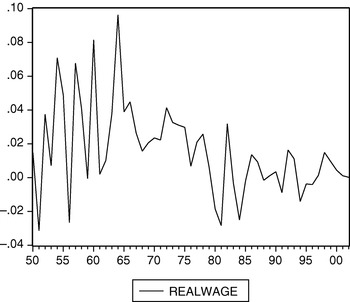
For the Netherlands, the sample period is 1950–2002 (annual data), obtained from Statistics Netherlands. Real wage growth is constructed as nominal wage growth minus realized inflation, and is graphed in Figure 1. The wage growth fluctuates quite a bit and also exhibits some persistence, i.e. years with high wage growth are more likely to be followed by another year of high wage growth. The mean and standard deviation of annual wage growth are 1.5% and 2.65%, respectively. The sum of the coefficients in an AR(3) model (selected by the Akaike information criterion) is 0.55, indicating some persistence in the wage growth process. As this persistence is not explicitly taken into account in the model of this paper, we correct the standard deviation of wage growth to correspond to the annualized standard deviation of the 30-year wage growth. For this, we use the formulas of the variance ratio in Campbell, Lo, and MacKinlay (Reference Campbell, Lo and Craig MacKinlay1997: 49). Corrected for serial correlation, the annualized standard deviation of wage growth is 4.5%.
Real-wage growth in the Netherlands
This figure shows annual real wage growth rates in the Netherlands, 1950–2002.

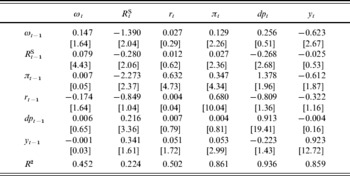
The exposure coefficients θS and θr are estimated using the residual covariance matrix of a VAR(1) model for excess stock returns, the expost real interest rate (constructed as the difference between the nominal short rate and inflation) and the real-wage growth. The estimates are reported in Table 1. These estimates imply a positive but small exposure of wage growth to stock returns and interest rates. Using an equity Sharpe ratio of 0.2, the stock market exposure translates into a risk premium of θSλS=0.0030∗0.20=0.0006, or only 6 basis points, which is almost negligible.Footnote 10 The real interest rate exposure is also small and leads to a negligible addition to the risk premium.
Selected parameter estimates
This table shows selected estimates of the parameters in the model, obtained from annual data for the Netherlands, 1950–2002. The subindex S refers to the excess stock return, r to the expost real interest rate (nominal short-rate minus inflation) and w to real wage growth.

To give a numerical example, assume a risk aversion γ=5 and an idiosyncratic wage risk θw=4.5%, based on the estimate of real-wage volatility corrected for serial correlation. We assume a real interest rate of 3% and an expected real-wage growth of 1.5%. The discount rate for wage-indexed pensions then is
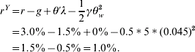
The additional term caused by the market incompleteness is −0.5%, which seems small, but with such low interest rates it has a significant impact on the valuation. The shadow market value of the 100 million liability from the earlier example will be 81.95 million. Ignoring the extra term of the market incompleteness (i.e. assuming a discount rate of 1.5%), the value is 74.25, which makes about a 10% difference.
4.2 US
Next, we calibrate the model to US data. As wages in the US exhibit more nominal rigidity than in Europe, the model is estimated including inflation and nominal t-bill rate as additional determinants. Moreover, we include the dividend–price ratio, whcih is a well-known predictor of stock returns. Finally, we include the logarithm of the dividend to wage ratio; this follows follow Benzoni, Collin-Dufresne, and Goldstein (Reference Benzoni, Collin-Dufresne and Goldstein2007) who use this variable as a predictor for wage growth.
The wage data (Wage and Salary Disbursements) are from the National Income and Product Accounts (NIPA), collected by the Bureau of Economic Analysis of the Department of Commerce. Other data are stock returns (value weighted index including dividends), interest rates (annual returns on 90-day t-bills), CPI inflation and annual dividends (all these variables are obtained from CRSP). Following Heaton and Lucas (Reference Heaton and Lucas2000), we use postwar data, starting in 1946; our sample ends in 2006.
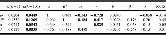
To estimate the long-run variances of these variables and their correlations with wage growth, we follow Campbell and Viceira (Reference Campbell and Viceira2005) and estimate a vector autoregression on stock returns, interest rates, inflation, and nominal wage growth. The VAR estimates are reported in Table 2, and Table 3 reports the implied long-run variances and covariances, calculated using the expressions in Hoevenaars et al. (Reference Hoevenaars, Molenaar, Schotman and Steenkamp2007). The estimates imply a long-run standard deviation of 4.5% for real wage growth, with positive exposures to stock market returns, a small exposure to inflation, and a negative exposure to interest rates. The magnitude of the exposures is most easily discussed using the beta's of the wage growth, which are obtained form a hypothetical multivariate regression of the long-run wage growth shocks on (long-run shocks to) stock returns, interest rates, and inflation. The stock return beta is 0.187. The inflation beta is close to zero and the (nominal) interest rate beta is −0.25. This may indicate that even in the long run there is some nominal rigidity in wages. The long-run annual standard deviation of the idiosyncratic wage growth is 2.4%.
VAR estimates for US data
This table shows estimates of a VAR on real-wage growth, ωt, stock returns, R S, interest rates, r, CPI ination, π, log dividend yield, dp t and the log wage–dividend ratio, y t, using annual data for the US over the period 1947–2006. T-statistics are given in brackets, σe is the standard error of the equation.

Long-run variances, correlations and risk premiums
This table shows the long-run standard deviation of the four variables, the exposure coefficients θ of the wage growth to the standardized innovations, the beta (βi=θi=σi). The Sharpe ratios λ are assumed values, except for λw, which is calculated as  for γ=5. The final column μ shows the contribution of each factor to the risk premium on a long maturity wage-linked bond (in excess of the risk premium on a long-maturity nominal bond), calculated as 100θλ (i.e. expressed as percent per annum).
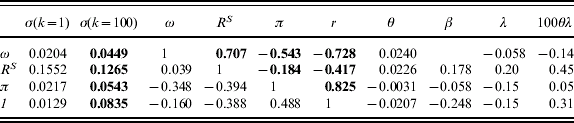
We calculate the risk premiums associated with the various sources of risk. For this exercise, we assume a market price of risk of 0.2 for stock returns, −0.15 for interest rate risk, and also −0.15 for inflation risk. The stock market risk contributes 45 basis points per annum to the risk premium of a bond linked to the nominal wage index. The inflation risk premium is negligible, but the interest rate risk premium is around 30 basis points. Finally, the premium for the idiosyncratic wage risk is small, around −15 basis points for an investor with risk aversion γ=5. All in all, the risk premium on a wage-linked bond is 60 basis points higher than the risk premium on a CPI indexed bond, mainly due to the positive stock market exposure of wages.
5 Conclusion and implications for pension funds
Pension funds with wage-indexed liabilities face two issues in valuating their liabilities. The first is that the expected wage growth has to be taken into account. This can be achieved fairly simply by correcting the discount rate for the expected wage growth rate. The second issue is more complex and arises because wage risk cannot be hedged perfectly. In other words, the pension fund cannot replicate a wage exactly with its asset mix. Although the asset mix may be chosen strategically to include assets that show correlation with wage growth, a non-hedgeable residual wage risk remains. Then, to offer the pension fund members the same expected utility as a perfect wage-indexed pension, the fund should invest initially more money (and hence pay out more on average) to compensate for this risk. In this paper, we show that this additional value can be calculated fairly easily by adjusting the discount rate of the future claims. We calibrate that the adjustment for the idiosyncratic wage risk is between −15 and −50 basis points. This effect is counterbalanced by the positive exposure of wage growth to the stock market, however, so the net adjustment to the discount rate will be higher and may even be positive.
Appendix: Portfolio demand with human capital
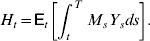
This appendix derives the optimal portfolio for an investor with human capital in a complete markets setting. Define human capital as the present value of the stream of future labor income
The wage process from equation (18c) is

with  and d
 =(dZ, dZ w)′. With the pricing kernel written as

where  , human capital equals

where r t(s) is the yield at time t on a bond with time to maturity s, and  are the market prices of risk. The dynamics of human capital are then

where B H is the interest rate duration of human capital, defined as

In a complete financial market, the optimal wealth strategy of the investor is determined from

The actual wealth dynamics for portfolio weights x are given by

with  is the fraction of human capital in total wealth. Equating these two expressions gives the optimal portfolio weights

with  . With the asset menu containing the hypothetical wage-linked asset with price dynamics (35), the corresponding element of equation (52) simplifies to

Now consider an economy with i=1, … , N individuals with risk aversion coefficient, γi total wealth W i, and human capital to wealth ratio h i. The aggregate demand for the wage-linked asset then is

Equilibrium with zero net supply of the wage-linked asset implies

or, equivalently

with