

1 Introduction
Phonology, and grammar in general, has been viewed in discrete computational terms since at least Pāṇini, whose grammar of Sanskrit is effectively a formal rewrite system (Ingerman Reference Ingerman1967). With the ease of modern programming environments and our fast personal computers, every theoretical phonologist can now implement and test their theories – as Karttunen (Reference Karttunen, Butt, Dalrymple and King2006) demonstrates, even quite simple theories may not actually do what their author intended. Such uses of computation raise no new problems for phonology or phonologists in the generative tradition; they merely let us do more of what we have done for two millennia, and faster.
During the twentieth century, increasing ease and power of computation also encouraged the use of simulation studies in phonology (and language more generally) such as the use of continuous parameters in vowel phonology, the use of probabilistic and stochastic models, models of phonological change based on agents and models of phonological learning in the individual. Such models may not have deterministic, repeatable results, and may not even have results easily amenable to statistical analysis; and the techniques required for analytical study may be quite mathematically sophisticated (such as the construction and numerical solution of sets of partial differential equations). When building simulations, there are many choices to be made about how much, and in which aspects, to abstract away from details of reality, and the effect of different abstractions and simplifications may not be clear. The consequence is that many simulation studies show at best that theory X is a possible account of phenomenon Y.
More ambitiously, if simulations are designed with careful analysis of the underlying theories, analyses of the sources of error, and the rest of the apparatus usual in physical and engineering science simulation studies, and then simulations are conducted over a wide range of possible configurations and parameter settings, one might establish with some confidence what is not possible, as well as what is possible; and one may even produce numerical results, testable for the degree of agreement with empirical data.
This article considers some case studies of the use of computational simulations and simulations of computational theories in phonology, critically examines what conclusions can be drawn from them and discusses new simulations inspired by this examination.
The title comes from a long folklore tradition of jokes about physicists and applied mathematicians: Q: How does a physicist milk a cow? A: Consider a spherical cow … .
2 Models and modelling
Science (and indeed pre-scientific explanations of the world) is fundamentally a process of constructing more or less abstracted models of reality, positing entities (atoms, quarks, thunder gods) whose existence explains something and (once thinking becomes scientific) making predictions from the model and validating them against reality.
There is a large literature on the notion of models and modelling in science – Frigg & Hartmann (Reference Frigg, Hartmann and Zalta2017) provide an overview, as well as pointers particularly into the philosophical literature. Space does not permit much discussion of this, but there are some (fuzzy) dichotomies of models that we will mention.
Marr (Reference Marr1977) proposes a dichotomy between ‘type I’ problems, where it is possible to construct a simplified or abstracted model and compute with it, such as the ideal model of gases or the phonemic theory of sound systems, and ‘type II’ problems, where there is no solution simpler than the problem itself. His example of the latter is protein folding, which was then and is still insoluble by any means other than a detailed simulation of atomic interactions. In the discrete computational world, the halting problem is a type II problem: the only general way to see if a program terminates is to run it until it does. It often appears that the agent-based models I discuss here are themselves type II problems, as they involve interactions of many processes; however, it is sometimes possible to abstract and approximate, as mentioned above.
Another distinction commonly made in the computer science modelling literature is that between discrete models and continuous or hybrid models. Any model involving real numbers cannot be stepwise simulated exactly, and issues of rounding and precision arise; on the other hand, techniques of mathematical analysis can make exact statements about entire regions of the model space in a way that is less common in discrete models. Most phonological simulation models are hybrid (discrete state plus continuous variables), and while there is a large literature on the analysis of such models, particularly in computer science, the techniques are non-trivial.
Finally, I should say that I will use the term abstraction in a narrow sense of intentionally removing detail, rather than in the broad sense of mathematising reality. (In the broad sense the Standard Model of particle physics, like every model, is thus an abstract model, but in the narrow sense it is not, as, despite its known incompleteness, the model does not intentionally omit any detail. On the other hand, a simple harmonic oscillator model of a pendulum does intentionally omit real details.)
3 The case of vowel systems
The first case study is the evolution of vowel systems, which provides examples of several dangers and difficulties that arise in the process of constructing models and drawing contentful conclusions from them.
3.1 Early models: dynamical systems
Modelling of vowel systems goes back to the early days of modern computing, when Liljencrants & Lindblom (Reference Liljencrants and Lindblom1972) placed points in a 3D formant-frequency space, imposed the constraint that points should try to ‘contrast’ (i.e. be as far apart as possible in perceptual space) and simulated the resulting dynamical system. The resulting arrangements of points achieved a reasonable level of match – judged impressionistically – with real vowel systems, although with a number of discrepancies: for example, predicting [ɨ] rather than the more frequent [ø] in seven- and eight-vowel systems. The conclusion was that ‘contrast’ is an important constraint determining the shape of human vowel systems.
This early model already demonstrates the importance of a key factor in all mathematical modelling of real-world systems: how abstract shall we be, and why are we making various abstractions, and does the resulting loss of fidelity in the modelling vitiate the conclusions? Is it safe to assume a spherical cow? Liljencrants & Lindblom make several abstractions that are repeated in the later work discussed below. I list some of them here, together with prima facie criticisms, which I examine more carefully in what follows.
(i) Vowels are represented by the first three formant frequencies. Despite debates on formant vs. whole-spectrum perception, the issues of speaker variation, etc. (see e.g. Johnson Reference Johnson, Pisoni and Remez2005), there is, and was, enough evidence for the key role of formants in vowel perception that this decision is likely to be accepted by most.
(ii) The boundaries of vowel space are defined by constructing a model of the vocal tract and basic articulators (Lindblom & Sundberg Reference Lindblom and Sundberg1969), to match ‘a typical male speaker’, and computing the possible formant frequencies emitted by this model. This is not justified over the alternative of using data from actual speakers; it was perhaps simply easier at that time to use their existing model to generate extremes than to use humans.
(iii) The acoustic vowel space is mapped to a perceptual space by converting Hertz to mels. The justification is that mels are by definition constructed to match the response of the human auditory system, and this should also apply to our perception of formants. However, over the range of frequencies that formants take, the non-linearity of the mel scale is not very marked, so it is not clear that this step had any significant effect on the results. (There was, indeed, existing work (Stevens Reference Stevens1952) suggesting that a linear scale might anyway have been better.)
(iv) The authors need a measure of how widely dispersed – how contrastive – a set of vowels is, in the perceptual space. They choose the measure in (1), where rij is the Euclidean distance between vowels i and j.
-
(1)

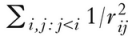
This is justified by analogy with physics, where many problems about bodies interacting via forces are solved by minimising the potential energy induced by the forces. In fact, their analogy fails, since the potential energy is the integral of the forces – contrary to their stated intention, they are using a 1/r3 force, penalising close-by vowels very strongly. It is not discussed whether the choice of a 1/r measure instead of a 1/r2 measure would have a significant effect.
(v) ‘To make computations somewhat easier’ (Liljencrants & Lindblom Reference Liljencrants and Lindblom1972: 841), the 3D space is projected down to a 2D space using F1 and a linear combination of F2 and F3 (still in mel space). On the face of it, this should make a dramatic change: confined to a 2D circle, the minimum energy configuration of four points is a square, whereas, confined to a 3D sphere, it is a tetrahedron, which might project to a quadrilateral, or to a triangle with an internal point, depending on the projection.
(vi) Finally, the results of letting this system evolve until it appears to have reached equilibrium are compared with the distribution of real-world vowel systems. However, these systems are of course generally reported only at the coarse level of one or maybe a half division on the standard IPA vowel chart. Matching of the ‘predicted’ system to real systems is impressionistic.
This short and incomplete list illustrates several of the reasons for making abstractions, and also several of the dangers. (i) is a simplification of complex reality, but with good evidence that the simplification should preserve behaviour. (ii) and (iii) are cases where a more detailed realisation is chosen for the sake of matching ‘reality’ better, but without an argument that the increased fidelity is needed. (iv) represents a poorly motivated choice for what may or may not be a critical function needed by the model. (v) shows a simplification purely to make the problem more tractable, with some justification from psychological reality, but one that may considerably change the behaviour of the system. (vi) demonstrates the difficulty of comparing even a very abstracted mathematical model with data obtained by others for their own, descriptive linguistic, purposes.
The model is conceptually simple, and aims simply to demonstrate that human vowel systems try to maximise contrast (learners of Danish may be forgiven scepticism). In fact, it is sufficiently conceptually simple that the entire numerical simulation set-up is unnecessary. One can reason analytically that, given a 1/r2 potential and the convex boundary shape, as the number of vowels increases, they will distribute around the boundary until the centre becomes nearer to an edge than the distance between vowels on the edge. Indeed this applies to a 1/r potential, or even any potential corresponding to a repulsive force, which shows that their accidental mismatch with physics was not important. At this point, centralised vowels appear, and typically there will be many minimal configurations – in a circular space, this happens when the sixth and seventh vowels are added. Which one Liljencrants & Lindblom's (deterministic) simulation arrived at will have depended on arbitrary factors of precision and rounding. With modern computing power, variation due to such factors is easy to explore; with the resources of 1970, it was not – their calculations, which would now take a fraction of a second, ran overnight.
It is, then, not clear that the entire paper says much more than ‘if vowels are subject to a pressure to contrast, they will be arranged to maximise contrast’, which is almost a truism. More importantly, the reverse implication, which is what the paper is aiming to establish, does not follow. To show what was claimed, the authors would need to have shown that if there is no pressure to contrast, then human vowel systems do not arise. It is trivial that without contrast or any other constraint, their model would allow random vowel systems; but it is not trivial to show that there is no other constraint than contrast which might lead to the human configurations.
I do not, of course, doubt that maximising contrast is a major factor in the shape of vowel systems, but Liljencrants & Lindblom (Reference Liljencrants and Lindblom1972) provided no substantive support for that belief, which rested quite adequately on informal considerations of communicative efficiency.
3.2 An agent model
As modern computing developed, it became possible to make effective use of models based on many interacting particles (e.g. nuclei) or elements (e.g. cells of atmosphere, or portions of an aircraft wing). The social sciences were quick to experiment with such models, with linguistic simulations appearing as early as Klein (Reference Klein1966). In such models, the term ‘agent’ refers to a process modelling some kind of human (or animal) actor, and which typically interacts with many other agents all running independently. In this subsection, I consider one of the best-known fairly recent phonological examples, again looking at vowel systems.
De Boer (2001) created a model, not of abstract synchronic vowel systems where one is looking for a defined ‘optimal’ system, but of speakers transmitting vowel systems through the generations. The basic framework is the ‘imitation game’ described by Steels (Reference Steels1997), which is an instantiation of a framework going back at least to early 20th-century work in population genetics. As applied by de Boer, the key points, and key abstractions are:
(i) A population consists of a number of agents.
(ii) Each agent possesses an inventory of ‘vowels’, identified as points in a 3D ‘articulatory’ space modelling height, backness and rounding.
(iii) Agents interact by events in which: (a) A chooses a vowel V from its inventory; (b) A ‘says V to B’: transforms V into a 3D ‘acoustic’ space (modelling the first three formants), and transmits it to B; (c) B transforms the acoustic signal to a 3D ‘perceptual’ space (essentially formants modified by mel and other psycho-acoustic results), and matches it against B’s own inventory (by ‘saying its vowels to itself’ and seeing which is the best match, according to the Euclidean distance in perceptual space), identifying a vowel V′; (d) B says V′ back to A; (e) A matches V′ against its own inventory, and signals ‘extralinguistically’ to B whether it heard V, the vowel it first sent; (f) if there was a match, B marks a successful communication against V′, and moves V′ somewhat in the direction of V (that is, reinforcement learning); if there was no match, B marks a failure against V′.
(iv) From time to time, agents spontaneously add a new randomly situated vowel to their inventory, remove repeatedly unsuccessful vowels, and merge vowels that are perceptually ‘too close’ together.
(v) Some random noise is added at all places where it can be: in the positions of the selected vowels, and at transformations between spaces.
Given this setting, a population of a dozen or two agents is allowed to interact for a few hundred or thousand transactions, and then the inventories of the agents are examined to see how well they match human systems – by impressionistic comparison of pictures. It is claimed that plausibly human-looking vowel systems emerge from this procedure.
Following the discussion in the previous subsection, it will be apparent that this work also contains some decisions that might be ‘bad abstractions’, or ‘bad non-abstractions’, as well as ‘good abstractions’ or ‘good non-abstractions’ (by non-abstraction, I mean a deliberate decision to retain some detail). De Boer does discuss some of these issues at some length, though without, in my view, complete success (see also Donegan's Reference Donegan2004 review for a critical view). One of de Boer's most interesting sections occurs only in his original thesis (Reference Boer1999: §3.1): he first tried to use a fairly concrete articulatory model, similar to that of Liljencrants & Lindblom, to generate not only the boundaries of the vowel space, but also the formant values. Moreover, he also tried to model consonants and distinctive feature phonology. This (hugely ambitious) project resulted in sound systems with ‘no relevance whatsoever to understanding human sound systems’ (1999: 27), and he scaled his ambitions back to the simpler model outlined above. Why did the first model fail? I am confident it was because of the uncontrollable interactions of bad abstractions and bad non-abstractions.
De Boer (2001) has been influential. It also sparked my own interest in simulations in phonology, and consequently I decided to examine it more closely, by re-implementing his framework and attempting to tease apart which abstractions and non-abstractions were good or bad. This I discuss in the following subsections.
3.3 Detail, parameters and abstraction in simulation
I re-implemented the framework of de Boer (Reference Boer2001) in Java. Thanks to de Boer's careful descriptions, this was for the most part straightforward.
One aspect of simulation models that I have not yet mentioned explicitly is the role of parameters. Almost every model will end up containing a number of numerical values or functions which encode choices not determined by the underlying theory. In the Liljencrants & Lindblom (Reference Liljencrants and Lindblom1972) model, examples include the strength of the contrast measure, the details of the projection from 3D to 2D, the precise details of the numerical hill-climbing algorithm, and so on. De Boer was unusually careful about mentioning these, but nonetheless missed one (at least; I added only those parameters essential for the model). There are a dozen parameters, and there is no really principled choice of value for most of them.
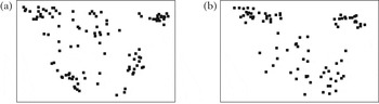
Figure 1 shows two example runs of my implementation of de Boer's (Reference Boer2001) original model, plotting the vowels of 20 agents, each starting with a single random vowel, after a few thousand interactions. In Fig. 1a, ‘standard’ parameter settings (copied from de Boer) have been used. The community has more or less converged on a five-vowel /i a ɨ ~ ə o u/ system. For the particular parameter settings used, four or five vowels are typical; by tweaking parameters, fewer or more vowels can be induced to emerge. However, in Fig. 1b, one parameter, artEpsilon, has been increased a little; this governs the amount by which successful listeners accommodate their vowel to what they heard. Here, /i u/ are reasonably clear, but there is no convergence in the lower half of the vowel space, and indeed more detailed inspection shows speakers with anywhere from four to ten vowels in their inventory.
Two runs of the de Boer (2001) algorithm, with different parameters.

This set-up, with its repeated, extensively randomised interactions, is not easily amenable to direct analysis in the way that Liljencrants & Lindblom's was. It is possible that hybrid system techniques or continuous approximation techniques could be applied, but this has not been done. The set-up has been treated as a type II model, whether or not it is one. Despite this, and although de Boer was explicit in avoiding the teleological ‘contrast-maximising’ inherent in Liljencrants & Lindblom (Reference Liljencrants and Lindblom1972), we might still ask whether anything can be learned from the simulation. The explicit biases in the model are to converge with one's peers, and to maintain the identity of phonemes until they become too close together. Implicitly, however, the convergence, together with deletion and merging, fairly directly have the effect of biasing toward contrast. As for the shape of the vowel systems, that these match (somewhat) with human vowel systems is a simple consequence of contrast being a function of distance in the vowel space, which makes vowels disperse just as much as Liljencrants & Lindblom's explicit potential function. In some ways, this model would be more interesting if it failed.
3.4 When are details necessary?
Having established the original model, we can ask which of its details are necessary to the results. In particular, the model has a fairly detailed model of transformations between (pseudo-) articulatory, acoustic and perceptual space. Is this detail of any importance? That is, when we've modelled a basically spherical cow, is there any point in modelling its several stomachs, rather than just having one tube? To investigate this, I produced a simplified version of the model. I threw away almost all the phonetic detail: vowels become simply points inside the unit height/backness/rounding cube, and are transmitted to the listener with no change other than the addition of noise. The only concession was to compress the perceptual front–back dimension of lower vowels, and reduce the size of the rounding dimension, to match the shape of the usual vowel chart, and so make merging more likely in low vowels.
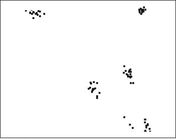
Figure 2 shows a run of the simplified system; parameter settings are mostly the same as in Fig. 1a, save that the perceptual parameter has been adjusted for the new space. One can see that this population has mostly settled on a five-vowel system, /i ε ɑ ɔ u/, which is both more tightly grouped and more human-looking than that in Fig. 1 (though there's a noticeable [a–ɑ] split in the /a/ vowel).
A run of the simplified model.

The sceptical reader will for some time have been asking a rarely addressed question: are these pictures cherry-picked? Let me be honest. Of course they are, as they almost certainly are in every simulation study ever published (apart from those who do carefully present composite data on many simulations). However, they are reasonably representative of typical runs, judged impressionistically. The sufficiently interested reader can run the programs to see – source code is available in online supplementary materials.Footnote 1
With more experimentation, it turns out that, at least to my eyes, the simplified model produces ‘more human’ vowel systems not just for five-vowel systems, but for higher numbers of vowels also. It is tempting to conclude, therefore, that de Boer's fairly detailed articulatory–acoustic–perceptual model was a ‘bad non-abstraction’ – retaining fidelity to reality gives less persuasive results. This is a somewhat disturbing conclusion, as indeed de Boer must have been disturbed when his first, ambitiously detailed, model, gave very poor results. We must hope that the cause lies in inaccuracy of the details, rather than in the decision to retain details.
However, an alternative to being disturbed is to ask whether we can learn something from the more abstract solution giving a better fit. This leads on to my second case study.
4 Inferring abstractions from simulation
4.1 Learning prototypes or features?
Boersma & Chládková (Reference Boersma and Chládková2010) were interested in whether people learn vowels as prototypes – that is, /e/ is a point in phonetic space which identifies the ‘best’ /e/ – or whether it can be argued that people learn to discriminate categorical features, so that /e/ is indeed a feature bundle.
Boersma has for some years been developing a sophisticated phonological grammar, one slogan of which is ‘bidirectionality’: the grammar is layered into modules, which feed up and down to each other. The grammar is constraint-based, in the style of Optimality Theory (Prince & Smolensky Reference Prince and Smolensky1993), though some of the constraints used are rather different from those of typical OT phonology: for example, so-called ‘cue constraints’ allow the specification of a vowel by weighting its formants against a large number of points on the frequency spectrum, and thereby allow vowels to be modelled as diffuse, distributional entities rather than points.
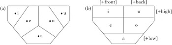
Boersma & Chládková (Reference Boersma and Chládková2010) set up a simulation framework in this grammar, with agents learning a five-vowel system, by re-weighting constraints on the basis of input. They report that when they simulate learners who are learning prototypes, the perceptual boundaries of the agents (as determined by testing them on an array of vowels) are drawn ‘diagonally’. On the other hand, if the learners are learning to associate vowels with [±high], [±back], etc., then the boundaries are horizontal and vertical. This is illustrated schematically in Fig. 3.
Vowel-perception boundaries in (a) prototype and (b) feature models, after Boersma & Chládková (2010).

Savela (Reference Savela2009) carried out extensive experiments testing the perceptual boundaries of vowels for speakers of many different languages, using artificial stimuli. The results appear to support horizontal/vertical divisions, rather than diagonal divisions. Thus, Boersma & Chládková say, their simulations support the claim that people learn features, not prototypes.
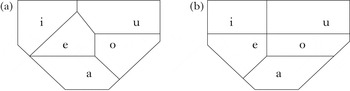
There is also a more specific claim about two languages. Spanish and Czech both have standard five-vowel systems. It is, however, claimed that Spanish phonology makes /a e/ [central], while in Czech /a/ is [back] and /e/ [front]. Running simulations learning these feature specifications predicts different perceptual boundaries, shown in Fig. 4. Boersma & Chládková conducted perception studies on Czech and Spanish speakers, and their results matched Fig. 4. (Clearly, they are assuming ternary height and backness features.)
Predicted boundaries in (a) Spanish and (b) Czech, after Boersma & Chládková (2010).

4.2 Analysis and response
We can make two criticisms of the argument, both of which echo criticisms made above of Liljencrants & Lindblom (Reference Liljencrants and Lindblom1972). The first is that the simulations add nothing to the argument. If agents model vowels as prototypical points, and incoming vowels are matched by Euclidean distance to the nearest such point, the boundaries in Fig. 3a are natural. Similarly, if they learn features that are defined to be horizontal and vertical divisions of vowel space, the boundaries in Fig. 3b are natural. The second is that, even granting the argument that the empirical results are consistent with feature learning, there might be other plausible explanations that would give similar results. In particular, could a different ‘prototype’ learning model account for the facts? I explored the latter by refining the simplified de Boer model introduced above. Recall that in this model, vowels were essentially points in abstract vowel space, with no subtleties of articulation or acoustics, and a minor adaptation for perception to compress low vowels. To explore the question, I made two changes to the model.
(i) Because we wish to study the evolution of the realisation of a stable vowel system, rather than the development of vowel systems, I split the population into adults (whose systems do not change) and children, who learn their vowels by interaction with adults according to the imitation game. As adults age and die, children replace them to maintain the population, and then become adults.
(ii) I enriched the notion of vowel, loosely inspired by exemplar theory (Pierrehumbert Reference Pierrehumbert, Gussenhoven and Warner2002). However, rather than exemplar clouds for words, or even phonemes, I proposed a simple model in which, for a vowel V, agents have an articulatory prototype for V, but also a convex polygonal region of space encompassing vowels they have heard and recognised as V by nearest matching. The prototype is nudged by the examples they hear; but the perceptual recognition region only expands.
(iii) I ignored the rounding dimension for this simulation.
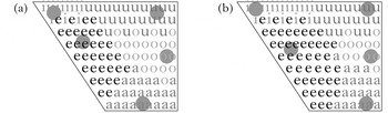
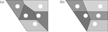
I also went back to the literature to investigate Spanish and Czech vowels (Harmegnes & Poch-Olivé Reference Harmegnes and Poch-Olivé1992, Ekštein Reference Ekštein2004, Volín & Studenovský Reference Volín and Studenovský2007, Chládková et al. Reference Chládková, Escudero and Boersma2011). I did not find strong support for the claim that Czech /a/ is [back]; indeed, some argue it is [central] (Aleš Bičan, personal communication). I did, however, find that a typical realisation of Czech /a/ is somewhat backer than Spanish /a/, that Spanish /e/ is typically higher than Czech /e/, and that the participants in Savela (Reference Savela2009) showed a similar slight difference in their judgement of the ‘best’ examples. Figure 5 shows schematically perceptual boundaries and best examples from Savela (Reference Savela2009), and Fig. 6 shows Fig. 4 adapted to the usual vowel quadrilateral.
Perception of (a) Spanish and (b) Czech vowels, adapted from Savela (2009). Synthesised vowels are plotted in acoustic F1, F2 space; the symbols indicate how humans classified vowels at each point. The grey circles mark the locations judged to be the ‘best’ representatives of the five vowels.

Results from Boersma & Chládková (2010), redrawn on the standard vowel quadrilateral: (a) prototype learning; (b) feature learning. The shaded areas indicate the perceptual regions after training. The white circles show the centres of the vowel distributions used in training.

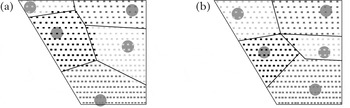
I converted average formant data from the sources to positions on the abstract vowel chart, and used these positions to seed the articulatory prototypes for ‘Czech’ and ‘Spanish’ populations. After running the simulation for a few generations, I measured the perceptual spaces of the agents. The results, together with the original prototypes, are shown in Fig. 7.
Agent simulation of vowel learning in the prototype and perceptual region model, with (a) Spanish and (b) Czech prototypes. The grey circles mark the locations of the prototypes in the initial populations. The shaded squares demarcated by black lines show the perceptual regions of an instance of a new adult after a few generations.

It is immediately noticeable that the rather small difference in the positions of the prototypes has a noticeable effect on the perceptual regions that agents acquire; that, in particular, the apparent slope of some region boundaries is changed from fairly diagonal to fairly horizontal; that, in general, the shape of these boundaries is not clearly identifiable as more similar to simple prototype-learning predictions than simple feature-learning predictions; and that the results match the empirical results of Savela (Reference Savela2009) rather well, particularly given the purely geometrical notion of vowel I use.
I have to admit that these results surprised me. The prototype-and-perceptual-region model is sufficiently complex that a simple qualitative analysis is not obvious, but my intuition was that the perceptual polygons would approximate circles, and the perceptual boundaries would end up in much the same place as before.
To summarise, I have here argued that two simulations with contrary intents give similar results, so that the original simulation does not itself argue strongly for feature-based perception. Of course, there are other ways to argue for it, and Chládková et al. (Reference Chládková, Boersma and Benders2015) have recently presented an elegant perception discrimination experiment which provides direct evidential support for the perception of features, so vindicating their original contention.
5 Discussion
In the foregoing, I looked at a sample of simulation work on a common theme, spanning forty years. I have suggested that in most of these, the simulations actually add little to the content of the work. Many other examples could have been adduced. Of course, I am not alone in this view; in discussions at conferences and elsewhere, many have agreed with my scepticism. But what can simulations do? When are they useful? Why does phonology (or linguistics) have a problem, when simulations are so widely used in the rest of science?
Firstly, what can simulations do? Most phonological simulations are designed to show that some theory or model could describe (or explain) some phenomenon. Simulations are very good at this: if you do a simulation of imitation-based learning, and end up with roughly human vowel systems, you can indeed conclude that imitation-based learning could be the reason for the shape of human vowel systems. So, however, could all the other uncountably many theories; and equally, countless variants of your pet system will not give the right results. It is rare to see a phonological simulation study that concludes that a particular range of models cannot account for a phenomenon, which would be a significant scientific contribution.
Part of the reason for this is obvious enough: the difference between the science underlying simulations in phonology and simulations in the physical sciences. In much of physical science, our model of reality is superbly accurate (quantum electrodynamics famously matches experiments to ten or twelve significant figures), and moreover our models appear to be ‘real’, in the sense that their structure corresponds exactly to the structure of reality – our fundamental models are both intensional and unabstracted, although we also know that they are wrong! In the physical sciences, simulations are used almost entirely to calculate things that simply cannot be calculated by analytic means. A typical example is weather, or even climate: though in principle we understand nature at the level of molecules and below, the complex and usually chaotic interactions of many entities make direct analysis utterly impossible. Simulations make very crude spherical cow-type abstractions – dividing the atmosphere into kilometre-sized blocks – but even so, the abstracted entities also have highly reliable models (ideal gas dynamics, with corrections), which in turn can be derived from and validated against the ‘real’ models. It is also the case that physical and biological scientists routinely use millions of times the computational resource available to linguists (e.g. millions of CPU hours to simulate one microsecond of the motion of one molecule).
In more human applications, such as modelling traffic flows to solve congestion problems, the model is much cruder, whether it is differential equations (crude because continuous) or interacting agents (much less complex than real drivers). Nonetheless, the model can be validated against large amounts of observational data; and need not be accurate. Many stochastic simulations have 20% errors compared to the real system; but that may be good enough for the purpose at hand (for example, city traffic models done in my department).
In phonology, however, we have no equivalent of the Standard Model, or even of ideal gases. We have many competing models, none of which is evaluable with precise numerical rigour against reality, and none of which addresses more than a small part of phonology and phonetics. Even in small areas, if we try to make detailed models, we often end up with Cthulhu cows, as de Boer did in his first attempts.
What can we get from simulations? Possibility demonstration is not useless: if the model is modestly complex, the fact that it can describe or account for some phenomenon may not be clear. An example of this is the demonstration in §4.2 that a non-feature learning system with a slightly richer vowel model can match data as well as a feature-learning system.
To make stronger statements, it is necessary to spend more time and effort on analysis of theories and methodologies. A recent example is Kirby (Reference Kirby2010), which studies the effect of phonetic cues on phonological (re-)categorisation, and is notable for using real acoustic data, as well as for a fairly sophisticated representation. Another is Sóskuthy (Reference Sóskuthy2013), which studies the notoriously difficult actuation problem, considering the interplay of phonetic biases with categorical effects, and contains an unusually detailed analysis both of the underlying theories and the expected accuracy of the simulations. Nonetheless, even these careful studies do not produce strongly constraining results.
To repeat my thesis from the introduction, if simulations are designed with careful analysis of the underlying theories, analyses of the sources of error, and the rest of the apparatus usual in physical and engineering science simulation studies, and then simulations are conducted over a wide range of possible configurations and parameter settings, one might establish with some confidence what is not possible, as well as what is possible; and one may even produce numerical results, testable for agreement with real empirical data.
Q: How does a phonologist hear a cow? A: Consider a binary feature vector … .