1 Introduction
The statics and dynamics of liquid droplets in wedge geometries constitute an active research topic across disciplines, including biological physics (Prakash, Quéré & Bush Reference Prakash, Quéré and Bush2008), granular media (Bocquet, Charlaix & Restagno Reference Bocquet, Charlaix and Restagno2002; Kohonen et al. Reference Kohonen, Geromichalos, Scheel, Schier and Herminghaus2004; Grof, Lawrence & Štěpánek Reference Grof, Lawrence and Štěpánek2008) and microfluidics (Renvoisé et al. Reference Renvoisé, Bush, Prakash and Quéré2009; Dangla, Kayi & Baroud Reference Dangla, Kayi and Baroud2013; Luo & Heng Reference Luo and Heng2014). More fundamentally, understanding the motion of droplets in wedges can shed light on complex phenomena, such as interfacial instabilities (Al-Housseiny, Tsai & Stone Reference Al-Housseiny, Tsai and Stone2012; Keiser et al. Reference Keiser, Herbaut, Bico and Reyssat2016) and the impact of surface roughness on contact-line dynamics (Moulinet, Guthmann & Rolley Reference Moulinet, Guthmann and Rolley2002).
When a liquid droplet is brought into contact with the inner walls of a wedge-shaped channel, the system will tend to minimise its total surface energy. In general, the transient dynamics and the final equilibrium state of the droplet can be characterised in terms of two main parameters, corresponding to the opening angle of the wedge,
 $\unicode[STIX]{x1D6FD}$
, which characterises the confinement geometry, and the equilibrium contact angle of the liquid with the solid,
 $\unicode[STIX]{x1D703}_{e}$
, which quantifies the wetting properties of the liquid.
Broadly speaking, one can identify four qualitatively different regimes for the behaviour of droplets in wedges, depending on the interplay between
 $\unicode[STIX]{x1D6FD}$
and
 $\unicode[STIX]{x1D703}_{e}$
, as summarised in figure 1. The first corresponds to a complete invasion regime, where
 $0^{\circ }\leqslant \unicode[STIX]{x1D703}_{e}\leqslant 90^{\circ }-\unicode[STIX]{x1D6FD}$
. In such a case the liquid–gas interface is concave and forms a transient capillary bridge when placed between the walls of a wedge. It was first noted by Hauksbee (Reference Hauksbee1710) that the free motion of such structures (i.e. in the absence of external forces, such as gravity) always results in their migration towards the apex of the wedge. Concus & Finn (Reference Concus and Finn1969) and Concus, Finn & McCuan (Reference Concus, Finn and McCuan2001) showed that a global equilibrium is not possible. Instead, the liquid prefers to spread along the apex of the wedge. Recently, Reyssat (Reference Reyssat2014) studied the motion of completely wetting capillary bridges (
 $\unicode[STIX]{x1D703}_{e}=0$
) within wedge-shaped channels and identified two regimes in the dynamics of the liquid. Close to the apex, the main source of energy dissipation is the viscous friction in the bulk of the liquid, which balances the rate of work done by capillary forces. As a result, the time evolution of the position of the capillary bridge is linear. This picture changes when the liquid is far from the apex of the wedge, where the main source of dissipation is the corner flow near the apparent contact lines. The result is a different equation of motion, which is given by a power-law dependence of the position of the liquid as a function of time with an exponent
 $4/13$
.
A second regime occurs when
 $90^{\circ }-\unicode[STIX]{x1D6FD}<\unicode[STIX]{x1D703}_{e}\leqslant 90^{\circ }+\unicode[STIX]{x1D6FD}$
. In such a case the liquid–gas interface forms an equilibrium shape that touches the apex of the wedge, sometimes referred to as an edge blob (Concus & Finn Reference Concus and Finn1998; Concus et al.
Reference Concus, Finn and McCuan2001; Brinkmann & Blossey Reference Brinkmann and Blossey2004).
Wetting regimes for a liquid droplet in a wedge geometry. (a) Complete spreading. (b) Edge blob. (c) Liquid barrel. (d) Drop/bubble.

A third regime corresponds to the completely non-wetting case, where
 $\unicode[STIX]{x1D703}_{e}=180^{\circ }$
, and for which a liquid in a wedge-shaped channel will form a suspended droplet, a situation also found for gas bubbles. In such a case, a confined droplet will always migrate away from the apex of the wedge (Dangla et al.
Reference Dangla, Kayi and Baroud2013). In sharp contrast to the complete-wetting limit, the equilibrium shapes of suspended droplets or bubbles correspond to perfect spheres. The dynamics of such systems involve the interplay between the liquid/gas and the surrounding fluid (Bretherton Reference Bretherton1961; Park, Gorell & Homsy Reference Park, Gorell and Homsy1984). However, in the specific case of a low-viscosity fluid (air bubble) suspended in a liquid of relatively high viscosity (silicone oil), Reyssat (Reference Reyssat2014) showed that the main sources of dissipation during the motion within a wedge originate from the liquid, and that the same equations of motion that hold for completely wetting capillary bridges also hold for completely non-wetting bubbles.
The fourth regime, which is the focus of this paper, corresponds to a mostly non-wetting situation, where
 $90^{\circ }+\unicode[STIX]{x1D6FD}<\unicode[STIX]{x1D703}_{e}<180^{\circ }$
. In such a case, the liquid–gas interface is convex, i.e. it has a positive mean curvature, and forms a closed surface in equilibrium that avoids the apex of the wedge. In the following, we refer to this configuration as a liquid barrel, in distinction from the wetting configurations of a capillary bridge, an edge blob, or a drop. Concus et al. (Reference Concus, Finn and McCuan2001) studied the equilibria of liquid barrels in wedge geometries. They showed that, in contrast to capillary bridges, liquid barrels form closed equilibrium shapes avoiding the apex of the wedge, and that, in the absence of external forces, such shapes correspond to sections of spheres. Experimentally, Baratian et al. (Reference Baratian, Cavalli, van den Ende and Mugele2015) recently observed such equilibrium configurations using an electrowetting set-up. They show that a spherical equilibrium shape implies a vanishing net force acting on the liquid and that non-spherical static shapes appear when subjecting the liquid to the action of gravity. Recently, Ruiz-Gutiérrez et al. (Reference Ruiz-Gutiérrez, Guan, Xu, Mchale, Wells and Ledesma-Aguilar2017) observed the motion of water droplets trapped in a wedge geometry where direct contact with the solid is prevented by a thin layer of a lubricating oil. They found that the equilibrium shapes of such structures are consistent with the truncated-sphere equilibrium shapes of liquid barrels. Using a simplified version of the theory presented in this paper, they showed that in the absence of a true contact line the main source of dissipation affecting the dynamics is the ‘bulk’ dissipation within the liquid.
Whilst the equilibrium states of liquid barrels in a wedge geometry are now well understood, several questions regarding the statics and dynamics of these systems remain open. In particular, the statics and dynamics of non-spherical barrel shapes can only be understood by knowledge of the net restitutive capillary force (which can be inferred from the free-energy landscape), and of any resistive forces, such as a net external force or a friction force caused by the motion of the liquid. Importantly, understanding the motion of liquid barrels towards an equilibrium state can reveal details of dissipative processes at three different length scales, namely, the large-scale viscous friction caused by the bulk flow pattern, the viscous friction caused by the motion of the liquid near the contact line, often described as a corner flow, and the friction caused by the motion of the contact line itself.
In the present article, we carry out a theoretical study of the statics and dynamics of a liquid drop that forms a barrel shape upon contact with the walls of a narrow wedge-shaped channel. Our approach, which we present in § 2, is to introduce a near-equilibrium model for the morphology of the barrel. This allows us to compute the corresponding free-energy landscapes and internal pressure distributions for barrels displaced from the equilibrium position relative to the apex of the wedge. In § 3 we compare our model to numerical computations of the surface energy of a static barrel deformed by gravity, and establish the regime for which the model gives a good representation of the hydrostatic pressure profile. In § 4 we derive the equations of motion for a liquid barrel relaxing to equilibrium using a Lagrangian approach. Based on our result for the pressure distribution within the barrel, we put forward a model for the internal flow patterns, and calculate the overall drag coefficient arising from the bulk, corner-flow and contact-line contributions to energy dissipation. Finally, in § 5 we discuss the implications of our results, and comment on their agreement with experimental data.
2 Free-energy model
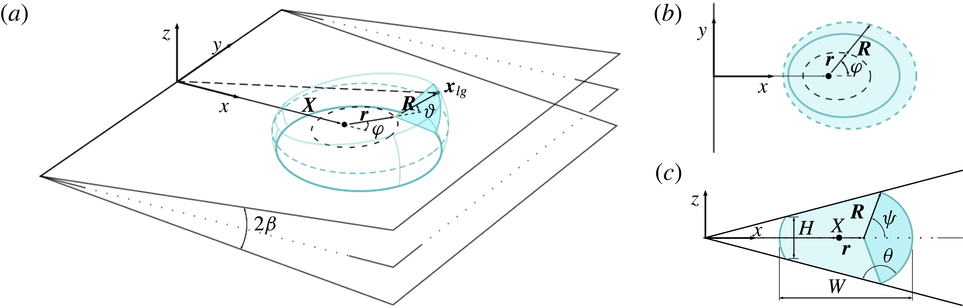
Schematics of the geometry of a liquid barrel inside a solid wedge of opening angle
 $2\unicode[STIX]{x1D6FD}$
. (a) 3-D view of the system. The position vector of the liquid–gas interface,
 $\boldsymbol{x}_{lg}$
, is described using the vectors
 $\boldsymbol{X}$
,
 $\boldsymbol{r}$
and
 $\boldsymbol{R}$
, and the azimuthal and polar angles
 $\unicode[STIX]{x1D711}$
and
 $\unicode[STIX]{x1D717}$
. (b) View of the barrel’s cross-section along the bisector plane,
 $z=0$
. The short-dashed line corresponds to the equator of the barrel. The solid line corresponds to the contact lines. (c) View of the barrel’s cross-section along the transverse plane,
 $y=0$
. The intersection with the solid occurs at a contact angle
 $\unicode[STIX]{x1D703}$
. The aspect ratio of the transverse cross-section of the barrel is determined by its minimum thickness,
 $H$
, and equatorial width,
 $W$
.

Figure 2 shows a schematic of the system under consideration, which consists of a liquid droplet that partially wets the inner surface of a wedge formed by two solid planes. We focus on a situation where the mass,
 $M$
, temperature,
 $T$
, and volume of the liquid,
 $V$
, are constant. The relevant thermodynamic potential is the Helmholtz free energy
 ${\mathcal{F}}=U-TS$
, where
 $U$
and
 $S$
are the internal energy and entropy, respectively.
From the second law of thermodynamics, the Helmholtz free energy will either remain constant or decrease upon a change in the configuration of the system, i.e.
 $\unicode[STIX]{x1D6FF}{\mathcal{F}}\leqslant 0$
. Such changes in the free energy are caused by the interfacial variations
 $$\begin{eqnarray}\text{d}F=\unicode[STIX]{x1D6FE}\text{d}A_{lg}+\unicode[STIX]{x1D6FE}_{sl}\text{d}A_{sl}+\unicode[STIX]{x1D6FE}_{sg}\text{d}A_{sg},\end{eqnarray}$$
where
 $\unicode[STIX]{x1D6FE}$
,
 $\unicode[STIX]{x1D6FE}_{sl}$
and
 $\unicode[STIX]{x1D6FE}_{sg}$
are the liquid–gas, solid–liquid and solid–gas surface tensions respectively; and
 $A_{lg}$
,
 $A_{sl}$
and
 $A_{sg}$
are the corresponding interfacial areas. Therefore, equilibrium states correspond to minima of the surface energy
 $$\begin{eqnarray}F=\unicode[STIX]{x1D6FE}(A_{lg}-A_{sl}\cos \unicode[STIX]{x1D703}_{e}),\end{eqnarray}$$
where the equilibrium angle,
 $\unicode[STIX]{x1D703}_{e}$
, is determined by Young’s law,
 $$\begin{eqnarray}\cos \unicode[STIX]{x1D703}_{e}=\frac{\unicode[STIX]{x1D6FE}_{sg}-\unicode[STIX]{x1D6FE}_{sl}}{\unicode[STIX]{x1D6FE}}.\end{eqnarray}$$
2.1 Geometry
To determine
 $F$
, we need to specify a suitable parametrisation of the geometry of the droplet, as shown in figure 2. In Cartesian coordinates, the wedge walls are oriented at an angle
 $\unicode[STIX]{x1D6FD}$
from the
 $xy$
plane and intersect along the
 $y$
axis. The unit normals to the walls are
 $\pm \hat{\boldsymbol{n}}(\pm \unicode[STIX]{x1D6FD})$
, where
 $\hat{\boldsymbol{n}}(\unicode[STIX]{x1D6FD})=(-\sin \unicode[STIX]{x1D6FD},0,\cos \unicode[STIX]{x1D6FD})$
.
We assume that the wedge walls are identical and perfectly uniform. Furthermore, we assume that the droplet shape has two planes of symmetry. In the following, we refer to these as the bisector plane,
 $$\begin{eqnarray}z=0,\end{eqnarray}$$
and the transverse plane,
 $$\begin{eqnarray}y=0.\end{eqnarray}$$
The intersection of these planes defines the bisector line,
 $$\begin{eqnarray}(x,0,0),\end{eqnarray}$$
which is the principal axis of symmetry of the droplet.
We describe a point on the liquid–gas interface using the position vector
 $$\begin{eqnarray}\boldsymbol{x}_{lg}\equiv \boldsymbol{X}+\boldsymbol{r}+\boldsymbol{R}.\end{eqnarray}$$
The vector
 $\boldsymbol{X}=(X,0,0)$
defines the position of the geometric centre of the droplet,
 $X$
, relative to the apex of the wedge. The vector
 $\boldsymbol{r}=r(\unicode[STIX]{x1D711})\hat{\boldsymbol{r}}$
, where
 $\hat{\boldsymbol{r}}=(\cos \unicode[STIX]{x1D711},\sin \unicode[STIX]{x1D711},0)$
, is a displacement vector from the geometric centre of the droplet (point
 $X$
in figure 2) confined to the bisector plane. The vector
 $\boldsymbol{R}=R(\unicode[STIX]{x1D711},\unicode[STIX]{x1D717})\hat{\boldsymbol{R}}$
, where
 $\hat{\boldsymbol{R}}=(\cos \unicode[STIX]{x1D711}\cos \unicode[STIX]{x1D717},\sin \unicode[STIX]{x1D711}\cos \unicode[STIX]{x1D717},\sin \unicode[STIX]{x1D717})$
, is a displacement vector that joins the vector
 $\boldsymbol{r}$
and a point on the liquid–gas interface.
Whilst the azimuthal angle varies in the interval
 $\unicode[STIX]{x1D711}\in [0,2\unicode[STIX]{x03C0})$
, the polar angle is restricted by the intersection of the liquid–gas interface with the solid walls, i.e.
 $\unicode[STIX]{x1D717}\in [-\unicode[STIX]{x1D713},\unicode[STIX]{x1D713}]$
, where the maximum angle,
 $\unicode[STIX]{x1D713}$
, can be found by the geometrical condition
 $$\begin{eqnarray}\hat{\boldsymbol{n}}(\pm \unicode[STIX]{x1D6FD})\boldsymbol{\cdot }\boldsymbol{x}_{lg}(\unicode[STIX]{x1D711},\unicode[STIX]{x1D717}=\pm \unicode[STIX]{x1D713})=0.\end{eqnarray}$$
In addition, one can write a relation for the contact angle of the liquid–gas interface with the solid,
 $\unicode[STIX]{x1D703}$
, measured from the liquid phase, which reads
 $$\begin{eqnarray}-\cos \,\unicode[STIX]{x1D703}=\pm \hat{\boldsymbol{n}}(\pm \unicode[STIX]{x1D6FD})\boldsymbol{\cdot }\frac{\unicode[STIX]{x2202}_{\unicode[STIX]{x1D711}}\boldsymbol{x}_{lg}\times \unicode[STIX]{x2202}_{\unicode[STIX]{x1D717}}\boldsymbol{x}_{lg}}{|\unicode[STIX]{x2202}_{\unicode[STIX]{x1D711}}\boldsymbol{x}_{lg}\times \unicode[STIX]{x2202}_{\unicode[STIX]{x1D717}}\boldsymbol{x}_{lg}|}(\unicode[STIX]{x1D711},\unicode[STIX]{x1D717}=\pm \unicode[STIX]{x1D713}).\end{eqnarray}$$
The aspect ratio of the droplet can be characterised by the height-to-width ratio of the transverse cross-section,
 $$\begin{eqnarray}h\equiv \frac{H}{W},\end{eqnarray}$$
where the droplet height,
 $H\equiv |\boldsymbol{x}_{lg}(\unicode[STIX]{x03C0},\unicode[STIX]{x1D713})-\boldsymbol{x}_{lg}(\unicode[STIX]{x03C0},-\unicode[STIX]{x1D713})|,$
is the length of the line connecting the contact lines at the narrow end of the wedge and the droplet width,
 $W\equiv |\boldsymbol{x}_{lg}(0,0)-\boldsymbol{x}_{lg}(\unicode[STIX]{x03C0},0)|$
, is the distance between the leading and trailing points of the droplet’s equator.
Using the parametrisation
 $\boldsymbol{x}_{lg}(\unicode[STIX]{x1D711},\unicode[STIX]{x1D717})$
, we define the surface elements of the liquid–gas and solid–liquid interfaces as
 $$\begin{eqnarray}\displaystyle & \displaystyle \text{d}\boldsymbol{A}_{lg}\equiv (\unicode[STIX]{x2202}_{\unicode[STIX]{x1D711}}\boldsymbol{x}_{lg}\times \unicode[STIX]{x2202}_{\unicode[STIX]{x1D717}}\boldsymbol{x}_{lg})\,\text{d}\unicode[STIX]{x1D717}\,\text{d}\unicode[STIX]{x1D711}, & \displaystyle\end{eqnarray}$$
 $$\begin{eqnarray}\displaystyle & \displaystyle \text{d}\boldsymbol{A}_{sl}\equiv \frac{1}{2}\boldsymbol{x}_{lg}(\unicode[STIX]{x1D711},\unicode[STIX]{x1D713})\times \frac{\text{d}}{\text{d}\unicode[STIX]{x1D711}}\boldsymbol{x}_{lg}(\unicode[STIX]{x1D711},\unicode[STIX]{x1D713})\,\text{d}\unicode[STIX]{x1D711}. & \displaystyle\end{eqnarray}$$
Therefore, the surface energy,
 $F$
, and the volume of the droplet,
 $V$
, can be expressed as
 $$\begin{eqnarray}F=\unicode[STIX]{x1D6FE}\int _{0}^{2\unicode[STIX]{x03C0}}\int _{-\unicode[STIX]{x1D713}}^{\unicode[STIX]{x1D713}}|\text{d}\boldsymbol{A}_{lg}|-2\unicode[STIX]{x1D6FE}\cos \unicode[STIX]{x1D703}_{e}\int _{0}^{2\unicode[STIX]{x03C0}}\hat{\boldsymbol{n}}\boldsymbol{\cdot }\text{d}\boldsymbol{A}_{sl},\end{eqnarray}$$
and
 $$\begin{eqnarray}V=\frac{1}{3}\int _{liq.}\unicode[STIX]{x1D735}\boldsymbol{\cdot }(x,y,z)\,\text{d}x\,\text{d}y\,\text{d}z=\frac{1}{3}\int _{0}^{2\unicode[STIX]{x03C0}}\int _{-\unicode[STIX]{x1D713}}^{\unicode[STIX]{x1D713}}\boldsymbol{x}_{lg}\boldsymbol{\cdot }\,\text{d}\boldsymbol{A}_{lg},\end{eqnarray}$$
where we have made use of the divergence theorem in the last equality.
2.2 Morphology of liquid barrels
In this section we discuss the morphology of the liquid–gas interface in static and dynamic situations close to thermodynamic equilibrium. Static droplets correspond to a mechanical equilibrium situation, where capillary forces are balanced by an external force, such as gravity. Dynamic situations, on the other hand, correspond to droplets undergoing a translational motion within the wedge, where the liquid is subject to inertial and frictional forces.
In the following we will restrict our discussion to droplets confined in narrow wedges, where
 $\unicode[STIX]{x1D6FD}$
is of the order of a few degrees. We consider droplets of characteristic linear size
 $V^{1/3}\approx 1~\text{mm}$
, made of liquids such as water, glycerol, or oils, for which the density
 $\unicode[STIX]{x1D70C}\approx 10^{3}~\text{kg}~\text{m}^{-3}$
, dynamic viscosity
 $\unicode[STIX]{x1D702}\approx 1~\text{mPa}~\text{s}$
, and surface tension
 $\unicode[STIX]{x1D6FE}\approx 20{-}70~\text{mN}~\text{m}^{-1}$
.
For droplets under the action of gravity, the Bond number is, therefore,
 $\mathit{Bo}\equiv \unicode[STIX]{x1D70C}gV^{2/3}/\unicode[STIX]{x1D6FE}\sim 10^{-1}$
, where
 $g=9.81~\text{m}~\text{s}^{-2}$
. For moving droplets inside a narrow wedge,
 $\unicode[STIX]{x1D6FD}\sim 1^{\circ }{-}10^{\circ }$
, experiments show that the typical speed is
 $U\sim 1~\text{mm}~\text{s}^{-1}{-}10~\text{mm}~\text{s}^{-1}$
(Reyssat Reference Reyssat2014; Ruiz-Gutiérrez et al.
Reference Ruiz-Gutiérrez, Guan, Xu, Mchale, Wells and Ledesma-Aguilar2017). Hence, the Reynolds number
 $\mathit{Re}\equiv \unicode[STIX]{x1D70C}UV^{1/3}\unicode[STIX]{x1D6FD}/\unicode[STIX]{x1D702}\sim 10^{-1}{-}10^{0}$
, the capillary number,
 $\mathit{Ca}\equiv \unicode[STIX]{x1D702}U/\unicode[STIX]{x1D6FE}\sim 10^{-5}{-}10^{-3}$
, and the Weber number,
 $\mathit{We}\equiv \mathit{Re}\mathit{Ca}\sim 10^{-6}{-}10^{-3}$
.
The smallness of the Reynolds number implies that inertial effects are negligible relative to viscous stresses. On the other hand, the smallness of the Weber number indicates that short-wavelength perturbations to the liquid–gas interface decay over a short time scale relative to the time scale of translational motion of the drop (Miller & Scriven Reference Miller and Scriven1968; Zhong-Can & Helfrich Reference Zhong-Can and Helfrich1987). Finally, the smallness of the Bond and capillary numbers implies that the shape of the interface is dominated by surface tension.
Therefore, we describe the near-equilibrium shape of the liquid–gas interface as a smooth barrel shape intersecting the solid at the equilibrium contact angle. In terms of the parametrisation presented in § 2.1, this corresponds to introducing the following approximations:
 $$\begin{eqnarray}\displaystyle & \unicode[STIX]{x1D703}=\unicode[STIX]{x1D703}_{e}, & \displaystyle\end{eqnarray}$$
 $$\begin{eqnarray}\displaystyle & R=R(\unicode[STIX]{x1D711}), & \displaystyle\end{eqnarray}$$
 $$\begin{eqnarray}\displaystyle & W/2=R+r=\text{const.}, & \displaystyle\end{eqnarray}$$
where
 $R(\unicode[STIX]{x1D711})$
is the radius of curvature of the interface normal to the bisector plane and
 $W/2$
is the radius of curvature of the barrel’s equator.
To obtain an explicit expression of the barrel shape, we need to substitute the assumptions (2.15)–(2.17) into (2.7)–(2.9). First, we note that under these assumptions the unit vector
 $\hat{\boldsymbol{R}}$
is approximately normal to the contact line. Therefore, the boundary condition (2.9) can be relaxed to the constraint
 $$\begin{eqnarray}-\cos \,\unicode[STIX]{x1D703}_{e}=\hat{\boldsymbol{n}}(\unicode[STIX]{x1D6FD})\boldsymbol{\cdot }\hat{\boldsymbol{R}}(\unicode[STIX]{x1D717}=\unicode[STIX]{x1D713}).\end{eqnarray}$$
This simplification leads to the following expression for the transverse radius of curvature,
 $$\begin{eqnarray}\displaystyle R(\unicode[STIX]{x1D711})=q\left(1+\unicode[STIX]{x1D716}\frac{\cos \unicode[STIX]{x1D711}}{\cos \unicode[STIX]{x1D711}-\cos \unicode[STIX]{x1D703}_{e}/\sin \unicode[STIX]{x1D6FD}}\right), & & \displaystyle\end{eqnarray}$$
where
 $$\begin{eqnarray}q\equiv -\frac{\sin \unicode[STIX]{x1D6FD}}{\cos \unicode[STIX]{x1D703}_{e}}X,\end{eqnarray}$$
and
 $$\begin{eqnarray}\unicode[STIX]{x1D716}\equiv \frac{W}{2q}-1.\end{eqnarray}$$
Here,
 $q$
is a rescaled position of the geometric centre of the barrel. Setting
 $\unicode[STIX]{x1D716}=0$
in (2.19) gives
 $R=\text{const.}$
, and thus the barrel takes the shape of a sphere truncated by the solid planes. Therefore,
 $\unicode[STIX]{x1D716}$
controls the amplitude of azimuthal distortions to the spherical shape.
For a given volume, choosing the position of the barrel fixes its equatorial width, and consequently,
 $q$
and
 $\unicode[STIX]{x1D716}$
are not independent. Rather, evaluating (2.14) gives the relation
 $$\begin{eqnarray}V(q,\unicode[STIX]{x1D716})=q^{3}\mathop{\sum }_{i=0}^{3}a_{i}\unicode[STIX]{x1D716}^{i},\end{eqnarray}$$
where the constants
 $a_{i}$
are functions of
 $\unicode[STIX]{x1D6FD}$
and
 $\unicode[STIX]{x1D703}_{e}$
, and are reported in appendix A. Their expressions, however, simplify considerably in the limit of small wedge angles. Therefore,
 $$\begin{eqnarray}\displaystyle & \displaystyle a_{0}=\frac{\unicode[STIX]{x03C0}}{6}(\cos 3\unicode[STIX]{x1D703}_{e}-9\cos \unicode[STIX]{x1D703}_{e}), & \displaystyle\end{eqnarray}$$
 $$\begin{eqnarray}\displaystyle & \displaystyle a_{1}=\unicode[STIX]{x03C0}(2\unicode[STIX]{x1D703}_{e}-\unicode[STIX]{x03C0}-\sin 2\unicode[STIX]{x1D703}_{e})+O(\unicode[STIX]{x1D6FD}^{2}), & \displaystyle\end{eqnarray}$$
 $$\begin{eqnarray}\displaystyle & \displaystyle a_{2}=-2\unicode[STIX]{x03C0}\cos \unicode[STIX]{x1D703}_{e}+O(\unicode[STIX]{x1D6FD}^{2}), & \displaystyle\end{eqnarray}$$
 $$\begin{eqnarray}\displaystyle & \displaystyle a_{3}=0+O(\unicode[STIX]{x1D6FD}^{2}). & \displaystyle\end{eqnarray}$$
Using this approximation, and inverting (2.22), we find
 $$\begin{eqnarray}\unicode[STIX]{x1D716}(q)=\frac{1}{2a_{2}}\left(\left\{a_{1}^{2}+4a_{2}\left(\frac{V}{q^{3}}-a_{0}\right)\right\}^{1/2}-a_{1}\right).\end{eqnarray}$$
2.3 Equilibrium
We first analyse the equilibrium shapes of liquid barrels in wedge geometries. Concus et al. (Reference Concus, Finn and McCuan2001) proved the existence of equilibrium states in the range
 $\unicode[STIX]{x1D703}_{e}-\unicode[STIX]{x1D6FD}>90^{\circ }$
, corresponding to sections of spheres intersecting the walls of the wedge with the equilibrium angle
 $\unicode[STIX]{x1D703}_{e}$
. Baratian et al. (Reference Baratian, Cavalli, van den Ende and Mugele2015) showed that for such solutions the surface tension acting on the wall integrated over the contact line exactly matches the pressure exerted by the liquid integrated over the solid–liquid interface.
In terms of (2.15)–(2.17), such force-free spherical shapes can be recovered by setting
 $r=0$
and
 $R=R_{e}$
, where
 $$\begin{eqnarray}\displaystyle R_{e}=\left[\frac{6V}{\unicode[STIX]{x03C0}(\cos 3\unicode[STIX]{x1D703}_{e}-9\cos \unicode[STIX]{x1D703}_{e})}\right]^{1/3}. & & \displaystyle\end{eqnarray}$$
This yields the following relations for the equilibrium position,
 $X_{e}$
, height-to-width ratio,
 $h_{e}$
, and surface energy,
 $F_{e}$
:
 $$\begin{eqnarray}\displaystyle & \displaystyle X_{e}=-\frac{\cos \unicode[STIX]{x1D703}_{e}}{\sin \unicode[STIX]{x1D6FD}}R_{e}, & \displaystyle\end{eqnarray}$$
 $$\begin{eqnarray}\displaystyle & \displaystyle h_{e}=-\cos (\unicode[STIX]{x1D703}_{e}-\unicode[STIX]{x1D6FD}), & \displaystyle\end{eqnarray}$$
 $$\begin{eqnarray}\displaystyle & \displaystyle F_{e}=\unicode[STIX]{x1D6FE}\frac{\unicode[STIX]{x03C0}}{3}(\cos 3\unicode[STIX]{x1D703}_{e}-9\cos \unicode[STIX]{x1D703}_{e})R_{e}^{2}, & \displaystyle\end{eqnarray}$$
while the equilibrium rescaled variables read
 $$\begin{eqnarray}\displaystyle & q_{e}=R_{e}, & \displaystyle\end{eqnarray}$$
 $$\begin{eqnarray}\displaystyle & \unicode[STIX]{x1D716}_{e}=0. & \displaystyle\end{eqnarray}$$
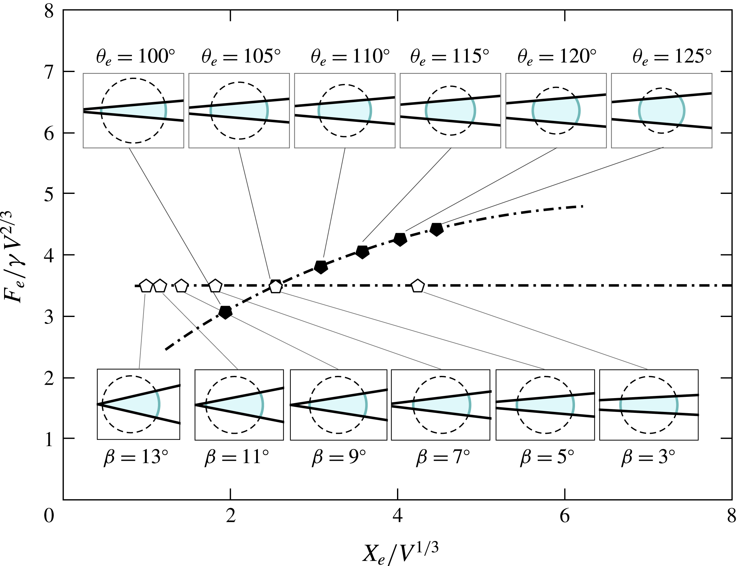
Figure 3 shows the equilibrium surface energy of liquid barrels at different positions within the wedge. We first focus on the effect of
 $\unicode[STIX]{x1D703}_{e}$
on
 $F_{e}$
and
 $X_{e}$
. For
 $\unicode[STIX]{x1D703}_{e}<180^{\circ }$
, a suspended droplet will always reduce the total surface energy by wetting the walls of the wedge. This wetted area is larger for smaller
 $\unicode[STIX]{x1D703}_{e}$
, and, because of volume conservation, the liquid settles at an equilibrium position closer to the wedge apex (see insets in figure 3). At first sight, one might expect a similar effect by increasing the wedge angle,
 $\unicode[STIX]{x1D6FD}$
. Indeed, from (2.29), an increase in the wedge angle leads to a closer position of the barrel to the wedge apex. The surface energy, however, remains constant. Geometrically, this can be understood by noting that a change in
 $\unicode[STIX]{x1D6FD}$
is equivalent to a rotation of the excluded portions of the truncated sphere (shown as dashed lines in the insets of figure 3) about the centre of the sphere, which does not alter the size of any of the interfaces of the barrel.
Equilibrium surface energy,
 $F_{e}$
, as a function of the distance from the wedge apex,
 $X_{e}$
, for different equilibrium contact angles at fixed
 $\unicode[STIX]{x1D6FD}=5^{\circ }$
(full symbols) and wedge angles at fixed
 $\unicode[STIX]{x1D703}_{e}=105^{\circ }$
(empty symbols). The insets correspond to cross-sections of the barrels along the transverse plane.

Note that for the droplet to form a closed barrel, that is, a structure that bridges the walls of the wedge avoiding its apex, one must have
 $R_{e}<X_{e}$
, or, equivalently,
 $$\begin{eqnarray}h_{e}>0.\end{eqnarray}$$
From (2.30), this condition is satisfied only if
 $$\begin{eqnarray}\unicode[STIX]{x1D703}_{e}-\unicode[STIX]{x1D6FD}>90^{\circ }.\end{eqnarray}$$
Equilibrium states can also exist if
 $\unicode[STIX]{x1D703}_{e}-\unicode[STIX]{x1D6FD}\leqslant 90^{\circ }$
, but not as liquid barrel shapes. In such cases it has been shown that the liquid completely invades the wedge (Reyssat Reference Reyssat2014) and forms edge blobs (Concus & Finn Reference Concus and Finn1998; Concus et al.
Reference Concus, Finn and McCuan2001) or filaments that spread laterally along the wedge apex (Brinkmann & Blossey Reference Brinkmann and Blossey2004).
For a parallel-plate geometry (
 $\unicode[STIX]{x1D6FD}=0^{\circ }$
), force-free barrels can exist provided that the separation between the solid walls matches the equilibrium height
 $$\begin{eqnarray}H_{e}=2h_{e}R_{e},\end{eqnarray}$$
which follows easily from (2.30). As noted by Kusumaatmaja & Lipowsky (Reference Kusumaatmaja and Lipowsky2010), a displacement of the solid wall from this equilibrium configuration will still result in mechanical equilibrium, albeit in the presence of a net external force. This situation can also occur for capillary bridges (
 $\unicode[STIX]{x1D703}_{e}<90^{\circ }-\unicode[STIX]{x1D6FD}$
), for which no force-free equilibrium configurations can exist and the net force exerted by the liquid on the solid plates is always attractive.
2.4 Energy landscapes
We now focus on the energy change due to a small change in the position of the barrel from equilibrium, corresponding to
 $\unicode[STIX]{x1D716}\ll 1$
. Therefore, we express the free energy
 $F$
(2.13) as a polynomial expansion in
 $\unicode[STIX]{x1D716}$
. After some manipulations, we obtain
 $$\begin{eqnarray}F(q,\unicode[STIX]{x1D716})=\unicode[STIX]{x1D6FE}q^{2}\mathop{\sum }_{i=0}^{3}(3-i)a_{i}\unicode[STIX]{x1D716}^{i}+O(\unicode[STIX]{x1D716}^{4}).\end{eqnarray}$$
The constant-volume energy landscapes,
 $F_{V}(X)$
, are then obtained by inserting (2.27) into (2.37) and recovering the definition of
 $q$
from (2.20), i.e.
 $$\begin{eqnarray}F_{V}(X)\equiv F\circ \unicode[STIX]{x1D716}\circ q(X).\end{eqnarray}$$
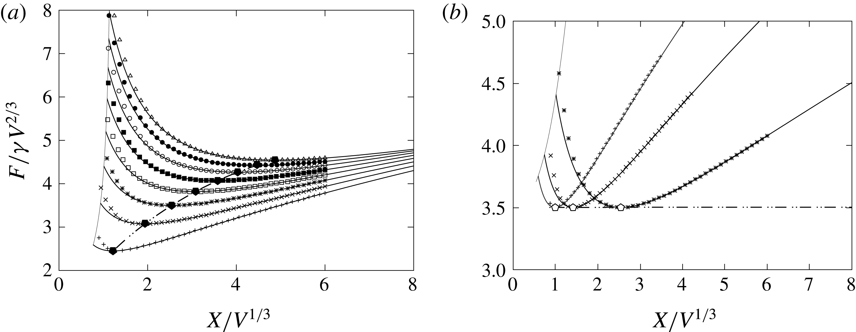
Figure 4(a) shows the energy landscapes for several values of
 $\unicode[STIX]{x1D703}_{e}$
but keeping
 $\unicode[STIX]{x1D6FD}=5^{\circ }$
. The asymmetry in the landscapes about the equilibrium position arises from the intrinsic asymmetry of the geometry of the wedge. A displacement towards the apex of the wedge induces a comparatively larger increase in the solid–liquid surface area relative to the liquid–gas surface area, and results in a sharper increase in the surface energy. This same feature is observed in figure 4(b), where we present energy landscapes at fixed
 $\unicode[STIX]{x1D703}_{e}=105^{\circ }$
and different values of
 $\unicode[STIX]{x1D6FD}$
.
Energy landscapes along the position of the liquid barrel within the wedge,
 $X$
, calculated analytically (solid lines) and numerically via constrained minimisation of the surface energy (symbols). (a) Curves for fixed
 $\unicode[STIX]{x1D6FD}=5^{\circ }$
and different equilibrium contact angles:
 $\unicode[STIX]{x1D703}_{e}=95^{\circ }$
(
 $+$
),
 $\unicode[STIX]{x1D703}_{e}=100^{\circ }$
(
 $\times$
),
 $\unicode[STIX]{x1D703}_{e}=105^{\circ }$
(*),
 $\unicode[STIX]{x1D703}_{e}=110^{\circ }$
(▫),
 $\unicode[STIX]{x1D703}_{e}=115^{\circ }$
(▪),
 $\unicode[STIX]{x1D703}_{e}=120^{\circ }$
(○),
 $\unicode[STIX]{x1D703}_{e}=125^{\circ }$
(●), and
 $\unicode[STIX]{x1D703}_{e}=130^{\circ }$
(▵). (b) Curves for fixed
 $\unicode[STIX]{x1D703}_{e}=105^{\circ }$
and different wedge angles:
 $\unicode[STIX]{x1D6FD}=5^{\circ }$
(*),
 $\unicode[STIX]{x1D6FD}=9^{\circ }$
(
 $\times$
) and
 $\unicode[STIX]{x1D6FD}=13^{\circ }$
(
 $+$
). The pentagons correspond to the minima in the analytical curves. The solid cutoff lines correspond to the limit where the liquid–gas interface touches the apex of the wedge.

2.5 Pressure distribution
In the limit of small Reynolds and Weber numbers, the local conservation of momentum within the liquid is governed by the Stokes equations
 $$\begin{eqnarray}0=-\unicode[STIX]{x1D735}p+\unicode[STIX]{x1D702}\unicode[STIX]{x1D6FB}^{2}\boldsymbol{u}+\unicode[STIX]{x1D70C}\boldsymbol{g},\end{eqnarray}$$
where
 $p$
is the pressure field,
 $\boldsymbol{u}$
is the velocity field, and
 $\unicode[STIX]{x1D70C}\boldsymbol{g}$
is the body force density exerted by gravity. For an incompressible fluid, the continuity equation reduces to the incompressibility condition
 $$\begin{eqnarray}\unicode[STIX]{x1D735}\boldsymbol{\cdot }\boldsymbol{u}=0.\end{eqnarray}$$
The model for the barrel shape presented in § 2.2 provides a means to calculate the pressure distribution within the liquid in both static and dynamic situations. Specifically, combining equations (2.39) and (2.40) to eliminate
 $\boldsymbol{u}$
and
 $\unicode[STIX]{x1D70C}\boldsymbol{g}$
(Pozrikidis Reference Pozrikidis1992; Landau & Lifshitz Reference Landau and Lifshitz2013) leads to the result that the pressure satisfies Laplace’s equation,
 $$\begin{eqnarray}\unicode[STIX]{x1D6FB}^{2}p=0.\end{eqnarray}$$
Here, the geometry of the wedge and the configuration of the barrel provide the boundary conditions for
 $p$
. At the solid walls, we impose the impenetrability condition
 $$\begin{eqnarray}\hat{\boldsymbol{n}}\boldsymbol{\cdot }\unicode[STIX]{x1D735}p(\boldsymbol{x}_{sl})=0.\end{eqnarray}$$
At the liquid–gas interface, on the other hand, the pressure is determined by the local barrel shape via the Young–Laplace law,
 $$\begin{eqnarray}p(\boldsymbol{x}_{lg})=2\unicode[STIX]{x1D6FE}\unicode[STIX]{x1D705},\end{eqnarray}$$
where
 $\unicode[STIX]{x1D705}$
is the mean curvature of the interface.
To determine the pressure profile we need to solve the boundary value problem posed by (2.41)–(2.43). The mean curvature,
 $\unicode[STIX]{x1D705}$
, follows from (2.18)–(2.21). The calculation is simplified significantly using toroidal coordinates, as reported in detail in appendix B. Having determined the mean curvature, we solve Laplace’s equation using separation of variables and express the solution as a harmonic series. The calculation is lengthy, and we thus refer the reader to appendix C for details.
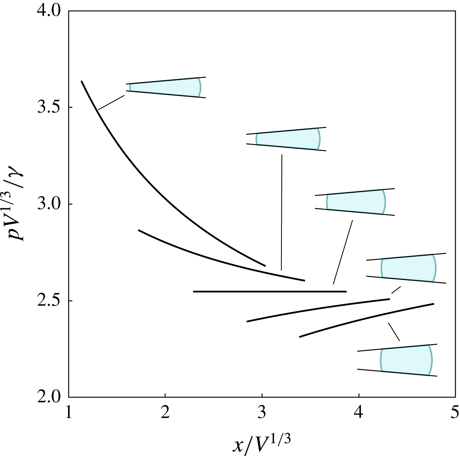
Pressure profiles along the bisector line
 $(x,0,0)$
for out-of-equilibrium barrel shapes of equilibrium contact angle
 $\unicode[STIX]{x1D703}_{e}=110^{\circ }$
and wedge angle
 $\unicode[STIX]{x1D6FD}=5^{\circ }$
(shown as insets). Each of the curves corresponds to a different displacement from equilibrium. From left to right,
 $(X-X_{e})/V^{1/3}=-1,-1/2,0,1/2,1$
.

To illustrate our result, let us first consider the mean curvature at the equator of the barrel, which reads
 $$\begin{eqnarray}\unicode[STIX]{x1D705}(\unicode[STIX]{x1D711},\unicode[STIX]{x1D717}=0)=\frac{1}{W}+\frac{1}{2R(\unicode[STIX]{x1D711})}=\frac{1}{2q}\left(1+\frac{1}{1+\unicode[STIX]{x1D716}}+\frac{\unicode[STIX]{x1D716}\sin \unicode[STIX]{x1D6FD}\cos \unicode[STIX]{x1D711}}{(1+\unicode[STIX]{x1D716})\sin \unicode[STIX]{x1D6FD}\cos \unicode[STIX]{x1D711}-\cos \unicode[STIX]{x1D703}_{e}}\right).\end{eqnarray}$$
Evaluating (2.44) at the points
 $\unicode[STIX]{x1D711}=0$
and
 $\unicode[STIX]{x1D711}=\unicode[STIX]{x03C0}$
leads to an expression for the Laplace pressure drop along the bisector line, which reads
 $$\begin{eqnarray}\unicode[STIX]{x0394}p=-\frac{8\unicode[STIX]{x1D6FE}X\unicode[STIX]{x1D716}}{4X^{2}-W^{2}}.\end{eqnarray}$$
Equation (2.45) gives an indication of the structure of the pressure profiles along the bisector line, which we present in figure 5. We first note that geometry dictates that
 $X>W/2$
. Therefore, the sign of
 $\unicode[STIX]{x0394}p$
is controlled by
 $\unicode[STIX]{x1D716}$
. Inwards displacements, corresponding to
 $\unicode[STIX]{x1D716}>0$
, give
 $\unicode[STIX]{x0394}p<0$
, indicating that the barrel is subject to an outwards force due to the pressure gradient. The converse situation occurs for
 $\unicode[STIX]{x1D716}<0$
. The magnitude of
 $\unicode[STIX]{x0394}p$
increases as
 $X\rightarrow W/2$
, reflecting the stronger effect of confinement for inwards displacements from the equilibrium position. In equilibrium, where
 $\unicode[STIX]{x1D716}=0$
, the pressure profile is uniform (
 $\unicode[STIX]{x0394}p=0$
), and corresponds to
 $p(x,y=0,z=0)=2\unicode[STIX]{x1D6FE}/R_{e}$
, as expected for a spherical barrel shape.
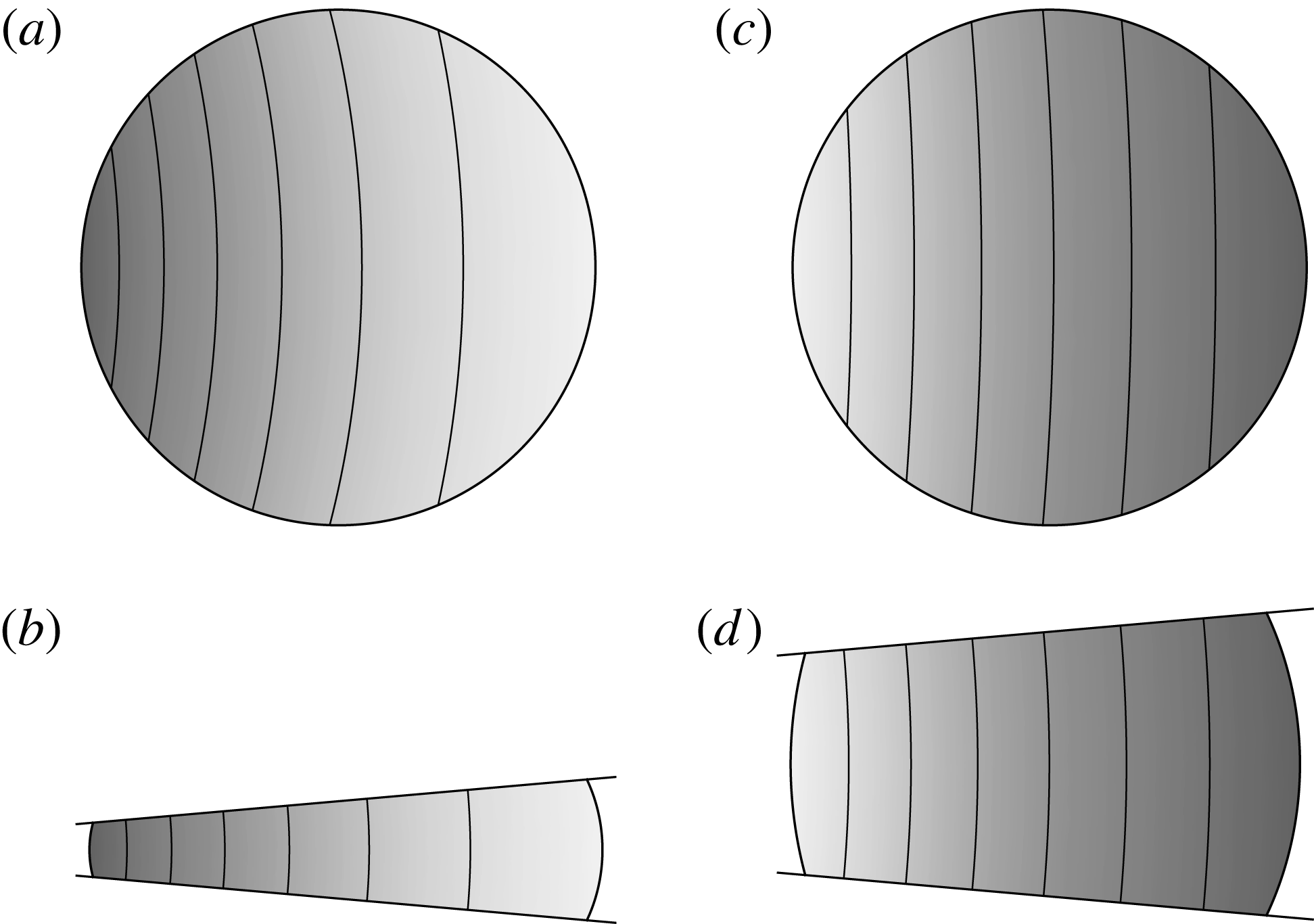
Pressure field,
 $p(\boldsymbol{x})$
, for a barrel displaced inwards (a,b), and outwards (c,d), from the equilibrium position. In each panel, a darker shading indicates a higher pressure. (a,c) Projections of the pressure field on the equatorial plane,
 $z=0$
. (b,d) Projections on the transverse plane,
 $y=0$
. The displacement in (a,b) is
 $(X-X_{e})/V^{1/3}=-1$
, and in (c,d),
 $(X-X_{e})/V^{1/3}=+1$
. The contact and tapering angles are
 $\unicode[STIX]{x1D703}_{e}=110^{\circ }$
and
 $\unicode[STIX]{x1D6FD}=5^{\circ }$
.

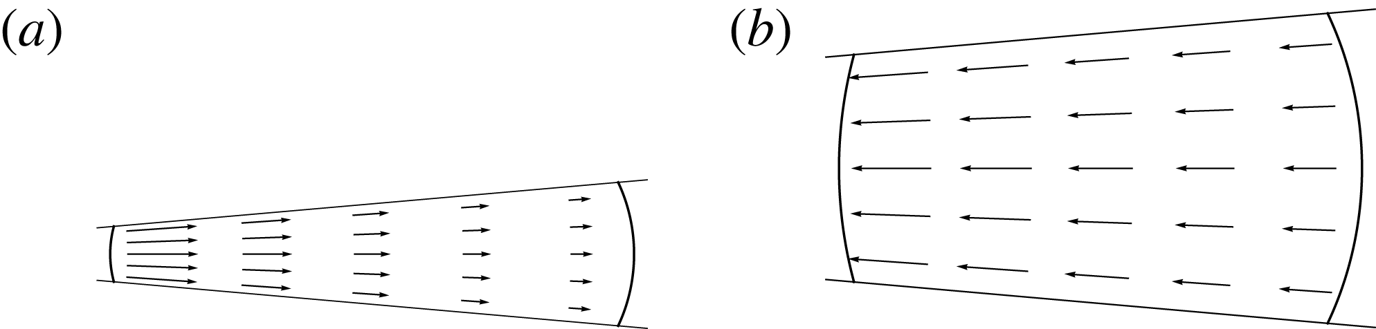
Pressure gradient force density,
 $-\unicode[STIX]{x1D735}p$
, for a barrel displaced (a) inwards and (b) outwards from the equilibrium position. The plots correspond to cross-sections along the transverse plane,
 $y=0$
. The displacements in (a,b) correspond to
 $X-X_{e}=-V^{1/3}$
and
 $X-X_{e}=+V^{1/3}$
. The contact and tapering angles are
 $\unicode[STIX]{x1D703}_{e}=110^{\circ }$
and
 $\unicode[STIX]{x1D6FD}=5^{\circ }$
.

As shown in the contour plots of figure 6, the 3-D pressure distribution broadly follows the same structure as the pressure profile along the bisector line. For barrels displaced inwards and outwards from their equilibrium position, the contour lines of the pressure field are denser towards the narrow end of the barrel, implying a stronger capillary force caused by the effect of confinement. This is confirmed by inspection of the pressure gradient force density,
 $-\unicode[STIX]{x1D735}p$
, shown in figure 7, which is radial and decreases in magnitude with increasing distance from the apex of the wedge.
3 Statics: comparison to liquid barrels deformed by gravity
The pressure profiles shown in figure 5 suggest that the out-of-equilibrium barrel morphologies presented in § 2.2 capture the effect of a uniform force density, such as gravity, on the shape of the liquid–gas interface.
To verify this hypothesis, we employed a finite element approach to numerically compute the barrel morphologies in mechanical equilibrium subject to a constraint in the position of the centre of mass. To this aim we used the public domain software SURFACE EVOLVER (Brakke Reference Brakke1992) to define a triangulated mesh describing the liquid surface and to minimise the surface energy through a conjugate gradient algorithm.
In the numerical method, the Lagrange multiplier of the volume constraint,
 $\unicode[STIX]{x1D706}_{V}$
, plays the role of the Laplace pressure at the coordinate
 $x=0$
, while the Lagrange multiplier of the centre of mass,
 $\unicode[STIX]{x1D706}_{X}$
, can be interpreted as an effective body force required to hold the droplet in place. Therefore, a linear hydrostatic pressure profile can be constructed by writing
 $p_{hs}(x)=\unicode[STIX]{x1D706}_{V}+\unicode[STIX]{x1D706}_{X}V^{2/3}x/\unicode[STIX]{x1D6FE}$
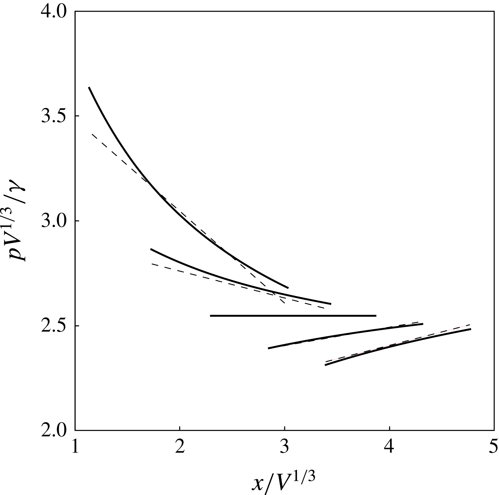
. In figure 8 we overlay the linear pressure profiles obtained numerically to the analytical curves. The range of each curve corresponds to the equatorial width of the barrel in each model. As expected, there is good agreement in the magnitude of the pressure and in the location of the edges close to equilibrium with the analytical model, particularly for
 $X>X_{e}$
. This agreement is also observed when comparing the analytical and numerical energy landscapes, as shown in figure 4(a,b).
Comparison of the pressure profiles along the bisector line for out-of-equilibrium barrel shapes obtained analytically (solid lines) to hydrostatic profiles obtained via constrained free-energy minimisation (dashed lines). From left to right, the curves correspond to the set of displacements
 $(X-X_{e})/V^{1/3}=-1,-1/2,0,1/2,1$
. The equilibrium and wedge angles are
 $\unicode[STIX]{x1D703}_{e}=110^{\circ }$
and
 $\unicode[STIX]{x1D6FD}=5^{\circ }$
.

In order to quantify the deviations between the pressure profile of the barrel and the linear hydrostatic pressure profile we consider the limit of small displacements from equilibrium. In such a case, the hydrostatic pressure profile increasingly approaches the Laplace pressure profile within the droplet, i.e.
 $$\begin{eqnarray}p_{hs}(x)\simeq 2\unicode[STIX]{x1D6FE}\unicode[STIX]{x1D705}(\unicode[STIX]{x03C0},0)+\frac{\unicode[STIX]{x0394}p}{W}(x-X+W/2).\end{eqnarray}$$
Therefore, a measure of the deviations between
 $p$
and
 $p_{hs}$
is the residual pressure
 $$\begin{eqnarray}\unicode[STIX]{x1D6FF}p_{hs}\equiv [p-p_{hs}]_{\boldsymbol{x}_{lg}(\unicode[STIX]{x1D711},\unicode[STIX]{x1D717}=0)},\end{eqnarray}$$
i.e. the difference between the pressure of the barrel and the hydrostatic pressure profile at a point along the barrel’s equator. After some calculations we obtain
 $$\begin{eqnarray}\unicode[STIX]{x1D6FF}p_{hs}=\frac{4\unicode[STIX]{x1D6FE}X\unicode[STIX]{x1D716}}{W^{2}-4X^{2}}\left(\frac{W\sin ^{2}\unicode[STIX]{x1D711}}{W\cos \unicode[STIX]{x1D711}+2X}\right).\end{eqnarray}$$
For a given barrel configuration, we calculate the maximum of
 $\unicode[STIX]{x1D6FF}p_{hs}/p$
along the equator, giving the convergence criterion
 $$\begin{eqnarray}\max \left|\frac{\unicode[STIX]{x1D6FF}p_{hs}}{p}\right|_{\boldsymbol{x}_{lg}(\unicode[STIX]{x1D711},\unicode[STIX]{x1D717}=0)}\approx \frac{1}{2}\left(\frac{R_{e}}{X_{e}}\right)^{2}|\unicode[STIX]{x1D716}|\ll 1.\end{eqnarray}$$
The dependence on
 $\unicode[STIX]{x1D716}$
shows that the barrel shape is a good approximation of the gravity-deformed droplets close to equilibrium. For a given translational displacement from equilibrium, distortions are stronger for inwards displacements due to the dependence of
 $\unicode[STIX]{x1D716}$
on
 $X$
(2.27), and for barrels initially closer to the apex of the wedge due to the effect of confinement, as indicated by the dependence on
 $R_{e}/X_{e}$
.
4 Dynamics: motion of a liquid barrel near equilibrium
4.1 Lagrangian formulation
The barrel morphologies obtained in § 2.4 correspond to a translational displacement of the liquid along the bisector line. Here we analyse the relaxation of the position of the barrel,
 $X(t)$
, back to the equilibrium position,
 $X_{e}$
. The advantage of the free-energy model is to provide an expression of the net capillary force,
 $-\text{d}F_{V}/\text{d}X$
, that drives such a relaxation. For slow motions, corresponding to the overdamped regime, the driving force acting on the barrel will be balanced by a friction force. This will depend on the viscous stresses within the liquid and on the contact-line friction offered by the solid walls. Therefore, the dynamics is amenable to a coarse-grained description that focuses on the time evolution of
 $X(t)$
. In this section we derive the equations of motion at this level of description based on a Lagrangian formulation.
Consider the generic Lagrangian
 $L(\unicode[STIX]{x1D709},\dot{\unicode[STIX]{x1D709}})$
, where
 $\unicode[STIX]{x1D709}=\{\unicode[STIX]{x1D709}_{i}\}$
and
 $\dot{\unicode[STIX]{x1D709}}=\{\dot{\unicode[STIX]{x1D709}_{i}}\}$
are a set of generalised coordinates and generalised velocities. The equations of motion are obtained by writing the Euler–Lagrange equations
 $$\begin{eqnarray}\frac{\text{d}}{\text{d}t}\left(\frac{\unicode[STIX]{x2202}L}{\unicode[STIX]{x2202}\dot{\unicode[STIX]{x1D709}}_{i}}\right)-\frac{\unicode[STIX]{x2202}L}{\unicode[STIX]{x2202}\unicode[STIX]{x1D709}_{i}}=K_{i},\end{eqnarray}$$
where we have introduced the set of (non-conservative) friction forces
 $K=\{K_{i}\}$
.
For zero
 $K_{i}$
, the energy of the system,
 $$\begin{eqnarray}{\mathcal{E}}=\mathop{\sum }_{i}\dot{\unicode[STIX]{x1D709}}_{i}\frac{\unicode[STIX]{x2202}L}{\unicode[STIX]{x2202}\dot{\unicode[STIX]{x1D709}}_{i}}-L,\end{eqnarray}$$
is a conserved quantity (Goldstein, Poole & Safko Reference Goldstein, Poole and Safko2001). This situation changes for non-zero
 $K_{i}$
, where the energy is dissipated by friction at a rate (see, e.g. Galley Reference Galley2013)
 $$\begin{eqnarray}\dot{{\mathcal{E}}}=\mathop{\sum }_{i}\dot{\unicode[STIX]{x1D709}}_{i}K_{i}.\end{eqnarray}$$
In situations where the friction forces are linear functions of the velocity, i.e.
 $$\begin{eqnarray}K_{i}=-\unicode[STIX]{x1D708}_{i}\dot{\unicode[STIX]{x1D709}}_{i},\end{eqnarray}$$
where
 $\unicode[STIX]{x1D708}_{i}$
is a friction coefficient, one obtains the result
 $$\begin{eqnarray}\dot{{\mathcal{E}}}=-\mathop{\sum }_{i}\unicode[STIX]{x1D708}_{i}{\dot{\unicode[STIX]{x1D709}}_{i}}^{2},\end{eqnarray}$$
which is called a Rayleigh dissipation function (Goldstein et al.
Reference Goldstein, Poole and Safko2001). Therefore, if
 $\dot{{\mathcal{E}}}$
is known, it can be used to determine the friction coefficients; namely:
 $$\begin{eqnarray}\unicode[STIX]{x1D708}_{i}=-\frac{1}{2}\frac{\unicode[STIX]{x2202}^{2}\dot{{\mathcal{E}}}}{\unicode[STIX]{x2202}{\dot{\unicode[STIX]{x1D709}}_{i}}^{2}}.\end{eqnarray}$$
The instantaneous barrel configuration, given by (2.19), is controlled by the coordinates
 $q$
and
 $\unicode[STIX]{x1D716}$
. Hence, the Lagrangian of the system is
 $L(q,\dot{q},\unicode[STIX]{x1D716},\dot{\unicode[STIX]{x1D716}})$
, where
 $q(t)$
and
 $\unicode[STIX]{x1D716}(t)$
are treated as dynamical variables and
 $\dot{q}\equiv \text{d}q/\text{d}t$
and
 $\dot{\unicode[STIX]{x1D716}}\equiv \text{d}\unicode[STIX]{x1D716}/\text{d}t$
are the corresponding velocities. As discussed in § 2.2, we focus on the overdamped regime, where inertial effects are negligible. Therefore,
 $L$
can be written purely in terms of the surface energy,
 $F$
. Imposing the constraint of a constant volume,
 $V=V_{0}$
, gives
 $$\begin{eqnarray}L=-F+\tilde{p}(V-V_{0}),\end{eqnarray}$$
where
 $\tilde{p}$
is a Lagrange multiplier.
Inserting this expression into (4.1) and using (4.4) gives the equations of motion
 $$\begin{eqnarray}\displaystyle & \displaystyle \frac{\unicode[STIX]{x2202}F}{\unicode[STIX]{x2202}q}-\tilde{p}\frac{\unicode[STIX]{x2202}V}{\unicode[STIX]{x2202}q}=-\unicode[STIX]{x1D708}_{q}\dot{q}, & \displaystyle\end{eqnarray}$$
 $$\begin{eqnarray}\displaystyle & \displaystyle \frac{\unicode[STIX]{x2202}F}{\unicode[STIX]{x2202}\unicode[STIX]{x1D716}}-\tilde{p}\frac{\unicode[STIX]{x2202}V}{\unicode[STIX]{x2202}\unicode[STIX]{x1D716}}=-\unicode[STIX]{x1D708}_{\unicode[STIX]{x1D716}}\dot{\unicode[STIX]{x1D716}}. & \displaystyle\end{eqnarray}$$
The time evolution of the position of the barrel,
 $X(t)$
, follows from the equation of motion
 $$\begin{eqnarray}\frac{\text{d}F_{V}}{\text{d}X}=-\unicode[STIX]{x1D708}_{X}{\dot{X}},\end{eqnarray}$$
where the term in the right-hand side is obtained by differentiating (2.38). The drag coefficient
 $\unicode[STIX]{x1D708}_{X}$
can be related to
 $\unicode[STIX]{x1D708}_{q}$
and
 $\unicode[STIX]{x1D708}_{\unicode[STIX]{x1D716}}$
. Enforcing the conservation of volume explicitly gives
 $$\begin{eqnarray}\dot{V}=\frac{\unicode[STIX]{x2202}V}{\unicode[STIX]{x2202}q}\dot{q}+\frac{\unicode[STIX]{x2202}V}{\unicode[STIX]{x2202}\unicode[STIX]{x1D716}}\dot{\unicode[STIX]{x1D716}}=0.\end{eqnarray}$$
This relation can then be used in conjunction with (4.8) and (4.9) to obtain
 $$\begin{eqnarray}\unicode[STIX]{x1D708}_{X}=\left(\frac{\text{d}q}{\text{d}X}\right)^{2}\left\{\unicode[STIX]{x1D708}_{q}+\left(\frac{\text{d}\unicode[STIX]{x1D716}}{\text{d}q}\right)^{2}\unicode[STIX]{x1D708}_{\unicode[STIX]{x1D716}}\right\}.\end{eqnarray}$$
4.2 Flow patterns
In order to determine the friction coefficients introduced in § 4.1, we need to specify the dissipation function
 $\dot{{\mathcal{E}}}$
. This, in turn, depends on the details of the flow pattern within the barrel. In this section we discuss the flow pattern emerging from the barrel shape introduced in § 2.2.
The approximation of the pressure distribution within the barrel, derived in § 2.5, implies that, in the absence of external forces, the Stokes equations (2.39) can be written as
 $$\begin{eqnarray}\unicode[STIX]{x1D702}\unicode[STIX]{x1D6FB}^{2}\boldsymbol{u}=\unicode[STIX]{x1D735}p,\end{eqnarray}$$
which have been reduced to a set of partial differential equations for the components of the velocity field
 $\boldsymbol{u}$
.
Due to the linearity of the Stokes equations,
 $\boldsymbol{u}$
can be expressed as a superposition of the flow patterns in two distinct regions. These correspond to the region near the contact lines, and to the bulk region of the barrel.
We first consider the region near the contact lines. Voinov (Reference Voinov1976) and Cox (Reference Cox1986) first showed that the flow pattern in this region is generic of dynamic wetting problems (Bonn et al.
Reference Bonn, Eggers, Indekeu, Meunier and Rolley2009), and is determined by the competition between capillary and viscous forces. As shown by Snoeijer (Reference Snoeijer2006), the dominant flow pattern is a corner flow where the shape of the interface is described by the apparent contact angle of the liquid–gas interface with the solid,
 $\unicode[STIX]{x1D703}$
. In the frame of reference of the contact line, the flow field reads
 $$\begin{eqnarray}\displaystyle \boldsymbol{u}_{corner}(s,\unicode[STIX]{x1D719}) & = & \displaystyle v_{cl}\left[\frac{(\cos \unicode[STIX]{x1D719}-\unicode[STIX]{x1D719}\sin \unicode[STIX]{x1D719})\sin \unicode[STIX]{x1D703}-\unicode[STIX]{x1D703}\cos \unicode[STIX]{x1D703}\cos \unicode[STIX]{x1D719}}{\unicode[STIX]{x1D703}-\cos \unicode[STIX]{x1D703}\sin \unicode[STIX]{x1D703}}\hat{\boldsymbol{s}}\right.\nonumber\\ \displaystyle & & \displaystyle +\left.\frac{\unicode[STIX]{x1D703}\sin \unicode[STIX]{x1D719}\cos \unicode[STIX]{x1D703}-\unicode[STIX]{x1D719}\cos \unicode[STIX]{x1D719}\sin \unicode[STIX]{x1D703}}{\unicode[STIX]{x1D703}-\cos \unicode[STIX]{x1D703}\sin \unicode[STIX]{x1D703}}\hat{\unicode[STIX]{x1D753}}\right],\end{eqnarray}$$
where
 $v_{cl}$
is the speed of the contact line,
 $s$
is a radial coordinate perpendicular to the contact line and
 $\unicode[STIX]{x1D719}$
is a polar coordinate subtending from the solid wall (
 $\unicode[STIX]{x1D719}=0$
) to the liquid–gas interface (
 $\unicode[STIX]{x1D719}=\unicode[STIX]{x1D703}$
).
The main result of the Cox–Voinov theory is a relation between the shape of the interface, characterised by
 $\unicode[STIX]{x1D703}$
, and its speed
 $v_{cl}$
. This is the well-known Cox–Voinov law
 $$\begin{eqnarray}g(\unicode[STIX]{x1D703})=g(\unicode[STIX]{x1D703}_{e})+\frac{\unicode[STIX]{x1D702}v_{cl}}{\unicode[STIX]{x1D6FE}}\log \frac{\ell _{M}}{\ell _{m}},\end{eqnarray}$$
where
 $g(x)\equiv \int _{0}^{x}\text{d}x^{\prime }(x-\cos x^{\prime }\sin x^{\prime })/2\sin x^{\prime }$
. The logarithmic term in (4.15) reflects the increased viscous friction in the proximity of the contact line, where
 $\ell _{m}$
is a microscopic cutoff length scale introduced to regularise the so-called viscous dissipation singularity (Huh & Scriven Reference Huh and Scriven1971). The corner flow extends up to a macroscopic length scale,
 $\ell _{M}$
, beyond which the flow pattern is no longer generic and becomes dependent on the details of the geometry of the system.
The large-scale region corresponds to the bulk of the barrel. From the structure of the pressure field of the barrel (see figure 7), we expect that the flow pattern resembles a radial flow within a wedge geometry, also known as a Jeffery–Hamel flow (Jeffery Reference Jeffery1915; Hamel Reference Hamel1917). For a given barrel configuration, this can be written explicitly by matching the pressure drop across the barrel (2.45), to the pressure drop driving the radial flow. After some calculations, reported in detail in appendix D, we obtain
 $$\begin{eqnarray}\boldsymbol{u}_{bulk}(x,z)={\dot{X}}\frac{X}{(x^{2}+z^{2})^{1/2}}\frac{\cos 2\unicode[STIX]{x1D6FD}-\cos 2\unicode[STIX]{x1D714}}{\cos 2\unicode[STIX]{x1D6FD}-\unicode[STIX]{x1D6FD}^{-1}\sin 2\unicode[STIX]{x1D6FD}}(\cos \unicode[STIX]{x1D714}\hat{\boldsymbol{x}}+\sin \unicode[STIX]{x1D714}\hat{\boldsymbol{z}}),\end{eqnarray}$$
where
 $\unicode[STIX]{x1D714}=\arctan (z/x)$
. The corresponding pressure profile is
 $$\begin{eqnarray}p_{bulk}(x,z)=\frac{\unicode[STIX]{x1D6FE}}{W}\left(3-\frac{W\cos \unicode[STIX]{x1D703}_{e}}{2X\sin \unicode[STIX]{x1D6FD}}\right)+\frac{\unicode[STIX]{x1D6FE}}{4W}\left(1+\frac{W\cos \unicode[STIX]{x1D703}_{e}}{2X\sin \unicode[STIX]{x1D6FD}}\right)\frac{W^{2}-4X^{2}}{x^{2}+z^{2}}.\end{eqnarray}$$
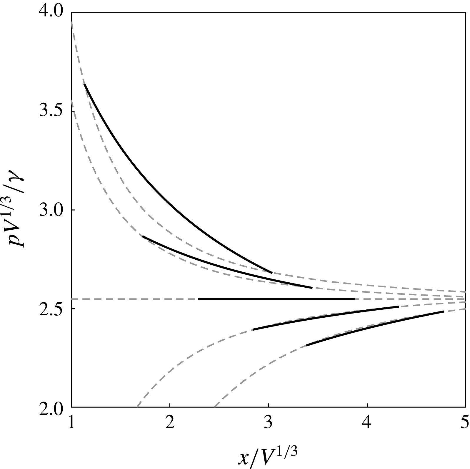
Figure 9 shows a comparison between the pressure profile of the barrel,
 $p$
, and the Jeffery–Hamel pressure profile,
 $p_{bulk}$
, along the bisector line for a set of displacements from equilibrium. There is a good match between both pressure profiles close to equilibrium. To quantify the deviations between the pressure profiles, we consider the residual pressure field along the barrel’s equator
 $$\begin{eqnarray}\unicode[STIX]{x1D6FF}p_{bulk}\equiv [p-p_{bulk}]_{\boldsymbol{x}_{lg}(\unicode[STIX]{x1D711},\unicode[STIX]{x1D717}=0)},\end{eqnarray}$$
which reads
 $$\begin{eqnarray}\unicode[STIX]{x1D6FF}p_{bulk}=\unicode[STIX]{x1D6FE}\unicode[STIX]{x1D716}\frac{W\sin ^{2}\unicode[STIX]{x1D711}}{(W\cos \unicode[STIX]{x1D711}+2X)^{2}}.\end{eqnarray}$$
Hence, the Jeffery–Hamel flow will be a good approximation of the bulk flow in the barrel provided that
 $$\begin{eqnarray}\max \left|\frac{\unicode[STIX]{x1D6FF}p_{bulk}}{p}\right|_{\boldsymbol{x}_{lg}(\unicode[STIX]{x1D711},\unicode[STIX]{x1D717}=0)}\approx \frac{1}{4}\left(\frac{R_{e}}{X_{e}}\right)^{2}\left|\unicode[STIX]{x1D716}\right|\ll 1.\end{eqnarray}$$
The meaning of this equation is that deviations grow as the barrel becomes increasingly distorted from the equilibrium shape. This is reflected in the linear dependence on
 $\unicode[STIX]{x1D716}$
. Similarly to the case of static barrels discussed in § 3, distortions are comparatively stronger for larger
 $R_{e}/X_{e}$
, i.e. for barrels increasingly confined to the apex of the wedge.
Comparison between the pressure profile of a liquid barrel along the bisector line (solid curves), to the Jeffery–Hamel pressure profile (dashed curves) for
 $\unicode[STIX]{x1D703}_{e}=120^{\circ }$
,
 $\unicode[STIX]{x1D6FD}=5^{\circ }$
and barrel positions
 $(X-X_{e})/V^{1/3}=-1,-1/2,0,+1/2,+1$
.

4.3 Sources of dissipation
Having discussed the flow pattern within the barrel, we are now in a position to derive the dissipation function
 $\dot{{\mathcal{E}}}$
. As discussed by de Gennes (Reference de Gennes1985) and de Ruijter, De Coninck & Oshanin (Reference de Ruijter, De Coninck and Oshanin1999), the total energy dissipation arising during the motion of a meniscus,
 $\dot{{\mathcal{E}}}$
, results from three main contributions,
 $$\begin{eqnarray}\dot{{\mathcal{E}}}=\dot{{\mathcal{E}}}_{{\mathcal{H}}}+\dot{{\mathcal{E}}}_{{\mathcal{L}}}+\dot{{\mathcal{E}}}_{{\mathcal{F}}},\end{eqnarray}$$
where
 $\dot{{\mathcal{E}}}_{{\mathcal{H}}}$
is the hydrodynamic dissipation,
 $\dot{{\mathcal{E}}}_{{\mathcal{L}}}$
is the dissipation due to the contact-line motion, and
 $\dot{{\mathcal{E}}}_{{\mathcal{F}}}$
is the energy dissipation arising from the formation of a precursor film ahead of the contact line. The latter term is negligible for partial wetting situations, and therefore we shall set
 $\dot{{\mathcal{E}}}_{{\mathcal{F}}}=0$
.
The hydrodynamic contribution,
 $\dot{{\mathcal{E}}}_{{\mathcal{H}}}$
, is the rate of viscous dissipation caused by the flow pattern, and reads (Landau & Lifshitz Reference Landau and Lifshitz2013),
 $$\begin{eqnarray}\dot{{\mathcal{E}}}_{{\mathcal{H}}}=-\frac{1}{2}\unicode[STIX]{x1D702}\int _{V}(\unicode[STIX]{x1D735}\boldsymbol{u}+\unicode[STIX]{x1D735}\boldsymbol{u}^{\text{T}})^{2}\,\text{d}V.\end{eqnarray}$$
Following the analysis of the flow patterns in § 4.2, the integral in (4.22) can be split into contributions coming from the bulk and corner-flow regions. i.e.
 $$\begin{eqnarray}\dot{{\mathcal{E}}}_{{\mathcal{H}}}=\dot{{\mathcal{E}}}_{bulk}+\dot{{\mathcal{E}}}_{corner}.\end{eqnarray}$$
The bulk dissipation is determined using the flow field (4.16). After some calculations, which we report in appendix E, we obtain
 $$\begin{eqnarray}\dot{{\mathcal{E}}}_{bulk}\approx -\frac{12\unicode[STIX]{x03C0}\unicode[STIX]{x1D702}X^{2}W^{2}}{\unicode[STIX]{x1D6FD}(4X^{2}-W^{2})^{3/2}}{\dot{X}}^{2}\approx -\frac{6\unicode[STIX]{x03C0}\unicode[STIX]{x1D702}}{\unicode[STIX]{x1D6FD}^{2}}|\cos \unicode[STIX]{x1D703}_{e}|(1+\unicode[STIX]{x1D716})^{2}q\dot{q}^{2}.\end{eqnarray}$$
The energy dissipation due to the corner flow near the contact line arises from a deviation of the meniscus from its equilibrium configuration. This can be quantified in terms of the apparent contact angle,
 $\unicode[STIX]{x1D703}$
. The capillary force driving the distortion of the interface is
 $$\begin{eqnarray}\boldsymbol{f}_{cl}=\unicode[STIX]{x1D6FE}(\cos \unicode[STIX]{x1D703}_{e}-\cos \unicode[STIX]{x1D703})\hat{\boldsymbol{b}}\approx \unicode[STIX]{x1D6FE}\sin \unicode[STIX]{x1D703}_{e}(\unicode[STIX]{x1D703}-\unicode[STIX]{x1D703}_{e})\hat{\boldsymbol{b}},\end{eqnarray}$$
where
 $\hat{\boldsymbol{b}}$
is the unit normal of the contact-line coplanar to the solid interface. Therefore, the energy dissipation can be expressed as (see e.g. de Gennes Reference de Gennes1985),
 $$\begin{eqnarray}\dot{{\mathcal{E}}}_{corner}=-2\oint _{cl}\boldsymbol{f}_{cl}\boldsymbol{\cdot }\boldsymbol{v}_{cl}\,\text{d}l,\end{eqnarray}$$
where the integration is over the closed loop defined by the contact line and
 $\boldsymbol{v}_{cl}=\dot{\boldsymbol{x}}_{lg}(\unicode[STIX]{x1D711},\unicode[STIX]{x1D717}=\unicode[STIX]{x1D713})$
is the velocity of the contact line.
The deviation of the dynamic contact angle from the equilibrium value can be estimated using the Cox–Voinov law (4.15), which for small
 $(\unicode[STIX]{x1D703}-\unicode[STIX]{x1D703}_{e})$
reduces to
 $$\begin{eqnarray}\frac{\unicode[STIX]{x1D703}_{e}-\cos \unicode[STIX]{x1D703}_{e}\sin \unicode[STIX]{x1D703}_{e}}{2\sin \unicode[STIX]{x1D703}_{e}}(\unicode[STIX]{x1D703}-\unicode[STIX]{x1D703}_{e})=\frac{\unicode[STIX]{x1D702}}{\unicode[STIX]{x1D6FE}}v_{cl}\log \frac{\ell _{M}}{\ell _{m}},\end{eqnarray}$$
where
 $v_{cl}=\boldsymbol{v}_{cl}\boldsymbol{\cdot }\hat{\boldsymbol{b}}$
.
Using (4.27) to eliminate
 $\unicode[STIX]{x1D703}-\unicode[STIX]{x1D703}_{e}$
from (4.26) gives
 $$\begin{eqnarray}\dot{{\mathcal{E}}}_{corner}=-\frac{4\unicode[STIX]{x1D702}\sin ^{2}\unicode[STIX]{x1D703}_{e}}{\unicode[STIX]{x1D703}_{e}-\cos \unicode[STIX]{x1D703}_{e}\sin \unicode[STIX]{x1D703}_{e}}\log \frac{\ell _{M}}{\ell _{m}}\oint _{cl}v_{cl}^{2}\,\text{d}l,\end{eqnarray}$$
where the closed-loop integral is (see appendix F for a derivation)
 $$\begin{eqnarray}\oint _{cl}v_{cl}^{2}\,\text{d}l=\frac{\unicode[STIX]{x03C0}\cos ^{2}\unicode[STIX]{x1D703}_{e}q(1+\unicode[STIX]{x1D716})\dot{q}^{2}}{\unicode[STIX]{x1D6FD}^{2}}.\end{eqnarray}$$
Finally, the contact-line dissipation,
 $\dot{{\mathcal{E}}}_{{\mathcal{L}}}$
, arises at length scales smaller than
 $\ell _{m}$
, where frictional processes are controlled by the motion of the liquid and gas molecules past the solid. Matching the average speed of the molecules to
 $v_{cl}$
one obtains the friction law (de Ruijter et al.
Reference de Ruijter, De Coninck and Oshanin1999),
 $$\begin{eqnarray}\dot{{\mathcal{E}}}_{{\mathcal{L}}}=-2\unicode[STIX]{x1D701}_{0}\oint _{cl}v_{cl}^{2}\,\text{d}l,\end{eqnarray}$$
where the friction coefficient,
 $\unicode[STIX]{x1D701}_{0}$
, is determined by the competition between the adsorption of molecules by the solid and thermal fluctuations (Blake & Haynes Reference Blake and Haynes1969).
4.4 Relaxation towards equilibrium
Close to equilibrium, the restoring force in (4.10) can be obtained by expanding
 $F_{V}$
in powers of
 $X-X_{e}$
, i.e.
 $$\begin{eqnarray}F_{V}(X)=F_{e}+{\textstyle \frac{1}{2}}k(X-X_{e})^{2}+O(X-X_{e})^{3},\end{eqnarray}$$
where the coefficient of restitution is
 $$\begin{eqnarray}k=6\unicode[STIX]{x1D6FE}a_{0}\left(1-\frac{3a_{0}a_{2}}{a_{1}^{2}}\right)\frac{\unicode[STIX]{x1D6FD}^{2}}{\cos ^{2}\unicode[STIX]{x1D703}_{e}},\end{eqnarray}$$
which, after using (2.26) reduces to
 $$\begin{eqnarray}k=\unicode[STIX]{x03C0}\unicode[STIX]{x1D6FE}\unicode[STIX]{x1D6FD}^{2}\frac{\cos 3\unicode[STIX]{x1D703}_{e}-9\cos \unicode[STIX]{x1D703}_{e}}{\cos ^{2}\unicode[STIX]{x1D703}_{e}}\left[1+\frac{2\cos ^{2}\unicode[STIX]{x1D703}_{e}(\cos 2\unicode[STIX]{x1D703}_{e}-5)}{(\unicode[STIX]{x03C0}-2\unicode[STIX]{x1D703}_{e}+\sin 2\unicode[STIX]{x1D703}_{e})^{2}}\right].\end{eqnarray}$$
To estimate the drag coefficient,
 $\unicode[STIX]{x1D708}_{X}$
, we first substitute (4.24), (4.28) and (4.30) into (4.21). Then, using (4.6), gives, to leading order in
 $\unicode[STIX]{x1D6FD}$
,
 $$\begin{eqnarray}\displaystyle \unicode[STIX]{x1D708}_{q} & = & \displaystyle \frac{2\unicode[STIX]{x03C0}\unicode[STIX]{x1D702}}{\unicode[STIX]{x1D6FD}^{2}}|\cos \unicode[STIX]{x1D703}_{e}|(1+\unicode[STIX]{x1D716})q\left[(1+\unicode[STIX]{x1D716})+\frac{2\sin ^{2}\unicode[STIX]{x1D703}_{e}\cos \unicode[STIX]{x1D703}_{e}}{\cos \unicode[STIX]{x1D703}_{e}\sin \unicode[STIX]{x1D703}_{e}-\unicode[STIX]{x1D703}_{e}}\log \frac{\ell _{M}}{\ell _{m}}\right]\end{eqnarray}$$
 $$\begin{eqnarray}\displaystyle & & \displaystyle +\,\frac{2\unicode[STIX]{x03C0}\unicode[STIX]{x1D701}_{0}}{\unicode[STIX]{x1D6FD}^{2}}\cos ^{2}\unicode[STIX]{x1D703}_{e}(1+\unicode[STIX]{x1D716})q,\end{eqnarray}$$
 $$\begin{eqnarray}\unicode[STIX]{x1D708}_{\unicode[STIX]{x1D716}}=0.\end{eqnarray}$$
The close-to-equilibrium behaviour of
 $\unicode[STIX]{x1D708}_{X}$
can then be obtained by substituting
 $\unicode[STIX]{x1D708}_{q}$
and
 $\unicode[STIX]{x1D708}_{\unicode[STIX]{x1D716}}$
into (4.12), and setting
 $q\approx R_{e}=(V/a_{0})^{1/3}$
and
 $\unicode[STIX]{x1D716}\approx 0$
. This produces the result
 $$\begin{eqnarray}\unicode[STIX]{x1D708}_{X}\approx \left[\frac{6V}{\unicode[STIX]{x03C0}(\cos 3\unicode[STIX]{x1D703}_{e}-9\cos \unicode[STIX]{x1D703}_{e})}\right]^{1/3}\left(\frac{6\unicode[STIX]{x03C0}\unicode[STIX]{x1D702}}{|\cos \unicode[STIX]{x1D703}_{e}|}+\frac{4\unicode[STIX]{x03C0}\unicode[STIX]{x1D702}\sin ^{2}\unicode[STIX]{x1D703}_{e}}{\unicode[STIX]{x1D703}_{e}-\cos \unicode[STIX]{x1D703}_{e}\sin \unicode[STIX]{x1D703}_{e}}\log \frac{\ell _{M}}{\ell _{m}}+2\unicode[STIX]{x03C0}\unicode[STIX]{x1D701}_{0}\right).\end{eqnarray}$$
This expression gives the relative contributions to the drag coefficient arising from the bulk, corner and contact line, corresponding to the first, second and third terms inside the round brackets, respectively.
Using (4.37) and (4.31) in (4.10) gives the exponential relaxation of the position of the barrel towards equilibrium,
 $$\begin{eqnarray}X(t)=X_{e}+(X(0)-X_{e})\text{e}^{-t/\unicode[STIX]{x1D70F}},\end{eqnarray}$$
where the ratio
 $$\begin{eqnarray}\unicode[STIX]{x1D70F}\equiv \frac{\unicode[STIX]{x1D708}_{X}}{k}\end{eqnarray}$$
sets the time scale of the relaxation process.
5 Discussion and conclusions
Concus et al. (Reference Concus, Finn and McCuan2001) predicted the existence of equilibrium barrel shapes, which correspond to sections of a sphere. Such states exist so far as the contact and wedge angles satisfy
 $90^{\circ }+\unicode[STIX]{x1D6FD}<\unicode[STIX]{x1D703}_{e}<180^{\circ }$
.
In equilibrium, the height-to-width aspect ratio of the barrel,
 $h_{e}$
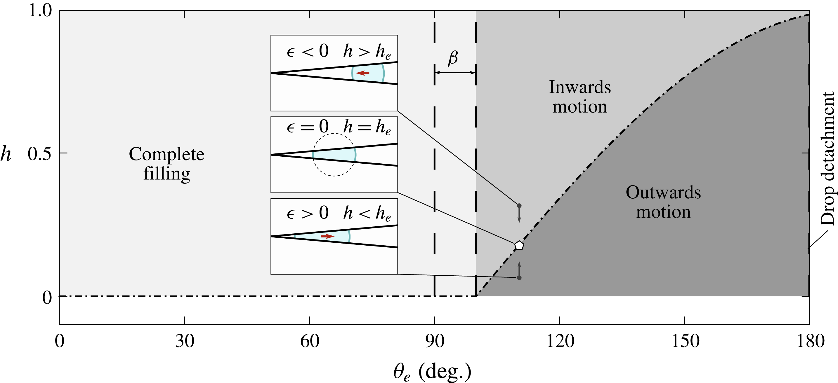
, plays the role of an order parameter. This idea is illustrated in figure 10, which shows a phase diagram of the different filling regimes for a wedge. For
 $\unicode[STIX]{x1D703}\leqslant 90^{\circ }+\unicode[STIX]{x1D6FD}$
,
 $h_{e}=0$
, corresponding to the complete filling states studied by Concus & Finn (Reference Concus and Finn1998), Concus et al. (Reference Concus, Finn and McCuan2001) and Brinkmann & Blossey (Reference Brinkmann and Blossey2004). For
 $\unicode[STIX]{x1D703}_{e}>90^{\circ }+\unicode[STIX]{x1D6FD}$
, corresponding to the barrel regime, the aspect ratio becomes finite, i.e.
 $h_{e}=-\cos (\unicode[STIX]{x1D703}_{e}-\unicode[STIX]{x1D6FD})$
. Increasing the equilibrium contact angle leads to a limiting barrel configuration, where
 $\unicode[STIX]{x1D703}_{e}=180^{\circ }$
and
 $h_{e}=\cos \unicode[STIX]{x1D6FD}$
. In such a limit, the contact area between the liquid and the solid vanishes, and the liquid forms a suspended droplet.
Phase diagram of the filling states of liquid droplets in a solid wedge. The vertical arrows indicate trajectories of the system for fixed values of
 $\unicode[STIX]{x1D703}_{e}$
and
 $\unicode[STIX]{x1D6FD}$
. The dashed line shows the onset of edge blobs. The equilibrium of the trajectories is highlighted and examples of the morphology of the droplet are shown as insets. For clarity, the volume in the examples is not the same.

Out of equilibrium, the instantaneous aspect ratio characterises the inwards and outwards modes of motion for a liquid barrel. Using (2.10) and (2.19) gives
 $$\begin{eqnarray}h=h_{e}\frac{\cos \unicode[STIX]{x1D703}_{e}+(1+\unicode[STIX]{x1D716})\sin \unicode[STIX]{x1D6FD}}{(1+\unicode[STIX]{x1D716})(\cos \unicode[STIX]{x1D703}_{e}+\sin \unicode[STIX]{x1D6FD})}.\end{eqnarray}$$
A displacement of the liquid towards the apex of the wedge will result in a vertical compression of the barrel (see lower inset in figure 10). This corresponds to setting
 $\unicode[STIX]{x1D716}>0$
in (5.1), which leads to a decrease in the aspect ratio, i.e.
 $h<h_{e}$
. In contrast, a displacement towards the wide end of the wedge causes a vertical extension of the interface, and corresponds to
 $\unicode[STIX]{x1D716}<0$
, or, equivalently,
 $h>h_{e}$
. The energy landscapes reported in § 2.4 suggest that the spherical barrel shapes correspond to global minima in the surface energy, and therefore distortions to such shapes will always relax back to equilibrium. For situations where
 $\unicode[STIX]{x1D703}_{e}$
and
 $\unicode[STIX]{x1D6FD}$
are kept constant, trajectories towards equilibrium run as vertical lines in figure 10, pointing towards the master curve
 $h_{e}(\unicode[STIX]{x1D703}_{e}-\unicode[STIX]{x1D6FD})$
.
Baratian et al. (Reference Baratian, Cavalli, van den Ende and Mugele2015) showed that the equilibrium barrel shapes are subject to a vanishing net force. In such a case, the pressure force exerted by the walls on the droplet is exactly balanced by the surface tension acting along the contact line. Out of equilibrium, the net force will not vanish. Because the mean curvature of the barrels is positive, the average Laplace pressure within the droplet is larger than the pressure of the surrounding medium. Therefore, the lateral projection of the pressure force exerted by the liquid on the walls of the wedge points towards the apex, and, consequently, the walls will always exert a reaction force pointing in the outwards direction. On the other hand, the tension acting over the contact line can always be locally decomposed into components that are normal and tangential to the solid surface. In situations where the contact angle is uniform, the integral of the tangential component of the tension force over the contact line will vanish. The vertical component will always point towards the solid, and therefore, the walls will exert a net force pointing inwards. Because a displacement of the barrel towards the narrow end of the wedge always results in an outwards motion, one can infer that the pressure force must be larger than the tension force. On the other hand, the inwards motion of the barrels from the wide end of the wedge towards their equilibrium position suggests that the dynamics is dominated by the tension acting at the contact line. These features are analogous to the well-known problem of capillary invasion (de Gennes, Brochard-Wyart & Quéré Reference de Gennes, Brochard-Wyart and Quéré2004). For tension-dominated dynamics one expects little deviation of the local contact angle from the equilibrium contact angle, similarly to the spontaneous imbibition problem, whilst in the pressure-dominated regime the interface should deform more appreciably from its equilibrium configuration, as in forced imbibition.
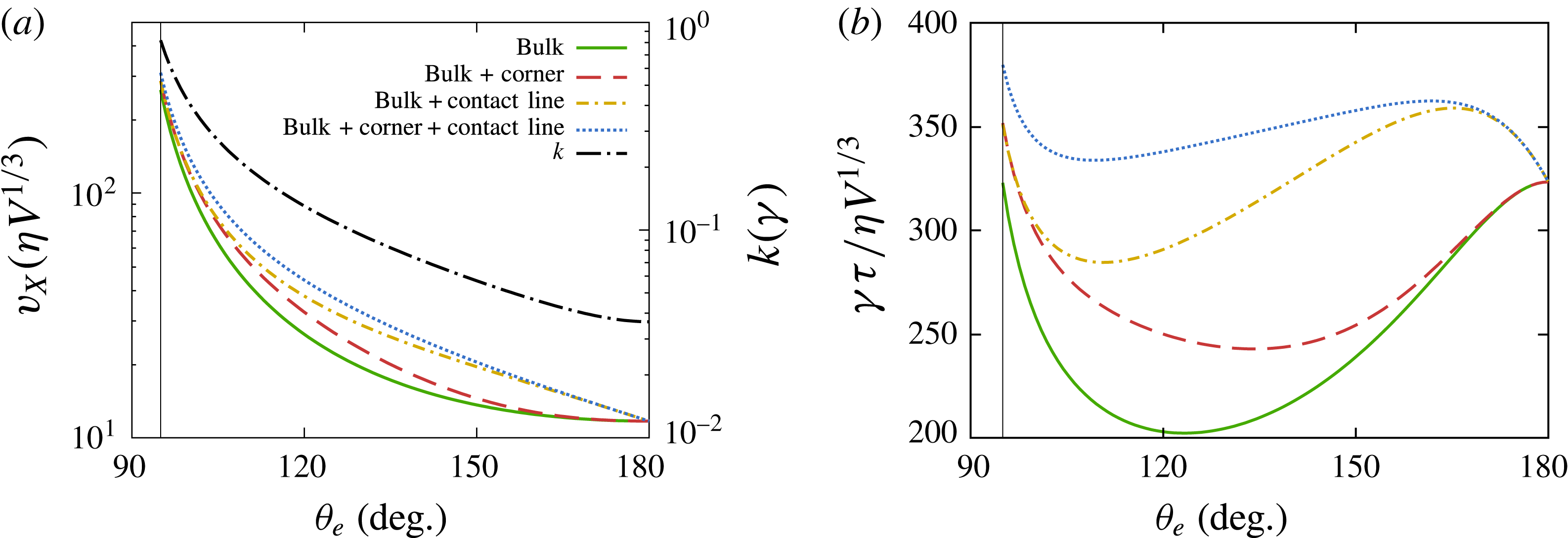
Bulk, corner-flow and contact-line contributions to (a) the drag coefficient,
 $\unicode[STIX]{x1D708}_{X}$
and (b) the relaxation time,
 $\unicode[STIX]{x1D70F}$
, of the translational motion of barrels along the bisector plane of a wedge of angle
 $\unicode[STIX]{x1D6FD}=5^{\circ }$
. In (a) the restitution coefficient,
 $k$
, is superimposed on the right-hand side axis. The vertical lines in both plots correspond to the limiting wetting angle
 $\unicode[STIX]{x1D703}_{e}=90^{\circ }+\unicode[STIX]{x1D6FD}$
.

We close our discussion by focusing on the relaxation time scale of the translational motion of the barrels,
 $\unicode[STIX]{x1D70F}=\unicode[STIX]{x1D708}_{X}/k$
, which results from the balance of the driving capillary force, characterised by the restitution constant
 $k$
, and the overall friction, characterised by the drag coefficient,
 $\unicode[STIX]{x1D708}_{X}$
. Figure 11(a,b) show plots of
 $k$
,
 $\unicode[STIX]{x1D708}_{X}$
and
 $\unicode[STIX]{x1D70F}$
as functions of the equilibrium angle. In the limit
 $\unicode[STIX]{x1D703}_{e}\rightarrow 90^{\circ }+\unicode[STIX]{x1D6FD}$
, the barrel equilibrium position is closer to the apex of the wedge. Geometrically, this implies a stronger confinement, and thus both the bulk contribution to the friction coefficient and the restitution constant reach local maxima in this limit. For larger
 $\unicode[STIX]{x1D703}_{e}$
, both quantities decrease monotonically, leading to an initial decrease in the relaxation time. However, the rate at which
 $k$
decreases becomes dominant with increasing
 $\unicode[STIX]{x1D703}_{e}$
. This is because at higher equilibrium contact angle the barrels keep an approximately spherical shape for larger displacements from equilibrium. As a result, the relaxation time reaches a minimum, beyond which it increases with
 $\unicode[STIX]{x1D703}_{e}$
until it reaches a maximum saturation value as
 $\unicode[STIX]{x1D703}_{e}\rightarrow 180^{\circ }$
. Interestingly, the location of the minimum and maximum relaxation times shown in figure 11(b) depends on the contributions to dissipation from the motion of the corner flow and the contact line.
The typical magnitude of the corner flow is controlled by the length scale separation between the macroscopic length scale,
 $\ell _{M}$
, and the microscopic length scale,
 $\ell _{m}$
. The microscopic length depends on the details of the liquid–gas interactions and the roughness of the solid surface (Bocquet & Charlaix Reference Bocquet and Charlaix2010) that characterise the motion of the interface at the level of the contact line (Snoeijer & Andreotti Reference Snoeijer and Andreotti2013). For a macroscopic droplet, we fix
 $\ell _{M}\sim R_{e}\sim 1~\text{mm}$
and
 $\ell _{m}\sim 10~\text{nm}$
, and thus
 $\ell _{M}/\ell _{m}\approx 10^{5}$
. As shown in figure 11(a), this additional contribution is important at intermediate angles, and vanishes in the limit
 $\unicode[STIX]{x1D703}_{e}\rightarrow 180^{\circ }$
. This is the combined effect of a vanishing contour length and a less confined corner flow at higher opening angle. As a result of the corner flow, the minimum in the relaxation time is displaced to a higher contact angle, as shown in figure 11(b).
The contribution of contact-line dissipation to the drag coefficient is controlled by the (constant) microscopic friction coefficient
 $\unicode[STIX]{x1D701}_{0}$
and the contour length of the contact line. Therefore, this term decays more slowly than the corner-flow term in (4.37). Estimating
 $\unicode[STIX]{x1D701}_{0}$
will, in general, be subject to the details of a specific model (see, e.g. Ranabothu, Karnezis & Dai Reference Ranabothu, Karnezis and Dai2005; S̆ikalo, Tropea & Ganić Reference S̆ikalo, Tropea and Ganić2005). Rather, here we examine the case where
 $\unicode[STIX]{x1D701}_{0}/3\unicode[STIX]{x1D702}=1$
in (4.37) as a specific example where the corner and contact-line dissipation are comparable in magnitude. As shown in figure 11(a,b), the main effect of this term is a slower decay in the contact-line dissipation with increasing contact angle, which in turn leads to an overall broadening of the maximum in the relaxation time.
Experiments of the dynamics of liquid barrels in smooth dry wedge geometries (where a contact line is present) have not yet been reported. Recently, Ruiz-Gutiérrez et al. (Reference Ruiz-Gutiérrez, Guan, Xu, Mchale, Wells and Ledesma-Aguilar2017) have reported experiments of water droplets of volumes in the range of
 $2~\unicode[STIX]{x03BC}\text{l}{-}5~\unicode[STIX]{x03BC}\text{l}$
relaxing towards equilibrium in wedges of opening angles in the range
 $\unicode[STIX]{x1D6FD}=1^{\circ }{-}5^{\circ }$
, where the walls of the wedge are coated with a thin layer of a lubricant oil. The main effect of the lubricant layer is to remove the contact line, whilst introducing a wetting ridge of the lubricant liquid. We thus expect that this system provides a means of testing the bulk contribution to dissipation in our model. Dropping the corner-flow and contact-line contributions to
 $\unicode[STIX]{x1D708}_{X}$
in (4.37), equivalent to setting
 $\unicode[STIX]{x1D701}_{0}=0$
and
 $\ell _{M}/\ell _{m}\approx 1$
, leads to the scaling of the relaxation time
 $$\begin{eqnarray}\unicode[STIX]{x1D70F}\propto \frac{V^{1/3}}{\unicode[STIX]{x1D6FD}^{2}}T(\unicode[STIX]{x1D703}_{e}),\end{eqnarray}$$
where
 $$\begin{eqnarray}T(\unicode[STIX]{x1D703}_{e})=\frac{\cos \unicode[STIX]{x1D703}_{e}}{(\cos 3\unicode[STIX]{x1D703}_{e}-9\cos \unicode[STIX]{x1D703}_{e})^{4/3}}\left[1+\frac{2\cos ^{2}\unicode[STIX]{x1D703}_{e}(\cos 2\unicode[STIX]{x1D703}_{e}-5)}{(2\unicode[STIX]{x1D703}_{e}-\unicode[STIX]{x03C0}-\sin 2\unicode[STIX]{x1D703}_{e})^{2}}\right]^{-1}.\end{eqnarray}$$
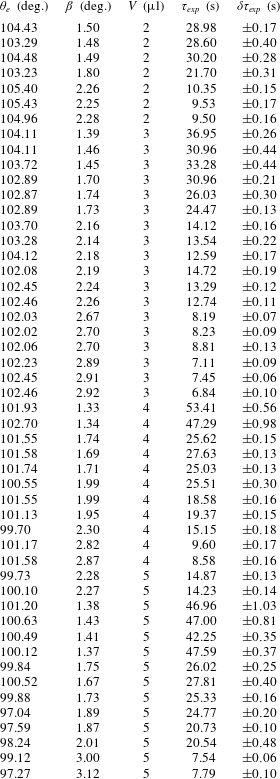
In the experiments of Ruiz-Gutiérrez et al. (Reference Ruiz-Gutiérrez, Guan, Xu, Mchale, Wells and Ledesma-Aguilar2017), the apparent contact angle varies in the range
 $97^{\circ }{-}105^{\circ }$
, with typical experimental errors of
 $1^{\circ }{-}4^{\circ }$
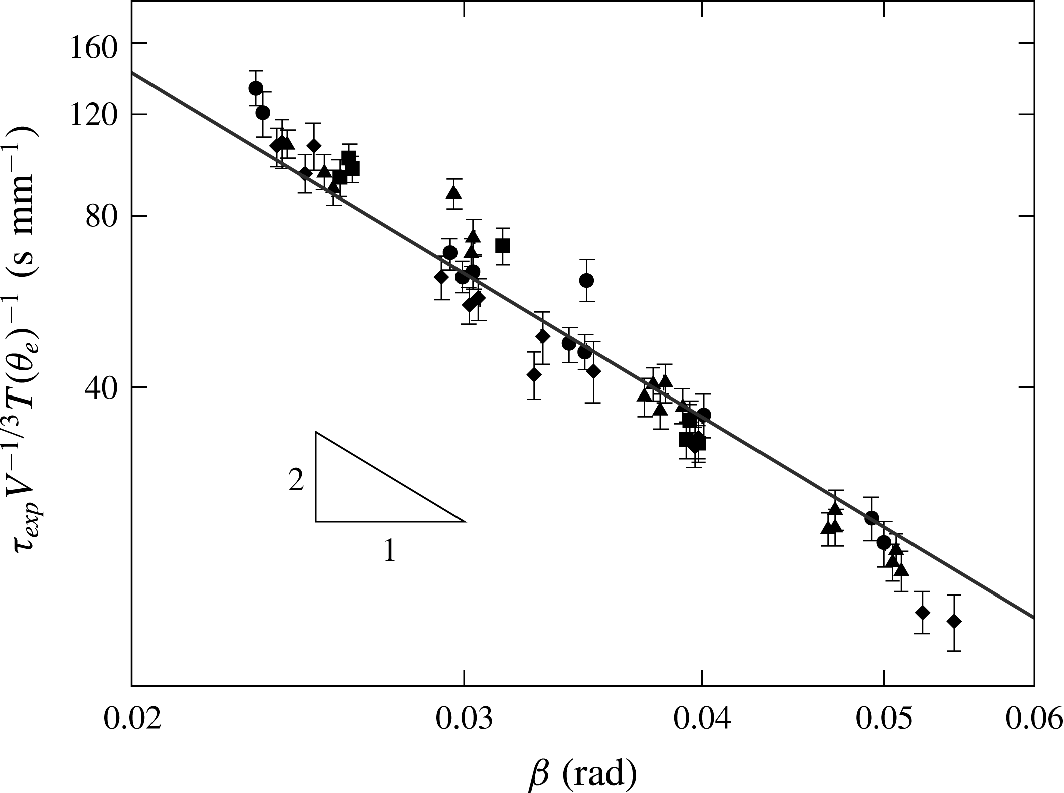
due to the effect of the lubricant layer (see appendix G for a reproduction of the experimental data). Therefore, it is difficult to test the scaling of the relaxation time with the contact angle. In figure 12 we plot the measured relaxation time of Ruiz-Gutiérrez et al. (Reference Ruiz-Gutiérrez, Guan, Xu, Mchale, Wells and Ledesma-Aguilar2017),
 $\unicode[STIX]{x1D70F}_{exp}$
, rescaled by
 $V^{-1/3}T(\unicode[STIX]{x1D703}_{e})^{-1}$
. We obtain a collapse of the experimental data onto a single master curve, which is consistent with the
 ${\sim}\unicode[STIX]{x1D6FD}^{-2}$
scaling predicted by (5.2) over the range of parameters considered. The details of the motion of the droplet in contact with the lubricating layer in the experiments will affect the prefactor in the relaxation time, which our model does not capture, but not the scaling proposed by our theory.
Dependence of the relaxation time data from Ruiz-Gutiérrez et al. (Reference Ruiz-Gutiérrez, Guan, Xu, Mchale, Wells and Ledesma-Aguilar2017), scaled by
 $V^{-1/3}T(\unicode[STIX]{x1D703}_{e})^{-1}$
. The symbols represent different liquid barrel volumes:
 $V=2~\unicode[STIX]{x03BC}\text{l}$
(▪),
 $V=3~\unicode[STIX]{x03BC}\text{l}$
(▴),
 $V=4~\unicode[STIX]{x03BC}\text{l}$
(●), and
 $V=5~\unicode[STIX]{x03BC}\text{l}$
(♦). The solid line represents the theoretical prediction, equation (5.2), up to a best fit of the
 $y$
-intercept to the experimental data.

Therefore, the prediction of the relaxation time can be used in experiments that study the motion of barrels in a wedge geometry to identify the relative contribution of each source of dissipation in the motion of the liquid barrels. More quantitatively, our model can be used to estimate the values of the microscopic cutoff length,
 $\ell _{m}$
, and the friction coefficient,
 $\unicode[STIX]{x1D701}_{0}$
, by treating these quantities as fitting parameters.
Acknowledgements
We would like to thank J. H. Guan and G. G. Wells for bringing to our attention their interesting experimental observations and discussions which partly motivated this work and for kindly sharing their experimental data. We thank F. Mugele for enlightening discussions. É.R.-G. is supported by a Northumbria University PhD Studentship. C.S. acknowledges support from Northumbria University through the Vice-Chancellor’s Fellowship Programme.
Appendix A. Coefficients of the volume and free-energy polynomial forms
Integrating (2.7) with respect to
 $\unicode[STIX]{x1D717}$
gives the following expression for the volume of the liquid,
 $$\begin{eqnarray}\displaystyle V & = & \displaystyle \frac{1}{3}\int _{0}^{2\unicode[STIX]{x03C0}}R\{\!2(X\unicode[STIX]{x2202}_{\unicode[STIX]{x1D711}}r\sin \unicode[STIX]{x1D711}+r^{2}+Xr\cos \unicode[STIX]{x1D711})\sin \unicode[STIX]{x1D713}+R[\!r(3\unicode[STIX]{x1D713}+\sin \unicode[STIX]{x1D713}\cos \unicode[STIX]{x1D713})\nonumber\\ \displaystyle & & \displaystyle +\,X(\unicode[STIX]{x1D713}+\sin \unicode[STIX]{x1D713}\cos \unicode[STIX]{x1D713})\cos \unicode[STIX]{x1D711}\!]+2X\unicode[STIX]{x2202}_{\unicode[STIX]{x1D711}}R\unicode[STIX]{x1D713}\sin \unicode[STIX]{x1D711}+2R^{2}\sin \unicode[STIX]{x1D713}\!\}\,\text{d}\unicode[STIX]{x1D711}.\end{eqnarray}$$
Following the approximations detailed in § 2.2, the radii
 $r$
and
 $R$
read
 $$\begin{eqnarray}\displaystyle & \displaystyle r(\unicode[STIX]{x1D711})=\frac{q\unicode[STIX]{x1D716}\unicode[STIX]{x1D6FC}}{\cos \unicode[STIX]{x1D711}+\unicode[STIX]{x1D6FC}}, & \displaystyle\end{eqnarray}$$
 $$\begin{eqnarray}\displaystyle & \displaystyle R(\unicode[STIX]{x1D711})=q\left(1+\frac{\unicode[STIX]{x1D716}\cos \unicode[STIX]{x1D711}}{\cos \unicode[STIX]{x1D711}+\unicode[STIX]{x1D6FC}}\right), & \displaystyle\end{eqnarray}$$
where
 $\unicode[STIX]{x1D6FC}=-\cos \unicode[STIX]{x1D703}_{e}/\sin \unicode[STIX]{x1D6FD}$
.
Substituting (A 2) and (A 3) into (A 1) results in a polynomial of
 $\unicode[STIX]{x1D716}$
where the coefficients are
 $$\begin{eqnarray}a_{0}=\frac{1}{3}\int _{0}^{2\unicode[STIX]{x03C0}}\{2\sin \unicode[STIX]{x1D713}+\unicode[STIX]{x1D6FC}[\unicode[STIX]{x1D713}+\sin \unicode[STIX]{x1D713}\cos \unicode[STIX]{x1D713}]\cos \unicode[STIX]{x1D711}\}\,\text{d}\unicode[STIX]{x1D711},\end{eqnarray}$$
 $$\begin{eqnarray}\displaystyle a_{1} & = & \displaystyle \frac{1}{6}\int _{0}^{2\unicode[STIX]{x03C0}}(\cos \unicode[STIX]{x1D711}+\unicode[STIX]{x1D6FC})^{-3}\{\!4\unicode[STIX]{x1D6FC}^{4}\cos \unicode[STIX]{x1D711}\sin \unicode[STIX]{x1D713}\nonumber\\ \displaystyle & & \displaystyle +\,\unicode[STIX]{x1D6FC}^{3}[(4\unicode[STIX]{x1D713}+2\sin \unicode[STIX]{x1D713}+\sin 2\unicode[STIX]{x1D713})\cos 2\unicode[STIX]{x1D711}+6(\unicode[STIX]{x1D713}+\sin \unicode[STIX]{x1D713})+2\sin 2\unicode[STIX]{x1D713}]\nonumber\\ \displaystyle & & \displaystyle +\,2\unicode[STIX]{x1D6FC}^{2}[(\{3\unicode[STIX]{x1D713}+\sin 2\unicode[STIX]{x1D713}\}\cos 2\unicode[STIX]{x1D711}+7\unicode[STIX]{x1D713}+4\{2+\cos \unicode[STIX]{x1D713}\}\sin \unicode[STIX]{x1D713})\cos \unicode[STIX]{x1D711}]\nonumber\\ \displaystyle & & \displaystyle +\,\unicode[STIX]{x1D6FC}[(2\unicode[STIX]{x1D713}+\sin 2\unicode[STIX]{x1D713})\cos 2\unicode[STIX]{x1D711}+8\unicode[STIX]{x1D713}+4(6+\cos \unicode[STIX]{x1D713})\sin \unicode[STIX]{x1D713}]\cos ^{2}\unicode[STIX]{x1D711}\nonumber\\ \displaystyle & & \displaystyle +\,12\cos ^{3}\unicode[STIX]{x1D711}\sin \unicode[STIX]{x1D713}\!\}\,\text{d}\unicode[STIX]{x1D711},\end{eqnarray}$$
 $$\begin{eqnarray}\displaystyle a_{2} & = & \displaystyle \frac{1}{12}\int _{0}^{2\unicode[STIX]{x03C0}}(\cos \unicode[STIX]{x1D711}+\unicode[STIX]{x1D6FC})^{-3}\{\!4\unicode[STIX]{x1D6FC}^{3}[\cos 2\unicode[STIX]{x1D711}+3]\sin \unicode[STIX]{x1D713}\nonumber\\ \displaystyle & & \displaystyle +\,\unicode[STIX]{x1D6FC}^{2}[(6\unicode[STIX]{x1D713}+\sin 2\unicode[STIX]{x1D713})\cos 2\unicode[STIX]{x1D711}+22\unicode[STIX]{x1D713}+16\sin \unicode[STIX]{x1D713}+5\sin 2\unicode[STIX]{x1D713}]\cos \unicode[STIX]{x1D711}\nonumber\\ \displaystyle & & \displaystyle +\,\unicode[STIX]{x1D6FC}[(2\unicode[STIX]{x1D713}+\sin 2\unicode[STIX]{x1D713})\cos 2\unicode[STIX]{x1D711}+26\unicode[STIX]{x1D713}+24\sin \unicode[STIX]{x1D713}+5\sin 2\unicode[STIX]{x1D713}]\cos ^{2}\unicode[STIX]{x1D711}\nonumber\\ \displaystyle & & \displaystyle +\,24\cos ^{3}\unicode[STIX]{x1D711}\sin \unicode[STIX]{x1D713}\!\}\,\text{d}\unicode[STIX]{x1D711}\end{eqnarray}$$
and
 $$\begin{eqnarray}a_{3}=\frac{1}{6}\int _{0}^{2\unicode[STIX]{x03C0}}(\cos \unicode[STIX]{x1D711}+\unicode[STIX]{x1D6FC})^{-3}\{4\unicode[STIX]{x1D6FC}^{2}\cos \unicode[STIX]{x1D711}\sin \unicode[STIX]{x1D713}+\unicode[STIX]{x1D6FC}\left[6\unicode[STIX]{x1D713}+\sin 2\unicode[STIX]{x1D713}\right]\cos ^{2}\unicode[STIX]{x1D711}+4\cos ^{3}\unicode[STIX]{x1D711}\sin \unicode[STIX]{x1D713}\}\,\text{d}\unicode[STIX]{x1D711}.\end{eqnarray}$$
The evaluation of the integrals requires an explicit expression of the angle
 $\unicode[STIX]{x1D713}$
; using (2.18) gives
 $$\begin{eqnarray}\tan \unicode[STIX]{x1D713}=\frac{\tan \unicode[STIX]{x1D6FD}}{\unicode[STIX]{x1D6FC}^{2}\tan ^{2}\unicode[STIX]{x1D6FD}-1}\left[\unicode[STIX]{x1D6FC}\sqrt{1+(\cos ^{2}\unicode[STIX]{x1D711}-\unicode[STIX]{x1D6FC}^{2})\tan ^{2}\unicode[STIX]{x1D6FD}}+\cos \unicode[STIX]{x1D711}\right].\end{eqnarray}$$
Using (A 8) and expanding in powers of
 $\unicode[STIX]{x1D6FD}$
leads to (2.26).
To compute the interfacial energy we first note that (2.13) is composed of two terms, the first being
 $$\begin{eqnarray}\int _{0}^{2\unicode[STIX]{x03C0}}\int _{-\unicode[STIX]{x1D713}}^{\unicode[STIX]{x1D713}}|\text{d}\boldsymbol{A}_{lg}|=\int _{0}^{2\unicode[STIX]{x03C0}}\int _{-\unicode[STIX]{x1D713}}^{\unicode[STIX]{x1D713}}R[R^{2}\cos ^{2}\unicode[STIX]{x1D717}+2Rr\cos \unicode[STIX]{x1D717}+r^{2}+(\unicode[STIX]{x2202}_{\unicode[STIX]{x1D711}}R+\unicode[STIX]{x2202}_{\unicode[STIX]{x1D711}}r\cos \unicode[STIX]{x1D717})^{2}]^{1/2}\,\text{d}\unicode[STIX]{x1D717}\,\text{d}\unicode[STIX]{x1D711}.\end{eqnarray}$$
The integral in
 $\unicode[STIX]{x1D717}$
can be expressed in terms of elliptic functions. Then, substituting
 $R$
and
 $r$
using (A 2) and (A 3), gives an expression in terms of
 $q$
and
 $\unicode[STIX]{x1D716}$
. Close to equilibrium
 $\unicode[STIX]{x1D716}\ll 1$
, therefore, we evaluate the integral by first expanding the integrand in powers of
 $\unicode[STIX]{x1D716}$
, which leads to (2.37).
Appendix B. Liquid–gas interface in toroidal coordinates
A position vector in toroidal coordinates has the form,
 $$\begin{eqnarray}\boldsymbol{x}=(x,y,z)=\frac{a}{\unicode[STIX]{x1D6E5}}(\sinh \unicode[STIX]{x1D70E}\cos \unicode[STIX]{x1D714},-\sin \unicode[STIX]{x1D719},\sinh \unicode[STIX]{x1D70E}\sin \unicode[STIX]{x1D714}),\end{eqnarray}$$
where
 $\unicode[STIX]{x1D6E5}=\cosh \unicode[STIX]{x1D70E}-\cos \unicode[STIX]{x1D719}$
, for
 $\unicode[STIX]{x1D70E}\geqslant 0$
,
 $\unicode[STIX]{x1D719}\in (-\unicode[STIX]{x03C0},\unicode[STIX]{x03C0}]$
,
 $\unicode[STIX]{x1D714}\in [-\unicode[STIX]{x1D6FD},\unicode[STIX]{x1D6FD}]$
, and some constant
 $a$
(Andrews Reference Andrews2006; Moon & Spencer Reference Moon and Spencer2012). We have identified the apex of the wedge with the axis of revolution of the angle
 $\unicode[STIX]{x1D714}$
, which are surfaces of constant
 $\unicode[STIX]{x1D70E}$
. The two solid surfaces are planes given by
 $\unicode[STIX]{x1D714}=\pm \unicode[STIX]{x1D6FD}$
, and
 $\unicode[STIX]{x1D714}=0$
corresponds to the bisector plane
 $z=0$
. Higher values of
 $\unicode[STIX]{x1D70E}$
form tori with shrinking tubular radius asymptotically approaching the reference circle,
 $x^{2}+z^{2}=a^{2}$
as
 $\unicode[STIX]{x1D70E}\rightarrow \infty$
. By construction, the shape of the droplet at the bisector plane is a circle with centre at
 $\boldsymbol{X}$
and diameter
 $W$
; using the relation
 $$\begin{eqnarray}(x-a\coth \unicode[STIX]{x1D70E})^{2}+y^{2}=\frac{a^{2}}{\sinh ^{2}\unicode[STIX]{x1D70E}},\end{eqnarray}$$
we can set the value of the constant
 $a$
and the coordinate
 $\unicode[STIX]{x1D70E}$
with the interface of the droplet giving
 $a^{2}=W^{2}(\unicode[STIX]{x1D709}^{2}-1)/4$
, and
 $\cosh \unicode[STIX]{x1D70E}=\unicode[STIX]{x1D709}$
, where
 $\unicode[STIX]{x1D709}=2X/W>1$
. The azimuthal angle of the droplet,
 $\unicode[STIX]{x1D711}$
, and the coordinate
 $\unicode[STIX]{x1D719}$
are related by
 $$\begin{eqnarray}\cos \unicode[STIX]{x1D711}=\frac{\unicode[STIX]{x1D709}\cos \unicode[STIX]{x1D719}-1}{\unicode[STIX]{x1D709}-\cos \unicode[STIX]{x1D719}},\end{eqnarray}$$
at the equatorial circle. Considering that the liquid–gas interface is formed by arcs of constant radii,
 $R$
, and centres at
 $\boldsymbol{X}+\boldsymbol{r}$
, then, equation (2.7) is rewritten as
 $$\begin{eqnarray}[x-(X+r(\unicode[STIX]{x1D711})\cos \unicode[STIX]{x1D711})]^{2}+[y-r(\unicode[STIX]{x1D711})\sin \unicode[STIX]{x1D711}]^{2}+z^{2}=R^{2}(\unicode[STIX]{x1D711});\end{eqnarray}$$
which, by substitution of (B 1) and (B 3), translates into the surface
 $$\begin{eqnarray}\unicode[STIX]{x1D70E}_{lg}(\unicode[STIX]{x1D714})=\log \left[\frac{\unicode[STIX]{x1D6FC}-\unicode[STIX]{x1D709}-(\unicode[STIX]{x1D709}^{2}-1)^{1/2}(1-\unicode[STIX]{x1D6FC}^{2}\sin ^{2}\unicode[STIX]{x1D714})^{1/2}}{\unicode[STIX]{x1D6FC}\unicode[STIX]{x1D709}-1-\unicode[STIX]{x1D6FC}(\unicode[STIX]{x1D709}^{2}-1)^{1/2}\cos \unicode[STIX]{x1D714}}\right],\end{eqnarray}$$
where
 $\unicode[STIX]{x1D6FC}=-\cos \unicode[STIX]{x1D703}_{e}/\sin \unicode[STIX]{x1D6FD}$
.
The normal vector to the surface can be calculated from the gradient of the surface (B 5),
 $$\begin{eqnarray}\hat{\boldsymbol{n}}_{lg}=\frac{\unicode[STIX]{x1D735}(\unicode[STIX]{x1D70E}-\unicode[STIX]{x1D70E}_{lg}(\unicode[STIX]{x1D714}))}{|\unicode[STIX]{x1D735}(\unicode[STIX]{x1D70E}-\unicode[STIX]{x1D70E}_{lg}(\unicode[STIX]{x1D714}))|}=\frac{\sinh \unicode[STIX]{x1D70E}_{lg}\,\hat{\boldsymbol{e}}_{\unicode[STIX]{x1D70E}}-(\unicode[STIX]{x2202}_{\unicode[STIX]{x1D714}}\unicode[STIX]{x1D70E}_{lg})\,\hat{\boldsymbol{e}}_{\unicode[STIX]{x1D714}}}{\sqrt{\sinh ^{2}\unicode[STIX]{x1D70E}_{lg}+(\unicode[STIX]{x2202}_{\unicode[STIX]{x1D714}}\unicode[STIX]{x1D70E}_{lg})^{2}}},\end{eqnarray}$$
where
 $\hat{\boldsymbol{e}}_{i}\equiv \unicode[STIX]{x2202}_{i}\boldsymbol{x}/|\unicode[STIX]{x2202}_{i}\boldsymbol{x}|$
,
 $i=\{\unicode[STIX]{x1D70E},\unicode[STIX]{x1D719},\unicode[STIX]{x1D714}\}$
, are the set of orthonormal coordinate vectors. The normal vector of the interface is useful in the calculation of the mean curvature,
 $2\unicode[STIX]{x1D705}=-\unicode[STIX]{x1D735}\boldsymbol{\cdot }\hat{\boldsymbol{n}}_{lg}$
, which results in
 $$\begin{eqnarray}\unicode[STIX]{x1D705}=\frac{4(\sinh ^{2}\unicode[STIX]{x1D70E}_{lg}-\unicode[STIX]{x0394}\cosh \unicode[STIX]{x1D70E}_{lg})(\unicode[STIX]{x2202}_{\unicode[STIX]{x1D714}}\unicode[STIX]{x1D70E}_{lg})^{2}+\sinh \unicode[STIX]{x1D70E}_{lg}(4\sinh ^{3}\unicode[STIX]{x1D70E}_{lg}-\unicode[STIX]{x0394}\sinh 2\unicode[STIX]{x1D70E}_{lg}+2\unicode[STIX]{x0394}\unicode[STIX]{x2202}_{\unicode[STIX]{x1D714}}^{2}\unicode[STIX]{x1D70E}_{lg})}{4W(\unicode[STIX]{x1D709}^{2}-1)^{1/2}[\sinh ^{2}\unicode[STIX]{x1D70E}_{lg}+(\unicode[STIX]{x2202}_{\unicode[STIX]{x1D714}}\unicode[STIX]{x1D70E}_{lg})^{2}]}.\end{eqnarray}$$
The form of the gradient and divergence can be found in Morse & Feshbach (Reference Morse and Feshbach1953) and Moon & Spencer (Reference Moon and Spencer2012). After evaluating (B 5) in (B 7), we obtain
 $$\begin{eqnarray}\unicode[STIX]{x1D705}=\unicode[STIX]{x1D705}(\unicode[STIX]{x1D719},\unicode[STIX]{x1D714}=0)+\frac{\unicode[STIX]{x1D6FC}(\unicode[STIX]{x1D709}-\unicode[STIX]{x1D6FC})}{4W}\unicode[STIX]{x1D714}^{2}+O(\unicode[STIX]{x1D714}^{4}),\end{eqnarray}$$
where
 $\unicode[STIX]{x1D705}(\unicode[STIX]{x1D719},\unicode[STIX]{x1D714}=0)$
is the curvature at the equatorial plane,
 $$\begin{eqnarray}\unicode[STIX]{x1D705}(\unicode[STIX]{x1D719},\unicode[STIX]{x1D714}=0)=\frac{2}{W}\left[1+\frac{(\unicode[STIX]{x1D6FC}-\unicode[STIX]{x1D709})(\unicode[STIX]{x1D709}-\cos \unicode[STIX]{x1D719})}{2(\unicode[STIX]{x1D709}^{2}-1)}\right].\end{eqnarray}$$
Considering that
 $|\unicode[STIX]{x1D714}|\leqslant \unicode[STIX]{x1D6FD}$
and
 $\unicode[STIX]{x1D709}\sim \unicode[STIX]{x1D6FC}$
near equilibrium, the correction term in (B 8) is vanishingly small. Substituting (B 3) into (B 9) gives (2.44).
Appendix C. Pressure profile
In toroidal coordinates, introduced in appendix B, Laplace’s equation for the pressure field (2.41) reads (see, e.g. Moon & Spencer Reference Moon and Spencer2012)
 $$\begin{eqnarray}\unicode[STIX]{x1D6FB}^{2}p=\frac{\unicode[STIX]{x1D6E5}^{3}}{a^{2}\sinh \unicode[STIX]{x1D70E}}\left[\unicode[STIX]{x2202}_{\unicode[STIX]{x1D70E}}\left(\frac{\sinh \unicode[STIX]{x1D70E}}{\unicode[STIX]{x1D6E5}}\unicode[STIX]{x2202}_{\unicode[STIX]{x1D70E}}p\right)+\unicode[STIX]{x2202}_{\unicode[STIX]{x1D719}}\left(\frac{\sinh \unicode[STIX]{x1D70E}}{\unicode[STIX]{x1D6E5}}\unicode[STIX]{x2202}_{\unicode[STIX]{x1D719}}p\right)\right]+\frac{\unicode[STIX]{x1D6E5}^{2}}{a^{2}\sinh ^{2}\unicode[STIX]{x1D70E}}\unicode[STIX]{x2202}_{\unicode[STIX]{x1D714}}^{2}p=0.\end{eqnarray}$$
This equation is separable using the ansatz
 $p=(\unicode[STIX]{x1D6E5}/\sinh \unicode[STIX]{x1D70E})^{1/2}S(\unicode[STIX]{x1D70E})\unicode[STIX]{x1D6F7}(\unicode[STIX]{x1D719})\unicode[STIX]{x1D6FA}(\unicode[STIX]{x1D714})$
. The general solution is given by Andrews (Reference Andrews2006), where
 $S(\unicode[STIX]{x1D70E})$
is expressed as a linear combination of terms
 $P_{\unicode[STIX]{x1D708}-1/2}^{\unicode[STIX]{x1D707}}(\coth \unicode[STIX]{x1D70E})$
and
 $Q_{\unicode[STIX]{x1D708}-1/2}^{\unicode[STIX]{x1D707}}(\coth \unicode[STIX]{x1D70E})$
, which are the Legendre and associate Legendre functions of the third kind;
 $\unicode[STIX]{x1D6F7}(\unicode[STIX]{x1D719})$
is expressed as a linear combination of the functions
 $\cos m\unicode[STIX]{x1D719}$
and
 $\sin m\unicode[STIX]{x1D719}$
; and
 $\unicode[STIX]{x1D6FA}(\unicode[STIX]{x1D714})$
as a linear combination of terms
 $\cos \unicode[STIX]{x1D707}\unicode[STIX]{x1D714}$
and
 $\sin \unicode[STIX]{x1D707}\unicode[STIX]{x1D714}$
.
Periodicity in the angle
 $\unicode[STIX]{x1D719}$
demands that
 $p(\unicode[STIX]{x1D719}+2\unicode[STIX]{x03C0})=p(\unicode[STIX]{x1D719})$
for all
 $\unicode[STIX]{x1D719}$
, therefore making
 $m$
an integer, and, due to the plane symmetry (
 $y\leftrightarrow -y$
) we only keep the
 $\cos m\unicode[STIX]{x1D719}$
solutions. Symmetry upon a reflection about the bisector plane (
 $z\leftrightarrow -z$
) allows us to only keep solutions of the form
 $\cos \unicode[STIX]{x1D707}\unicode[STIX]{x1D714}$
. The boundary condition at the solid surface,
 $\unicode[STIX]{x2202}_{\unicode[STIX]{x1D714}}p(\unicode[STIX]{x1D6FD})=0$
, sets
 $\unicode[STIX]{x1D707}=\unicode[STIX]{x03C0}n/\unicode[STIX]{x1D6FD}$
, for integer
 $n$
. Interior solutions, i.e. finite value at the inner phase, demand discarding the
 $Q_{\unicode[STIX]{x1D707}-1/2}^{m}$
terms since they diverge at the reference circle. After these simplifications, the pressure field is expressed as
 $$\begin{eqnarray}p=\frac{4\unicode[STIX]{x1D6FE}}{W}\mathop{\sum }_{m,n=0}^{\infty }A_{mn}\unicode[STIX]{x1D6F9}_{mn}(\unicode[STIX]{x1D70E},\unicode[STIX]{x1D719},\unicode[STIX]{x1D714}),\end{eqnarray}$$
where
 $$\begin{eqnarray}\unicode[STIX]{x1D6F9}_{mn}(\unicode[STIX]{x1D70E},\unicode[STIX]{x1D719},\unicode[STIX]{x1D714})=\left[\frac{\cosh \unicode[STIX]{x1D70E}-\cos \unicode[STIX]{x1D719}}{\sinh \unicode[STIX]{x1D70E}}\right]^{1/2}P_{\unicode[STIX]{x03C0}n/\unicode[STIX]{x1D6FD}-1/2}^{m}(\coth \unicode[STIX]{x1D70E})\cos (m\unicode[STIX]{x1D719})\cos (\unicode[STIX]{x03C0}n\unicode[STIX]{x1D714}/\unicode[STIX]{x1D6FD}).\end{eqnarray}$$
Note that for small
 $\unicode[STIX]{x1D6FD}$
, the lower index in the Legendre function becomes large and so does its value at the boundary. This implies that the terms of higher order in
 $n$
should carry a vanishingly small coefficient; and, even for
 $n=1$
, their contribution can be neglected. Therefore, the pressure at the equatorial circle of the droplet which can be written as
 $(4\unicode[STIX]{x1D6FE}/W)\sum _{k=0}^{1}c_{k}\cos k\unicode[STIX]{x1D719}$
, where the coefficients
 $c_{k}=c_{k}(\unicode[STIX]{x1D709},\unicode[STIX]{x1D6FC})$
are
 $$\begin{eqnarray}\displaystyle & \displaystyle c_{0}=\frac{\unicode[STIX]{x1D709}^{2}+\unicode[STIX]{x1D6FC}\unicode[STIX]{x1D709}-2}{2(\unicode[STIX]{x1D709}^{2}-1)}, & \displaystyle\end{eqnarray}$$
 $$\begin{eqnarray}\displaystyle & \displaystyle c_{1}=\frac{\unicode[STIX]{x1D709}-\unicode[STIX]{x1D6FC}}{2(\unicode[STIX]{x1D709}^{2}-1)}. & \displaystyle\end{eqnarray}$$
As stated in Andrews (Reference Andrews2006, appendix B), the prefactor in square brackets from the general solution, equation (C 3), can be expressed as a Fourier cosine series,
 $$\begin{eqnarray}\frac{1}{\sqrt{\unicode[STIX]{x1D709}-\cos \unicode[STIX]{x1D719}}}=\mathop{\sum }_{m=0}^{\infty }b_{m}(\unicode[STIX]{x1D709})\cos m\unicode[STIX]{x1D719},\end{eqnarray}$$
where
 $b_{m}=(2^{1/2}/\unicode[STIX]{x03C0})(2-\unicode[STIX]{x1D6FF}_{0m})Q_{m-1/2}(\unicode[STIX]{x1D709})$
.
The product of the two Fourier series can be recast into a single series by using the trigonometric equality,
 $2\cos m\unicode[STIX]{x1D719}\cos k\unicode[STIX]{x1D719}=\cos [(m+k)\unicode[STIX]{x1D719}]+\cos [(m-k)\unicode[STIX]{x1D719}]$
, and rearranging terms; then, the
 $A_{m0}$
coefficients are
 $$\begin{eqnarray}A_{m0}(\unicode[STIX]{x1D709},\unicode[STIX]{x1D6FC})=\frac{(\unicode[STIX]{x1D709}^{2}-1)^{1/4}}{P_{-1/2}^{m}(\unicode[STIX]{x1D709}/\sqrt{\unicode[STIX]{x1D709}^{2}-1})}\times \left\{\begin{array}{@{}ll@{}}c_{0}b_{0}+c_{1}b_{1}/2,\quad & m=0,\\ c_{0}b_{1}+c_{1}(b_{0}+b_{2}/2),\quad & m=1,\\ c_{0}b_{m}+c_{1}(b_{m-1}+b_{m+1})/2,\quad & m\geqslant 2.\end{array}\right.\end{eqnarray}$$
Appendix D. Jeffery–Hamel flow
The flow within a wedge geometry, including inertial effects, was addressed by Rosenhead (Reference Rosenhead1940). Here we follow a similar procedure to obtain the low-Reynolds-number behaviour of the flow. Using the polar coordinates
 $s^{2}=x^{2}+z^{2}$
and
 $\unicode[STIX]{x1D714}=\arctan (z/x)$
, the velocity field is expressed as
 $\boldsymbol{u}_{bulk}=u_{s}\hat{\boldsymbol{s}}+u_{\unicode[STIX]{x1D714}}\hat{\unicode[STIX]{x1D74E}}$
where the angular flow is assumed to vanish, i.e.
 $u_{\unicode[STIX]{x1D714}}=0$
.
The continuity equation, (2.40), reads
 $$\begin{eqnarray}\frac{1}{s}\frac{\unicode[STIX]{x2202}su_{s}}{\unicode[STIX]{x2202}s}=0,\end{eqnarray}$$
which has the general solution,
 $$\begin{eqnarray}u_{s}(s,\unicode[STIX]{x1D714})=\frac{f(\unicode[STIX]{x1D714})}{s},\end{eqnarray}$$
where
 $f$
depends only on
 $\unicode[STIX]{x1D714}$
. The explicit form of
 $f$
can be found using the Stokes equations, (2.39). In polar coordinates, and using (D 2), these read
 $$\begin{eqnarray}\displaystyle & \displaystyle \unicode[STIX]{x1D702}\frac{f^{\prime \prime }}{s^{3}}-\frac{\unicode[STIX]{x2202}p_{bulk}}{\unicode[STIX]{x2202}s}=0, & \displaystyle\end{eqnarray}$$
 $$\begin{eqnarray}\displaystyle & \displaystyle 2\unicode[STIX]{x1D702}\frac{f^{\prime }}{s^{3}}-\frac{1}{s}\frac{\unicode[STIX]{x2202}p_{bulk}}{\unicode[STIX]{x2202}\unicode[STIX]{x1D714}}=0. & \displaystyle\end{eqnarray}$$
Integrating (D 4) with respect to
 $\unicode[STIX]{x1D714}$
gives the pressure profile,
 $$\begin{eqnarray}p_{bulk}(s,\unicode[STIX]{x1D714})=\frac{2\unicode[STIX]{x1D702}}{s^{2}}f(\unicode[STIX]{x1D714})+g(s),\end{eqnarray}$$
where
 $g$
only depends on
 $s$
. Substituting this result into (D 3) gives the equation,
 $$\begin{eqnarray}\frac{\text{d}^{2}f}{\text{d}\unicode[STIX]{x1D714}^{2}}+4f=\frac{s^{3}}{\unicode[STIX]{x1D702}}\frac{\text{d}g}{\text{d}s}.\end{eqnarray}$$
The left-hand side only depends on
 $\unicode[STIX]{x1D714}$
, whereas the right-hand side only depends on
 $s$
. This can only happen if both sides are equal to a constant,
 $c_{1}$
. Therefore,
 $$\begin{eqnarray}g(s)=-\frac{c_{1}\unicode[STIX]{x1D702}}{2s^{2}}+c_{2},\quad \text{and}\quad f(\unicode[STIX]{x1D714})=\frac{c_{1}}{4}+c_{3}\cos 2\unicode[STIX]{x1D714}+c_{4}\sin 2\unicode[STIX]{x1D714}.\end{eqnarray}$$
The constants
 $c_{i}$
,
 $i=1,\ldots ,4$
can be found by imposing boundary conditions to the flow. Due to symmetry, the flow profile must be an even function of
 $\unicode[STIX]{x1D714}$
, therefore
 $c_{4}=0$
. Imposing a no-slip boundary condition at the walls of the wedge fixes
 $c_{1}=-4c_{3}\cos 2\unicode[STIX]{x1D6FD}$
. Setting the pressure to
 $p_{bulk}(s_{1})=p_{1}$
and
 $p_{bulk}(s_{2})=p_{2}$
at two arbitrary points,
 $s_{1}$
and
 $s_{2}$
, fixes
 $c_{2}=(p_{1}s_{1}^{2}-p_{2}s_{2}^{2})/(s_{1}^{2}-s_{2}^{2})$
and
 $c_{3}=(p_{2}-p_{1})s_{1}^{2}s_{2}^{2}/2\unicode[STIX]{x1D702}(s_{1}^{2}-s_{2}^{2})$
.
To express the flow field in terms of the velocity of the droplet, we match the average of
 $\boldsymbol{u}_{bulk}$
to
 ${\dot{X}}$
, i.e.
 $$\begin{eqnarray}\displaystyle {\dot{X}} & = & \displaystyle \left[\int _{-\unicode[STIX]{x1D6FD}}^{\unicode[STIX]{x1D6FD}}\int _{s_{1}}^{s_{2}}s\,\text{d}s\,\text{d}\unicode[STIX]{x1D714}\right]^{-1}\int _{-\unicode[STIX]{x1D6FD}}^{\unicode[STIX]{x1D6FD}}\int _{s_{1}}^{s_{2}}\boldsymbol{u}_{bulk}\boldsymbol{\cdot }\hat{\boldsymbol{s}}s\,\text{d}s\,\text{d}\unicode[STIX]{x1D714}\end{eqnarray}$$
 $$\begin{eqnarray}\displaystyle & = & \displaystyle -\frac{p_{1}-p_{2}}{s_{1}-s_{2}}\left(\frac{s_{1}s_{2}}{s_{1}+s_{2}}\right)^{2}\frac{\sin 2\unicode[STIX]{x1D6FD}-2\unicode[STIX]{x1D6FD}\cos 2\unicode[STIX]{x1D6FD}}{2\unicode[STIX]{x1D6FD}\unicode[STIX]{x1D702}}.\end{eqnarray}$$
Therefore, the bulk velocity field reads
 $$\begin{eqnarray}\boldsymbol{u}_{bulk}={\dot{X}}\frac{s_{1}+s_{2}}{2s}\frac{\cos 2\unicode[STIX]{x1D6FD}-\cos 2\unicode[STIX]{x1D714}}{\cos 2\unicode[STIX]{x1D6FD}-\unicode[STIX]{x1D6FD}^{-1}\sin 2\unicode[STIX]{x1D6FD}}\hat{\boldsymbol{s}}.\end{eqnarray}$$
Converting this expression to Cartesian coordinates and making the substitutions
 $s_{1}=X-W/2$
and
 $s_{2}=X+W/2$
leads to (4.16). To obtain the pressure profiles in figure 9 we use
 $p_{1}=2\unicode[STIX]{x1D6FE}\unicode[STIX]{x1D705}(\unicode[STIX]{x03C0},0)$
and
 $p_{2}=2\unicode[STIX]{x1D6FE}\unicode[STIX]{x1D705}(0,0)$
to fix the constants in (D 5), where
 $\unicode[STIX]{x1D705}$
is given by (2.44).
Appendix E. Bulk dissipation
By substituting (D 10) in (4.24), we can determine the energy dissipation in the bulk of the droplet. First, the gradient of the velocity field is
 $$\begin{eqnarray}\unicode[STIX]{x1D735}\boldsymbol{u}_{bulk}=\frac{{\dot{X}}\unicode[STIX]{x1D6FD}(s_{1}+s_{2})}{s^{2}(2\unicode[STIX]{x1D6FD}\cos 2\unicode[STIX]{x1D6FD}-\sin 2\unicode[STIX]{x1D6FD})}\left[\begin{array}{@{}cc@{}}\cos 2\unicode[STIX]{x1D714}-\cos 2\unicode[STIX]{x1D6FD} & \sin 2\unicode[STIX]{x1D714}\\ 0 & \cos 2\unicode[STIX]{x1D6FD}-\cos 2\unicode[STIX]{x1D714}\end{array}\right],\end{eqnarray}$$
which leads to the bulk energy dissipation density
 $$\begin{eqnarray}\dot{\unicode[STIX]{x1D700}}=-\frac{\unicode[STIX]{x1D702}}{2}(\unicode[STIX]{x1D735}\boldsymbol{u}_{bulk}+\unicode[STIX]{x1D735}\boldsymbol{u}_{bulk}^{\text{T}})^{2}=\frac{2\unicode[STIX]{x1D702}{\dot{X}}^{2}\unicode[STIX]{x1D6FD}^{2}(s_{1}+s_{2})^{2}(3+\cos 4\unicode[STIX]{x1D6FD}-4\cos 2\unicode[STIX]{x1D6FD}\cos 2\unicode[STIX]{x1D714})}{s^{4}(2\unicode[STIX]{x1D6FD}\cos 2\unicode[STIX]{x1D6FD}-\sin 2\unicode[STIX]{x1D6FD})^{2}}.\end{eqnarray}$$
To obtain the total dissipation, equation (E 2) needs to be integrated over a volume
 $V_{eff}<V$
, that corresponds to the region where the approximation of a Jeffery–Hamel flow is adequate and thus the bulk dissipation of the barrel takes place.
We approximate
 $V_{eff}$
, as a toroidal section, of major radius equal to the distance
 $X$
, and a minor diameter
 $W^{\prime }=W-\unicode[STIX]{x1D6FF}$
, for some positive
 $\unicode[STIX]{x1D6FF}\ll W$
. Therefore, the bulk dissipation is
 $$\begin{eqnarray}\dot{{\mathcal{E}}}_{bulk}=\int \dot{\unicode[STIX]{x1D700}}\,\text{d}V_{eff}=\int _{-\unicode[STIX]{x1D6FD}}^{\unicode[STIX]{x1D6FD}}\int _{X-W^{\prime }/2}^{X+W^{\prime }/2}\int _{-\sqrt{{W^{\prime }}^{2}/4-(s-X)^{2}}}^{\sqrt{{W^{\prime }}^{2}/4-(s-X)^{2}}}\dot{\unicode[STIX]{x1D700}}\,\text{d}y\,s\,\text{d}s\,\text{d}\unicode[STIX]{x1D714},\end{eqnarray}$$
which evaluates to
 $$\begin{eqnarray}\dot{{\mathcal{E}}}_{bulk}\approx -\frac{32\unicode[STIX]{x03C0}\unicode[STIX]{x1D702}\unicode[STIX]{x1D6FD}^{2}{\dot{X}}^{2}W^{2}X^{2}[\unicode[STIX]{x1D6FD}(\cos 4\unicode[STIX]{x1D6FD}+3)-\sin 4\unicode[STIX]{x1D6FD}]}{(4X^{2}-W^{2})^{3/2}(2\unicode[STIX]{x1D6FD}\cos 2\unicode[STIX]{x1D6FD}-\sin 2\unicode[STIX]{x1D6FD})^{2}}.\end{eqnarray}$$
Taking a Laurent series expansion in
 $\unicode[STIX]{x1D6FD}$
of (E 4) leads to (4.24).
Appendix F. The contour integral of the velocity of the contact line
To calculate the closed-loop integral in (4.28), and (4.30), we first obtain
 $v_{cl}$
, the projection of the velocity perpendicular to the contact line. This can be done by obtaining a parametrisation of the contact line. Points belonging to the contact line can be reached through three displacements from the origin, that is,
 $$\begin{eqnarray}\boldsymbol{x}_{cl}=X\hat{\boldsymbol{x}}+X\sin \unicode[STIX]{x1D6FD}\hat{\boldsymbol{n}}+\boldsymbol{r}_{cl}.\end{eqnarray}$$
The first displacement lands in the centre of the droplet, from there, the next displacement moves to the nearest point in the top solid surface, concluding with a coplanar displacement to the triple line represented by the vector
 $\boldsymbol{r}_{cl}$
. This vector can be obtained using (2.7) evaluated at the boundary. Then,
 $\boldsymbol{r}_{cl}=\boldsymbol{x}_{lg}(\unicode[STIX]{x1D711},\unicode[STIX]{x1D717}=\unicode[STIX]{x1D713})-X\hat{\boldsymbol{x}}-X\sin \unicode[STIX]{x1D6FD}\,\hat{\boldsymbol{n}}$
, which gives the radius of the contact line,
 $$\begin{eqnarray}\displaystyle r_{cl} & = & \displaystyle \frac{q}{2(\unicode[STIX]{x1D6FC}+\cos \unicode[STIX]{x1D711})} [\!2(1+\unicode[STIX]{x1D716})^{2}+\unicode[STIX]{x1D6FC}^{2}(3-2\unicode[STIX]{x1D6FC}^{2}+4\unicode[STIX]{x1D716}^{2})-4\unicode[STIX]{x1D6FC}\{\unicode[STIX]{x1D6FC}^{2}-2(1+\unicode[STIX]{x1D716})\}\cos \unicode[STIX]{x1D711}\nonumber\\ \displaystyle & & \displaystyle +\,2\unicode[STIX]{x1D6FC}\cos 2\unicode[STIX]{x1D6FD}(\unicode[STIX]{x1D6FC}+\cos \unicode[STIX]{x1D711})^{2}+\{2(1+\unicode[STIX]{x1D716})^{2}-\unicode[STIX]{x1D6FC}^{2}\}\cos 2\unicode[STIX]{x1D711}\nonumber\\ \displaystyle & & \displaystyle +\,8\unicode[STIX]{x1D6FC}\unicode[STIX]{x1D716}\{\unicode[STIX]{x1D6FC}+(1+\unicode[STIX]{x1D716})\cos \unicode[STIX]{x1D711}\}\cos \unicode[STIX]{x1D713}]^{1/2},\end{eqnarray}$$
where we have used the relation,
 $\sin \unicode[STIX]{x1D713}=(\unicode[STIX]{x1D6FC}+\cos \unicode[STIX]{x1D711}\cos \unicode[STIX]{x1D713})\tan \unicode[STIX]{x1D6FD}$
, that results from (2.18), to simplify the expression. Substituting (A 8), the contact-line radius can be expressed in series form,
 $$\begin{eqnarray}r_{cl}=q(1+\unicode[STIX]{x1D716})-{\textstyle \frac{1}{2}}q\unicode[STIX]{x1D6FC}\unicode[STIX]{x1D6FD}^{2}(\unicode[STIX]{x1D6FC}+\unicode[STIX]{x1D716}\cos \unicode[STIX]{x1D711})+O(\unicode[STIX]{x1D6FD}^{3}).\end{eqnarray}$$
Notice that at
 $\unicode[STIX]{x1D716}=0$
, the variation in
 $\unicode[STIX]{x1D711}$
from (F 2), is lost and the contact line becomes a circle. From (F 3), we can see the that dependence in
 $\unicode[STIX]{x1D711}$
is weak, since it is proportional to
 $\unicode[STIX]{x1D6FC}\unicode[STIX]{x1D6FD}^{2}\unicode[STIX]{x1D716}\sim \unicode[STIX]{x1D6FD}\unicode[STIX]{x1D716}$
.
After obtaining the magnitude of the vector
 $\boldsymbol{r}_{cl}$
, its direction can be expressed by the unitary vector
 $\hat{\boldsymbol{r}}_{cl}=\boldsymbol{r}_{cl}/r_{cl}$
. From (F 1), (A 8) and (F 2), we can see that
 $$\begin{eqnarray}\hat{\boldsymbol{r}}_{cl}=\frac{(\cos \unicode[STIX]{x1D711},\sin \unicode[STIX]{x1D711},\tan \unicode[STIX]{x1D6FD}\cos \unicode[STIX]{x1D711})}{\sqrt{1+\tan ^{2}\unicode[STIX]{x1D6FD}\cos ^{2}\unicode[STIX]{x1D711}}}+O(\unicode[STIX]{x1D6FD}^{4},\unicode[STIX]{x1D716}).\end{eqnarray}$$
This a vector collinear to the intersection of the solid plane wall, and a vertical slice at the angle
 $\unicode[STIX]{x1D711}$
from the
 $x$
axis.
Experimental measurements of the translational relaxation time,
 $\unicode[STIX]{x1D70F}_{exp}$
, of a droplet in a wedge geometry, reproduced from Ruiz-Gutiérrez et al. (Reference Ruiz-Gutiérrez, Guan, Xu, Mchale, Wells and Ledesma-Aguilar2017).

The velocity of the points in the contact line can be calculated by the derivative with respect to time of (F 1); using (2.27), (F 2) and (F 4), this is
 $$\begin{eqnarray}\displaystyle \boldsymbol{v}_{cl} & = & \displaystyle \left({\textstyle \frac{1}{2}} [\!q\cos \unicode[STIX]{x1D711}\{2-\unicode[STIX]{x1D6FD}^{2}\cos ^{2}\unicode[STIX]{x1D711}\}\dot{\unicode[STIX]{x1D716}}-\dot{q}\{(\unicode[STIX]{x1D6FC}^{2}\unicode[STIX]{x1D6FD}^{2}-2)\cos \unicode[STIX]{x1D711}+2\unicode[STIX]{x1D6FC}(\unicode[STIX]{x1D6FD}^{2}-1)+\unicode[STIX]{x1D6FD}^{2}\cos ^{3}\unicode[STIX]{x1D711}\right.\nonumber\\ \displaystyle & & \displaystyle +\,\unicode[STIX]{x1D716}\cos \unicode[STIX]{x1D711}(\unicode[STIX]{x1D6FD}^{2}\cos ^{2}\unicode[STIX]{x1D711}-2)\!\}\!],\nonumber\\ \displaystyle & & \displaystyle -\,{\textstyle \frac{1}{2}}\sin \unicode[STIX]{x1D711}[\dot{q}\{\unicode[STIX]{x1D6FC}^{2}\unicode[STIX]{x1D6FD}^{2}+\unicode[STIX]{x1D6FD}^{2}\cos ^{2}\unicode[STIX]{x1D711}+\unicode[STIX]{x1D716}(\unicode[STIX]{x1D6FD}^{2}\cos ^{2}\unicode[STIX]{x1D711}-2)-2\}+q(\unicode[STIX]{x1D6FD}^{2}\cos ^{2}\unicode[STIX]{x1D711}-2)\dot{\unicode[STIX]{x1D716}}],\nonumber\\ \displaystyle & & \displaystyle \left.\unicode[STIX]{x1D6FD}[\dot{q}(\unicode[STIX]{x1D6FC}+\unicode[STIX]{x1D716}\cos \unicode[STIX]{x1D711}+\cos \unicode[STIX]{x1D711})+q\cos \unicode[STIX]{x1D711}\dot{\unicode[STIX]{x1D716}}]\vphantom{{\textstyle \frac{1}{2}}}\right)+\boldsymbol{O}(\unicode[STIX]{x1D6FD}^{3}).\end{eqnarray}$$
To calculate the projection of the velocity in the perpendicular direction to the contact line, we define the vector
 $\hat{\boldsymbol{b}}\equiv \hat{\boldsymbol{t}}\times \hat{\boldsymbol{n}}$
, where
 $\hat{\boldsymbol{t}}=\unicode[STIX]{x2202}_{\unicode[STIX]{x1D711}}\boldsymbol{r}_{cl}/|\unicode[STIX]{x2202}_{\unicode[STIX]{x1D711}}\boldsymbol{r}_{cl}|$
. For the sake of simplicity, we shall use,
 $\hat{\boldsymbol{b}}=\hat{\boldsymbol{r}}_{cl}$
, which is a valid approximation for small values of
 $\unicode[STIX]{x1D6FD}$
and
 $\unicode[STIX]{x1D716}$
. Then, the projected velocity reads
 $$\begin{eqnarray}v_{cl}\approx \boldsymbol{v}_{cl}\boldsymbol{\cdot }\hat{\boldsymbol{r}}_{cl}=q\dot{\unicode[STIX]{x1D716}}-\frac{\dot{q}}{4}[2\unicode[STIX]{x1D6FC}^{2}\unicode[STIX]{x1D6FD}^{2}+\unicode[STIX]{x1D6FC}(\unicode[STIX]{x1D6FD}^{2}(1+\cos (2\unicode[STIX]{x1D711}))-4)\cos \unicode[STIX]{x1D711}-4(1+\unicode[STIX]{x1D716})]+O(\unicode[STIX]{x1D6FD}^{3}).\end{eqnarray}$$
We now have all the ingredients to compute the circuit integral. The infinitesimal length
 $\text{d}l$
becomes
 $r_{cl}\text{d}\unicode[STIX]{x1D711}$
, and the integration is performed over the interval
 $[0,\,2\unicode[STIX]{x03C0}]$
. The integral in (4.29) can be evaluated in series form,
 $$\begin{eqnarray}\displaystyle \oint _{cl}v_{cl}^{2}\,\text{d}l\approx \int _{0}^{2\unicode[STIX]{x03C0}}v_{cl}^{2}r_{cl}\,\text{d}\unicode[STIX]{x1D711} & = & \displaystyle \unicode[STIX]{x03C0}q(1+\unicode[STIX]{x1D716})[\{\unicode[STIX]{x1D6FC}^{2}+2(1+\unicode[STIX]{x1D716})^{2}\}\dot{q}^{2}+4q(1+\unicode[STIX]{x1D716})\dot{\unicode[STIX]{x1D716}}\dot{q}+2q^{2}\dot{\unicode[STIX]{x1D716}}^{2}]\nonumber\\ \displaystyle & & \displaystyle -\,\frac{\unicode[STIX]{x03C0}}{4}\unicode[STIX]{x1D6FC}^{2}\unicode[STIX]{x1D6FD}^{2}q[\{2\unicode[STIX]{x1D6FC}^{2}+3(1+\unicode[STIX]{x1D716})(5+4\unicode[STIX]{x1D716})\}\dot{q}^{2}\nonumber\\ \displaystyle & & \displaystyle +\,16q(1+\unicode[STIX]{x1D716})\dot{\unicode[STIX]{x1D716}}\dot{q}+4q^{2}\dot{\unicode[STIX]{x1D716}}^{2}\! ]+O(\unicode[STIX]{x1D6FD}^{4}).\end{eqnarray}$$
Substituting
 $\unicode[STIX]{x1D6FC}=-\cos \unicode[STIX]{x1D703}_{e}/\sin \unicode[STIX]{x1D6FD}$
, and keeping terms up to linear order we obtain (4.29).
Appendix G. Experimental data set
Table 1 shows the translational relaxation time of a droplet inside a wedge,
 $\unicode[STIX]{x1D70F}_{exp}$
, for different equilibrium contact angles, wedge angles and droplet volumes. The data is reproduced from Ruiz-Gutiérrez et al. (Reference Ruiz-Gutiérrez, Guan, Xu, Mchale, Wells and Ledesma-Aguilar2017).