

1 Introduction
Both public and private employee defined benefit pension funds have received considerable attention in recent years because of under funding concerns, leading to apprehension about potential defaults and associated taxpayer costs. According to the National Association of State Retirement Administrators (NASRA), 12 states have sizable under funding problems in defined benefit (DB) plans. Municipalities, such as San Diego and Houston, have also reported significant under funding (see Passantino and Summers, 2005). As a response to under funding concerns, considerable attention has been paid to policy changes and financing options, including pension obligation bonds, tightening plan rules to eliminate abusive practices, such as pension spiking, eliminating defined benefit plans for new employees, and increasing employer contributions.
At the same time, many state and local governments need to attract replacement workers for the large number of long-term employees expected to retire during the coming decade. The loss of long-term employees at early retirement ages has been attributed by some economists as a behavioral impact of defined benefit plans. Economists, such as Lazear (Reference Lazear and David1985), have long indicated that DB plans can encourage retention of talented employees. DB plans can be designed with a larger deferred compensation component relative to total compensation to make separation costly and thus encourage employee retention. However, the other side of greater longevity, as depicted by McNeil (Reference McNeil2008), is an incentive to retire early resulting in the loss of valuable career employees, along with organizational memory, and in increased pressure for DB plans to finance the longer retirement benefits of early retirees.
Although economists have long recognized a large deferred compensation component inherent in defined benefit plans, surprisingly, left out of the debate is the level of deferred compensation for career employees, particularly in public defined benefit plans. States and municipalities have attempted to develop compensation models to allow potential employees to make private/public sector benefit comparisons, but employer pension contributions continue to be used as a sole measure for the value of an employee's retirement benefits (such as the Colorado Division for Human Resource's annual compensation survey used for private sector comparison).
The failure to explicitly recognize the true value of deferred benefits of DB plans continues despite considerable research indicating that career employees benefit more from defined benefit (DB) plans. Munnell and Connolly (Reference Munnell and Connolly1979), Lovejoy (Reference Lovejoy1988), and Phillips (Reference Phillips, John and Daniel1992), for instance, find that replacement ratios (the ratio of a retiree's annual pension benefit to final-year salary) in public sector DB plans are twice as large as those in private sector plans, and Woerheide and Fortner (Reference Woerheide and Fortner1991) that replacement ratios for DB plans are much higher than DC plans for career employees. Mitchell et al. (Reference Mitchell, Poterba, Warshawsky and Brown1999), Poterba and Warshawsky (1999), Geanakopolos et al. (1998), Brown (2000), and Brown et al. (Reference Brown, Mitchell and Poterba2000a, Reference Brown, Mitchell, Poterba, John and Martinb), among others, also report inefficiencies for US annuity markets, with low money's worth (ratio of the present value of life-time annuity benefits to the single lump-sum premium cost of an annuity) making it difficult for life-time annuity benefits under DB plans to be replicated with lump-sum 401(k) distributions at retirement.
Similarly, simulations by Johnston et al. (Reference Johnston, Forbes and Hatem2001) find that university employees in DC plans must take on aggressive stock equity portfolio allocations of 70 to 80% to receive similar DB plan benefits. McCarthy (Reference McCarthy2003) finds risk diversification benefits for career employees in DB plans by reducing their market exposure risk. Childs et al. (Reference Childs, Fore, Ott and Lilly2002a, Reference Childs, Fore, Ott and Lillyb), using a dynamic and real-options framework to model and simulate optimal plan choices, find larger benefits for DB plans for career employees and for employers seeking longer-term employees to avoid high switching, training, and replacement costs.
Many economists have offered policy explanations for the preponderance of DB plans in the public sector. Anderson and Brainard (2004) indicate that 90% of government units continue to have DB plans to provide retirement security, attract a diverse public service workforce, and achieve orderly turnover. Forman (Reference Forman2000) and Costrell and Podgursky (Reference Costrell and Podgursky2007), however, provide evidence that the retirement security of DB plans encourages workers to retire early, removing skilled, productive workers. Johnson (Reference Johnson1997) points out that the larger percentage of deferred compensation for public service workers leads to state under funding of pension plans, providing a way for more mobile taxpayers to pass off their taxpaying obligations to future taxpayers.
Determining the compensation value of DB plans is important as well in the design of total compensation packages, to promote desired levels of job performance, hiring/retention effort, organizational learning, customer service, and cost control (Milkovich and Newman, 2002; McCarthy Reference McCarthy2003). Total compensation models should reflect the present value of a stream of future earnings that have no earnings risk for an employee versus simply accumulated retirement account earnings or employer contribution rates at a particular point in time.
Although many economists recognize at least informally the higher deferred compensation value of DB plans, it is difficult to determine the level of deferred compensation due to uncertainty in wage growth and returns on contributions. Wage–earning profiles using aggregated data are typically used to estimate salary growth over an employee's working history, that typically generate an inverted U-shaped curve, with earnings growth rising and then falling slightly in years prior to retirement. Researchers have noted limitations in assumptions of relatively constant earnings growth over time, which can create a serious bias, along with data aggregation biases that conceal differences in time cohorts, sex, and retiree age group and their interrelationships. With such biases, reliable forecast earnings growth rates are difficult to identify, creating further biases for calculations of final salaries and yearly contribution rates (Duggan et al., Reference Duggan, Gillingham and Greenlees1993; Rodgers et al., Reference Rodgers, Brookshire and Thornton1966; Altonji and Shakotko, Reference Altonji and Shakotko1987; Altonji and Williams, Reference Altonji and Williams1998; Thornton et al., Reference Thornton, Rodgers and Brookshire1997a, Reference Thornton, Rodgers and Brookshireb).
This study is unique by providing a historical perspective on the value of deferred compensation for career employees in public sector DB plans using actual retiree salary histories. Specifically, we calculate deferred compensation for recent university retirees of the Colorado Public Employees Retirement Association (PERA) plan. We define deferred compensation as the difference between the expected discounted value of future retirement benefits and a retiree's accumulated earnings at retirement based on employee and employer contributions earning alternatively guaranteed and historical return rates. From the perspective of the private annuity market, deferred compensation represents additional funds that would be needed at retirement by a retiree to purchase an annuity in the private sector to provide his/her expected plan benefits. We also examine four alternative deferred compensation measures, and the attributes of retirees that affect levels of deferred compensation.
The empirical results indicate sizable deferred compensation across all measures, including average lump-sum deferred compensation (LSDC) based on guaranteed earnings rates of $521,908. Hence, the average retiree in the sample would have had to pay this additional amount at retirement to purchase the same expected benefits in the private sector. When lump-sum payments are allocated to each retiree's working years, on average retirees in the sample would have to receive about 26% more compensation in each work year or to earn on average a supplemental rate on earnings above a guaranteed rate of 8.58%. Levels of deferred compensation are a function of job class, retirement age, retirement date, and service years, and to a certain extent gender. We also find an underestimation of salary growth based on wage–earnings profiles for higher-paid employees. The results suggest that career public employees are promised large amounts of deferred compensation that increases for retirees retiring at earlier ages and for higher salary employees.
This study makes three important contributions to the understanding of DB plans. First, this study is the first to estimate and document actual values for expected deferred compensation, as well as the expected present discounted value of retirement benefits, for individual career employees in public sector DB plans. Second, since public sector DB plans can be sensitive to the timing and extent of salary growth; reasonable estimates of salary history are essential to understand DB benefit levels. The study overcomes the limitations of wage–earnings (Rodgers et al., Reference Rodgers, Brookshire and Thornton1996) profiles and provides a tool to evaluate stochastic models of salary growth proposed in recent studies (e.g., Childs et al., Reference Childs, Fore, Ott and Lilly2002a, Reference Childs, Fore, Ott and Lillyb.; Samwick and Skinner, Reference Samwick and Skinner2004). Third, the study promotes the recognition of the full value of more generous DB pension plans, including significant deferred compensation beyond the employer contribution rate in total compensation models. This recognition is important for all pension stakeholders including policy makers, governments, taxpayers, and employees to help to avoid plan under funding and under selling of plan benefits for career employees.
This paper is organized as follows. Section 2 summarizes salient features of the PERA plan and presents descriptive statistics for the retiree sample; Section 3, the methodology used to analyze deferred compensation; and, Section 4, the hypotheses and empirical results. Section 5 concludes and identifies future research directions.
2 PERA plan and retiree data set
This section provides the salient features of the defined benefit plan provided by Colorado Public Employees Retirement Association (PERA) and details about the retiree data set.
Colorado PERA
An essential element of this study is a substantial sample of salary histories of recent university employees in the PERA plan. PERA provides benefits to many state and local government employees in Colorado. At the start of 2006, PERA managed more than $36 billion in assets with more than 180,000 contributing members and 71,000 benefit recipients, according to the PERA website (www.copera.org). In 2003, Pension and Investments Magazine Footnote 1 ranked PERA as the 23rd largest pension plan in the USA. PERA provides a package of benefits including retirement, disability, survivorship, and health care. This study focuses solely on the retirement benefits provided by PERA.
PERA provides a hybrid retirement plan in terms of guaranteed interest rates (historically about 6.8%) provided on contributions along with monthly benefits based on a member's highest average salary (HAS). Upon leaving service, PERA members with a minimum of five years of service can withdraw account balances based on the guaranteed interest rates, or receive monthly benefits linked to their HAS after achieving a specified combination of service years and age. The HAS calculation involves the three highest years of service subject to a 15% annual growth limitationFootnote 2 if any salary is from the last three years of service. Members earn a full year of service credit for working at least eight months in a year earning at least $412 per month.
The percentage of HAS that a retiree receives as annual benefits in retirement is based on service years and retirement age. For employees hired before July 2005, a retiree receives a standard benefit rate of 2.5% per service year of his/her HAS if the rule of 80 (sum of service years and retirement age) is reached when retiring with a minimum age of 50. For instance, a retiree at age 55 with 25 years of service receives 62.5% of his/her HAS, whereas a retiree at age 50 with 30 years of service receives 75%. For retirees not meeting or exceeding the rule of 80, the benefit rate is adjusted, although initial retirement benefits never exceed 100% of the HAS. Retirees reaching age 65 can receive reduced benefits with five years of service. PERA provides an inflation escalator of 3.5% per yearFootnote 3 regardless of the actual level of inflation. PERA provides the option to purchase service credit for members who want benefits without earning all service through employment. Service credit purchases were very popular in the period 2000 to 2005 (Milstead, Reference Milstead2005) because service credit purchase rates were reduced. In more recent years, Colorado legislators have been more concerned, in contrast, with the possibility of large retirements of career employees in the upcoming decade, as a large percentage become eligible for retirement. It seems reasonable that a part of our sample purchased rather than earned some of their service years. Since we were not able to collect data about service credit purchases, our analysis assumes that all service years were earned. In future work, we will examine the impact of service credit purchases on deferred compensation.
Data set of university retirees
The data set for the study is unique, consisting of actual historical salary data for state university employees, collected from detailed budgets (known as personnel rosters) maintained by the Archives of the Auraria Library for Metropolitan State University (Metro) and the University of Colorado Denver (UCD), and the Archives for the University of Colorado Boulder (UCB). Lists of retirees covered under PERA in the state university system during 1999–2006 were supplied by the respective university budget offices. The lists include all university personnel under PERA retiring during this period, but exclude faculty who are covered under DC plans. For each retiree, the retiree lists contain the name, job code, job title, hire date, retirement date, retirement age in the closest whole year,Footnote 4 and department name. The data collection process was labor intensive, involving a detailed search through printed personnel rosters from 1970 to 2006Footnote 5 to create salary histories for each retiree. University personnel rosters include annual salary, position type and description, job code, and full-time equivalent fraction for each employee for each year. Data in personnel rosters were manually matched to retiree lists provided by the university budget offices. In some cases, data collection was complicated by name changes, department changes, job changes, and leaves of absences.
After collecting data, we filtered and classified the sample. For sample inclusion, we used criteria of a minimum of 15 service years and 14 years of salary history available, although most retirees included in the sample far exceeded these thresholds. Service years are the difference between the retirement and the hire date. Based on these requirements, the sample included 278 salary histories with 64%Footnote 6 of retirees on the UCD retiree list, 58% for Metro retirees, and 88% for UCB retirees. For classification, we used job codes and descriptions to choose categories, including administrative positions and professional (information system services, librarians, accountants, and general professionals requiring two or more years of post-secondary training or education) and non-professional positions (clerical/custodian/dining and other services).
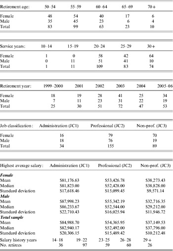
Table 1 provides descriptive statistics for the sample of 278 state university retirees under PERA. In the sample, 40.65% of retirees are male, with 34.53% retiring at age 60 or higher (10 at age 70 or older), 35.61% at the age of 55–59, and 29.86% at the age of 50–54. The sample includes a range of retirement ages, reflecting the ability of state employees to retire before the traditional age of 65. For service years, 26.62% had 30 years or more and cumulatively 95.65% had 20 years or more, and only 4.32% had 19 or fewer service years. The year of retirement varied as well with 20% retiring during 1999–2001, 47.60% during 2002–2003, and 35.61% during 2004–2006. For job classes, 12.23% had administrative positions (JC1), 55.76% professional positions (JC2), and 32.01% a non-professional employee classification (JC3).
Descriptive statistics for the sample of university retirees
Sample consists of 278 retirees (113 male and 165 female) under PERA for University of Colorado at Denver, University of Colorado at Boulder, and Metro State University.

For salary histories, 73.38% of the sample had data with no more than three missing years, with about 8.64% having missing years of seven or more. Most of the missing years were initial missing years between the hire date and the first year of recorded salary history. Missing interior years (between the first recorded salary and the retirement date) were not common (0.50 missing interior years on average) but could have been due to illness, pregnancy, family leave, and omission. For the sample, 87% had 19 or more years of salary history. The mean highest average ending salary (HAS) for retirees was $52,599.44, with the mean for the highest paid administrative group $84,988.70, for the professional class $54,365.95, and for the lowest paid clerical/custodian class $37,149.53.
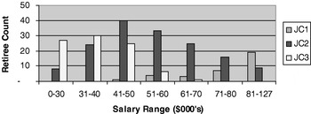
Figure 1 contains a histogram of HAS by job class, showing a wide range across the sample. The sample has considerable diversity in retirement age, gender, job class, and retirement year to examine the effect of these variables on deferred compensation.
Number of retiress by salary range and job class

3 Research methodology
This section presents the research methodology, including the inputs for calculating deferred compensation and the different measures used for deferred compensation.
Input variables
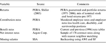
To calculate deferred compensation for PERA retirees, we used data provided by PERA, net interest rates, mortality tables, and completed salary histories. Table 2 summarizes characteristics of the input variables.
Summary of input variable characteristics

PERA provided annual rates of return for its portfolio from 1971 to 2006 and interest rates credited to member accounts from 1950 to 2006. For PERA portfolio returns prior to 1971, we used an 80/20 mix of historical nominal stock and bond returns provided by Shiller (2005). We calculated account balances for each retiree based on employee and employer contribution earnings using PERA guaranteed interest rates (AcctBalg balance) and the PERA historical portfolio returns (AcctBalr balance). The AcctBalr balance is only hypothetical as PERA does not use its own returns in calculating account balances. The AcctBalg balance is an estimate of the account balance maintained by PERA as a lump-sum alternative to monthly benefits.
PERA also provided benefit rate tables and historical contribution rates. PERA provided the current benefit rates applicable to the retirees in our sample as well as the pre-1997 benefit rates, since the Colorado State legislature substantially increased benefit rates beginning in 1997. For the historical contribution rates, we used employee and employer contribution rates contained in PERA annual reports. We adjusted the mandated employer rates by removing the parts of the contribution for health care, survivorship, and disability benefits. The adjustments were made using actuarial data in PERA annual reports. The adjustments typically reduced the employer contributions by 1–2.5%.
We used two mortality tables to calculate the expected present discounted value of the retirement benefit stream. For one mortality table, we used the Society of Actuaries (SOA) RP-2000 table (Society of Actuaries, 2000) adjusted for collar (white-collar versus blue-collar). Specifically, we adjusted the combined-healthy rates in RP-2000 Tables 4-5 and 4-6 using the white-collar adjustment ratios in RP-2000 Table 5-5. Further, we generated a dynamic, cohort mortality table for each retiree in our sample using the Mortality Projection Scale AA (RP-2000 Table 7-3) following the methodology described by Society of Actuaries Group Annuity Valuation Table Task Force (1995). Using the RP-2000 dynamic, collar-adjusted, combined-healthy rates is consistent with US Department of Treasury recommendations made by the American Academy of Actuaries (Segal, Reference Segal2001). For the second mortality table, we used the period mortality table provided to us by PERA in 2006. We generated a dynamic, cohort mortality table for each retiree using the SOA Mortality Projection Scale AA. Thus, we used two cohort mortality tables (RP-2000 and PERA) for each retiree in our sample.
In calculating the expected present discounted value of retirement benefits, we used net interest rates provided on single premium insurance annuities (SPIA). A sample of net interest rates was provided by Mr Richard Greer, F.S.A. and M.A.A.A. of Aegon Corporation. The interest rates were net of profit, commission, safety margin, and other factors. These net interest rates vary by retirement date, retirement age, and gender. Since the net interest sample did not exactly match each retiree, we used a weighted nearest neighbor search to find the best rate for each retiree. For 178 retirees, we had an exact match on retirement date, retirement age (in nearest whole year), and gender. For the 100 retirees without an exact match, the average number of days was 21 between the retirement date and date of the matching net interest rate.
For employees with incomplete salary histories, we used a backcasting method to complete salary histories. Our approach used the Average Wage Index (AWI) and Scaled Factors (SFs) developed by the US Social Security Administration (SSA). According to the SSA website (www.ssa.gov), the AWI is ‘based on compensation (wages, tips, and the like) subject to Federal income taxes, as reported by employers on Form W-2’. The AWI has been published since 1951 with details about its derivation available at the SSA website. The SFs replaced simplistic assumptions about steady workers who earn a constant percentage of the AWI. The SFs were developed using the SSA's Continuous Work History Sample (Clingman and Nichols, Reference Clingman and Nichols2004). We used the SFs for high wage earners in our backcasting method. Consistent with the approach in Spriggs and Ratner (Reference Spriggs and Ratner2005), we backcasted the earnings for a retiree in year y at age a (E a,y) using the earnings in the next higher year (E a+1,y+1) along with the AWI for years y and y+1 and the SF for ages a and a+1 as shown in (1). To eliminate effects of part-time employment, we scaled the last year of known salary history to its full-time equivalent so that all backcasted years were based on full-time work.

Backcasting was only done for years before the first year of recorded salary history. Backcasting was not done for missing interior years. For example, if the first year of recorded salary history was 1982, 1981 was the first year of backcasting even if years 1985 and 1997 were missing. Thus, no salary was recorded in missing interior years, in this case 1985 and 1997.
Since our goal was to compare the EPDV of the PERA benefit stream to the cost of equivalent SPIA contracts, we used alternative private sector mortality tables. Details, along with the impact of mortality tables and backcasting, are described in Appendix 1.
Deferred compensation measures
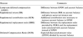
To provide robustness, we developed five measures of deferred compensation. Each measure uses the expected present discounted value (EPDV) of the retirement benefit stream. EPDV was calculated as shown in (2), consistent with the definition given by Mitchell et al. (Reference Mitchell, Poterba, Warshawsky and Brown1999). The maximum age in the RP-2000 table is 120. Table 3 provides a convenient summary of the measures. The remainder of this section provides details about each measure.
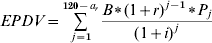
where
• a r is the age at retirement to the nearest whole year;
• B is the initial annual benefit;
• r is the benefit inflation factor (3.5% for PERA);
• P j is the probability that an individual survives for at least j years past retirement age a r – a retiree's cohort mortality table (RP-2000 or PERA) was used to calculate P j as indicated in Mitchell et al. (Reference Mitchell, Poterba, Warshawsky and Brown1999) ;
• i is the net interest rate determined using the Aegon sample of net interest rates.
Summary of deferred compensation measures

The first deferred compensation measure is the lump-sum deferred compensation defined as the difference between a member's account balance and the EPDV. We calculated this measure using account balances with alternatively PERA guaranteed rates (LSDCg) and PERA portfolio returns (LSDCr).
The second deferred compensation measure is the supplemental return on a retiree's account balance that would be necessary to achieve the EPDV during the retirement period. We calculated this measure using the Microsoft Excel IRR function with the account balance (AcctBalg or AcctBalr) as the inflow and the expected annual benefits as the outflows. The expected annual benefits were calculated using the P js derived from a cohort mortality table (RP-2000 or PERA). Then, the supplemental return is the IRR minus the net interest rate.
The third deferred compensation measure is the supplemental contribution rate during an employee's service years that would have been necessary to earn the lump-sum deferred compensation. We used two allocation approaches: a uniform rate across a retiree's service history and a weighted rate that increases linearly with service years (until 20 service years). For example, the supplemental contribution rate for a retiree in service year 1 is 1/20 times the supplemental contribution rate in service year 20. We considered 20 years of service as long-term employment. Using lump-sum deferred compensation for both PERA guaranteed and portfolio balances, we calculated four supplemental contribution rates. To calculate a contribution rate, we used the Microsoft Excel solver to search for the contribution rate that resulted in a supplemental account balance equal to the lump-sum deferred compensation. Supplemental contributions and principal earned the appropriate return (PERA guaranteed or portfolio returns) to make the future value equal to the lump-sum deferred compensation.
The fourth deferred compensation measure is the supplemental replacement ratio. We calculated the replacement ratio that a retiree would have received if benefits were based on an account balance (PERA guaranteed or portfolio returns), instead of the replacement ratio based on service years and age. To calculate an alternative replacement ratio, we used the Microsoft Excel solver to search for the initial annual benefit (B) in equation (2) with the EPDV set to the account balance. The alternative replacement ratio is the initial annual benefit divided by the retiree's highest average salary. The supplemental replacement ratio is the actual replacement ratio (typically 75%) minus the alternative replacement ratio based on the account balance.
The fifth measure is the deferred compensation ratio (DCR) equal to EPDV divided by account balance (either AcctBalg or AcctBalr). This ratio provides a relative measure for the present value of expected benefits relative to a retiree's account balance at retirement. For instance, a measure of 2.00 would indicate that a retiree would need twice the amount at retirement in his/her account balance to purchase an annuity at retirement generating similar expected future benefits.
4 Hypotheses and empirical results
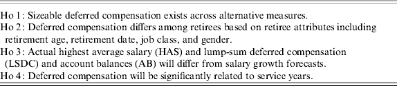
This section presents research questions and hypotheses, followed by the empirical results. The hypotheses are summarized in Table 4.
Hypotheses examined for deferred compensation
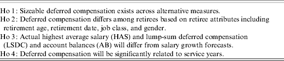
Hypotheses for deferred compensation
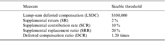
To test the primary hypothesis of sizeable deferred compensation existing for career retirees, we use the sizeable thresholds for each of the five deferred compensation measures described earlier and shown in Table 5. Each threshold was chosen to demonstrate substantial levels of deferred compensation as meaningful amounts of additional compensation to career employees.
Threshold compensation values for hypothesis testing
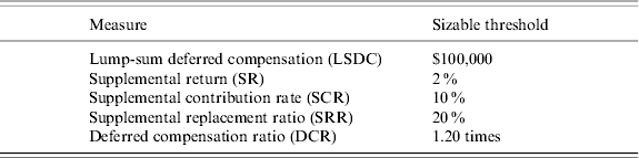
The existence of large levels of unfunded liability for PERA and other public DB plans suggests that earnings on contributions are not sufficient to provide promised benefit levels. Because career employee benefits are partially subsidized by lower benefits relative to non-career employees, deferred benefits are also expected to be substantial. We test Hypothesis 1 assuming that each retiree has a minimum of 30 service years (30+ service years), providing an initial annual benefit amount of at least 75% of HAS for each retiree in the sample. Retirees with longer than 30 years of university employment had their actual number of years of service in this model.
To better understand the relative importance of different attributes that affect the deferred compensation for individual retirees and to test Hypothesis 2, we use the following linear model (3), regressing deferred compensation against retiree attributes. As for the basic hypothesis, we used 30+years for service years.

• Y is a deferred compensation measure (deferred compensation ratio, lump-sum deferred compensation, supplemental return, supplemental replacement ratio, or supplemental contribution rate);
• RetAge is a retiree's retirement age;
• RetDateCode is the retirement period code (relative month from 1 to 96) in the retirement period (1999 to 2006);
• Gender is the indicator variable for gender.
• Admin is the indicator variable for the job classification of 1 if a retiree is in the Administrative job class, 0 otherwise.
• Prof is the indicator variable for the job classification of 1 if a retiree is in the Professional job class, 0 otherwise.
The attributes that affect levels of deferred compensation are retirement age, the historical period of retirement, gender, and job class. Retirement age (RetAge) is an important measure of retirement benefit generosity as most employees prefer to retire at a younger age. Retiring at a younger age leads to a longer period in retirement to receive benefits. A negative relationship between retirement age and deferred compensation would be expected, since EPDV increases as retirement age decreases, consistent with the view of recent ballot proposals that a higher mandated retirement age will reduce pension benefit costs. Because most retirees had 30 service years, a lower retirement age should not be offset by a lower initial benefit level due to fewer service years. We postulate a linear relationship because mortality should increase proportionally over most of the range of retirement ages in our sample.
Retirement period (RetDateCode) encodes the movement of net interest rates and PERA portfolio returns in the period of our study (1999–2006). We expect deferred compensation to increase in periods of low stock returns and bond rates, since retirees would not be able to earn as much on contributions during these periods to build up retirement accounts. PERA portfolio returns impact the account balance with PERA portfolio returns as well. Net interest rates directly impact EPDV as shown in (2). Since stock returns and bond rates followed a similar pattern in the period of our study, we use a single variable instead of two variables to reduce the model complexity without sacrificing the model's explanatory power. We postulate a linear relationship because interest rates declined proportionally during the retirement period in the sample. However, in different retirement periods, there is no reason why a linear relationship would be appropriate.
Gender and the job classification variables (Admin and Prof) are indicator variables in the model. For the job classification variables, the non-professional, clerical job class is the omitted variable for comparison. Because of longer longevity for females, the EPDV for a female retiree would be expected to be larger than a male retiree, holding other factors constant. Since we could not use a repeated measures design on gender, the gender effect may be diluted by other factors, such as salary growth, part-time work, and leaves of absence. For job classification, we expected to see an ordering of administrative (JC1), professional (JC2), and non-professional (JC3), consistent with the average HAS values in Table 1. As noted in Table 1, the mean for deferred compensation was much higher for the administrative class, followed by the professional, and then the non-professional class. Some state governments including Colorado have recently not allowed new administrators to be under state DB plans to attempt to reduce pension costs for this reason. We also check for the significance of interaction of gender and job classification to see if longer mortality for females had a larger impact than possible factors favoring males, such as higher salary growth, fewer leaves of absence, and less part-time work.
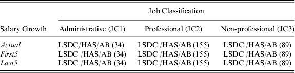
Salary growth is another retiree characteristic that impacts DB pension benefit levels. Hypothesis 3 determines if actual salary growth rates are similar to growth rates used in traditional wage – earning profiles. We also assess the impact of salary growth close to retirement. To study the effect of salary growth, we used three single factor models (shown in Table 6) with salary growth as the factor and deferred compensation (DC), account balance (AB), and highest average salary (HAS) as dependent variables. We use both account balance and deferred compensation because HAS changes and account balance changes could cancel deferred compensation changes. We test separate models for each job classification. We expected salary growth to have a more significant impact on the two higher job classes, since these classes have a greater opportunity for salary growth.
Salary growth model
(dependent variables and sample sizes noted in cells)
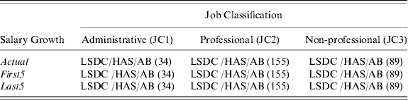
In the salary growth models, we compare actual salary histories (control level) collected from personnel rosters and backcasting to forecasted salary histories constructed from a base part and a forecasted part. As in model (3), the total service years are constant in the salary histories with a minimum of 30 years of earned service for each retiree (30+). The base part consisted of a mix of backcasted salaries and actual salaries. For the forecasted part, the First5 approach forecasts salaries after the first five years of actual salary history. The Last5 approach forecasts only the last five years of salary history. In both approaches, forecasting is done using the highest salary computed with the combined AWI and SF (equation (1)) or the AWI alone by eliminating the SF ratio in (1). Using the AWI alone provides higher salary growth after age 50. Since salaries in public employment seldom decline,Footnote 7 the AWI may provide a better estimate of salary growth for older employees than both AWI and SF.
The final hypothesis predicts that deferred compensation is related to service years. In the other models, service years were set to the minimum of 30 or the reported university working period (retirement date minus hire date). Service years are interesting to analyze because benefit rates are determined by a combination of service years and retirement age. At the earliest retirement age (50), PERA monthly benefits begin with 25 years of service. At age 55, monthly benefits begin with 20 years of service. An employee reaching these minimum thresholds has the option to continue working or retire with reduced benefit levels. Although it is beyond the scope of this paper to provide a definitive answer to this decision problem, we wanted to provide some insights using our sample. To test this hypothesis we use the following model

• Y is a deferred compensation measure (ratio of present value of future benefits to retirement account balance, lump-sum deferred compensation, supplemental return, supplemental replacement ratio, or supplemental contribution rate);
• RetAge is the retirement age;
• Service is the number of service years.
We isolate the effects of service years and retirement age in (4). Service years were controlled in the sample by choosing a number of service years and then backcasting to achieve the specified service years. Since retirement age did not change for individual retirees, interaction between retirement age and service years was not studied. In cases in which an individual has more actual years of salary history than the specified service years, we truncated the known salary history. To provide a range of service years consistent with the retirement age of the observations in the sample, we used two samples. For the entire sample, we varied the service years from 25 to 30 to be consistent with retirees with a retirement age less than 55. To provide a broader range of service years, we varied service years from 20 to 35 for retirees with a retirement age greater than or equal to 55.
Empirical results and analysis
The empirical results for each hypothesis are discussed in the subsections below including the results deferred compensation measures and cross-sectional results.
Deferred compensation
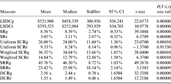
Substantial deferred compensation was confirmed in all but one deferred compensation measure as listed in Table 7. The t-tests in Table 7 were conducted using the thresholds in Table 5 with the full retiree data set (sample size of 278). We performed the same analysis using the cohort RP2000 mortality table with similar results. The hypothesis for the uniform supplemental contribution rate using PERA portfolio returns (SCRr) was not rejected with a mean difference of 10%. However, the confidence interval indicates that the hypothesis would have been rejected with a mean difference of 8.5%. The other confidence intervals are far away from the thresholds in Table 5, so we have strong evidence that mean deferred compensation values are substantial.
Hypothesis 1: t-test results for 30+service years with Cohort PERA mortality table

Interpreting the results, a retiree in the sample on average would have to pay an additional $521,908 for a private annuity at retirement to be able to generate similar expected retirement benefits, based on contributions earning a guaranteed rate over the average salary history, or make a 8.58% supplemental return over guaranteed rates, or receive 26% more in compensation for each working year, or have on average 2.5 times as much at retirement earnings in an account balance. Hence, deferred compensation is substantial.
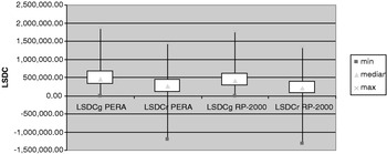
To explore further, we summarized the distribution of lump-sum deferred compensation for combinations of account balance (LSDCg for PERA guaranteed rates and LSDCr for portfolio returns) and mortality table (PERA cohort and RP-2000 cohort). The box charts in Figure 2 show that most retirees received retirement benefits substantially larger than their account balances for both guaranteed and portfolio returns. For the portfolio return balance with the PERA mortality table (LSDCr PERA), only six retirees had a balance less than −$100,000, whereas 55 had a balance in excess of $500,000. The minimum point in each box chart is for a retiree who retired at age 76 after working 51 years. The minimum deferred compensation for PERA guaranteed account balances is 0 because PERA uses the account balance as a floor. In this case, the retiree could receive the account balance as a lump-sum payment or receive monthly benefits based on the guaranteed account balance with an 8.5% annuity rate.
Box charts of lump-sum deferred compensation

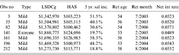
Identification of outliers provides insights about the characteristics of retirees who earned large amounts of deferred compensation. Table 8 below lists the mild outliers (third quartile plus 1.5 times the inter quartile range) and extreme outliers (third quartile plus 3 times the inter quartile range). Each outlier was an administrative employee with a HAS greater than $100,000, with LSDC greater than $1 million. All outliers except one had an early retirement age around the mid 50s. Net interest rates were important parts of most outliers as the retirement dates involved relatively modest rates in the 5% range. Five of seven outliers had substantial salary increases in their last five years. In each case, there was one year with a substantial salary increase greater than 18%.
LSDCg outliers for the cohort PERA mortality table

Relative effect of different attributes on deferred compensation
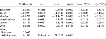
Table 9 shows the regression results with DCRg as the dependent variable in the attribute regression model. Using other measures of deferred compensation we found similar results. The adjusted R-square indicates a good fit for the regression. As expected all variables are significant. For Gender and RetAge the coefficients are negative. Holding other factors constant, retirees that retire earlier receive significantly high compensation, with the largest t-statistic in the model on RetAge. Women also receive significantly higher relative deferred compensation, associated with longer longevity in retirement. The coefficients on RetDateCode, Admin, and Prof are positive. Retirees retiring in later months for the sample had higher relative deferred compensation. This result suggests that the decline of the stock market in 2001 and the decline in interest rates starting in 2002 increased deferred compensation because EPDV increases as earnings on contributions decrease, and, hence, retirement account balances decrease. For the job class variables, with the non-professional job class as the omitted class, both the Admin and Prof classes had significantly higher relative deferred compensation than non-professionals, with a larger coefficient and t-statistic for the Admin class. We also performed regressions with interaction variables on gender and job class. Because the interaction variables between gender and job class were not significant, gender within classes does not seem to affect deferred compensation.
Deferred compensation ratio (DCRg) regressed against retiree characteristics

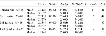
As a sensitivity test, we performed a quartile analysis shown in Table 10. For the top quartile of the deferred compensation ratio, the mean DCRg is 3.51, and about 37% of retirees in this quartile are male, with an average retirement age of 54. Retirees in the top quartile on average retired in later months (about month 64), and about 81% were administrative or professionals. In the bottom quartile, the mean DCRg ratio is 1.77, and approximately 48.57% of retirees are male. The bottom quartile also had a much higher average retirement age of 63 years, a much earlier retirement date code (about 42), and a much smaller percentage of administrators and professionals (49%), including only four retirees from the administrative class. We also performed regressions for each of the individual quartiles, with similar results to the overall regression as a sensitivity check. Within the quartiles, gender and job class became a less significant variable. Otherwise, regressions results were similar, with again RetAge having the largest t-value.Footnote 8
Descriptive statistics for deferred compensation ratio (DCRg) by quartiles
Gender indicates the fraction of male retirees. RetDateCode indicates the retirement month in the range 0 to 84.

To test the model complexity, we performed the sample regressions using non-linear forms for the variables. Tests indicated insignificance for squared and cubed forms of independent variables, and a better fit for the linear versus a log or other non-linear models. Thus, the simpler linear model provides a better explanation for the sample data than a more complex model.
Salary growth analysis
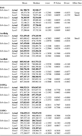
We used a collection of single-factor ANOVAs (one per job class) to test the impact of salary growth on HAS, deferred compensation (LSDCg and LCDCr), and on retirement account balances (AcctBalg and AcctBalr). ANOVA result F-statistics indicted a significant difference at a p-value of 0.00343 for HAS, among actual and forecast values, so we performed post hoc paired t-tests for salary growth pairs, to test for significant differences between actual salary growth and salary growth First5 (forecasts after first five years of actual salary history) and Last5 (forecasts for last five years of service only). We continued to use an alpha level of 0.05 for paired t-tests, resulting in a family-wise error rate of 0.0975 using the Bonferroni error correction (Sidak, 1967). Cohen's (Reference Cohen1977) d-tests are used to test the strength of effects with significant effect size cutoffs, listed with the results in Table 11.
Paired t-tests are for difference between actual and forecast values using First5 and Last5 forecasts
P-values indicate significant levels for the paired t-tests for forecast less actual value. Cohen's D- test statistics indicates a significant effect size where ⩾0.2=a small effect, ⩾0.5=medium, and 0.8=a large effect size.

The t-test results indicate significant differences between actual and forecasted means for HAS, AcctBalg, and AcctBalr for both forecasts, as well as LSDCg and LSDCr for the last five forecasts for Job Class 1 (administrative) and Job Class 2 (professional), but no significant differences for Job Class 3 (non-professional). Actual values were greater than forecasted values, although effect sizes were large only for HAS with Job Class 1. The results were robust across alternative deferred compensation measures and mortality tables, suggesting that caution is needed when studies rely on forecasted salaries for more highly compensated public sector employees. Although forecasted salary growth rates and deferred compensation appear to be underestimated, forecasted salaries demonstrate little bias for lower-paid public employees. The results have two limitations: (1) they do not indicate if forecasting without an initial salary history will provide realistic estimates of salary growth; and (2) they do not address wage growth differences due to part-time work or workforce leaves since forecasted salaries had the same work status as the original salaries.
Service years
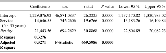
Table 12 shows the results of regressing the lump-sum deferred compensation for PERA guaranteed rates (LSDCg) against service years and age with service years varying from 20 to 35 years. We did similar regressions for other deferred compensation measures and varying the service years from 25 to 30 years, with similar results. LSDC increases as the service year's rise, with a positive, significant coefficient on service years.
LSDCg regression against service years 20–35 and retirement age
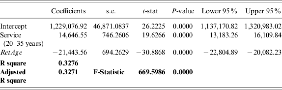
Holding other factors constant, retirees appear to gain greater lump-sum deferred compensation as they increase their service years. Consistent with previous results, however, LSDC goes down the older the age of a retiree at retirement, with fewer future benefits provided with a lower remaining life span for older retirees. In actual situations, service years cannot increase without increases in age so it is not clear that working beyond some threshold (such as 30 service years) is worthwhile.
Discussion and additional analysis
Most comparative studies use unadjusted returns to compare DB and DC plans, although risk considerations are used in determining optimal plan selection. The results in this study confirm the importance of risk in comparing DB and DC plans. The retirees in this sample were shielded from the effects of the stock market decline and low bond rates in a substantial part of the study period. If retirement assets had been subject to stock and bond market risks, many of the retirees would likely have had to change their retirement plans in some way.
To adjust for risk, we emphasized PERA guaranteed rates as a baseline. Retirement benefits above the baseline were considered as deferred compensation due to the risk-free nature of the benefits. PERA guaranteed interest rates were substantially above traditional guaranteed interest rates, such as the 90 day Treasury bill rate during the period of this study. Without assuming any investment risk, career employees received returns substantially in excess of the returns available with the PERA portfolio returns. The results for the supplemental contribution rates show that usage of the employer contribution rate in a total compensation model substantially understates the compensation value of PERA pension benefits.
Another way to adjust for risk is to use risk-adjusted returns. Since there is no standard risk-adjusted return measure for DB plans, we devised two alternative measures (equations (5) and (6)) that are simple variations of the Sharpe ratio (Sharpe, Reference Sharpe1994) and Sortino ratio (Sortino and Price, Reference Sortino and Price1994). We used IRRs instead of annualized returns because DB plans do not provide annual returns. Since there is no clear choice for risk adjustment of DB plans, we used the standard deviation of a risk-free asset (annual 90 day T-Bill rates) and the downside deviation of PERA guaranteed rates as compared to the risk-free rate of return. Using standard deviation as a denominator (RAR sd), the risk-adjusted return of PERA DB benefits was on the average 5.9 times higher than the risk-adjusted return of a stock portfolio. Using downside deviation as a denominator (RAR dd), the risk-adjusted return of PERA DB benefits was on the average 4.6 times higher than the risk-adjusted return of a stock portfolio. Both measures demonstrate the clear superiority of risk-free DB plan benefits compared to risky DC plan benefits.
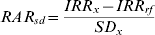
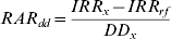
• IRR x is the internal rate of return of x (stock, bond, risk-free, or PERA DB) with contributions as inflows and the account balance as a single outflow – or PERA DB, we used the EPDV as the single outflow;
• SD x is the standard deviation of returns of x (stock, bond, or PERA DB). For PERA DB, we used the standard deviation of the risk-free asset;
• DD x is the downside deviation of returns of x (stock, bond, or PERA DB) using the risk-free rate as the minimum acceptable return – for PERA DB, we used guaranteed rates in the downside deviation calculation.
This study also indicates the lack of attention to the benefit/deferred compensation side of public DB plans in contrast to a great deal of attention on the cost side of financing benefits in most public policy debate. Because DB plans provide substantial compensation beyond employer contribution costs, total compensation models should use a more precise estimate of deferred compensation value under DB plans for career employees. We are unaware of other studies that have estimated or calculated the implicit value of deferred compensation for public DB plan benefits.
5 Concluding remarks
This paper emphasizes the benefit side of DB plans, estimating the value of deferred compensation for career university employees under the Colorado Public Employees Retirement Association (PERA) plan. Deferred compensation is derived from the difference between the expected present discounted value of promised retirement benefits and the earnings that would historically be made on contributions until retirement. Deferred compensation was estimated using a unique data set of salary histories. To improve estimates of deferred compensation, we augmented the data set with backcasted salary histories for missing data and net interest rates from the Single Premium Insurance Annuity marketplace.
We find evidence of considerable lump-sum deferred compensation that is on average significantly larger than a $100,000 threshold, with a mean of $521,908 based on contributions earning at guaranteed rate. For the alternative measures, we similarly find evidence of considerable average deferred compensation, with confidence intervals for each deferred compensation measure indicating much higher values than the levels in the hypothesis tests. Empirical cross-sectional results in general indicate that women, higher-paid administrators and professionals, employees with service somewhat exceeding minimum service year requirements, younger retirees, and those retiring in periods of stock market decline and low interest rates, receive higher levels of deferred compensation. In contrast, retirees that retired at older ages, and, hence, had lower longevity in retirement, receive lower deferred compensation. Outlier tests revealed higher-paid administrative employees with $100,000 or highest average salaries or more had levels of lump-sum deferred compensation of $1 million or greater.
The results indicate significant deferred compensation that should be recognized in more precise total compensation models for long-term employees. In addition to being able to attract talented career employees, with large government employee retirements expected in the next decade, deferred compensation has implications for job performance, hiring/retention effort, organizational learning, customer service, and cost control. The results also provide insights for employees deciding between a DB versus a DC plan and job changes involving loss of a DB plan, as well as identifying factors that have a significant effect on deferred compensation costs and, hence, funding issues.
For future research utilizing this data set, we plan to study the impact of service credit purchases on deferred compensation and the impact of deferred compensation on job changes from a public DB plan to a DC plan. We would also like to collect additional data to extend the scope of this research to other areas of public employment, such as K-12 education and law enforcement.
Appendix I: Impact of mortality tables and backcasting
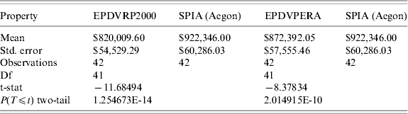
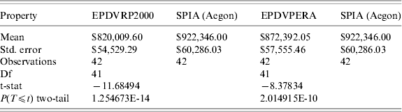
Since our goal was to compare the EPDV of the PERA benefit stream to the cost of equivalent SPIA contracts, we wanted to use private sector mortality tables. Based on previous studies (Brown et al., Reference Brown2000 and Mitchell and McCarthy 2002), we felt that private sector mortality tables would have more adverse selection than the cohort RP-2000 and PERA tables. Because we were unable to obtain a private sector mortality table, we made a comparison of the EPDV computed with the cohort RP-2000 and PERA tables to private sector SPIA contract values. Mr Richard Greer of Aegon Corporation provided a sample of 42 contract values for a subset of our sample. In the comparison, the net interest rates were identical in our EPDV calculations and the SPIA contract values. Thus, the mortality table was the only difference between the EPDV calculation and SPIA contract value. As we suspected, the private sector mortality table demonstrated more adverse selection as depicted in Table A1. On average, the SPIA contract values were 12.5% higher than the RP-2000 EPDVs and 5.7% higher than the PERA EPDVs.
Paired t-test results for mortality table impact on EPDV
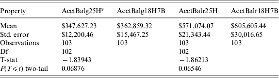
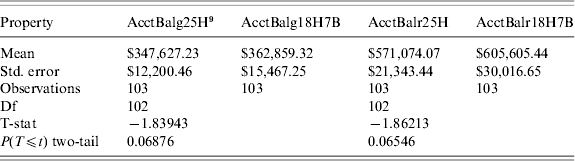
We also investigated the impact of backcasting on account balances to determine possible bias due to backcasting. Note that backcasting does not impact the HAS and EPDV calculations. For retirees with 25 years of salary history (sample size 103), we replaced part of the salary history (first seven years) with backcasted salaries. Because most of our analysis used 30 years of service with a median of 23 years of salary history, seven was the median number of backcasted years. We compared the account balances (PERA guaranteed and portfolio returns) derived from the full known salary history to the account balances derived from the augmented salary history (actual history along with salary history replaced by backcasting). As shown in Table A2, the t-test results indicated weak evidence (significant at the 0.10 level) of bias in which the average balances derived from mixed salary data were about 4.5% larger than the balances derived from actual salary history.
The impacts of mortality table and backcasting indicated that our methodology likely understates deferred compensation. The usage of a private sector mortality table would likely provide a small increase (5% to 10%) to EPDVs. Usage of full salary history may provide a small decrease to account balances and a corresponding small increase to deferred compensation; however, the statistical results were not conclusive to make this statement with reasonable confidence.
Paired t-test results for backcasting impact on account balances