2.1. Numerical set-up: direct numerical simulation of a single bubble in homogeneous and isotropic turbulent flow

We perform direct numerical simulations of an incompressible gas bubble immersed in a homogeneous and isotropic turbulent flow of an incompressible liquid, using the open-source software Basilisk (http://basilisk.fr) (Popinet Reference Popinet2003, Reference Popinet2009; Abu-Al-Saud, Popinet & Tchelepi Reference Abu-Al-Saud, Popinet and Tchelepi2018). Density and dynamic viscosity ratios are set to $850$ and $25$, respectively, close to water–air ratios (830 and 58 respectively). The simulation goes in two steps. We first create a homogeneous isotropic turbulent flow by solving the one-phase incompressible Navier–Stokes equations with an additional forcing term proportional to the velocity (Rosales & Meneveau Reference Rosales and Meneveau2005). After a transient regime, the flow reaches a statistically stationary homogeneous and isotropic turbulent state. The turbulent fluctuations are characterized by the Taylor Reynolds number $\textit {Re}_\lambda$, defined at the correlation length of the velocity gradients, namely the Taylor micro-scale $\lambda _T = \sqrt {15\nu / \epsilon }\, u_{rms}$ Pope (Reference Pope2000), where $u_{rms}$ is the root mean square of the velocity. The Taylor Reynolds number of the flow is $\textit {Re}_\lambda = u_{rms}\lambda _T/\nu = 55$. In physical units, assuming $\epsilon = 1\ {\rm m}^2\ {\rm s}^{-3}$, in water, we would have $u_{rms} = 0.12\ {\rm m}\ {\rm s}^{-1}$ and $\lambda _T = 0.46$ mm. We then extract snapshots of the flow and use them as flow initial conditions for bubble injection. At the bubble scale, flow structures are correlated on a typical time scale $t_c(d) =\epsilon ^{-1/3}d^{2/3}$, called the eddy turnover time. To make sure the initial conditions are independent, we take flow snapshots separated by at least $6 \, t_c$. The spherical bubble is injected at the centre of the simulation box by changing locally the density and viscosity. The bubble size is chosen so that it lies within the inertial range of the turbulent cascade where the flow is scale invariant. The bubble diameter to box length ratio is $0.13$. During this second stage, forcing is maintained to sustain turbulence, but only in the liquid phase to guarantee that bubble deformations only come from the fluid forcing. In both steps, we use adaptive mesh grid refinement in order to save computational time while resolving all the physical length scales of the problem. The minimum grid size corresponds to 34 points per bubble radius. Details of the numerical set-up as well as a convergence study can be found in Rivière et al. (Reference Rivière, Mostert, Perrard and Deike2021).

In this study we keep the Taylor Reynolds number constant and we vary the bubble Weber number by changing the value of the surface tension coefficient. The bubble Reynolds number is $\textit {Re}(d) = 124$. Assuming $\epsilon = 1\ {\rm m}^2\ {\rm s}^{-3}$, this Reynolds would correspond to a bubble of size $d=0.9$ mm. We explore eight values of $\textit {We}$ ranging from $\textit {We}_c \approx 3$ to $0.1\textit {We}_c$. For each Weber number, we run between 3 and 5 simulations. Except when the bubble breaks (at $\textit {We}=2.9$), we run every simulation for at least $20\, t_c$, so that the total time per ensemble is approximately $100\, t_c$. Table 1 summarizes the exact number of simulations and total computational time per Weber number we perform.

Table 1.

Number of simulations and total simulated time per value of the Weber number.

2.2. Modes of deformations

To quantify bubble deformations, we decompose the local bubble radius $R$ into the real spherical harmonic base $Y_{\ell }^m(\theta, \phi )$, where $\ell$ and $m$ are the principal and secondary numbers respectively, and $\theta$ and $\phi$ the co-latitude and longitude,

(2.1)\begin{equation} R(\theta, \phi, t) = R_0\left[1 + \sum_{\ell=2}^{\infty} \sum_{m=-\ell}^\ell x_{\ell, m}(t)Y_\ell^m(\theta, \phi)\right], \end{equation}

and we track the modes’ amplitude $x_{\ell, m}$ over time. Bubble shape is described in the bubble frame of reference so that all harmonics $\ell = 1$, corresponding to bubble translation, are null by definition. Numerically, the bubble centre is determined at each time step recursively by moving the frame origin to minimize the amplitudes of all modes $\ell =1$. The recursion stops when the centre displacement between two steps is less than $2.5\times 10^{-6}R_0$. This condition ensures that $|x_{1, m}|<4 \times 10^{-6}$ for all values of $m$. Note that the spherical harmonic decomposition holds as long as the local radius $R$ is mono-valued. The procedure to compute the spherical harmonics is described in detail in Perrard et al. (Reference Perrard, Rivière, Mostert and Deike2021).

Figure 1 shows two typical temporal evolutions for the mode $(\ell, m) = (2, 0)$, at two different Weber numbers. Time is made dimensionless using the Rayleigh frequency $f_2^q$. For both $We$, we observe random oscillations around zero and the predominance of the bubble resonant frequency $f_2^q$. The amplitude of the oscillations increases with $We$.

Figure 1.

Typical temporal evolution for the mode $(2, 0)$ at two different Weber numbers. Time is made dimensionless using the Rayleigh frequency $f_2^q$. Modes exhibit random oscillations, with an amplitude that is increasing with $\textit {We}$.

Since we do not prescribe any special orientation relative to the bubble shape, all modes with the same principal number $\ell$ are statistically equivalent. Indeed, one can verify that a rotation of a mode can be expressed as a linear combination of all the other modes with the same principal number. As a consequence, we omit $m$ in what follows. For instance, $x_\ell (t)$ represents a typical temporal evolution of one of the modes $\ell$. In addition, assuming that $x_{\ell, m}$ are independent, the ensemble averaging operation $\langle \cdot \rangle$ is computed over different simulations and over the $m$ values for a given $\ell$. Roa et al. (Reference Roa, Renoult, Dumouchel and Brändle de Motta2023) used a reference frame dynamically oriented with the bubble principal axis of deformations. In practice, their reference frame maximizes the amplitude of mode $(2,0)$, such that the differential elongation can be studied as the invariance by rotation is broken.

3.1. Model: a stochastic linear oscillator

Following Risso & Fabre (Reference Risso and Fabre1998), we introduce a linear stochastic model to describe each mode's dynamics

(3.1)\begin{equation} \ddot{x}_{\ell} + \varLambda_\ell(\textit{We}) \dot{x}_\ell + \varOmega_\ell(\textit{We})^2 x_\ell = \mathcal{T}_\ell(\textit{We}, t), \end{equation}

where $\varLambda _\ell$ and $\varOmega _\ell$ are the damping rate and natural frequency, respectively, and $\mathcal {T}_\ell$ is a random variable which models the turbulent forcing. In this section, we aim at measuring $\varLambda _\ell$, $\varOmega _\ell$ and the statistical properties of $\mathcal {T}_\ell$ from the deformation dynamics. Note that $\varLambda _\ell$, $\varOmega _\ell$ and $\mathcal {T}_\ell$ may also depend, in general, on the Reynolds number at the bubble scale. However, here, we keep the bubble Reynolds number fixed and investigate the dependency of $\varOmega_\ell$, $\varLambda_\ell$ and $\mathcal{T}_\ell$ on the Weber number $We$. Conversely to what other authors have done, time is made dimensionless using the eddy turnover time at the bubble scale $t_c(d) = \epsilon ^{-1/3}d^{2/3}$ and, from now on, $\dot {\cdot }$ denotes derivatives with respect to this dimensionless time. This choice avoids a priori the need to have a forcing term depending on bubble properties such as surface tension. It decorrelates the turbulent forcing (right-hand side), from the bubble response (the left-hand side). In these units, the Rayleigh frequency and the Lamb damping rate write $(\varOmega _\ell ^q)^2 = 16(\ell -1)(\ell + 1)(\ell +2)/\textit {We}$ and $\varLambda _\ell ^q = 8 \sqrt {2}(\ell + 2)(2 \ell +1) \textit {Re}(d)^{-1}$, respectively. Note that, in this study, we have not varied the eddy turnover time. When the bubble size lies within the inertial range of the turbulent cascade its dynamics is primarily controlled by inertial effects, and the parameters may not depend explicitly on the bubble Reynolds number, as long as $\textit {Re}(d) \gg 1$.

In order to measure the coefficients and the force statistics of (3.1), we make the following assumptions:

1. (H1) The modes’ dynamics is linear and uncoupled, which is valid for $x_\ell \ll 1$, corresponding to $\textit {We}\ll 1$.

2. (H2) The bubble deformation is one way-coupled to the flow. This hypothesis is discussed in § 3.5.

3. (H3) The forcing $\mathcal {T}_\ell$ is statistically stationary.

4. (H4) The damping rate and the natural frequency do not depend on time.

From hypothesis (H2) the effective $\mathcal {T}_\ell$, in units of the eddy turnover time, is independent of $\textit {We}$. From hypothesis (H3), the effective forcing is completely determined by its auto-correlation function (or equivalently its spectrum), and its probability distribution function (p.d.f.).

Under these hypotheses, in the next sections, we will show that

1. (i) The natural frequency is not modified by the presence of the flow: $\varOmega _\ell = \varOmega _\ell ^q$.

2. (ii) There is an effective viscosity, driven by turbulence, so that $\varLambda _\ell =0.6 (\ell + 2) (2\ell + 1)$ for $\textit {Re}(d)=124$.

Combining (i), (ii) and (3.1) we will deduce the statistical properties of the forcing $\mathcal {T}_\ell$.

3.2. Frequency response of the oscillator – amplitude of the Fourier transform

To rationalize the qualitative observations of figure 1 and identify the angular frequency $\varOmega _\ell$, we investigate the frequency response of the bubble. To do so, we compute the temporal Fourier transform, $\hat {x}_\ell$ of $x_\ell$ for all $\ell$ and $\textit {We}$

(3.2)\begin{equation} \hat{x}_\ell(\varOmega) = \frac{1}{T}\int_{0}^T x(t){\rm e}^{-{\rm i}\varOmega t} {\rm d}t, \end{equation}

where $\hat {x}_\ell$ is also a random variable, $T$ is the duration of the time signal and $\varOmega$ is the angular frequency. Similarly, we introduce $\hat {\mathcal {T}}_\ell$, the Fourier transform of the effective forcing

(3.3)\begin{equation} \hat{\mathcal{T}}_\ell(\varOmega) = \frac{1}{T}\int_{0}^T \mathcal{T}(t){\rm e}^{-{\rm i}\varOmega t} {\rm d}t. \end{equation}

Figure 2 shows the ensemble average $\langle |\hat {x}_\ell | \rangle$ as a function of the angular frequency $\varOmega$, normalized by the corresponding Rayleigh natural frequency $\varOmega _\ell ^q$.

Figure 2.

Amplitude of the modes’ Fourier transform for all $We$ as a function of the frequency normalized by the corresponding Rayleigh frequency. The Weber number value is colour coded.

For $\varOmega <\varOmega _\ell ^q$, for every $\textit {We}$, $\langle |\hat {x}_\ell | \rangle$ is approximately constant. The low-frequency dynamics is similar to that of a white noise.

At $\varOmega =\varOmega _\ell ^q$ (back dotted line), for $\textit {We}\leq 0.46$ we observe a peak that resembles the resonant response of an oscillator at its natural frequency. This peak does not exist for larger values of $We$. Nevertheless, for every $\ell$, we observe a transition at this very frequency.

For $\varOmega >\varOmega _\ell ^q$, at all $We$, we report a sharp power-law decay, following at least $(\varOmega /\varOmega _\ell ^q)^{-4}$.

Finally, for $\varOmega > 3\varOmega _\ell ^q$, the spectrum amplitude is below the noise level. Note that this part also corresponds to the end of the inertial range.

Dimensional measurements of bubble deformation dynamics were performed by Ravelet et al. (Reference Ravelet, Colin and Risso2011) in the context of bubbles rising in turbulence. They measured the temporal spectrum of the horizontal bubble main axis, a proxy for the amplitude of the second Rayleigh mode. The overall shape of their power spectrum was similar: weak variation for $\varOmega <\varOmega _\ell ^q$, no resonance at $\varOmega _2^q$ and a strong decay for $\varOmega >\varOmega _\ell ^q$. In the absence of gravity, Risso & Fabre (Reference Risso and Fabre1998) also reported a transition at $\varOmega _2^q$, with a rapid decay for $\varOmega >\varOmega _\ell ^q$ of the projected area spectrum.

The cutoff frequency being $\varOmega _\ell ^q$ for all considered cases, we deduce that the bubble natural frequency in turbulence, $\varOmega _\ell$ of (3.1), is not modified by the presence of the surrounding turbulent flow and that

(3.4)\begin{equation} \varOmega_\ell = \varOmega_\ell^q = 4 \left [\frac{(\ell -1)(\ell + 1)(\ell +2)}{\textit{We}}\right ]^{1/2}. \end{equation}

It is surprising that the bubble natural frequency remains unchanged. Indeed, Prosperetti (Reference Prosperetti1980) showed, for a bubble in an initially quiescent flow, that viscous effects induce an additional memory term in the bubble dynamics. This memory term can be modelled by an effective natural frequency and damping term. The surrounding flow field can also modify the natural frequency. In a uniaxial straining flow for instance, Kang & Leal (Reference Kang and Leal1988) demonstrated that a coupling between modes $\ell =2$ and $\ell =4$ decreases the mode 2 natural frequency at linear order, with a corrective term linear in $We$. We hypothesize that the stochastic nature of turbulence cancels, on average, these contributions. In the following, we use the theoretical expression of $\varOmega _\ell ^q$, for the bubble natural frequency, $\varOmega _\ell$.

3.3. Zero frequency limit and $We$-dependency of the forcing

In this section, we investigate the zero frequency limit, and discuss the consequence for the We-dependency of the forcing. By computing the Fourier transform of (3.1), combined with (3.4), we obtain an expression linking $\hat {x}_\ell$ and $\hat {\mathcal {T}}_\ell$

(3.5)\begin{equation} |\hat{x}_\ell|(\textit{We}, \varOmega) = \frac{|\widehat{\mathcal{T}}_\ell|(\textit{We}, \varOmega)}{\sqrt{(\varOmega^2 - \varOmega_\ell^q(\textit{We})^2)^2 + \varLambda_\ell(\textit{We})^2 \varOmega^2}}. \end{equation}

The spectral behaviour of each $x_\ell$ is a combination of the forcing spectrum $\hat {\mathcal {T}}_\ell$ and the bubble response. In the limit case $\varOmega =0$, using the expression of the bubble natural frequency (3.4), we have

(3.6)\begin{equation} |\hat{x}_\ell|(\textit{We}, 0) = \frac{|\hat{\mathcal{T}}_\ell|(\textit{We}, 0)}{\varOmega^q_\ell(\textit{We})^2}= \frac{\textit{We}}{16(\ell -1)(\ell + 1)(\ell +2)} |\hat{\mathcal{T}}_\ell|(\textit{We}, 0). \end{equation}

We can use this expression to investigate the $We$-dependency and $\ell$-dependency of $\hat {\mathcal {T}}_\ell$ at $\varOmega =0$. We extract $\langle |\hat {x}_\ell |\rangle (\textit {We}, 0)$ by averaging $\langle |\hat {x}_\ell | \rangle (\textit {We}, \varOmega )$ over the range $5\times 10^{-3}<\varOmega /\varOmega ^q_\ell <10^{-1}$ where the spectrum is constant.

Figure 3(a) shows $\langle |\hat {x}_\ell |\rangle (\textit {We}, 0)$ as a function of $\textit {We}$. Solid lines of slope 1 are superimposed, showing that $\langle |\hat {x}_\ell |\rangle (\textit {We}, 0)$ increases linearly with $\textit {We}$ for $\ell <4$, up to $\textit {We} = 2.9 \approx \textit {We}_c$, when nonlinear effects start to be important. For $\ell \geq 4$, the increase is faster than linear. This effect might originate from nonlinear coupling with lower-order modes. It follows from (3.6) that $\langle |\hat {\mathcal {T}}_\ell |\rangle (\textit {We}, 0)$ is independent of $\textit {We}$ for $\ell <4$, the most energetic modes. This result justifies that the effective forcing from turbulence does not depend on the bubble deformability at low frequency. The modification of the flow induced by bubble oscillations does not impinge back on the bubble dynamics. A similar phenomenon has been observed for drops by Vela-Martín & Avila (Reference Vela-Martín and Avila2021). They investigated the interfacial stress generated by eddies depending on their distance from the interface. They concluded that eddies further that $0.2d$ from the drop interface (outer eddies) generate most of the stress. They reported that these contributions are, in addition, independent of $We$, as these eddies are too far from the interface to be affected by drop deformations. We can assume that a similar mechanism may hold also for the bubble dynamics so that $\hat {\mathcal {T}}_\ell$ does not depend on $\textit {We}$ either, at least for $\ell <4$. These results justify hypothesis (H2) at low frequency, and we assume that (H2) holds for all frequencies. From now on, we therefore assume that $\mathcal {T}_\ell$ does not depend on $We$. This hypothesis will be further validated and tested in § 3.5. The zero frequency limit also depends on the mode order $\ell$. Figure 3(b) shows the compensated spectrum limit $\langle | \hat {x}_\ell | \rangle (\varOmega =0)/ \textit {We}$ as a function of $\ell$. We find that the zero frequency limit decreases slightly faster than $(\varOmega ^q_\ell )^{-2} \sim [(\ell -1)(\ell +1)(\ell +2)]^{-1}$ of (3.6) (red line). It suggests that $|\hat {\mathcal {T}}_\ell |$ weakly decreases with $\ell$, with $|\hat {\mathcal {T}}_\ell | \sim 1/\sqrt {\ell }$. Higher-order modes are associated with smaller scales that are less energetic. However, the direct investigation of pressure modes in § 5.2 showed a faster decrease of the mode energy with $\ell$. The high-order modes $\ell \geq 3$ may also be indirectly forced from nonlinear coupling, with mode 2 changing the $\ell$-dependency of the forcing.

Figure 3.

(a) Zero frequency limit of the modes’ Fourier transform as a function of $\textit {We}$ for all $\ell$. For comparison, solid lines have slope 1 and would represent $\langle |\hat {x}_\ell | \rangle (\varOmega =0) \propto \textit {We}$. Error bars are estimated using the standard deviation of the spectrum value for $5\times 10^{-3}<\varOmega /\varOmega ^q_\ell <10^{-1}$. (b) Compensated limit $\langle | \hat {x}_\ell | \rangle (\varOmega =0)/ \textit {We}$, as a function of $\ell$. Colours encode $We$ (see figure 2). Assuming $\mathcal {T}_\ell$ independent of $\ell$ gives the scaling plotted in red. Assuming $|\mathcal {T}_\ell | \sim 1/\sqrt {\ell }$ gives the scaling plotted in black.

3.4. Determination of the effective damping factor: additional dissipation due to turbulence

In this section, we present a method to compute the damping factor $\varLambda _\ell$ of (3.1) from the numerical data.

Let $\hat {x}_a$ and $\hat {x}_b$ be the Fourier transform $\hat {x}_\ell$ of the same mode $\ell$ for two Weber numbers $\textit {We}_a$ and $\textit {We}_b$. For simplicity, here, we denote $\varOmega _a$ and $\varLambda _a$, the natural frequency and damping rate associated with $\textit {We}_a$ at this $\ell$. Under hypothesis (H2), the ratio $R_{ab}$

(3.7)\begin{equation} R_{ab}(\varOmega) = \left (\frac{\langle|\hat{x}_a|\rangle}{\langle|\hat{x}_b|\rangle} \right )^2 = \frac{(\varOmega^2 - \varOmega_b^2)^2 + \varLambda_b^2 \varOmega^2}{(\varOmega^2 - \varOmega_a^2)^2 + \varLambda_a^2 \varOmega^2} \end{equation}

is independent of $\hat {\mathcal {T}}_\ell$.

Since the two natural frequencies $\varOmega _a$ and $\varOmega _b$ are known (3.4), one can estimate the two damping factors, $\varLambda _a$ and $\varLambda _b$, using $R_{ab}(\varOmega _a)$ and $R_{ab}(\varOmega _b)$, the ratios at the two natural frequencies

(3.8)$$\begin{gather} R_{ab}(\varOmega_a) = \frac{(\varOmega_a^2 - \varOmega_b^2)^2 + \varLambda_b^2 \varOmega_a^2}{ \varLambda_a^2 \varOmega_a^2} \end{gather}$$

(3.9)$$\begin{gather}R_{ab}(\varOmega_b) = \frac{\varLambda_b^2 \varOmega_b^2}{(\varOmega_a^2 - \varOmega_b^2)^2 + \varLambda_a^2 \varOmega_b^2}, \end{gather}$$

by solving this two-equation system. In practice, we measure $R_{ab}$ at $\varOmega _a$ and $\varOmega _b$ using the Fourier amplitude shown in figure 2 and compute the corresponding values $\varLambda _a$ and $\varLambda _b$. We repeat the procedure for all pairs $\textit {We}_a$ and $\textit {We}_b$ of Weber numbers. Note that an optimization of $\varLambda _a$ and $\varLambda _b$ on the whole range of frequencies was less reliable. The signal over noise ratio is optimal near the resonance, and decreases both at high and low frequencies. Indeed, high frequencies, which are the more noisy, then dominate the optimization procedure.

Figure 4(a) illustrates the computation of $\varLambda _\ell$. The ratio $R_{0.71, 0.27}$ for $\ell = 2$, $\textit {We}_a = 0.71$ and $\textit {We}_b = 0.27$ is represented as a function of the angular frequency $\varOmega$ (grey curve). The black and red vertical lines denote the position of the two natural frequencies $\varOmega _a$ and $\varOmega _b$, respectively, at which we measure $R_{0.71, 0.27}$. Inverting system (3.8)–(3.9) gives an estimate of $\varLambda _{0.71}$ and $\varLambda _{0.27}$. Using these computed values of $\varLambda _{0.71}$ and $\varLambda _{0.27}$ we plot the theoretical expression of (3.7) at all frequencies (black line). This expression captures the main features of the ratio $R_{0.71, 0.27}(\varOmega )$: the low-frequency limit, the position and amplitude of the peak.

Figure 4.

(a) Ratio between the Fourier spectrum at $\textit {We}_a = 0.71$ and $\textit {We}_b = 0.27$ for the mode $\ell =2$. The red and black vertical lines denote the position of the Rayleigh frequency at these two $We$, where we evaluate $R_{ab}$. The black line results from (3.7). (b) Damping factor as a function of $We$ for $\ell =2$ and $\ell =3$. The error bars encode the 95 % confidence interval $1.96\sigma _\varLambda /\sqrt {\#N}$, where $\sigma _\varLambda$ is the standard deviation of $\varLambda _\ell$ and $\#N$ the number of samples. The solid black line corresponds to $\varLambda _2 = 12$.

We then follow this procedure for every pair $(\textit {We}_a, \textit {We}_b)$ and obtain 14 estimations of $\varLambda _\ell$ per Weber number per mode $\ell$. We did not find a significant bias on the estimated value of $\varLambda _\ell (\textit {We})$ as a function of the Weber ratio $\textit {We}_a/\textit {We}_b$. We then average over all values of $\textit {We}_b$ values to estimate $\varLambda _\ell (\textit {We}_a)$. The values of $\varLambda _\ell$ for $\ell =2$ and $\ell =3$ as a function of $\textit {We}$, and their standard deviation, are reported in table 2. For $\ell \geq 4$, (3.5) fails to describe the ratio $R_{ab}$. Figure 4b shows $\varLambda _\ell$ as a function of $We$ for $\ell =2$ and $\ell =3$ with error bars encoding the 95 % confidence interval. We find no clear variation of $\varLambda _\ell$ with $We$, especially for $\ell =2$. When $\ell$ increases, the dissipation also increases, as smaller scales are more efficient at dissipating energy. The increase of $\varLambda _\ell$ with $\ell$ is compatible with the $\ell$-dependency in a quiescent environment from Lamb (Reference Lamb1932). From our observations we found the following expression for the damping factor:

(3.10)\begin{equation} \varLambda_\ell =0.6 (\ell + 2)(2\ell + 1), \end{equation}

which has been validated only for $\ell =2$ and 3. In quiescent environments, the damping coefficient is also independent of $We$, $\varLambda ^q_\ell =8 \sqrt {2}(\ell + 2)(2 \ell +1) \textit {Re}(d)^{-1}$, as it originates from molecular diffusion in the liquid. However, we find $\varLambda _2 \approx 6.6 \varLambda ^q_2$. The surrounding flow field induces an additional effective damping. Experimentally, Ravelet et al. (Reference Ravelet, Colin and Risso2011) also observed an additional damping for bubbles rising in turbulence but attributed it to the presence of the wake. Yet, similar observations come from drop oscillations in space. In the presence of a turbulent internal flow, drop oscillations are significantly damped (Bojarevics & Pericleous Reference Bojarevics and Pericleous2003; Berry et al. Reference Berry, Hyers, Racz and Abedian2005). This additional damping is interpreted in terms of a turbulent eddy viscosity (Xiao et al. Reference Xiao, Brillo, Lee, Hyers and Matson2021). In addition, Vela-Martín & Avila (Reference Vela-Martín and Avila2021) showed that there is a transfer of energy from the drop interface to eddies closer than $0.2 \, d$ from the drop interface and inside the drop. They call them inner eddies. These small eddies efficiently dissipate energy. This transfer of energy suggests that the enhanced damping comes from an increase in the local effective diffusivity.

Table 2.

Average damping parameter $\varLambda _\ell$ and corresponding standard deviation, for every $We$.

It is advantageous to estimate the size of an equivalent mixing length $L_t$. This characteristic length of momentum transport was first introduced by Prandtl (Boussinesq Reference Boussinesq1877; Prandtl Reference Prandtl1949; Xiao et al. Reference Xiao, Brillo, Lee, Hyers and Matson2021) to describe, in a turbulent flow, the logarithmic profile of the velocity near a wall. By dimensional considerations, one can estimate the effective turbulent viscosity $\nu _t$, using $L_t$ and a typical velocity scale of velocity fluctuations at that scale, $\langle \delta u(L_t)^2 \rangle ^{1/2}$,

(3.11)\begin{equation} \nu_t = \langle \delta u(L_t)^2 \rangle^{1/2} L_t = \sqrt{2}\epsilon^{1/3}L_t^{4/3}. \end{equation}

Expressing the effective damping rate in terms of this effective turbulent viscosity gives

(3.12)\begin{equation} \varLambda_\ell = 8(\ell + 2)(2\ell +1)\frac{\nu_t d^{2/3}}{d^2 \epsilon^{1/3}} = 8 \sqrt{2}(\ell + 2)(2\ell +1) \left[\frac{L_t}{d}\right]^{4/3}. \end{equation}

Injecting (3.10), gives an estimate for $L_t$

(3.13)\begin{equation} L_t = \frac{d}{10} = \frac{R_0}{5}. \end{equation}

Being of the same order of magnitude as the bubble radius, we hypothesize that the mixing length originates from a geometric effect, similar to the separation between inner and outer eddies from Vela-Martín & Avila (Reference Vela-Martín and Avila2021). We further investigate the origin of this effective damping in the last section, by looking at the local velocity gradients close to the bubble interface.

3.5. Effective forcing statistics: temporal correlations and distribution

Since the left-hand side of (3.1) is now completely determined, we can compute the right-hand side, and interpret it as a forcing term from the turbulent flow.

To interpret and comment on the statistics of the forcing term we will obtain, let us briefly discuss the physical origin of the forces acting on a bubble in a turbulent flow. To the best of our knowledge, there is no theoretical description of the forcing statistics acting on a bubble. For particles lying within the inertial range, the force exerted by the flow is often modelled by the Eulerian pressure gradient, integrated over the particle surface (Calzavarini et al. Reference Calzavarini, Volk, Bourgoin, Lévêque, Pinton and Toschi2009), a framework that can also be applied to bubbles (Volk et al. Reference Volk, Calzavarini, Verhille, Lohse, Mordant, Pinton and Toschi2008). Decomposed in the spherical harmonic base, the pressure on a sphere of radius $R$ reads

(3.14)\begin{equation} p(\theta, \phi) = P_c \left[\sum_{\ell = 0}^\infty \sum_{m =-\ell}^\ell P_{\ell, m}(t)\,Y_\ell^m(\theta, \phi)\right], \end{equation}

where $P_c = \rho \delta u(d)^2$ is a characteristic pressure fluctuation. There is no direct experimental measurement of these pressure coefficients. In practice, only two-point pressure measurements (pressure increments) have been studied. From force balance on a finite-size particle in a turbulent flow, the modes $\ell = 1$ are the components of the hydrodynamic force, equal to the Lagrangian particle acceleration. Practically speaking, the pressure increments are a good proxy for the Lagrangian particle acceleration.

For the higher-order modes ($\ell \geq 2$) there is no measurement in turbulence. Moreover, to describe deformations rather than motions, the framework used for particle acceleration cannot be simply extended. The interface deformations are primarily driven by the velocity gradients at the interface, which themselves depend on the presence of the bubble. Still, these gradients are closely related to the pressure statistics at the bubble scale. Therefore, from time to time, we will comment on our statistics of $\mathcal {T}_\ell$ ($\ell \geq 2$) in the light of $P_1$, namely the Lagrangian acceleration statistics and the pressure increment. A direct measure of the statistics of $P_\ell$ ($\ell \geq 2$) in the absence of bubble is provided in § 5.

Practically, we compute $\mathcal {T}_\ell$ from the modes’ Fourier transform $\hat {x}_\ell$ using the following relation:

(3.15)\begin{equation} \mathcal{T}_\ell(t) = \frac{1}{2{\rm \pi}}\int_{-\infty}^\infty \hat{x}_\ell(\varOmega)(\varOmega_\ell^2 - \varOmega^2 + {\rm i} \varLambda_\ell \varOmega) {\rm e}^{{\rm i} \varOmega t} {\rm d}\varOmega, \end{equation}

where we use the expressions of $\varLambda _\ell$ and $\varOmega _\ell$ from (3.4) and (3.10).

As expected from rotational invariance, we find that the average forcing $\langle \mathcal {T}_\ell \rangle$ vanishes for all $\textit {We}$. The standard deviation of $\mathcal {T}_\ell$, $\sigma _\mathcal {T}^\ell$ is shown in figure 5 as a function of $\textit {We}$ for $\ell =2$ and 3 (colour coded). Here, $\sigma _\mathcal {T}^\ell$ is found to be almost independent of the Weber number. We found that the effective forcing from the turbulent flow does not depend on bubble deformability. Therefore, bubble deformations are only one-way coupled to the flow.

Figure 5.

Standard deviation of $\mathcal {T}$ as a function of $We$ for $\ell =2$ and $\ell =3$. No $We$-dependency is observed, while $\sigma _\mathcal {T}$ decreases slightly for larger $\ell$.

In physical units, the force $\mathcal {T}_\ell$ then scales as $\alpha (\ell ) \epsilon ^{2/3}d^{-1/3}$, where $\alpha _\ell$ is a function of the mode order. The standard deviation decreases with $\ell$, compatible with $\alpha _\ell \sim {\ell }^{-1/2}$.

In the context of Lagrangian particle acceleration in turbulence, the standard deviation of acceleration also decreases with particle size as $d^{-1/3}$. This scaling can be predicted using a scale invariant pressure fluctuation argument (Voth et al. Reference Voth, La Porta, Crawford, Alexander and Bodenschatz2002; Qureshi et al. Reference Qureshi, Bourgoin, Baudet, Cartellier and Gagne2007; Volk et al. Reference Volk, Calzavarini, Leveque and Pinton2011). In addition, Lagrangian acceleration statistics do not depend explicitly on the Reynolds number at the particle size $\textit {Re}(d)$, as long as the particle lies within the inertial range. Only a marginal effect of the flow Taylor Reynolds number $\textit {Re}_\lambda$ on the variance of the acceleration (Voth et al. Reference Voth, La Porta, Crawford, Alexander and Bodenschatz2002) was found. As a consequence, we expect the effective forcing to be independent of $\textit {Re}_\lambda$, $\textit {Re}(d)$ and the Weber number.

Beyond the first two moments of the effective forcing distribution, it is interesting to look at the full distribution. Figures 6(a) and 6(b) show the probability distribution of $\mathcal {T}_2$ and $\mathcal {T}_3$, respectively, for all $We$, normalized by their standard deviation $\sigma _\mathcal {T}^\ell$. We find that the shape of the distribution is also independent of the Weber number. These distributions are characterized by exponential tails, and are well described by the hyperbolic secant distribution (black dashed line)

(3.16)\begin{equation} \text{p.d.f.}(\mathcal{T}) = \frac{1}{2\sigma_\mathcal{T}^\ell}{\rm sech}\left(\frac{\rm \pi}{2}\frac{\mathcal{T}}{\sigma_\mathcal{T}^\ell}\right), \end{equation}

which depends on a single parameter, the standard deviation $\sigma _\mathcal {T}^\ell$. The probability that a large forcing occurs is much larger than that of a Gaussian distribution (solid black line).

Figure 6.

Probability density functions of $\mathcal {T}_2$ (a) and $\mathcal {T}_3$ (b) for all $We$ (colour coded), normalized by their standard deviations. The shape of the distribution is independent of $We$. The dashed line represents the hyperbolic secant distribution, while the solid line is the Gaussian distribution.

It is again tantalizing to compare this distribution with Lagrangian acceleration statistics for both particles and bubbles (Voth et al. Reference Voth, La Porta, Crawford, Alexander and Bodenschatz2002; Qureshi et al. Reference Qureshi, Bourgoin, Baudet, Cartellier and Gagne2007; Volk et al. Reference Volk, Calzavarini, Verhille, Lohse, Mordant, Pinton and Toschi2008; Homann & Bec Reference Homann and Bec2010; Prakash et al. Reference Prakash, Tagawa, Calzavarini, Mercado, Toschi, Lohse and Sun2012; Salibindla, Masuk & Ni Reference Salibindla, Masuk and Ni2021). For small, neutral tracers and particles of Kolmogorov-scale size, the acceleration distributions exhibit larger tails, decreasing slower than exponential. However, for larger particles ($d/\eta > 10$), the shape exhibits an exponential tail, independent of bubble size and therefore of $\textit {Re}(d)$ (Voth et al. Reference Voth, La Porta, Crawford, Alexander and Bodenschatz2002; Qureshi et al. Reference Qureshi, Bourgoin, Baudet, Cartellier and Gagne2007; Volk et al. Reference Volk, Calzavarini, Leveque and Pinton2011). The p.d.f. shape of the Lagrangian acceleration is well described by the following expression, initially proposed for tracer particles (Mordant, Crawford & Bodenschatz Reference Mordant, Crawford and Bodenschatz2004; Qureshi et al. Reference Qureshi, Bourgoin, Baudet, Cartellier and Gagne2007):

(3.17)\begin{equation} \text{p.d.f.}(x) = \frac{{\rm e}^{3s^2/2}}{4\sqrt{3}} \left [ 1 - {\rm erf}\left(\frac{\log(|x/\sqrt{3}|) + 2s^2}{\sqrt{2}x} \right)\right ], \end{equation}

where $x$ is the standardized variable and $s$ an additional fitting parameter. In the range of resolved scale, the two expressions, (3.16) and (3.17), are compatible with our experimental data.

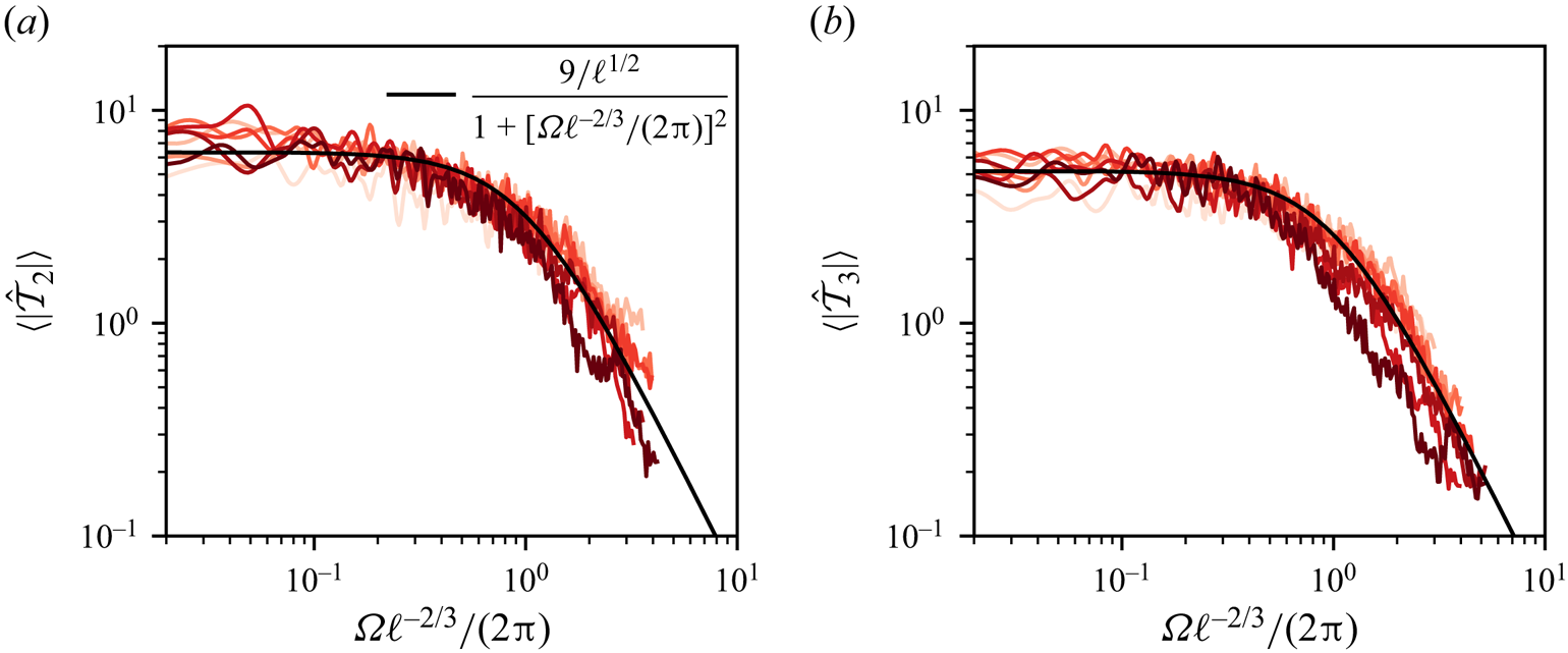
To characterize the temporal evolution of the effective forcing $\mathcal {T}_\ell$, we study its ensemble-averaged Fourier transform $\langle |\hat {\mathcal {T}}_\ell | \rangle$. Injecting (3.4) and (3.10) within (3.5) we obtain an expression in Fourier space for $\langle |\hat {\mathcal {T}}_\ell | \rangle$

(3.18)\begin{equation} \langle |\hat{\mathcal{T}}_\ell| \rangle(\varOmega) = \langle |\hat{x}_\ell| \rangle(\varOmega) \cdot \left [{(\varOmega^2 - \varOmega_\ell(\textit{We})^2)^2 + \varLambda_\ell^2 \varOmega^2} \right]^{1/2}. \end{equation}

Figures 7(a) and 7(b) show $\langle |\hat {\mathcal {T}}_2| \rangle$ and $\langle |\hat {\mathcal {T}}_3| \rangle$, respectively, as a function of $\varOmega \ell ^{-2/3}$, where $\ell ^{2/3}$ is the eddy turnover time at scale $d/\ell$ (in units of $t_c(d)$). For all frequencies, we found that the effective forcing spectrum does not depend on the Weber number. At low frequencies ($\varOmega <1.3 \, \ell ^{2/3}$), the forcing amplitude is constant, corresponding to a white noise. For $\varOmega >2 {\rm \pi}\ell ^{2/3}$, the decay of $\langle |\hat {\mathcal {T}}_\ell | \rangle$ is compatible with $1/\varOmega ^2$. The limit between these two regimes is set by the eddy turnover time at scale $d/\ell$. We found that the spectrum of the effective forcing only depends on the turbulence parameters, and is therefore independent of the bubble deformations. As was anticipated in § 3.1, model (3.1) decouples the turbulent forcing (the right-hand side) from the bubble response (the left-hand side). The observation of a cutoff frequency at the characteristic time scale of turbulent fluctuations at the mode scale $d/\ell$ can be interpreted as a filtering process originating from the integration over the bubble surface. This filtering operation is further discussed in § 5.

Figure 7.

Effective forcing spectrum for $\ell =2$ (a) and $\ell = 3$ (b) deduced from (3.18) as a function of the frequency normalized by the eddy turnover time at scale $d/\ell$. The Weber number is colour coded with the same colour bar as in figure 2.

From the previous observations, we propose the following expression for the forcing spectrum:

(3.19)\begin{equation} \langle |\hat{\mathcal{T}}_\ell| \rangle(\varOmega) = \frac{\tau_\ell}{ 1 + [\varOmega \ell^{-2/3}/(2{\rm \pi})]^2}, \end{equation}

where $\tau _\ell$ is a numerical constant, accounting for the $\ell$-dependency of $\mathcal {T}_\ell$, that is adjusted on the data. From (3.6) and figure 3, we estimate $\tau _\ell \sim \ell ^{-1/2}$. The expression (3.19) captures quantitatively the effective forcing spectrum (solid black line in figure 7(a,b).

In the context of Lagrangian particle accelerations, Voth et al. (Reference Voth, La Porta, Crawford, Alexander and Bodenschatz2002), followed by Volk et al. (Reference Volk, Calzavarini, Verhille, Lohse, Mordant, Pinton and Toschi2008), computed the temporal autocorrelation of inertial particle accelerations in turbulence. The temporal acceleration statistics of a finite-size particle is usually attributed to a filtering effect of the small-scale turbulent fluctuations at the particle scale (Qureshi et al. Reference Qureshi, Bourgoin, Baudet, Cartellier and Gagne2007). As a consequence, the correlation time of acceleration for a neutrally buoyant particle is given by the eddy turnover time $t_c(d)$. This result has been recently extended to a buoyant particle that exhibits a modified correlation time $t \sim t_c(d) \beta ^{-1/2}$ (Fan et al. Reference Fan, Wang, Jiang, Sun and Calzavarini2024), where $\beta = 3 \rho /(2 \rho + \rho _p)$ is a function of the fluid density $\rho$ and the particle density $\rho _p$. For a bubble, we have $\beta = 3$, corresponding to a correlation time of order $t_c$. In our case, the temporal auto-correlation function $C_{\mathcal {T}_\ell }(t) = \langle \mathcal {T}_\ell (0) \mathcal {T}_\ell (t)\rangle / (\sigma _\mathcal {T}^\ell )^2$ for the modes $\ell >1$ can be deduced from the spectrum $\hat {\mathcal {T}}_\ell$ and is written as

(3.20)\begin{equation} C_{\mathcal{T}_\ell}(t) = \exp(-2{\rm \pi} \ell^{2/3}t)(1 + 2{\rm \pi} \ell^{2/3}t). \end{equation}

We found that the correlation time in physical units is given by $t_c(d) \ell ^{-2/3}/(2 {\rm \pi})$, which also scales as $t_c(d)$, with an additional dependency on the mode order $\ell$. The prefactor being smaller than one, the mode oscillations decorrelate faster that the velocity fluctuations at the bubble scale.

In summary, we found that all the statistics of $\mathcal {T}_\ell$ are independent of $\textit {We}$, which confirms the initial intuition of Risso & Fabre (Reference Risso and Fabre1998) that the bubble dynamics and turbulent forcing are decoupled. We found that the bubble deformation by the flow field can be described by a one-way coupling model: the flow field generated by bubble oscillations does not significantly impinge back on the bubble dynamics. In addition, experimental results from the literature suggest that these statistics are likely to be independent of $\textit {Re}(d)$, as long as we consider bubbles larger than the Kolmogorov scale.

From the stationary hypothesis (H3), the forcing is completely characterized by its distribution and temporal autocorrelation function. The combination of an explicit form for the p.d.f. (3.16) and for the autocorrelation function (3.20) then provides a complete model of a synthetic stochastic effective forcing for bubble deformations in turbulence. Previous modelling approaches have used two-point velocity measurements to model an effective forcing term (Risso & Fabre Reference Risso and Fabre1998; Lalanne et al. Reference Lalanne, Masbernat and Risso2019; Masuk et al. Reference Masuk, Salibindla and Ni2021b), following the original idea from Kolmogorov (Reference Kolmogorov1949) and Hinze (Reference Hinze1955). Here, we found that the statistics of the effective forcing differ significantly from two-point statistics, in particular due to the volumetric filtering effect at the particle size.

4.1. Modes’ standard deviation and distributions

We first look at the modes’ standard deviation $\sigma _x^\ell$.

Figure 8(a) shows the modes’ standard deviation of the DNS as a function of the Weber number for $\ell \in [2, 5]$. We find that $\sigma _x^\ell$ can be approximated by $\sigma _x^\ell \approx \textit {We}/[(\ell -1)(\ell +1)(\ell +2)]$, with a constant of order one. We compute $\sigma _x^\ell$ from the model in Fourier space using expressions of (3.4), (3.10) and (3.19) and the Parseval identity. The results are superimposed by the solid line for $\ell = 2$ and 3, showing a quantitative agreement with the numerical data.

Figure 8.

(a) Modes’ standard deviation as a function of the Weber number for all $\ell$. The two solid lines are the results from our linear model, for modes $\ell =2$ and $\ell =3$. (b) Modes’ standard deviation compensated by $We$ as a function of the mode principal number.

A scaling for $\sigma _x^\ell$ as a function of $\textit {We}$ and $\ell$ can be deduced analytically in model cases. One natural case is to consider $\mathcal {T}_\ell$ as a Gaussian white noise of autocorrelation function $C(t) = D \delta (t)$, where $\delta$ is the Dirac function, and $D$ is independent of the Weber number. In this case, from the analysis of stochastic harmonic oscillators (Gitterman Reference Gitterman2005), the standard deviation reads

(4.1)\begin{equation} \sigma_x^\ell \sim \left [ \frac{D}{\varLambda_\ell \varOmega_\ell^2}\right ]^{1/2}. \end{equation}

From the coefficients $\varLambda _\ell$ and $\varOmega _\ell$ we extracted, this model predicts $\sigma _x^\ell \propto \textit {We}^{1/2}$, which does not correspond to the observed scaling. A finite correlation time has been taken into account. We then consider $\mathcal {T}_\ell$ as an exponentially correlated Gaussian noise of autocorrelation function $\langle \mathcal {T}_\ell (t) \mathcal {T}_\ell (t^\prime )\rangle = (\sigma _\mathcal {T}^\ell )^2 \exp ( - |t - t^\prime |/t_\ell )$, where $t_\ell = \ell ^{-2/3}/(2 {\rm \pi})$ is the correlation time of the effective forcing deduced from (3.20), and $D$ is independent of $\textit {We}$. In this case, the mode's standard deviation reads (Gitterman Reference Gitterman2005)

(4.2)\begin{equation} \sigma_x^\ell = \sigma_\mathcal{T}^\ell \left[\frac{ t_\ell (1 + \varLambda_\ell t_\ell)}{ \varOmega_\ell^2 \varLambda_\ell( 1 + \varLambda_\ell t_\ell + \varOmega_\ell^2 t_\ell^2)} \right ]^{1/2}. \end{equation}

The scaling of $\sigma _x^\ell$ now becomes a function of the ratios $\varLambda _\ell t_\ell$ and $\varOmega _\ell t_\ell$. In practice, we have $\varOmega _\ell t_\ell \gg 1$ and $\varOmega _\ell t_\ell \gg \varLambda _\ell t_\ell$ for sufficiently small Weber. Considering the limit $\varLambda _\ell t_\ell \gg 1$, (4.2) simplifies as

(4.3)\begin{equation} \sigma_x^\ell =\frac{\sigma_\mathcal{T}^\ell}{\varOmega_\ell^2} = \frac{\sigma_\mathcal{T}^\ell}{(\ell -1)(\ell + 1)(\ell +2)}\textit{We}. \end{equation}

We then recover the observed scaling for small Weber number. For larger Weber number, the ratio $\varOmega _\ell t_\ell$ decreases, and we expect a transition to a shallower increase of $\sigma _x^\ell$ with $We$. This transition should occur for larger Weber number as $\ell$ increases, an interpretation compatible with the numerical data shown in figure 8(a). The observed scaling of $\sigma _x^\ell$ with Weber number thus corresponds to a saturation of the bubble deformations dominated rather by the long correlation time of the forcing (frozen turbulence hypothesis applied to bubble deformations Ruth et al. Reference Ruth, Mostert, Perrard and Deike2019) than an accumulation of random forcing events on a time scale $1/\varLambda _\ell$. It is worth noticing that the estimate of the correlation time of the forcing is therefore essential to predict the amplitude of bubble deformations.

To further check the dependency on $\ell$, figure 8(b) shows the compensated standard deviation $\sigma _x^\ell /\textit {We}$. We recover that the decrease of the modes’ amplitude with $\ell$ can be mainly attributed to the increase of the natural frequency with $\ell$, with a small correction originating from the weak dependency of $\mathcal {T}_\ell$ with $\ell$. Eventually, we found a quantitative agreement between the standard deviation $x_\ell$ and the result from the linear model. The model captures the evolution of $\sigma _x^\ell$ with both $We$ and $\ell$.

The linear increase of $\sigma _x^\ell$ with $We$, up to $\textit {We} \approx 3$, has important consequences when modelling bubble breakup. Risso & Fabre (Reference Risso and Fabre1998) suggested that the threshold for breakup is close to the value above which the deformations start to be nonlinear. A linear model would then be sufficient to describe bubble deformations up to the breakup threshold.

We then look at the entire statistics of $x_\ell$. Figure 9 shows the probability density functions of the modes $\ell =2$ for all Weber numbers (9a) normalized by their standard deviation. We find that the shape of the p.d.f. does not depend on the Weber number and corresponds to the hyperbolic secant distribution (black dashed line), equivalent to the p.d.f. of the effective force $\mathcal {T}_\ell$. Both the forcing and the mode amplitude share the same p.d.f. that deviates from Gaussianity (solid black line) with exponential tails. As the distributions exhibit fat tails, the probability that bubbles experience large deformations leading to breakup is large compared with a Gaussian distribution (black dotted line). Moreover, for larger $\ell$, the deviation from a Gaussian distribution increases, as shown in figure 9(b) for $\textit {We}=1$.

Figure 9.

(a) Normalized p.d.f. of $x_2$ for all $We$. (b) Normalized p.d.f. at $\textit {We}=1$ for different $\ell$. In both panels the black dashed line is the hyperbolic secant distribution. The solid black line the Gaussian distribution.

4.2. Deformation spectrum

Figure 10 compares the modes’ Fourier transforms with the model (3.5) combined with (3.10), (3.4) and (3.19) (dotted lines). For all Weber numbers, the model accurately reproduces the zero-limit frequency as well as the amplitude of the spectrum at the bubble natural frequency $f_2$ and the position and slope of the decay at larger frequencies. At the lowest Weber number ($\textit {We} = 0.27$), the model overestimates the spectrum just below the resonance. We remind the reader here that, for angular frequencies larger than $3\varOmega _2$, the spectrum is dominated by numerical noise. For all other $We$, in the absence of resonance, the model captures the spectrum close to the bubble natural frequency.

Figure 10.

Comparison of the Fourier spectrum amplitude between the DNS and the model (dotted line). The model spectrum is obtained by combining (3.10), (3.4) and (3.19) in (3.5), for the mode $\ell =2$. The model captures the low-frequency limit, the position of the transition as well as the high-frequency decay for all $We$.

4.3. Consequences for bubble breakup

Thanks to the quantitative model we have developed, we can revisit the breakup scenario and the criterion for breakup. Two main breakup scenarios have been proposed for bubbles in turbulence. Bubbles can break either when they encounter a turbulent fluctuation larger than some threshold value (Lee et al. Reference Lee, Erickson and Glasgow1987; Luo & Svendsen Reference Luo and Svendsen1996; Wang et al. Reference Wang, Wang and Jin2003; Masuk et al. Reference Masuk, Qi, Salibindla and Ni2021a) or after a series of small excitations at their natural frequency which induce a resonance (Sevik & Park Reference Sevik and Park1973; Risso & Fabre Reference Risso and Fabre1998). The ability of a bubble to store energy in a mode $\ell$, is quantified by the quality factor $Q_\ell = \varOmega _\ell /\varLambda _\ell$. The quality factor $Q_\ell$ sets the number of periods over which energy can be stored. For large $Q_\ell$, energy can be accumulated, while it is dissipated in a few bubble periods for low $Q_\ell$. Our linear model provides a quantitative measure of $Q_\ell$. Combining (3.4) and (3.10) we have an explicit expression for $Q_\ell$ as a function of $We$ and $\ell$

(4.4)\begin{equation} Q_\ell = 4\sqrt{\frac{(\ell - 1)(\ell +1)}{0.6(\ell +2)(2\ell +1)^2}}\textit{We}^{-1/2}. \end{equation}

In turbulence, bubbles mainly break after oblate–prolate deformations, meaning deformations along their second modes $\ell =2$ (Risso & Fabre Reference Risso and Fabre1998; Ravelet et al. Reference Ravelet, Colin and Risso2011; Masuk et al. Reference Masuk, Salibindla and Ni2021b; Perrard et al. Reference Perrard, Rivière, Mostert and Deike2021). For the typical critical Weber numbers reported in the literature, $0.1 <\textit {We}_c <10$ (Sevik & Park Reference Sevik and Park1973; Risso & Fabre Reference Risso and Fabre1998; Martínez-Bazán, Montanes & Lasheras Reference Martínez-Bazán, Montanes and Lasheras1999; Rivière et al. Reference Rivière, Mostert, Perrard and Deike2021), our estimate of the quality factor for the mode $\ell =2$ ranges from $0.3$ ($\textit {We}_c = 10$) to 3 ($\textit {We}_c = 0.1$). These quality factors are too small to observe significant energy storage over several periods of oscillations. Resonance can still occur for the largest $Q_\ell \approx 3$. However, we expect the resonant mechanism to be subdominant at this quality factor. We conclude that bubbles break from short and large turbulent fluctuations rather from a series of small excitations at the bubble natural frequency (resonant mechanism).

Note that a sequence of oscillations at the bubble natural frequency may be observed for sufficiently large quality factor, typically $Q_2>10$, corresponding to $\textit {We}<8\times 10^{-3}$. Even though such a Weber number corresponds to a bubble size much smaller than the Kolmogorov Hinze scale, which will never break, a resonant breakup may be observed experimentally.

5.1. Point statistics of the pressure field

As a reference case, we first consider the Eulerian point statistics of pressure in homogeneous and isotropic turbulence, at the same Taylor Reynolds number $\textit {Re}_\lambda = 55$, corresponding to the two-phase flow case. To compare with the bubble dynamics, we will still express length scales in units of $d$, time scales in units of $t_c(d)$ and therefore velocity in terms of velocity increments at the bubble scale $\langle \delta u(d)^2 \rangle ^{1/2}$.

We run single-phase DNSs and record the Eulerian pressure fluctuations $p(x, t)$ at seven different fixed locations well separated in space. We run three simulations for a total of $245 t_c(d)$. Resolution is increased compared with the two-phase problem and would be equivalent to 68 points per bubble radius and 3.6 points per Kolmogorov length. Note that increasing the resolution was not necessary but allows us to obtain more precise results, especially in the viscous range. In this section, ensemble averages are performed over the three simulations and the seven locations.

Figure 11(a) illustrates two temporal evolutions of pressure, normalized by the characteristic pressure difference at the bubble scale, $P_c= \rho \delta u(d)^2$. We found a pressure standard deviation $\sigma _p = 0.67 P_c$. Pressure exhibits random oscillations of small amplitude around zero, together with large negative drops. This asymmetry between positive and negative fluctuations is better observed on the pressure p.d.f. plotted in figure 11(b). We recover that negative values are exponentially distributed, while positive values follow a Gaussian distribution (dashed black line). The existence of the large negative peaks leading to an asymmetric p.d.f. is well known and has been reported both in experiments (Abry et al. Reference Abry, Fauve, Flandrin and Laroche1994; Pumir Reference Pumir1994; Cadot, Douady & Couder Reference Cadot, Douady and Couder1995) and DNSs of homogeneous isotropic turbulence (Cao, Chen & Doolen Reference Cao, Chen and Doolen1999; Vedula & Yeung Reference Vedula and Yeung1999). It has been shown that these large negative peaks correspond to vorticity filaments (Douady, Couder & Brachet Reference Douady, Couder and Brachet1991; Fauve, Laroche & Castaing Reference Fauve, Laroche and Castaing1993; Cadot et al. Reference Cadot, Douady and Couder1995) passing through the measurement point. As the bubble moves in the fluid, it may experience different pressure statistics and the Lagrangian pressure statistics could also be relevant.

Figure 11.

(a) Typical temporal evolution of the pressure at two points in space. We observe small-amplitude oscillations together with rare intense negative peaks. (b) Local pressure distribution normalized by its standard deviation $\sigma _p = 0.67 P_c$. The solid black line follows the hyperbolic secant distribution centred while the black dashed line follows a Gaussian distribution with standard deviation $4/5$.

Lagrangian pressure statistics have also been investigated numerically. Numerical studies involve measuring pressure statistics along the paths of point particles (Bappy, Carrica & Buscaglia Reference Bappy, Carrica and Buscaglia2019), as well as (sub-Kolmogorov) finite-size bubbles (Bappy et al. Reference Bappy, Carrica, Vela-Martín, Freire and Buscaglia2020a,Reference Bappy, Vela-Martin, Buscaglia, Carrica and Freireb) whose dynamics is modelled using a pure advection or a Maxey–Riley equation (Maxey & Riley Reference Maxey and Riley1983; Toschi & Bodenschatz Reference Toschi and Bodenschatz2009), respectively. They found that larger particles have a higher probability of being within low pressure regions. Nevertheless, the overall shape of the pressure p.d.f., with an exponential tail for negative values and a Gaussian distribution of positive values, is conserved.

To investigate the frequency statistics of the local pressure, we compute the temporal Fourier transform of each pressure signal $\hat {p}$

(5.1)\begin{equation} \hat{p}(\varOmega) = \frac{1}{T}\int_{0}^T p(t) {\rm e}^{-{\rm i} \varOmega t} \,{\rm d}t. \end{equation}

The average amplitude of its Fourier transform $\langle |\hat {p}| \rangle$ is plotted in figure 12. The corresponding inertial range in frequency space is delimited by the inverse of the eddy turnover time at the integral scale $\varOmega _c(L) = 2 {\rm \pi}/t_c(L)$ (black dotted line) and the inverse of the eddy turnover time at the Kolmogorov scale, $\varOmega _c(\eta )$ (dashed line). For low frequencies, $\varOmega <\varOmega _c(L)$, $\langle |\hat p| \rangle$ slowly decreases with $\varOmega$. Abry et al. (Reference Abry, Fauve, Flandrin and Laroche1994) have shown that this evolution at low frequencies originates from the contribution of vorticity filaments, since their typical lifetime is the integral time scale (Douady et al. Reference Douady, Couder and Brachet1991; Pumir Reference Pumir1994). Removing their contributions flattens the low-frequency spectrum (Abry et al. Reference Abry, Fauve, Flandrin and Laroche1994).

Figure 12.

(a) Amplitude of the local pressure Fourier transform. The vertical dotted line corresponds to the angular frequency $\varOmega _c(L)$ of eddies of integral length scale in size, while the dashed line corresponds to the angular frequency $\varOmega _c(\eta )$ of eddies of Kolmogorov length scale in size. Inset plot: compensated Fourier transform $\langle |\hat {p} | \rangle / \hat {p}^{K}$. The solid line corresponds to $\langle |\hat {p}| \rangle = \hat {p}^{K}/10$.

In the inertial range of the turbulent cascade, $\varOmega _c(L)<\varOmega <\varOmega _c(\eta )$, $\langle |\hat {p}|\rangle$ decays down to the noise level near $\varOmega _c(\eta )$. In the spatial Fourier space, and a fortiori in the temporal Fourier space, there is no consensus for the scaling of the pressure power spectrum within the inertial range (Pullin & Rogallo Reference Pullin and Rogallo1994). A Kolmogorov-like scaling predicts $|\hat {p}(k)|^2 \sim \epsilon ^{4/3} k^{-7/3}$ with k the mode's wave number (reported by Ishihara et al. (Reference Ishihara, Kaneda, Yokokawa, Itakura and Uno2003) for instance) but other authors have also reported a $k^{-5/3}$ scaling (Gotoh & Rogallo Reference Gotoh and Rogallo1999; Vedula & Yeung Reference Vedula and Yeung1999). To transform the spatial power spectrum into a temporal power spectrum, a classical way is to consider that the small-scale structures are advected by the large scales. This is the sweeping hypothesis (Kraichnan Reference Kraichnan1964; Tennekes Reference Tennekes1975), which has been successfully used to reproduce pressure temporal autocorrelation (Yao et al. Reference Yao, He, Wang and Zhang2008). Combining this argument with the Kolmogorov prediction, we find that $\langle \hat {p} \rangle$ should scale as $\hat {p}^K \sim \epsilon ^{2/3} u_{rms}^{5/6} \varOmega ^{-4/3}$, with a proportionality constant of order 1. We find a reasonable agreement, as shown by the compensated spectrum $\langle \hat {p} \rangle /\hat {p}^K$ in the inset of figure 12. As evidenced by Pumir (Reference Pumir1994), Pullin & Rogallo (Reference Pullin and Rogallo1994) and Vedula & Yeung (Reference Vedula and Yeung1999), the Kolmogorov scaling might only hold in a narrow range of frequencies, corresponding to scales just below the integral scale, due to the limited inertial range. The proportionality constant is around 0.1 in our case (solid black line) lower than the value of 7 proposed by Pumir (Reference Pumir1994). The third regime $\varOmega >\varOmega _c(\eta )$, corresponds to the end of the inertial range and is close to the limit of resolution of our DNS, as $\varOmega _c({\Delta x}) = 3 \varOmega _c(\eta )$, where $\Delta x$ is the minimum grid size.

5.2. Pressure field on a sphere

To compare the pressure statistics with the effective forcing $\mathcal {T}_\ell$, we interpolate the pressure field $p_S(\theta,\phi )$ in the single-phase DNS on a sphere of radius $R_0$, and compute its spherical harmonic decomposition

(5.2)\begin{equation} p_S(\theta, \phi) = P_c \left[\sum_{\ell = 0}^\infty \sum_{m =-\ell}^\ell P_{\ell, m}(t)\,Y_\ell^m(\theta, \phi)\right]. \end{equation}

Similarly to the modes of deformation $x_{\ell, m}$, the statistics of $P_{\ell, m}$ are independent of $m$. Ensemble averages are then computed over the three simulations and the $m$ values. For pressure, the modes $\ell =0$ and $\ell = 1$ are non-zero, however, we focus in the following on modes $\ell \geq 2$, which are relevant for bubble deformations. Figure 13(a) shows that the standard deviation of each mode $\ell$, $\sigma _P^\ell$, varies exponentially with $\ell$. A higher $\ell$ is associated with fluctuations at a smaller scale, which are known to be less energetic. However, we have no explanation for the exponential scaling. We also observed a decay of $\sigma _\mathcal {T}^\ell$ with $\ell$ (figure 5). The symmetry between positive and negative values is restored, as shown in figure 13(b). Distributions now show exponential tails for both negative and positive pressure values. The shape of the distribution is found to be independent of $\ell$, corresponding to the same hyperbolic secant distribution (3.16) as the effective forcing distribution we previously identified.

Figure 13.

(a) Pressure standard deviation, $\sigma _P^\ell$ as a function of $\ell$, showing an exponential decay with $\ell$ (black dotted line). (b) Distributions of $P_\ell$, normalized by $\sigma _P^\ell$, as a function of $\ell$. All the pressure modes share the forcing distribution given in (3.16).

Eventually, we compute the temporal Fourier transform $\hat {P}_\ell$ of the spherical pressure modes $P_\ell$. Figure 14(a) shows the ensemble average of the norm, $\langle |\hat {P}_\ell | \rangle$ as a function of the frequency. For each $\ell$, we recover the three regimes we observed for the point pressure spectrum and $\mathcal {T}_\ell$. The transition between the two first regimes depends on the mode $\ell$. Considering that the pressure spectrum shares the same characteristic frequency as the effective forcing spectrum, we expect the transition to occur at $\varOmega = 2 {\rm \pi}\ell ^{2/3}$, the frequency associated with eddies of size $d/\ell$, in units of $t_c(d)$. We show in figure 14(b) the spectra $\langle |\hat {P}_\ell | \rangle$ normalized by their low-frequency limit, $\hat {P}_\ell ^0$, as a function of the frequency normalized by $\ell ^{2/3}$, the eddy turnover time at scale $d/\ell$. All curves collapse onto a single master curve, showing that the pressure and effective forcing share the same time scales. Below the critical frequency ($\varOmega <\varOmega _\ell$), the spectrum amplitude converges to a constant value, significantly above the integral frequency $\varOmega _L$. Similarly to Abry et al. (Reference Abry, Fauve, Flandrin and Laroche1994), the pressure spectrum at low frequency is now constant. We can assume that the averaging over the sphere has filtered the contribution from localized structures, and in particular the vorticity filaments. A flat spectrum in the range $\varOmega _c(L)<\varOmega <2 {\rm \pi}\ell ^{2/3}$ also indicates that the contribution of eddies larger than $d/\ell$, which are roughly homogeneous at the mode scale, has also been filtered out: a bubble is mainly deformed by eddies at its scale. For $2 {\rm \pi}\ell ^{2/3}<\varOmega <\varOmega _\eta$, $\langle |\hat {P}_\ell | \rangle$ follows $\varOmega ^{-3}$. This decay is steeper than the $\ell$-dependency of $\langle |\hat {\mathcal {T}}_\ell | \rangle$ which follows $\varOmega ^{-2}$. This might be attributed to the discrepancy between Eulerian and Lagrangian statistics. From the sweeping effect (Kraichnan Reference Kraichnan1964), the temporal decorrelation of Eulerian quantities is expected to occur faster than their Lagrangian counterpart.

Figure 14.

(a) Amplitude of the pressure Fourier transform $\langle |\hat {P}_\ell | \rangle$ for each mode $\ell$ as a function of the angular frequency in units of the eddy turnover time at the bubble scale. The black dashed line represents the eddy turnover time at scale $\eta$. The black dotted line is the eddy turnover time at the integral length scale. (b) Normalized pressure Fourier transform as a function of frequency in units of the eddy turnover time at scale $d/\ell$. The black line follows $\varOmega ^{-3}$.

To summarize, we have shown that the effective forcing $\mathcal {T}_\ell$ deforming a bubble shares the same statistics as the corresponding pressure mode on a sphere of the same radius. As a consequence of the filtering effect induced by the integration over a sphere, the characteristic frequency associated with each mode $\ell$ is the eddy turnover time at scale $d/\ell$, the frequencies smaller than $\ell ^{2/3}$ are well described by a white noise and the forcing amplitude decreases with $\ell$.

5.3. Dissipation profiles

Our analysis of bubble deformation shows that (i) the effective forcing originates from turbulent fluctuations near the bubble, and it is not affected by bubble deformability. (ii) The damping of bubble oscillations is significantly enhanced compared with the quiescent case. This damping can either originate from additional dissipation in the turbulent boundary layer or an energy transfer from the bubble oscillations to the turbulent flow. Both mechanisms depend on the boundary layer thickness. Using a turbulent viscosity hypothesis we estimated that energy was transported on a boundary layer of size $L_t = R_0 /5$, independent of $We$. In this section we investigate the velocity gradient profile near the bubble, on a distance comparable to bubble typical deformation. To do so, we need to compute a local distance $r$ to the interface, which is not provided by the Basilisk volume of fluid (VOF) algorithm.

The method principle is the following. For every bulk point, we find the closest grid point on the interface. We then interpolate the bubble surface around this point, using a quadratic interpolation on the $20$ closest neighbouring interfacial points. To find the neighbours efficiently, the interfacial grid points are stored in a $k-d$ tree structure. The distance $r$ to the interface is then found by minimizing the distance from the bulk point to the quadratic manifold. We follow this procedure for both outside ($r>0$) and inside ($r<0$) bulk points.

We diagnose the additional dissipative term of the linear model by investigating the local dissipation rate profile around the bubble. The energy dissipation rate per unit of mass in a elementary volume is related to the local velocity gradients by

(5.3)\begin{equation} \langle \epsilon \rangle(x) = 2 \nu \langle (\partial_i u_j + \partial_j u_i)^2 \rangle, \end{equation}

where we use Einstein notations. For each run, we output snapshots of the full flow field at times separated by at least one eddy turnover time at the bubble scale, to ensure statistical independence. We then compute profiles of the local dissipation near the interface by averaging on shells of constant distance from the bubble interface, as illustrated in figure 15. Eventually, for each Weber number, we ensemble average the flow snapshots (see table 3) to extract a mean profile.

Figure 15.

Example of the distance computation on a slice of a bubble at $\textit {We} = 2$. The red points are on the interface. Isocontours are separated by $0.0625R_0$. We also show the association between one bulk points and the corresponding interfacial point.

Table 3.

Number of snapshots per Weber number used to compute the flow profiles.

Figure 16(a) shows the average local dissipation, divided by the kinematic viscosity, $\langle \epsilon \rangle (r)/\nu$, as a function of the distance $r$ to the bubble interface. Far from the bubble interface, for $r>R_0/2$ and $r<-R_0/2$, the local dissipation converges to a constant. In the gas, velocity gradients are maximum at $r=-R_0/15$. The existence of a maximum inside the bubble near the interface originates from the nearly no-slip boundary condition imposed by the denser fluid on the gas inside the bubble. A similar boundary layer has indeed been observed near a solid particle's surface (no-slip boundary condition) (Shen et al. Reference Shen, Peng, Wu, Chong, Lu and Wang2022; Chiarini & Rosti Reference Chiarini and Rosti2024). For bubbles, we therefore expect that decreasing the gas density increases the amplitude of the peak. The velocity gradients inside and outside the bubble share the same order of magnitude: the dissipation hence mainly takes place outside the bubble, in the liquid, where the dynamical viscosity is much larger. To understand the origin of the additional damping we then focus on the outside boundary layer.

Figure 16.

(a) Local velocity gradient inside and outside the bubble as a function of the distance to the interface, for all $We$. (b) Limit of the dissipation rate at the bubble interface in the liquid phase as a function of the Weber number.

For $r>0$, we observe a thick boundary layer of typical size $R_0/5$ (see figure 16a), compatible with our estimation of $L_t$ (see (3.13)). Figure 16(b) shows the dissipation rate value at the interface in the liquid $\langle \epsilon \rangle |_{0^+}$ as a function of the Weber number. At vanishing Weber number, we find a non-zero dissipation originating from a geometrical boundary layer. The interfacial value varies between 3 times ($\textit {We} = 0.27$) and four times ($\textit {We} = 2$) larger than that in the bulk. In addition, we find an increase compatible with a linear dependency of the interfacial dissipation with $We$. If we interpret this additional dissipation as an energy transfer rate from the surface deformation to the flow, it would scale as $\varLambda _\ell (\dot {x}_\ell )^2$. We have $(\dot x_\ell )^2 \sim (\omega ^q_\ell \sigma _x^{\ell })^2 \propto \textit {We}$. This interpretation is therefore compatible with a damping coefficient $\varLambda$ independent of $\textit {We}$.

In the absence of flow, the thickness of the boundary layer of the oscillating bubble can be estimated by $\sqrt {2\nu /\omega _2^q}$. For a Weber number ranging from 2.9 to 0.27, this estimation gives a boundary layer of size ranging from $0.07R_0$ to $0.04R_0$, which is much thinner than the boundary layer thickness we measured. We conclude that the boundary layer is geometric. It is not produced by bubble oscillations. The existence of a thick boundary layer was completely disregarded in the computation of Lamb (Reference Lamb1932) for a potential flow far from the interface. The thick boundary layer we observed for the dissipation profile is then consistent with an effective damping one order of magnitude larger than in the quiescent case.