NOMENCLATURE
- C(u)
class function
- S(u)
shape function
- u
chord length position
-
 $A_R$
class shape transformation coefficients
- n
Bernstein polynomial power
-
$z_o/z_p$
original/perturbed z coordinate
-
$N_{cr}$
critical N-factor
-
$N_i$
ideal critical N-factor
-
$N_\sigma$
standard deviation of critical N-factor
- F
output variable function
-
$P(N_{cr})$
probability density function
- W
summation of weights
-
$k_r$
number of
$N_{cr}$
samples-
$Tr_u$
upper-surface transition location
-
$Tr_l$
lower-surface transition location


Greek symbol
-
$\Delta_{z_{te}}$
trailing-edge thickness
-
$\mu$
mean
-
$\sigma$
standard deviation


1.0 INTRODUCTION
The passive extension of laminar flow over an aerodynamic surface, referred to as Natural Laminar Flow (NLF), is seen as a promising approach for the reduction of aircraft drag(Reference Thomas1). Obtaining NLF requires the suppression of boundary-layer instabilities, which are the cause of flow transition. This is achieved during NLF aerofoil design by tailoring the aerofoil’s pressure distribution. However, the sensitivity of the transition location to the surface and flow quality makes effective implementation of NLF challenging. Early transition of the flow can occur for a number of reasons. These include contamination of the leading edge by insects, icing or debris(Reference Wagner and Fischer2,Reference van Dam and Holmes3) , as well as in the presence of steps and gaps between panels or other irregularities in the surface finish and roughness(Reference Braslow and Fischer4,Reference Joslin5) .
Manufacturing aerodynamic surfaces without steps, gaps and other irregularities is difficult and costly. Methods for protecting the wing from contamination have also been proposed(Reference Young and Humphreys6). However, these are often complex and not able to guarantee contamination is avoided. An alternative to this is to obtain a NLF design that is insensitive to variations in the surface and flow quality. This is achieved using the robust design approach pioneered by Genichi Taguchi(Reference Taguchi and Wu7) that tries to improve the mean performance while reducing the standard deviation of the performance in the presence of uncertainty. To some degree, it can be considered an extension of multi-point design, which tries to improve the net performance at a range of conditions and has also been applied to the design of NLF aerofoils(Reference Robitaille, Mosahebi and Laurendeau8,Reference Rashad and Zingg9) .
There has been extensive research on the robustness of fully turbulent aerofoils to uncertainty in the Mach and Reynolds numbers(Reference Huyse and Lewis10–Reference Cook, Jarrett and Willcox19), but less applied to NLF design. Zhao et al.(Reference Zhao, Dawes, Parks, Jarrett and Yang20) carried out shape optimisation of a NLF aerofoil to improve the robustness of the maximum lift coefficient (
 $C_{l,{\rm max}}$
) to uncertainty in the transition location. Zhao et al.(Reference Zhao, Gao and Huang21) then carried out shape optimisation of a NLF aerofoil to improve the robustness of the drag to uncertainty in the Mach number. Jing et al.(Reference Jing, Zhenghong, Jiangtao and Ke22) also performed shape optimisation of an NLF aerofoil to improve the robustness of the drag to uncertainty in the Mach number and lift coefficient. While these studies consider the robustness of NLF performance to uncertainty in flight conditions or the transition location itself, research on the robustness of NLF aerofoils to uncertainty in the surface and flow quality has been limited. Salahudeen and Baeder(Reference Salahudeen and Baeder23) analysed the sensitivity of an aerofoil with a free transition to uncertainty in the flow quality by varying the free-stream turbulent intensity in the transport equation-based
 $\gamma-\text{Re}_\theta$
transition model.
Modelling instability growth within the boundary layer is done using linear stability theory. The
 $e^N$
transition model makes use of this by prescribing the transition at the point at which an instability wave first exceeds some critical amplification factor. This is typically referred to as the critical N-factor (
 $N_{cr}$
). The transition occurs at a lower
 $N_{cr}$
value, and so further upstream, if the surface or flow quality is reduced. It is therefore possible to approximate the effects of uncertainty in the surface and flow quality by applying uncertainty to the value of
 $N_{cr}$
within the
 $e^N$
transition model. Some work has been done using this relationship. Deng and Qiao(Reference Deng and Qiao24) used an inverse design approach to obtain a NLF aerofoil with an
 $N_{cr}$
envelope that sees little change in the transition location as
 $N_{cr}$
is reduced. Han et al.(Reference Han, Chen, Zhu and Song25) optimised a NLF wing using
 $N_{cr}$
values lower than expected to account for the uncertainty in real flight conditions. Rashad and Zingg(Reference Rashad and Zingg9) analysed this approach and found that optimising for a reduced
 $N_{cr}$
was no guarantee of performance at higher
 $N_{cr}$
, given that extended laminar flow can increase the risk of flow separation. They then carried out multi-point optimisation over three
 $N_{cr}$
values to ensure that aerofoil performance was maintained at off-design conditions.
There are two main objectives to this study. The first is to investigate the sensitivity of aerofoil performance to uncertainty in
 $N_{cr}$
. The second objective is to carry out robust shape optimisation with the goal of improving the robustness of aerofoils to uncertainty in
 $N_{cr}$
. In both cases, uncertainty in
 $N_{cr}$
is used to qualitatively account for the uncertainty in the surface and flow variability. While direct modelling of surface and flow quality effects on the transition lies beyond the scope of this study, it is assumed that these unknowns may be crudely incorporated through a reduced
 $N_{cr}$
criterion.
2.0 ANALYSIS METHODOLOGY
2.1 Uncertainty distribution
The uncertainty in
 $N_{cr}$
is modelled using a probability distribution, which is assumed to take a form similar to the uncertainty that would be seen in the surface and flow quality. As there is little information available on this in literature, a distribution with a heuristic form is used. The heuristic form is selected using an intuitive assessment of the uncertainty in the free-stream turbulence, surface finish, wear and contamination.
The free-stream turbulence is an environmental condition, so its uncertainty would best be described using a normal probability distribution. Machining inaccuracy is more likely to produce surface imperfections than a better-than-expected finish, and surface wear and contamination only act to degrade the surface quality further. A negative half-normal probability distribution would therefore be suitable for describing the uncertainty in each. As the free-stream turbulence is low during flight, surface finish, wear and contamination are assumed to be the dominant sources of uncertainty. Therefore, a negative half-normal probability distribution is used during this study as a heuristic representation of the uncertainty in
 $N_{cr}$
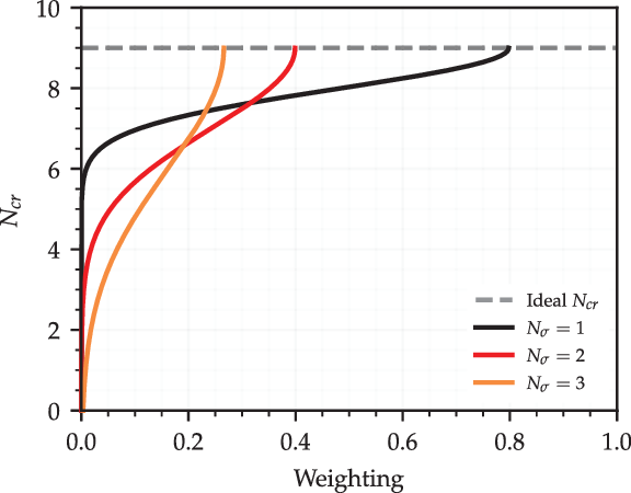
. Figure 1 shows three example negative half-normal
 $N_{cr}$
probability distributions. Each has the same ideal
 $N_{cr}$
(
 $N_i$
) but different standard deviations of
 $N_{cr}$
(
 $N_\sigma$
). The negative half-normal distribution is represented by the probability density function
 $P(N_{cr})$
shown in Equation (1).
 \begin{equation}P(N_{cr}) = \frac{\sqrt{2}}{N_\sigma\sqrt{\pi}}\exp\left({-\frac{(N_{cr} - N_i)^2}{2N_\sigma^2}}\right);\ \ N_{cr} \leq N_i\end{equation}
Examples of negative half-normal
 $\textit{N}_{\textit{cr}}$
probability distributions with the same ideal
 $\textit{N}_{\textit{cr}}$
but different standard deviations in
 $\textit{N}_{\textit{cr}}$
(
 $\textit{N}_\sigma$
).

It should be noted that it may not always be appropriate to ignore the probability of
 $N_{cr}$
increasing. Rashad and Zingg(Reference Rashad and Zingg9) found that operating an aerofoil at a higher
 $N_{cr}$
than it was designed for could result in laminar separation of the flow and a significant drop in performance. Thus, a skewed distribution may be more appropriate if the probability of
 $N_{cr} > N_i$
is significant. However, as the intuitive analysis of the uncertainty sources carried out by those authors suggests that the probability of
 $N_{cr} > N_i$
is very low, this has not been used for this study.
2.2 Uncertainty propagation and quantification
A sampling-based approach has been used to propagate the uncertainty in
 $N_{cr}$
through the aerodynamic model. Aerofoil designs are evaluated with different
 $N_{cr}$
values sampled at regular intervals over the range of possible values. The results of each evaluation are weighted by the probability of that
 $N_{cr}$
value occurring. The uncertainty in the results is then quantified by taking the standard deviation of these weighted values.
The standard deviation
 $F_\sigma$
of an output variable
 $F(N_{cr})$
is calculated using Equation (2), where
 $k_r$
is the number of
 $N_{cr}$
samples used,
 $F_\mu$
is the weighted mean of the output variable
 $F(N_{cr})$
calculated using Equation (3) and W is the sum of the probability weights found using Equation (4).
 $P(N_{cr})$
is the probability weighting calculated using Equation (1). The term
 $F_\sigma$
is therefore a measure of how much some output variable
 $F(N_{cr})$
varies with uncertainty in
 $N_{cr}$
. Reducing
 $F_\sigma$
thus improves the robustness of the output variable to this uncertainty.
 \begin{eqnarray}F_\sigma = \sqrt{\frac{1}{W}\sum^{k_r}_{j=1}\left[F(N_{cr_j})-F_\mu\right]^2}\end{eqnarray}
 \begin{eqnarray} F_\mu = \frac{1}{W}\sum\limits_{j=1}^{k_r}P(N_{cr_j})F(N_{cr_j}) \end{eqnarray}
 \begin{eqnarray}W = \sum\limits_{j=1}^{k_r}P(N_{cr_j})\end{eqnarray}
The benefit of using uniformly distributed weighted samples over a random sampling method such as Monte Carlo is that far fewer sample points are needed. This is because the evenly spaced samples have perfect equidistribution. This reduces the computational cost, as each sample point represents a model evaluation. The spacing between
 $N_{cr}$
sample points determines the accuracy of the mean and standard deviation values calculated.
However, given the periodic nature of this sampling strategy, it is unsuitable for models exhibiting oscillatory behaviour at a frequency close to that of the samples. In most cases, this will not be an issue as the transition location on both the upper and lower aerofoil surfaces will move monotonically upstream as
 $N_{cr}$
is reduced. However, some oscillations in transition location may be seen as
 $N_{cr}$
is reduced if laminar separation is present. In these cases, the transition location would move upstream of the separation point as
 $N_{cr}$
is reduced. The separation point may then move downstream as turbulent flow can more easily resist flow separation. The resulting lift increase would allow for the same lift coefficient to be maintained at a lower incidence angle. This would in turn result in a more positive pressure gradient on the upper surface, which helps to suppress instability growth and so will move the transition location downstream. In these cases, the accuracy of the uncertainty quantification carried out may be low if an insufficient number of
 $N_{cr}$
samples are used.
2.3 Computational solvers
Two efficient flow solvers were used during this study. The first, used for analysis and optimisation at subsonic conditions, was XFOIL, developed by Drela(Reference Drela and Mueller26). This is a 2D flow analysis tool which uses the viscous–inviscid interaction (VII) approach to couple a potential flow panel method with an integral boundary-layer solution and a simplified incompressible
 $e^N$
transition model(Reference Drela and Giles27). Additional corrections are included to account for weak compressibility effects and mild separation. Simulations were run with 300 panels during this study, which is near the maximum allowed by XFOIL. This was done to ensure that the results were independent of the number of panels used. While XFOIL is considered to be a low-fidelity solver given its use of VII over the Reynolds-averaged Navier–Stokes approach, it is a highly reliable tool when operated within its limitations and has been used extensively in industry.
For analysis and optimisation at transonic conditions, the CVGK flow solver(Reference Atkin and Gowree28) was used. This is derived from BVGK, which was developed by the ex-Royal Aircraft Establishment. CVGK also uses a VII approach(Reference Lock and Williams29), modelling inviscid flow using the Garabedian and Korn(Reference Garabedian and Korn30) (G&K) full potential flow method (with additional improvements as outlined by Lock(Reference Lock31)) and viscous flow using the lag-entrainment integral method(Reference Green, Weeks and Brooman32). This has been coupled with an
 $e^N$
transition model(Reference Atkin33) capable of both incompressible and compressible stability analyses. The compressible
 $e^N$
method is used throughout this work. CVGK is able to model un-swept, infinity swept and swept–tapered wings. As such, it allows for the specification of both Tollmien–Schlichting and crossflow instability
 $N_{cr}$
values. CVGK has been extensively used for transonic wing design in the UK aerospace industry and validated at swept and un-swept transonic flow conditions(Reference Atkin and Gowree28,Reference Gowree34) . Atkin and Gowree(Reference Atkin and Gowree28) found good agreement between computational results from CVGK and wind-tunnel results for the RAE5237 and RAE5240 from
 $0.6<\text{M}<0.85$
. It was, however, found that CVGK slightly under-estimated the shock strength at high Mach numbers. CVGK was found to produce mesh-independent results over the Mach range investigated with 240 cells in the stream-wise direction and 48 in the wall-normal direction. To increase the transition location accuracy during this study, 320 cells were used in the stream-wise direction for all simulations.
3.0 CRITICAL N-FACTOR UNCERTAINTY ANALYSIS
3.1 Definition of subsonic problem
The NLF0215 aerofoil(Reference Somers35) has been analysed using the proposed methodology to investigate how its performance varies with uncertainty in
 $N_{cr}$
. This is a flapped aerofoil developed for low drag at a cruise lift coefficient of
 $C_l=0.2$
and climb lift coefficient range of
 $0.5<C_l<1.0$
. The design Reynolds number and Mach number were
 $\text{Re}=9\times10^6$
and
 $\text{M}=0.1$
. A fixed flap deflection angle of
 $0^\circ$
is used during this study. Analysis of the aerofoil is carried out at the cruise Reynolds number of
 $\text{Re}=9\times10^6$
and Mach number of
 $\text{M}=0.1$
over the lift coefficient range of
 $0\leq C_l \leq1.6$
with the angle-of-attack left free. Practical implementation of NLF will require some form of protection from leading-edge contamination(Reference Wicke, Linke, Gollnick and Kruse36). It is assumed that a method such as liquid discharge(Reference Young and Humphreys6) can be used for subsonic applications. This approach protects both the upper and lower surfaces from contamination, so the transition is left free on both during this study.
The probability distribution describing the uncertainty in
 $N_{cr}$
has an ideal value of
 $N_i=9$
and a standard deviation of
 $N_\sigma=2$
.
 $N_i=9$
is selected as the simplified
 $e^N$
model in XFOIL is based on the
 $e^9$
method of Smith and Gamberoni(Reference Smith and Gamberoni37). This value is also used in other studies on aerofoil performance at similar flow conditions(Reference Drela38,Reference Driver and Zingg39,Reference Rashad and Zingg9) . The value of
 $N_\sigma$
is selected somewhat arbitrarily, and so the effect of varying
 $N_\sigma$
is also included in the analysis. The mean performance and standard deviation of the performance of the aerofoil are calculated at each lift coefficient. This is done using flow solutions evaluated with
 $N_{cr}$
values taken in steps of
 $0.1$
from
 $N_{cr}=9\to0$
.
3.2 Subsonic analysis
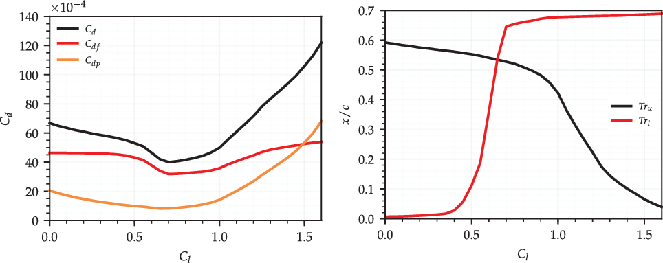
Figure 2 shows the drag and transition polars of the NLF0215 when
 $N_{cr}=9$
. The drag polar includes the total drag (
 $C_d$
) with the skin friction (
 $C_{df}$
) and pressure drag (
 $C_{dp}$
) components. The transition polar includes the upper-surface (
 $Tr_u$
) and lower-surface (
 $Tr_l$
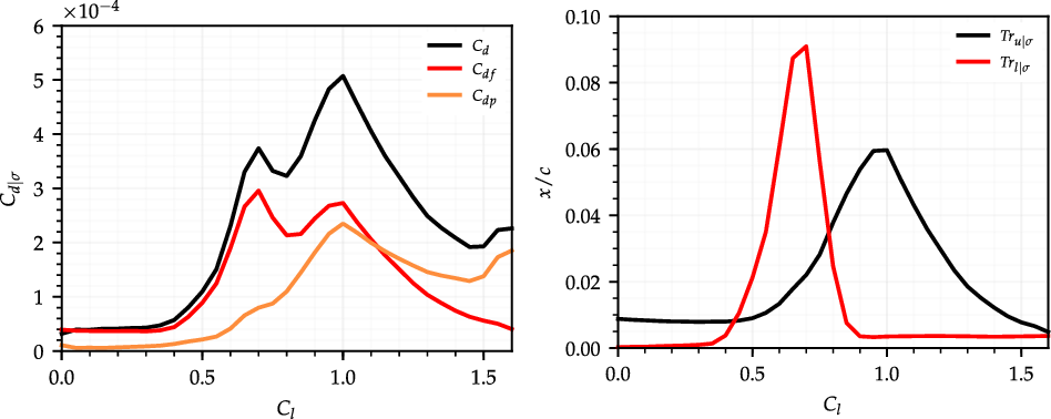
) transition locations. Figure 3 shows the standard deviation of the drag components and transition locations with uncertainty in
 $N_{cr}$
. The standard deviation of each variable is represented by the subscript
 $\sigma$
.
Drag and transition location polars for the NLF0215 when
 $\textit{N}_{\textit{cr}}=\text{9}$
.

Standard deviation of drag and and transition location polars for the NLF0215.

The total drag polar exhibits a bucket shape between
 $0.5 < C_l <1.0$
. This is a common feature of NLF aerofoil designs, where laminar flow is extended on both surfaces through the design lift coefficient range but is quickly lost when moving off-design.
 $Tr_\sigma$
is largest on each surface where the transition location is most sensitive to the lift coefficient. As the peaks in
 $Tr_{u|\sigma}$
and
 $Tr_{l|\sigma}$
overlap,
 $C_{d|\sigma}$
is high through the entire drag bucket lift coefficient range. Although the peak in
 $Tr_\sigma$
for the upper surface is smaller, the corresponding peak in
 $C_{d|\sigma}$
is larger. This is because a change in the upper-surface transition location has a stronger effect on the lift coefficient. As the angle-of-attack is varied to obtain the desired lift coefficient, this causes both the skin friction and pressure drag to vary. The standard deviation of
 $C_d$
is larger as a result. The sensitivity of the pressure drag to the lift coefficient is larger at higher lift coefficients. This is apparent in the
 $C_{d|\sigma}$
polar, where the standard deviation of
 $C_{dp}$
is large at high lift coefficients while
 $Tr_\sigma$
is low for both surfaces. The
 $C_{d|\sigma}$
polar therefore takes the shape of the combined
 $Tr_\sigma$
polars at low lift coefficient values, but diverges from this as the lift coefficient is increased.
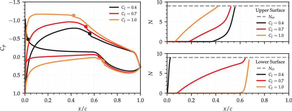
Figure 4 shows the pressure distributions and N-factor envelopes for the NLF0215 at lift coefficients of
 $C_l=0.4$
,
 $C_l=0.7$
and
 $C_l=1.0$
when
 $N_{cr}=9$
. These help to explain why
 $Tr_\sigma$
is largest on each surface when the transition location at the ideal
 $N_{cr}$
is most sensitive to changes in the lift coefficient. A strong adverse pressure gradient on both surfaces at
 $C_l=0.4$
precedes transition. Varying the lift coefficient has little effect on the transition location, as the strength and direction of the pressure gradient are largely unaffected. The lower-surface transition is close to the leading edge and so also insensitive to
 $N_{cr}$
. The upper-surface transition follows a long favourable pressure gradient that suppresses instability growth until rapid growth occurs just upstream of the transition point. Transition is therefore insensitive to reductions in
 $N_{cr}$
until
 $N_{cr}$
is reduced significantly. A weak pressure gradient precedes the transition on the lower surface at
 $C_l=0.7$
and on the upper surface at
 $C_l=1.0$
. Varying the lift coefficient now has a large effect on the transition location, as the direction of the pressure gradient can change over a large chord length. The weak pressure gradient also promotes gradual instability growth up to the transition location. Therefore, only a small reduction in
 $N_{cr}$
is needed to shift the transition upstream.
Pressure distributions and N-factor envelopes for the NLF0215 at
 $\textit{C}_{\textit{l}}=\text{0.4}$
,
 $\text{0.7}$
and
 $\text{1.0}$
with
 $\textit{N}_{\textit{cr}}=\text{9}$
. Markers on the pressure distributions indicate transition locations.

The shape of the
 $C_{d|\sigma}$
and
 $Tr_\sigma$
polars can therefore be inferred from the drag and transition polars found at the ideal
 $N_{cr}$
.
 $Tr_\sigma$
is found to be directly related to the rate of change of the transition location with the lift coefficient at the ideal
 $N_{cr}$
, and
 $C_{d|\sigma}$
is proportional to the sum of the upper- and lower-surface
 $Tr_\sigma$
. It is important to note that this may not hold if a different
 $N_{cr}$
uncertainty distribution or standard deviation of
 $N_{cr}$
is selected. The uncertainty distribution chosen gives the highest probability weighting to the ideal
 $N_{cr}$
. Therefore, the sensitivity of the transition locations to changes in the lift coefficient at the ideal
 $N_{cr}$
has the greatest effect on
 $Tr_\sigma$
. This relationship will diminish if the probability weighting at the ideal
 $N_{cr}$
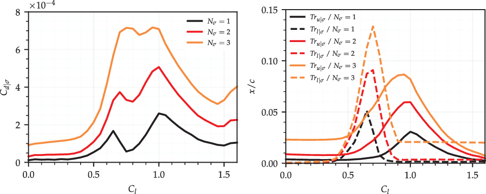
is reduced. Figure 5 shows the standard deviation of
 $C_d$
and the standard deviation of Tr polars when calculated with different standard deviations of
 $N_{cr}$
(
 $N_\sigma$
).
Standard deviation of drag and transition location polars for the NLF0215 when calculated with different standard deviations of
 $\textit{N}_{\textit{cr}}$
.

 $\textit{ML}/\textit{D}$
, drag and upper-surface transition location polars for the RAE2822 when
 $\textit{N}_{\textit{cr}}=\text{9}$
.

The value of
 $C_{d|\sigma}$
and
 $Tr_\sigma$
grows at all lift coefficients as
 $N_\sigma$
is raised. The increase in
 $Tr_\sigma$
is greatest for each surface where
 $Tr_\sigma$
is already large. However,
 $Tr_\sigma$
increases everywhere where extended laminar flow is achieved at the ideal
 $N_{cr}$
. Regardless of the
 $N_\sigma$
value chosen, the
 $C_{d|\sigma}$
polar still has the same form as the combined
 $Tr_\sigma$
polars at low lift coefficient values. However, the
 $C_{d|\sigma}$
polar deviates more from this at higher lift coefficients if
 $N_\sigma$
is larger.
3.3 Definition of transonic problem
The RAE2822 aerofoil(Reference Cook, McDonald and Firmin40) has also been analysed using the proposed methodology to investigate how its performance varies with uncertainty in
 $N_{cr}$
. This is a supercritical aerofoil designed for
 $C_l=0.56$
at
 $\text{M}=0.66$
with the transition fixed near the leading edge on both surfaces. During this study, the transition remains fixed on the lower surface at
 $0.03x/c$
but is free to move on the upper surface. A popular method for fixing the transition on the lower surface to protect the leading edge from contamination on large transonic aircraft is the use of a Krueger flap(Reference Tamigniaux, Stark and Brune41–Reference van Dam43). This shields the leading edge when deployed during take-off, before being retracted into the lower surface during cruise. This leaves the upper surface free of contamination but triggers an early transition on the lower surface. Initial analysis of the aerofoil at a Reynolds number of
 $\text{Re}=6.5\times10^6$
and
 $N_{cr}=9$
with a free transition on the upper surface found that
 $(ML/D)_{\max}$
occurs at approximately
 $\text{M}=0.715$
and
 $C_l=0.76$
. This is used to fix
 $\text{M}^2C_l$
while varying the Mach number between
 $0.68<\text{M}<0.73$
. The angle-of-attack is varied to obtain the target lift coefficient at each Mach number.
The probability distribution describing the uncertainty in
 $N_{cr}$
again has an ideal value of
 $N_i=9$
and a standard deviation of
 $N_\sigma=2$
.
 $N_i=9$
is selected as it lies between the values of
 $N_{cr}$
obtained from the compressible
 $e^N$
stability analysis of ATTAS and FOKKER 100 NLF flight test data without the presence of crossflow instability growth(Reference Schrauf44,Reference Schmitt, Archambaud, Horstmann and Quast45) .
 $N_\sigma=2$
is again selected somewhat arbitrarily, with the effect of varying
 $N_\sigma$
included in the analysis. The mean performance and the standard deviation in the performance of the aerofoil are calculated at each Mach number–lift coefficient combination. This is again done using flow solutions evaluated with
 $N_{cr}$
values taken at steps of
 $0.1$
from
 $N_{cr}=9\to0$
.
3.4 Transonic analysis
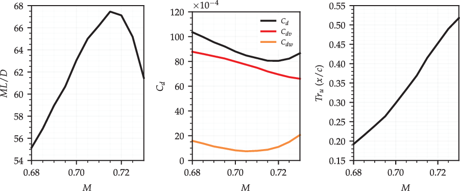
Figure 6 shows the
 $ML/D$
, drag (
 $C_d$
) and upper-surface transition location (
 $Tr_u$
) polars for the RAE2822 when
 $N_{cr}=9$
. The drag polar is broken down into viscous (
 $C_{dv}$
) and wave drag (
 $C_{dw}$
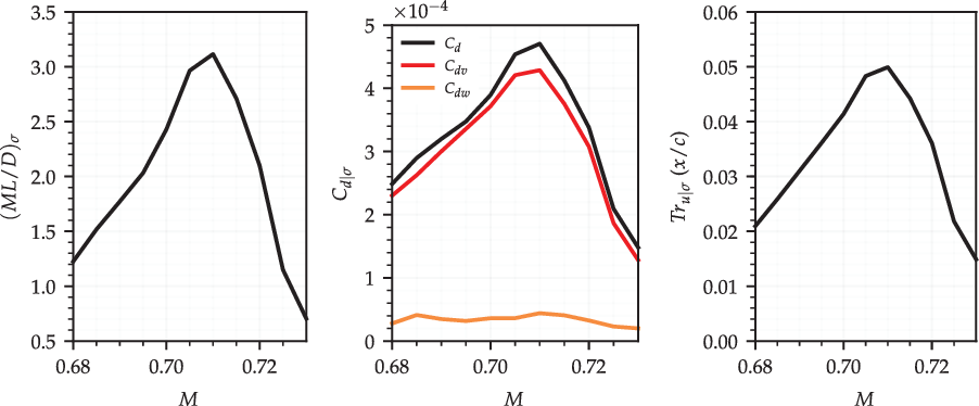
) components. Figure 7 shows the standard deviation of each with uncertainty in
 $N_{cr}$
. The standard deviation is denoted by the subscript
 $\sigma$
.
Standard deviation of
 $\textit{ML}/\textit{D}$
, drag and upper-surface transition location polars for the RAE2822.

The total drag is dominated by the viscous drag component at the ideal
 $N_{cr}$
for the considered Mach number range. As
 $\text{M}^2C_l$
is fixed, increasing the Mach number reduces the lift coefficient and the angle-of-attack. This leads to a near-linear reduction in the viscous drag as the transition location moves downstream. The maximum
 $ML/D$
coincides with the minimum drag. This occurs at the point where increasing the Mach number causes a rise in the wave drag that outweighs the reduction in the viscous drag.
 $(ML/D)_\sigma$
and
 $C_{d|\sigma}$
are both largest at a Mach number just below this. As the total drag is dominated by the viscous drag component, the
 $C_{d|\sigma}$
and
 $Tr_{u|\sigma}$
polars are very similar.
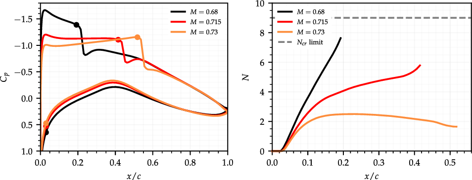
The shape of the
 $Tr_{u|\sigma}$
polar can be explained using Fig. 8 showing the pressure distributions and N-factor envelopes for the RAE2822 at Mach numbers of
 $\text{M}=0.680$
,
 $\text{M}=0.715$
and
 $\text{M}=0.730$
when
 $N_{cr}=9$
. A strong favourable pressure gradient is obtained at the lower end of the Mach number range where the lift coefficient is small. This suppresses instability growth and delays the transition up to the shock position. As instability growth is suppressed, the transition location only moves upstream once
 $N_{cr}$
is significantly reduced.
 $Tr_{u|\sigma}$
is therefore small. A strong adverse pressure gradient is obtained at the upper end of the Mach number range where the lift coefficient is large. Although this causes upstream instability growth, the transition at the ideal
 $N_{cr}$
occurs closer to the leading edge, so reducing
 $N_{cr}$
can only lead to a small reduction in laminar flow.
 $Tr_{u|\sigma}$
is therefore small. In both cases,
 $Tr_\sigma$
is small when the transition is shock induced at the ideal
 $N_{cr}$
, as reducing
 $N_{cr}$
has no initial effect on the transition location. All three N-factor envelopes shown end at the point of shock-induced transition and so fail to reach
 $N_{cr}=9$
.
Pressure distributions and N-factor envelopes for the RAE2822 at
 $\text{M}=\text{0.680}$
,
 $\text{0.715}$
and
 $\text{0.730}$
with
 $\textit{N}_{\textit{cr}}=\text{9}$
. Markers on the pressure distributions indicate transition locations.

The effect that the standard deviation of
 $N_{cr}$
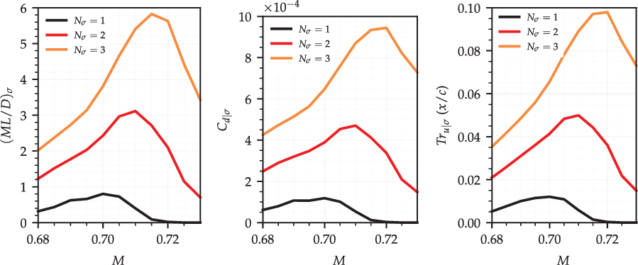
uncertainty has on the aerofoil performance is again assessed. Figure 9 shows the
 $(ML/D)_\sigma$
,
 $C_{d|\sigma}$
and
 $Tr_{u|\sigma}$
polars when calculated with different standard deviations of
 $N_{cr}$
uncertainty. As expected, all three standard deviation polars grow in magnitude as
 $N_\sigma$
is increased. The increase is comparable between the polars and largest at higher Mach numbers, as this is where there is the largest amount of laminar flow at the ideal
 $N_{cr}$
. If there is a larger amount of laminar flow at the ideal
 $N_{cr}$
, a larger amount is lost as
 $N_{cr}$
is reduced from the ideal value to zero. If there is strong instability suppression, this shift in the transition location will occur at small
 $N_{cr}$
values with low probability and have little effect on
 $Tr_\sigma$
. However, the probability only needs to increase slightly for this loss of laminar flow to have a much larger effect on the calculated
 $Tr_\sigma$
.
Standard deviation of
 $\textit{ML}/\textit{D}$
, drag and upper-surface transition location polars for the RAE2822 when calculated with different standard deviations of
 $\textit{N}_{\textit{cr}}$
uncertainty.

4.0 ROBUST OPTIMISATION
4.1 Problem formulation
Two multi-objective shape optimisation cases have been considered. The goal of each was to improve the aerofoil performance with uncertainty in
 $N_{cr}$
. The NLF0215 aerofoil with a fixed flap deflection angle of
 $0^\circ$
is used as a starting shape for a subsonic optimisation case. This is optimised at a Reynolds number of
 $\text{Re}=9\times10^6$
, Mach number of
 $\text{M}=0.1$
and lift coefficient of
 $C_l=0.7$
. The optimisation objectives used are minimisation of the mean drag and the standard deviation of the drag with uncertainty in
 $N_{cr}$
. The angle-of-attack is left free for the flow solver to control so that the target lift coefficient can be obtained. The transition is left free on both surfaces.
The RAE2822 aerofoil is used as the starting shape for a transonic optimisation case. This is optimised at a Reynolds number of
 $\text{Re}=6.5\times10^6$
, Mach number of
 $\text{M}=0.715$
and lift coefficient of
 $C_l=0.76$
. The optimisation objectives used are maximisation of the mean
 $ML/D$
and minimisation of the standard deviation of
 $ML/D$
with uncertainty in
 $N_{cr}$
. The angle-of-attack is again left free for the flow solver to control. The transition is left free on the upper surface but is fixed at
 $0.03x/c$
on the lower surface.
The mean performance and the standard deviation of the performance are calculated using the proposed uncertainty quantification method in both cases. The probability distribution describing the uncertainty in
 $N_{cr}$
has an ideal value of
 $N_i=9$
and a standard deviation of
 $N_\sigma=2$
, matching the values used during the uncertainty analysis. The optimiser changes the aerofoil shape using 6 design variables per surface for a total of 12. These come from the selected parameterisation method discussed in detail below. Bounds are placed on each design variable so that the optimiser has a finite design space to explore. The selection of these are also outlined below. Both cases have a constraint placed on the maximum aerofoil thickness, ensuring that all the optimised designs have a maximum thickness that is larger than or equal to that of the starting aerofoil.
A Python-based genetic algorithm is used to conduct the optimisation. This is implemented using the Distributed Evolutionary Algorithms in Python (DEAP) package(Reference Fortin, Rainville, Gardner, Parizeau and GagnÉ46) and interfaces with the external flow solver used in each case. Genetic algorithms replicate the selection, mating and mutation processes found in natural evolution, creating successive generations of new designs that combine the favourable characteristics of their predecessors. Initial designs are generated randomly within the design variable bounds and checked against the geometric constraints before being evaluated. Designs from this initial generation are selected using the NSGA-2 non-dominated method(Reference Deb, Pratap, Agarwal and Meyarivan47), mated using simulated binary crossover(Reference Deb and Agrawal48) and mutated using the bound polynomial mutation method(Reference Deb and Agrawal49). New designs obtained through this process are then evaluated. This is repeated until a limit on the number of generations to evaluate is reached.
4.2 Parameterisation
There are various approaches to aerofoil parameterisation that can be grouped into two distinct categories: constructive and deformative(Reference Masters, Taylor, Rendall, Allen and Poole50). Constructive methods define the aerofoil shape itself, while deformative methods define a perturbation profile which is then used to deform a starting aerofoil shape. A deformation approach is used in this study as it allows for optimisation of a complex starting aerofoil using a small number of design variables. When using a genetic algorithm, the number of designs needed per generation is between two and ten times the number of design variables used(Reference Alander51,Reference Storn52) . It is, therefore, desirable to use a small number of design variables.
New aerofoil shapes are obtained by changing the z coordinate of a starting aerofoil by some amount defined using a perturbation profile. This is represented mathematically in Equation (5), where
 $z_o$
is the original aerofoil z coordinate and
 $z_p$
is the perturbation z coordinate. u is the chord length position
 $x/c$
.
 \begin{equation}z(u) = z_o(u) + z_p(u)\end{equation}
The perturbation profile is parameterised using the Class Shape Transformation (CST) method developed by Kulfan(Reference Kulfan53). This is shown in Equation (6), where
 $\Delta_{z_{te}}$
is the trailing-edge thickness while C(u) and S(u) are the class and shape functions from the CST method.
 \begin{equation}z_p(u) = C(u)\ S(u) + \left(u\ \Delta_{z_{te}} \right)\end{equation}
The class function is defined in Equation (7), where
 $n_1$
and
 $n_2$
are exponents that determine the basic shape of the CST fitting. The values
 $n_1=0.5$
and
 $n_2=1.0$
are used to define a round-nosed aerofoil with finite trailing-edge gradient as the CST is commonly used for constructive aerofoil parameterisation. Values of
 $n_1=n_2=1$
are used for this application.
 \begin{equation}C(u) = u^{n_1} \left(1 - u\right)^{n_2}\\ \end{equation}
The shape function given in Equation (8) contains n number of CST coefficients,
 $A_r$
. These are the design variables controlled by the optimiser. As the optimiser varies each of these coefficients, the magnitude of the perturbation profile will change, deforming the original aerofoil and so creating new aerofoil designs. In both the subsonic and transition optimisation cases, six CST coefficients are used to define the perturbation profile on each surface. Therefore, the optimiser is in control of 6 design variables per surface, or 12 design variables in total.
 \begin{equation}S(u) = \sum^{n}_{r=0} A_r\ \frac{n!}{r!(n - r)!} u^r \left(1 - u \right)^{n - r}\end{equation}
Upper and lower bounds were placed on the design variables during optimisation. In both cases, these were selected to allow for a large design space to be explored while also attempting to prevent the generation of infeasible designs, which would waste computational resources and slow down the progress of the optimiser.
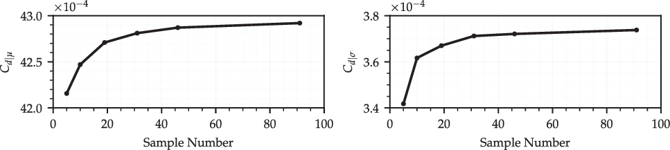
Mean and standard deviation of drag calculated with a varying number of
 $\textit{N}_{\textit{cr}}$
samples for the NLF0215 aerofoil at
 $\textit{C}_{\textit{l}}=\text{0.7}$
,
 $\text{M}=\text{0.1}$
and
 $\text{Re}=\text{9}\times\text{10}^{\text{6}}$
.

4.3 Uncertainty sampling
The number of
 $N_{cr}$
sample points used should be as small as possible while still being sufficient to calculate the mean performance and the standard deviation of the performance of an aerofoil with acceptable accuracy. This is because each sample point requires a flow solution, and so additional sample points increase the computational cost substantially. To determine the minimum number of sample points needed, a sample dependence study has been carried out for both the NLF0215 and RAE2822 aerofoils at the flow conditions to be used during their optimisation. For each aerofoil, a number of
 $N_{cr}$
samples are taken at regular intervals between the ideal
 $N_{cr}=9$
and
 $N_{cr}=0$
. The performance of the aerofoil is calculated at the design Mach number, Reynolds number and lift coefficient with each of the
 $N_{cr}$
values. These are then weighted by the probability of that
 $N_{cr}$
value occurring and used to calculate the mean and standard deviation of the performance with uncertainty in
 $N_{cr}$
. This process is repeated for different numbers of
 $N_{cr}$
samples. The mean and standard deviation of the aerofoil performance can then be plotted against the number of
 $N_{cr}$
samples used, to assess the accuracy obtained as the number of samples is varied.
Figure 10 shows the mean drag and the standard deviation of the drag for the NLF0215 when calculated with different numbers of
 $N_{cr}$
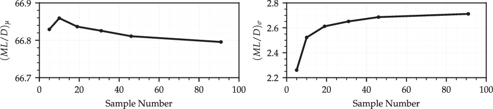
samples. Figure 11 shows the mean
 $ML/D$
and the standard deviation of
 $ML/D$
for the RAE2822 when calculated with different numbers of
 $N_{cr}$
samples. As expected, the mean and standard deviation converge as the number of samples used increases for both cases. The mean drag is within
 $0.4$
% and the standard deviation of the drag is within 2% of the values found using 91 samples when only 19 samples are used for the NLF0215. The mean
 $ML/D$
is within
 $0.003$
% and the standard deviation of
 $ML/D$
is within 3% of the values found using 91 samples when only 19 sample points are used for the RAE2822. Thus, it is felt that 19
 $N_{cr}$
samples taken at intervals of
 $0.5$
over the
 $N_{cr}$
range gives acceptable accuracy while reducing the computational cost as much as possible.
Mean
 $\textit{ML}/\textit{D}$
and standard deviation of
 $\textit{ML}/\textit{D}$
calculated with a varying number of
 $\textit{N}_{\textit{cr}}$
samples for the RAE2822 aerofoil at
 $\textit{C}_{\textit{l}}=\text{0.76}$
,
 $\text{M}=\text{0.715}$
and
 $\text{Re}=\text{6.5}\times\text{10}^{\text{6}}$
.

5.0 RESULTS
5.1 Subsonic results
The optimisation produced 4,800 unique designs before the 100 generations limit. XFOIL was able to converge 3,051 of these at all
 $N_{cr}$
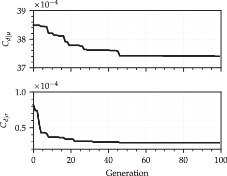
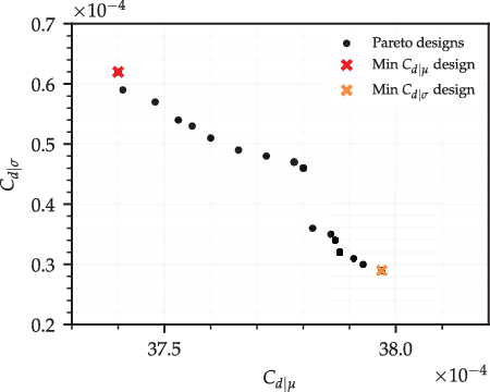
sample points. Figure 12 shows the minimum mean drag (
 $C_{d|\mu}$
) and the standard deviation of the drag (
 $C_{d|\sigma}$
) found during the optimisation. After approximately 50 generations, the value of each is close to the final value found. Further iterations therefore primarily serve to explore the trade-off between objectives. Figure 13 shows designs on the Pareto front found between the two objective functions. All designs are at least 2 mean drag counts lower than the NLF0215 at the chosen design conditions and have a 3 drag count or more decrease in the standard deviation of the drag. The optimised aerofoils with the smallest
 $C_{d|\mu}$
and
 $C_{d|\sigma}$
are also indicated on the Pareto front. These are selected for comparison against the NLF0215, and are denoted as design M (standing for minimum mean drag) and design S (standing for minimum standard deviation of drag).
Minimum mean drag and standard deviation of drag found during the optimisation.

Mean drag and standard deviation of drag for Pareto-front aerofoil designs.

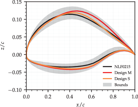
Figure 14 shows aerofoil profiles for the NLF0215 and selected optimised designs. The grey-shaded area indicates the viable design region as dictated by the design variable bounds. Both optimised aerofoils have common NLF design characteristics such as an increased maximum thickness located further aft and an increased curvature at the leading edge of the upper surface followed by a reduced curvature between
 $0.05<x/c<0.4$
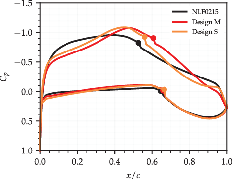
. In combination, this creates a more favourable pressure gradient which thus delays the transition. This can be seen in Fig. 15, which shows the pressure distributions for the NLF0215 and selected optimised designs at the ideal
 $N_{cr}$
of
 $N_{cr}=9$
. Some differences are seen between the two optimised designs despite their similar
 $C_{d|\mu}$
and
 $C_{d|\sigma}$
values. Design M is thicker than design S towards the rear of the aerofoil and so requires a smaller angle-of-attack to generate the same lift. This results in a longer upper-surface favourable pressure gradient and so more laminar flow. The smaller angle-of-attack has little effect on the lower-surface pressure gradient.
Aerofoil profiles for the NLF0215 and selected optimised designs.

Pressure distributions for the NLF0215 and selected optimised designs at
 $\textit{N}_{\textit{cr}}=\text{9}$
. Markers indicate transition location.

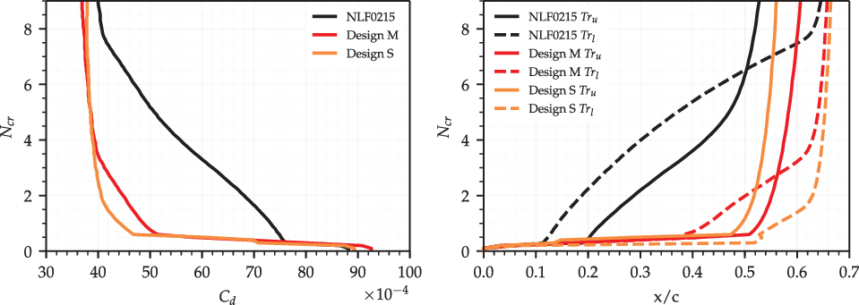
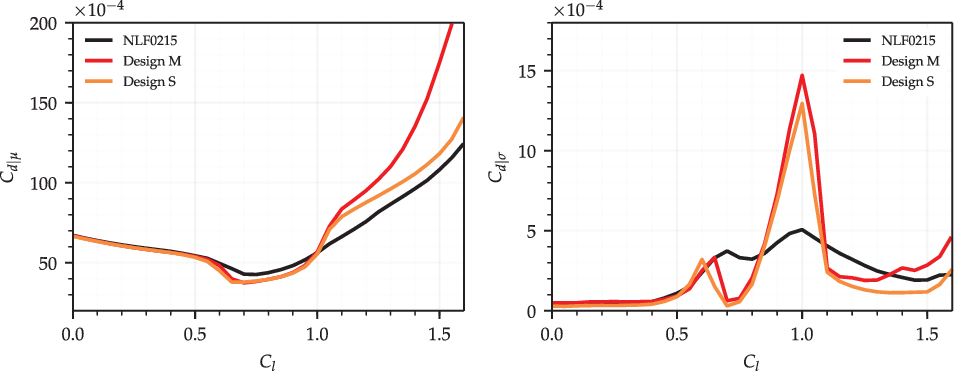
Figure 16 shows the drag and transition locations with varying
 $N_{cr}$
for the NLF0215 and selected optimised designs. These were obtained using
 $N_{cr}$
samples taken at intervals of
 $0.1$
as done during the uncertainty analysis carried out previously. As expected, both optimised designs have lower drag than the NLF0215 over almost all of the
 $N_{cr}$
range. The reduction in drag is small at the ideal
 $N_{cr}$
but becomes much greater as
 $N_{cr}$
is reduced. While both optimised designs have only a slightly delayed transition at the ideal
 $N_{cr}$
on each surface, this is maintained down to much smaller
 $N_{cr}$
values.
Variation of drag and transition locations with changes in
 $\textit{N}_{\textit{cr}}$
for the NLF0215 and selected optimised designs.

To delay the transition at the ideal
 $N_{cr}$
, the favourable pressure gradient up to the transition location should be as long as possible. However, its strength must be weak to avoid flow separation caused by the strong adverse pressure that will inevitably follow it. A weak favourable pressure gradient will delay the transition at the ideal
 $N_{cr}$
but see stronger upstream instability growth. It will therefore be more sensitive to the lift coefficient and
 $N_{cr}$
. A shorter but stronger favourable pressure gradient has the inverse effect. This can be seen in the differences between designs M and S. A more favourable pressure gradient up to the location of minimum pressure helps design S keep
 $Tr_l$
extended down to lower
 $N_{cr}$
values. A stronger adverse pressure gradient past the location of minimum pressure moves the transition at the ideal
 $N_{cr}$
upstream compared with design M, but this also reduces the sensitivity of
 $Tr_u$
to
 $N_{cr}$
at high
 $N_{cr}$
values. Both effects combine to reduce
 $C_{d|\sigma}$
.
Off-design analysis of the selected optimised aerofoils has also been carried out. Figure 17 shows
 $C_{d|\mu}$
and
 $C_{d|\sigma}$
for the NLF0215 and selected optimised designs at a range of lift coefficients. The analysis carried out previously showed that the standard deviation of the transition location, and thus drag, is smallest when the sensitivity of the transition location to the lift coefficient at the ideal
 $N_{cr}$
is low. As the selected optimised designs have a reduced
 $C_{d|\sigma}$
at the design lift coefficient, the sensitivity of
 $C_{d|\mu}$
to the lift coefficient at the design lift coefficient is also low. By reducing both
 $C_{d|\sigma}$
and
 $C_{d|\mu}$
, a reduction in
 $C_{d|\mu}$
is achieved between
 $C_l=0.65$
and
 $1.0$
using only a single lift coefficient design point. However, both designs do now feature strong drag bucket shapes and higher mean drag than the NLF0215 above
 $C_l=1.0$
.
 $C_{d|\sigma}$
also peaks at the upper end of the
 $C_{d|\sigma}$
bucket lift coefficient range. The analysis carried out previously showed that a more rapid movement of the transition location over a smaller lift coefficient range at the ideal
 $N_{cr}$
resulted in a larger peak in the standard deviation of the transition location, and thus drag. The larger peak in
 $C_{d|\sigma}$
at
 $C_l=1.0$
seen with both optimised designs comes from this larger movement of the transition location over a smaller lift coefficient range. These results indicate that aerofoil designs that are insensitive to changes in
 $N_{cr}$
and so changes in the lift coefficient on-design become more sensitive off-design to both.
Mean drag and standard deviation of drag polars for the NLF0215 and selected optimised designs.

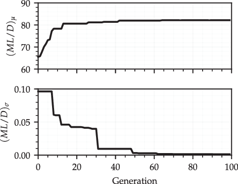
Minimum value found for mean
 $\textit{ML}/\textit{D}$
and standard deviation of
 $\textit{ML}/\textit{D}$
during optimisation.

5.2 Transonic results
The optimisation produced 4,800 unique designs before the 100 generations limit. CVGK was able to converge 1,504 of these at all
 $N_{cr}$
sample points. Figure 18 shows the minimum mean
 $ML/D$
(
 $(ML/D)_\mu$
) and the standard deviation of
 $ML/D$
(
 $(ML/D)_\sigma$
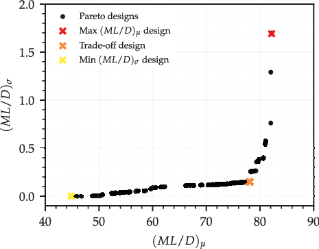
) found during the optimisation. Neither objectives improve after 70 iterations, which suggests an optimum of each is found. The Pareto front found between the objects is shown in Fig. 19. All Pareto-front designs have a lower
 $(ML/D)_\sigma$
than the RAE2822, but some designs only achieve this with a smaller
 $(ML/D)_\mu$
. The maximum
 $(ML/D)_\mu$
found is much larger than for the RAE2822. A reduction in
 $(ML/D)_\sigma$
can be obtained by allowing a small decrease in
 $(ML/D)_\mu$
, but reducing
 $(ML/D)_\sigma$
further then results in a substantial drop in
 $(ML/D)_\mu$
. The optimised designs with maximum
 $(ML/D)_\mu$
, minimum
 $(ML/D)_\sigma$
and an aerofoil trading off between the two variables are also highlighted in Fig. 19 and selected for comparison against the RAE2822. These are denoted design M (standing for maximum mean
 $ML/D$
), design S (standing for minimum standard deviation of
 $ML/D$
) and design T (standing for a trade-off between the objectives).
Mean
 $\textit{ML}/\textit{D}$
and standard deviation of
 $\textit{ML}/\textit{D}$
for Pareto-front designs.

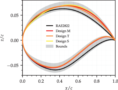
Aerofoil profiles for the RAE2822 and selected optimised designs are shown in Fig. 20, with the grey-shaded area indicating the viable design region dictated by the design variable bounds. The optimised aerofoils have an increased camber compared with the RAE2822. The increase is largest at the trailing edge to help lower the angle-of-attack required to obtain the target lift coefficient. The leading-edge curvature is increased for designs M and T but reduced for design S. Figure 21 shows the pressure distributions for the RAE2822 and selected optimised aerofoils at the ideal
 $N_{cr}=9$
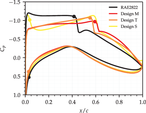
. The reduced angle-of-attack and increased leading-edge curvature result in a long favourable pressure gradient for designs M and T. This extended the laminar flow on the upper surface of both designs by delaying the shock position, while also helping to suppress instability growth. Design M is slightly thicker than design T and so operates at a lower angle-of-attack. As such, it is able to obtain a weaker and more delayed shock. In contrast to this, design S has an increased leading-edge curvature and so sees a strong shock and earlier transition close to the leading edge.
Aerofoil profiles for the RAE2822 and selected optimised designs.

Pressure distributions for the RAE2822 and selected optimised designs.

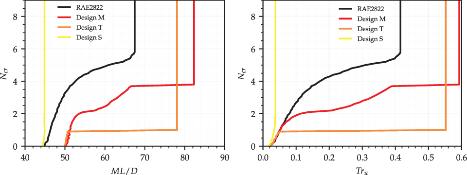
Figure 22 shows how
 $ML/D$
and
 $Tr_u$
vary with
 $N_{cr}$
for the RAE2822 and selected optimised design. All the designs see no change in
 $ML/D$
until
 $N_{cr}<6$
, as the low instability amplification means that the upper-surface transition is shock induced. Both designs M and T have a higher
 $ML/D$
than the RAE2822 over the entire
 $N_{cr}$
range. Laminar flow has been extended on both designs by moving the shock position downstream. Laminar flow is maintained on both designs at lower
 $N_{cr}$
values due to the stronger favourable pressure gradient obtained. The
 $N_{cr}$
value where the instability-induced transition first occurs is lower for design T than design M as the favourable pressure gradient obtained is stronger. However, design T has a lower maximum
 $ML/D$
than design M as this causes a stronger shock positioned further upstream. Fixing the transition near the leading edge at
 $N_{cr}=9$
means that design S sees almost no change in
 $ML/D$
as
 $N_{cr}$
is reduced. While this design has a very low
 $(ML/D)_\sigma$
, it is of no practical use to a designer given its extremely low
 $(ML/D)_\mu$
. The transition location envelope closely matches the
 $ML/D$
envelope for all the designs when
 $N_{cr}>2$
. Designs M and T have higher
 $ML/D$
below
 $N_{cr}=2$
, indicating that they perform better than the RAE2822 under turbulent conditions.
Variation of
 $\textit{ML}/\textit{D}$
and upper-surface transition location with changes in
 $\textit{N}_{\textit{cr}}$
for the RAE2822 and selected optimised aerofoils.

Off-design analysis of designs M and T has also been performed for comparison against the RAE2822. Design S was excluded due to its poor
 $(ML/D)_\mu$
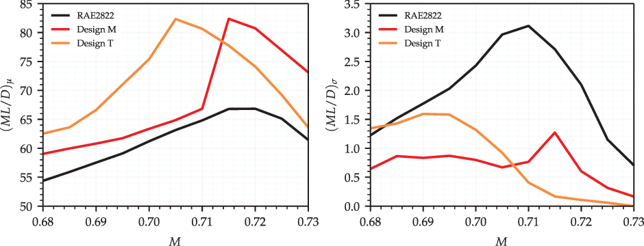
value. Figure 23 shows the
 $(ML/D)_\mu$
and
 $(ML/D)_\sigma$
polars for the RAE2822 and selected optimised designs at a range of Mach numbers. Both optimised designs have a larger
 $(ML/D)_\mu$
and smaller
 $(ML/D)_\sigma$
than the RAE2822 over the entire Mach number range investigated. Design M has the largest
 $(ML/D)_\mu$
above the design Mach number. This is due to its having a weaker but longer favourable pressure gradient and so most delayed shock position. The stronger but shorter favourable pressure gradient of design T results in an earlier shock but better instability suppression at high Mach numbers. Design M sees a large reduction in
 $(ML/D)_\mu$
below the design Mach number. This is due to a sudden upstream movement of the transition location at the ideal
 $N_{cr}$
triggered by the laminar boundary-layer solver detecting flow separation in the presence of a strong adverse pressure gradient. As less laminar flow is obtained, design M also sees a reduction in
 $(ML/D)_\sigma$
. As design T features a stronger favourable pressure gradient at the design Mach number, the transition location is slower to move upstream as the Mach number is reduced, and laminar boundary-layer separation is not detected until below
 $\text{M}=0.705$
. Design T does, however, see an increase in
 $(ML/D)_\sigma$
as the Mach number is reduced. As
 $\text{M}^2C_l$
is fixed, reducing the Mach number increases the lift coefficient and so the angle-of-attack. This results in a less favourable and more adverse pressure gradient that promotes upstream instability growth.
Mean
 $\textit{ML}/\textit{D}$
and standard deviation of
 $\textit{ML}/\textit{D}$
polars for the RAE2822 and selected optimised aerofoils.

It is important to note that the transition location oscillates substantially during the convergence of cases with laminar separation. A much stronger under-relaxation of the transition location and an increased iteration limit not specified during the optimisation was needed to converge these cases. As such, a uniformly spaced sampling method for uncertainty propagation may not be appropriate when laminar separation is encountered. Furthermore, CVGK is not able to model laminar separation bubbles or re-lamination of the boundary layer, which may be occurring for these cases. These limitations are not, however, felt to affect the validity of the trends observed.
6.0 CONCLUSIONS
The effect of uncertainty in the critical N-factor (
 $N_{cr}$
) on the performance and shape optimisation of natural laminar flow aerofoils has been investigated. Uncertainty in
 $N_{cr}$
can be attributed to a degradation in the surface and flow quality, which is not directly modelled but assumed to be crudely incorporated through a reduction in
 $N_{cr}$
. Uncertainty in
 $N_{cr}$
is modelled using a negative half-normal probability distribution.
Analysis of the NLF0215 aerofoil showed that the standard deviation of the transition location caused by uncertainty in
 $N_{cr}$
is largest when the transition location at the ideal
 $N_{cr}$
is sensitive to changes in the lift coefficient. An estimate of the standard deviation of the transition location with uncertainty in
 $N_{cr}$
can therefore be made using the aerofoil’s transition location polar at the ideal
 $N_{cr}$
. This is beneficial as it allows for an initial prediction of the most uncertain transition polar regions without the use of uncertainty analysis methods. The standard deviation of the drag is proportional to the combined standard deviation of the upper- and lower-surface transition locations at low lift coefficient values. This is not so at high lift coefficients, as even small changes in the upper-surface transition location cause large variations in the pressure drag. Analysis of the RAE2822 showed that the standard deviation of
 $ML/D$
(when
 $\text{M}^2C_l$
is fixed) is proportional to the standard deviation of the upper-surface transition location. The standard deviation of
 $ML/D$
is largest when
 $ML/D$
at the ideal
 $N_{cr}$
is high, and reduces as Mach number is increased and decreased from this point. The transition lies close to the leading edge at low Mach numbers and so is insensitive to
 $N_{cr}$
. A strong favourable pressure gradient suppresses instability growth up to the downstream shock position at high Mach numbers.
Robust shape optimisation of each aerofoil was then carried out with the goal of reducing the mean drag and the standard deviation of the drag for the NLF0215, and increasing the mean
 $ML/D$
and reducing the standard deviation of
 $ML/D$
for the RAE2822. In both cases, the optimiser is able to produce designs that have improved mean performance and a reduced standard deviation of performance with uncertainty in
 $N_{cr}$
at the design conditions. However, a trade-off is found between the two objectives once they are sufficiently reduced. Off-design analysis of several optimised aerofoils showed that improvements in the mean and standard deviation of the performance on-design can both reduce when off-design.
Because of this, further work on this topic could aim to extend the methodology used to allow for robust optimisation with uncertainty in
 $N_{cr}$
at a range of Mach numbers or lift coefficients. As the approach used in this study requires a large number of
 $N_{cr}$
samples per design point, this may be too computationally expensive. Work may need to be done to reduce the computational cost of the optimisation or uncertainty quantification methods to compensate. Any further work should also consider pitching moment, as this increased considerably for the optimised aerofoils generated during this study. These designs will therefore incur a trim drag penalty, which may negate any drag reductions found. Finally, only 2D flow was considered during this study. For transonic aerofoils with wing sweep, three-dimensional cross-flow instabilities become important. As the design requirements for suppression of cross-flow instabilities differ from suppression of Tollmien–Schlichting instabilities, analysis of 3D flows would make for another interesting extension to this work.
ACKNOWLEDGEMENTS
The authors acknowledge financial support from the UK Engineering and Physical Sciences Research Council (EPSRC) and Airbus. The authors would also like to thank James Alderman from Airbus Group Innovations (AGI) for his guidance on aerodynamic design methods used in industry.