Introduction
The fundamental differences in swimming ability of ammonoids remain a central puzzle of cephalopod paleobiology. A practical approach is to observe the first-order costs of pushing the shell through the water, then compare the challenges presented by different shell shapes (e.g., Chamberlain Reference Chamberlain1976; Jacobs Reference Jacobs1992). The actual swimming ability of the animal would depend on many variables, including muscular strength and placement (Doguzhaeva and Mapes Reference Doguzhaeva, Mapes, Klug, Korn, De Baets, Kruta and Mapes2015), volume of jettable water, jet behavior (Packard et al. Reference Packard, Bone and Hignette1980; Chamberlain Reference Chamberlain1990, Reference Chamberlain, Rayner and Wootton1991; Neil and Askew Reference Neil and Askew2018), and soft-tissue arrangement (Chamberlain Reference Chamberlain1980; Jacobs Reference Jacobs1992; Jacobs and Landman Reference Jacobs and Landman1993; Parent et al. Reference Parent, Westermann and Chamberlain2014; Klug et al. Reference Klug, Schweigert, Tischlinger and Pochmann2021). Many ammonoid shells produced ornamentation, from subtle ribs to audacious spines (Arkell et al. Reference Arkell, Kummel, Wright and Arkell1957: fig. 133; Moulton et al. Reference Moulton, Goriely and Chirat2015), subject to varied interpretations and evidence of their impact on locomotion (i.e., Chamberlain and Westermann Reference Chamberlain and Westermann1976; Ward Reference Ward1981). Here, we examine only the first-order costs introduced by the primary conch geometry. Assessing fundamental motility challenges (or advantages) introduced by basic conch shape will allow refined study of relative benefits (or disadvantages) added by secondary variations such as ornament (see Chamberlain and Westermann Reference Chamberlain and Westermann1976), soft-tissue manipulation behavior (O'Dor Reference O'Dor2002; Staaf et al. Reference Staaf, Gilly and Denny2014), and so on. To the first order, the basic costs of pushing a shell through the water are relevant to a range of biological realities, including the animals’ possible swimming speeds (Jacobs Reference Jacobs1992; Seki et al. Reference Seki, Tanabe, Landman and Jacobs2000), and relative metabolic demand (relative to contemporaneous sea life). An independent analysis will allow us a means to return to long-standing hypotheses about specific transitions observed in the ammonoid fossil record and develop more intricate hypotheses building on these outcomes.
Current views of ammonoid ecology hinge on comparison to extant relatives and results from hydrostatic and hydrodynamic analyses. All ammonoids are extinct, and their extant relatives demonstrate the enormous range of biotic traits present among cephalopods generally: body types (shelled or soft, torpedo or round, muscular or flimsy, etc.), sizes (squid hatchlings swim freely at <2 mm sizes [Staaf et al. Reference Staaf, Gilly and Denny2014; Roura et al. Reference Roura, Amor, González, Guerra, Barton and Strugnell2019]; colossal squids reach 6 m length [Rosa et al. Reference Rosa, Lopez, Guerreiro, Bolstad and Xavier2017]), locomotory habits (jet propulsion, fin swimming, and arm swimming; Chamberlain Reference Chamberlain1993), and metabolic rates (Seibel et al. Reference Seibel, Thuesen, Childress and Gorodezky1997; Seibel Reference Seibel2007; Seibel and Drazen Reference Seibel and Drazen2007). These combined variations are so great that size does not predict metabolic demand (Fig. 1): comparing a squid, octopus, and vampire squid, each with a mass of 10 g, will involve metabolic demands spanning two orders of magnitude (Seibel et al. Reference Seibel, Thuesen, Childress and Gorodezky1997; Seibel Reference Seibel2007; Seibel and Drazen Reference Seibel and Drazen2007). Some interpretations suggest that ammonoid metabolic rates were, on the whole, higher than those of extant Nautilus (Tajika et al. Reference Tajika, Landman, Hoffmann, Lemanis, Morimoto, Ifrim and Klug2020). Thus, relying on body size and metabolic relationships among extant relatives alone is insufficient for constraining the potential metabolic rates and ecological capabilities of extinct ammonoids.
The metabolic rates of modern cephalopods (lines and points) expand above and below the typical ranges of ocean typical fish (rightmost shaded polygon), benthic invertebrates (crustaceans and echinoderms, dark polygon), and gelatinous invertebrates (leftmost shaded polygon). The largest squids (Loliginidae, filled blue triangles; Ommastrephidae, open blue triangles) have a similar range of metabolic rates, with decreasing rates found among the Gonatidae (crosses), Octopodidae (inverted triangles), Cranchidae (open circles), Histioteuthidae (dots), Vampyroteuthidae (open squares), and Bolitaenidae (filled squares). Modified from Seibel (Reference Seibel2007) and Seibel and Drazen (Reference Seibel and Drazen2007).

Previous experiments, simulations, and analyses on fossils and models do establish guidelines for constraining ammonoid ecology by estimating energy demands in relation to potential locomotion strategies. Hydrostatic analyses conclude that ammonoids attained near-neutral buoyancy with their gas-filled chambered shell (Hoffmann et al. Reference Hoffmann, Lemanis, Naglik, Klug, Klug, Korn, De Baets, Kruta and Mapes2015; Lemanis et al. Reference Lemanis, Zachow, Fusseis and Hoffmann2015; Naglik et al. Reference Naglik, Rikhtegar and Klug2015, Reference Naglik, Rikhtegar and Klug2016; Tajika et al. Reference Tajika, Naglik, Morimoto, Pascual-Cebrian, Hennhöfer and Klug2015; Peterman et al. Reference Peterman, Ciampaglio, Shell and Yacobucci2019, Reference Peterman, Hebdon, Ciampaglio, Yacobucci, Landman and Linn2020a,Reference Peterman, Mikami and Inoueb; Morón-Alfonso et al. Reference Morón-Alfonso, Peterman, Cichowolski, Hoffmann and Lemanis2020), which adds importance to the animal's potential propulsion for lateral movement or lift (Peterman et al. Reference Peterman, Shell, Ciampaglio and Yacobucci2020c). While swimming initiated by fins or limbs is difficult to constrain, jet propulsion would generally force an ammonoid to swim shell-first through the water, which allows a simple way to estimate locomotion cost (Chamberlain Reference Chamberlain, Rayner and Wootton1991; Naglik et al. Reference Naglik, Rikhtegar and Klug2015).
Because jet propulsion is extremely energy intensive (O'Dor and Webber Reference O'Dor and Webber1991; Chamberlain Reference Chamberlain1993), the great variation in ammonoid shell size and shape should have presented a fundamental influence on energy demands for individuals, which would scale up to ecosystem-level nutrient processing (as in modern systems: Gonzalez et al. Reference Gonzalez, Giesecke, Vargas, Paves, Iriarte, Santibanez, Castro, Escribano and Pages2004). Hydrodynamic analyses show critical relationships between conch shape and cost of locomotion by jet propulsion, but the direction, magnitude, and pattern of these trends is not always in agreement among studies (e.g., Chamberlain Reference Chamberlain1976, Reference Chamberlain1980; Jacobs Reference Jacobs1992; Seki et al. Reference Seki, Tanabe, Landman and Jacobs2000; see discussion in Ritterbush Reference Ritterbush2015). This suggests that, between some well-established first-order associations between shape and drag, there are additional second-order features of shape, size, or velocity that cause greater dynamism than previously expected. For example, it is well established that a higher area pushed through the water, via a conch with greater inflation, should result in greater drag, particularly at larger sizes or higher speeds (i.e., Jacobs Reference Jacobs1992). But among compressed conch morphologies, what second-order features influence drag, and at what ranges of size and speed are these relevant?
The most common ammonoid conch shapes leave central whorls partially exposed along the umbilicus (Raup Reference Raup1967); this trait is exaggerated by Early Jurassic clades, which mostly produced distinct serpenticone shapes (namely the Psilocerataceae, Lytocerataceae, Arietitaceae; Guex Reference Guex1995; Ritterbush and Bottjer Reference Ritterbush and Bottjer2012). Early study found reduced drag for this evolute geometry (Chamberlain Reference Chamberlain1976), but refined experiments showed that evolute shells generated more drag than other shells of similar thickness ratio (Chamberlain Reference Chamberlain1980; Jacobs Reference Jacobs1992). The preliminary data are still applied to ecological reconstructions and analyses of selective pressures on shell evolution (Smith et al. Reference Smith, Longridge, Grey, Zhang and Liang2014; Tendler et al. Reference Tendler, Mayo and Alon2015), leading to some confusion about the hydrodynamic merits of these shells. Further, it can be difficult to directly compare past studies that employed different methods (test specimens made from fossil replicas vs. from idealized coils; a stationary model in moving water vs. a moving model in still water) or reported different result metrics (e.g., raw measures of drag force, alternate calculations of coefficient of drag and Reynolds number).
We present a conservative approach to compare ammonoid swimming potential: our main objective is to rank the relative apparent propulsion efficiency of very different conch shapes. We do not suggest that our results will constrain the only viable ecological mode for a given conch geometry. These analyses deliberately set aside phylogeny, taxonomy, second-order conch architecture (ribs, ornament, etc.), and hydrostatic consequences of internal anatomy (soft body; suture complexity). Our null hypothesis must assume that such specializations would interact with gross conch shape, whatever its first-order challenges or advantages. To ground our analysis in a particular paleoecological setting related to gross conch geometry, we hypothesize that evolute, serpenticonic shells present distinct advantages for practical swimming: either motility efficiency or an individual's potential maximum propulsion velocity. If this hypothesis is supported, one might interpret the great abundance and species richness of Early Jurassic serpenticone ammonites as being related to selective pressure for efficient or fast locomotion. If serpenticonic conch shapes do not present these hydrodynamic advantages, we would reject our hypothesis and interpret selective pressure for swimming ability as not being a primary driver of this morphological ubiquity.
Methods
Models
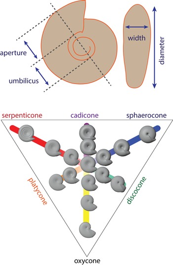
We produced synthetic models of ammonoid conchs in open-source 3D modeling software (Blender v. 2.79c; Unreal v. 4.22) by altering a torus spiral to fit geometric coiling parameters, following Ritterbush and Bottjer (Reference Ritterbush and Bottjer2012): thickness ratio (Th), whorl expansion (w), and umbilical exposure (U) (see Fig. 2). We prepared the models for integration with the fluid simulation software by smoothing them and removing internal features in Zbrush (v. 2019.1.2). We follow the protocol of Jacobs (Reference Jacobs1992) and add a simple conical body extension to each shell, limited to 1 cm length (20% of shell diameter) from the aperture as a conservative estimate of a tucked body like Nautilus. Emulations of Jacobs's shells were fit with soft-body approximations to match his published images (Jacobs Reference Jacobs1992). Physical models were 3D-printed in medical resin at the University of Utah Hospital library, with the aperture oriented at 30° and a teardrop-shaped shaft rising from the center of the shell to anchor it to a force transducer (Fig. 3). Simulations also used the 30° orientation for consistency across the dataset. We employ this aperture angle to provide consistency across all simulations, to remove a variable of iteration to simplify the study, and to provide a baseline from which additional studies might vary. We choose the 30° aperture angle as the midrange of Chamberlain's (Reference Chamberlain1976) experimental settings; to align with Jacobs's (Reference Jacobs1992) settings; and as a midrange value for the aiming of the imagined hyponome (midway between vertical and perpendicular to the shell coiling axis). This choice makes our data applicable to the broadest range of prior experiments while maintaining the dataset as a unified whole that can be directly repeated, used, or discussed in future investigations.
Gross shape of a planispiral ammonoid conch can be represented through three ratios of measurements on a figured specimen: whorl expansion (increase in aperture height over 180° of shell accretion); umbilical exposure (ratio of umbilical diameter to whole conch diameter); and thickness ratio (ratio of conch width to diameter). Each trait is exemplified by oxycone, sphaerocone, and serpenticone morphotypes, respectively (see Ritterbush and Bottjer Reference Ritterbush and Bottjer2012).

Schematic for physical experiments.

Physical Measurements of Drag
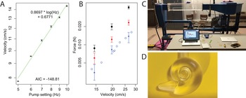
We measured the drag force that moving water exerted on different shell shapes (sphaerocone, oxycone, morphospace center, serpenticone) by attaching models to a force transducer mounted above a flow chamber (100 × 15 × 15 cm) on a flume tank (Fig. 3). Models were attached to the force transducer at a 90° angle on a shaft with a teardrop-shaped cross section and length of ~7 cm to suspend them in the center of flow 20 cm from the inlet and 80 cm from the outlet. Once attached and stabilized, the force transducer was reset to read at zero, and force in the direction of water flow was recorded at 20 Hz. Stream flow speeds were calibrated using a pygmy meter over 5 iterations at each target speed, then were controlled by setting the rotation rate on the flume's water pump. The orthogonal force transducer measurement offers ±0.002 N accuracy, which limits its functional measurement range to a minimum of 2000 dyne. We set test fluid flow velocities between 10 and 25 cm/s for each conch model. Speeds of 10, 15, 20, and 25 cm/s represent the moderate to upper end of previous experiments (i.e., Chamberlain Reference Chamberlain1976; Jacobs Reference Jacobs1992), while fitting within the signal capacity of the force transducer. Each model was (1) placed in quiet water, (2) given a 5-min rest period after setting the transducer to zero, then (3) subjected to three 90 s durations at each target speed in sequence. We turned the pump control to 0 Hz for 30 s between each velocity test, providing a rapid fluid acceleration at the start of each velocity test interval (rather than a monotonic stepwise increase in velocity). Forces were recorded continuously via a cable from the force transducer to a benchtop notebook computer (Fig. 3). From these data, we observed the magnitude of drag force change between 0 Hz and the test velocity, providing three replicates per velocity, per model, during each experimental run. We repeated this protocol in its entirety seven times, providing 21 total replicates per model-velocity test case. Water temperature varied dramatically from the source depending on the day and time of day and warmed throughout flume operation after running through the pump cycle. Instead of factoring temperature into our analyses as an additional variable, we calculated the mean and standard deviation of the least-noisy velocity tests for each model (thus including a broad range of temperatures, without accounting for the role of temperature in this variance). This experimental design and analysis represent an order-of-magnitude benchmark to compare the rank of different conch performances on the target models, rather than a comprehensive assessment rivaling past work (i.e., Chamberlain Reference Chamberlain1976; Jacobs Reference Jacobs1992).
Numerical Simulation of Drag
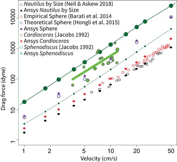
We created a digital water flow simulation using ANSYS FLUENT (v. 18) as a standard space in which to place each ammonoid conch model. The test space was a rectangular prism with dimensions 182.5 cm long, 105 cm wide, and 105 cm deep. In each case, the digital ammonoid model (rendered at a 5 cm conch diameter) was positioned 30 cm from the inlet, according to methods established by Hebdon et al. (Reference Hebdon, Ritterbush and Choi2020b). Figure 4 compares simulation values from Hebdon et al. (Reference Hebdon, Ritterbush and Choi2020b) to published experiments as a demonstration of the first-order efficacy of the method. Prism space surrounding the shell models was discretized into approximately 1 million elements for flow calculations. Wall effects, turbulence models, and mesh settings follow best practices from Hebdon et al. (Reference Hebdon, Ritterbush and Choi2020b) and are shown in Table 1. We initiated each simulation with a fluid inlet velocity ranging from 1 cm/s to 50 cm/s, and each drag estimate was refined by the software until simulation residuals were stable below 1e−3.
Comparison between computational fluid dynamics methods (see text) and published benchmarks for water-tank experiments using both live (Nautilus) and replica (ammonoids Oppelia, Sphenodiscus) specimens. Live Nautilus data are taken from Neil and Askew (Reference Neil and Askew2018; for consistency, showing only drag for animals swimming posteriorly with a type 1 jet at a low angle). Experimental ammonoid replica data are taken from Jacobs (Reference Jacobs1992). See Hebdon et al. (Reference Hebdon, Ritterbush and Choi2020b) for method details. Values for a sphere follow Barati et al. (Reference Barati, Neyshabouri and Ahmadi2014) and Yang et al. (Reference Yang, Fan, Liu and Dong2015).

Computational fluid dynamics settings.

Analysis of Drag
New experiments and simulations were organized to verify, or reject, the basic rank-order of drag forces on the different conch shapes, following interpretations of results from Jacobs (Reference Jacobs1992) and Chamberlain (Reference Chamberlain1976) (Ritterbush Reference Ritterbush2015; see also Seki et al. [Reference Seki, Tanabe, Landman and Jacobs2000], though we eschew the slightly heteromorphic forms in this work for simplicity). Comparing drag forces estimated from different methods (here: experiments, CFD simulation), differently sized models (i.e., Chamberlain Reference Chamberlain1976; Jacobs Reference Jacobs1992; this study), and different velocities of fluid flow requires simplified index values. First, we consider an index to compare drag forces. Coefficient of drag is a dimensionless empirical value, which attempts to isolate the influence of shape on drag force, after accounting for size and velocity. Specifically,
 $${\rm Drag\ force} = 0.5 \times {\rm C}_{\rm d} \times A \times {\rm \rho} \times U^2$$
where U is velocity, ρ is density of the fluid, and A is area to account for size. Size of an ammonoid can here be assessed as a cross section, a surface area, or approximation from volume (volume2/3; i.e., Jacobs Reference Jacobs1992). Our analyses represent size from the model surface area. In short, Cd represents shape contribution to drag.
Next, we must consider the flow behavior inherent to any hydrodynamic test: will fluid flow be smooth or rough? Re is a dimensionless value that contrasts initial force and viscous force. Generally, Re can be used to track transitions between laminar (Stokes flow, very low Re), normal (Newtonian flow, moderate Re), and turbulent flow (breakaway flow, high Re) (Barati et al. Reference Barati, Neyshabouri and Ahmadi2014; Yang et al. Reference Yang, Fan, Liu and Dong2015). As with Cd (eq. 1), calculation of Re acknowledges both velocity and size.
 $${\rm Re\ } = l \times U/k_{\rm v}$$
where k v is kinematic viscosity; U is velocity; and l is a characteristic length to account for size. Throughout this work we set density at 1.027 g/cm3 and kinematic viscosity at 0.01 m2/s. Kinematic viscosity (k v) and density (ρ) can both vary in seawater, so in the discussion we present a simple fan diagram to compare these interactions. In equation (2), length is a single-dimensional value included to estimate size contribution to flow regime. Essentially, Re controls how Cd values are compared: one must correctly assess the system of experimentation (or simulation) to compare the results. We have options concerning how to measure the size component of Re. When Re is standardized to describe fluid motion through a closed system (i.e., a pipe), the size of the chamber is factored in as a characteristic linear measure. Typically, this places Newtonian flow between Re values of 100 and 10,000. Our analyses, however, choose a different framework to represent size.
To assess the flow regime from the perspective of the ammonoid animal, we calculate Re with a geometric approach. To consider flow interaction with the ammonoid, we assess size in relationship to the modeled conch (rather than the chamber itself). This is consistent with Jacobs's (Reference Jacobs1992) use of ammonoid model length-in-flow as the characteristic length in Re calculations (which we also employed in Hebdon et al. Reference Hebdon, Ritterbush and Choi2020b). Here, we linearize volume (volume1/3) as the characteristic length in equation (2). This serves two direct purposes. First, linearized volume presents a more generalized assessment of a conch's potential interruption of, or interaction with, flow. Second, framing all experiments and simulations around the volume of the test subject allows us to directly compare Cd results across the full range of Re.
These refined Cd and Re values allow us to compare our results with those of previous work. Generally, drag caused by shape alone will decrease as the object's size and/or speed increases, because viscous drag acting along the whole surface is proportionally lower relative to the whole pressure drag acting on the cross-sectional, or frontal, area (Barati et al. Reference Barati, Neyshabouri and Ahmadi2014; Yang et al. Reference Yang, Fan, Liu and Dong2015). For each conch model, we fit simple functions to describe changes in Cd with increasing Re. We also view the relative contributions of viscous and pressure drag coefficients as a function of the increase in Re.
Growth Assessments
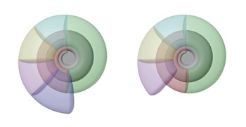
We modeled a series of basic ammonoid shapes, then removed a slice of newest-accreted shell from the aperture end of the final whorl (Fig. 5). This portion of removed shell can represent an aliquot of biomineralized material. Using this biomineralized material as a currency, we measure how each morphotype changes volume, surface area, diameter, and venter length (similar to circumference) per unit of added material.
Ammonoid conch models as tested (left; sans soft-body extension), and with one aliquot of external shell biomineralization removed (right). Septa are ignored. (“Cap” on aperture is shown for clarity, excluded from measurements.)

Models of Ammonoid Shell Motion
Data published for Nautilus (Neil and Askew Reference Neil and Askew2018) show that the motion across a single mantle contraction differs from the animal's corresponding mantle extension. In contrast, our methods approximate the drag force from a stable, constant flow of fluid at a fixed velocity. To interpret our results in the context of an ammonoid swimming against the resistance of its shell, we calculate a “compensation velocity.” Jet propulsion generates punctuated motion, causing complex relationships between energy expense and forward motion (see recent demonstrations with live Nautilus [Neil and Askew Reference Neil and Askew2018] and squid [Bartol et al. Reference Bartol, Krueger, Jastrebsky, Williams and Thompson2016]). Here we simplify the problem to postulate a single jet over a single second, with the animal starting at a velocity of zero. For each shell model, we determine the maximum acceleration at which forward force from swimming will be greater than or equal to the negative force from drag. This is a dynamic problem, because both factors change with acceleration. Thus, we solve the problem to a reasonable resolution with a numerical solution in the open-source statistical language R (R Core Development Team 2020). From this, we report the maximum acceleration, maximum velocity, maximum power, and, finally, maximum distance traveled in a single second. Note that this approach deliberately does not address added mass (impacts from vortex formation in the umbilicus and wake as the animal moves) or aspects of the soft tissues (musculature, jet rhythm, etc.). Our only goal is to estimate the challenge produced by the conch itself.
Results
Drag Measurements
Flume measurements are shown in Figure 6. As expected, a moderate sphaerocone generates more drag than a moderate serpenticone, and both shells generate drag consistent with expectations from previous experiments (Jacobs Reference Jacobs1992; Neil and Askew Reference Neil and Askew2018). The force transducer has an accuracy of ±0.002 N, or 200 dyne, which makes measurements at velocities below 10 cm/s impractical.
Experimental results for flume tank experiments with 3D-printed ammonoid shells. A, Velocity calibration on equipment. See text. B, Drag force measurements for each of three models: sphere (black dots), sphaerocone shell (red squares), and serpenticone shell (blue triangles). Each point shows the mean value with bars showing the standard deviation. Open blue circles are data from Jacobs's experiments with a cast of the serpenticonic Lytoceras (Jacobs Reference Jacobs1992). C, Flume channel at the University of Utah College of Engineering (water chamber is transparent acrylic). D, Experimental model of an idealized serpenticone shell printed in medical resin at the University of Utah Hospital Libraries.

Measurements of Drag and Calculations of Drag Coefficients
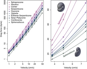
Simulated drag values are shown in Figure 7, and coefficent of drag (Cd) and Reynolds number (Re) are shown in Figure 8. Coefficient of drag (Cd) generally decreases with higher Reynolds number (Re), but different ammonoid shell shapes present substantial variation in the magnitude of this decrease. Generally, decrease of Cd with Re is well represented by a simple exponential decay.
 $${\rm C_d}\sim a \times {\rm Re^{{-}1}} + b$$
Drag measurements from water flow simulated around ammonoid shell models. Left, Full range of values, axes in log scale. Right, Focus on velocities of one shell diameter per second (all included models are 5-cm-diameter shells) for the same range of shapes, with axes in linear scale.

Comparison of drag coefficients with Re for a range of ammonoid shell shapes. Lines between data points are for ease of viewing and do not represent calculated functions.

A polynomial function (eq. 4) provides greater fit.
 $${{\rm C_d}\sim \;a \times {\rm Re^{{-}1}} + b + c \times {\rm log( {Re} )} + d \times {\rm Re}$$
Variation in overall drag relates to underlying trends in both viscous and pressure drag. Figure 9 shows results for three shells. The coefficient of viscous drag decreases continuously, as water gains turbidity and breaks away from friction with the shell surface. Pressure drag, however, relates more to the flow resistance presented by the cross-sectional area of an object, and the coefficient of pressure drag remains stable over orders of magnitude of turbulent Re. Figure 9 also shows the exponential and polynomial fits to the viscous and pressure drag components. These fits allow us to estimate the Cd of each model within a constant Re. Figure 10 compares conch shape and estimated Cd at two fixed Re values.
Trends in coefficients of drag for three shell shapes: sphaerocone (top), serpenticone (center), and oxycone (bottom). Each plot shows the coefficient for overall drag (open circles), as well as coefficients for pressure drag (dots) and viscous drag (squares). Light-colored lines represent a simple exponential decay fit to the data (eq. 3), and dark lines represent a polynomial fit (eq. 4). Gray shaded region marks the Re for which friction drag is greater than pressure drag.

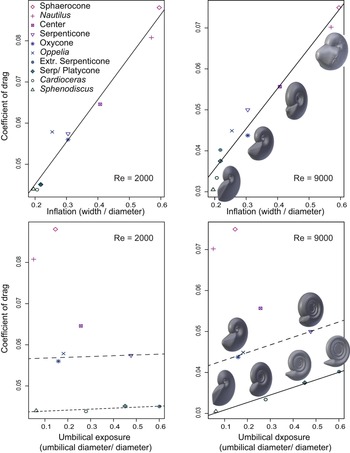
Comparison of coefficient of drag (Cd) with parameters of shell shape. Top row, Cd increases for inflated shells. Bottom row, Increases of Cd with greater umbilical exposure is only clear at higher Re. At Re = 9000, Cd relates to both inflation and umbilical exposure. Dashed lines are not significant and are shown for easy comparison between plots.

Velocity and Power
Maximum velocities for ammonoid swimming speed are estimated at two to three times the shell diameter per second. Compensation velocity is the speed at which the force of the accelerated ammonite, at 1 s, is equal to the opposing force of drag on the shell. Maximum swimming velocity can also be estimated by invoking an effective power per gram of animal soft tissue. Here we apply the 660 erg/g estimate from Jacobs (Reference Jacobs1992) to body-tissue estimates modeled after the observations of Nautilus from Ward et al. (Reference Ward, Stone, Westermann and Martin1977). Figure 11 shows a logistic regression of body mass from total animal mass from 26 specimens of Nautilus reported by Ward et al. (Reference Ward, Stone, Westermann and Martin1977). The nonlinear least squares function in R (R core development team) fit the data to equation (5).
 $$\log ( {\rm mass_{body}} ) = -2.676 + 1.370\;\times \;{\rm log}( {{\rm mas}{\rm s}_{{\rm total}}} ) $$
Total mass (including shell) and body mass (soft tissues) of 26 specimens of Nautilus pompillis, from measurements in Ward et al. (Reference Ward, Stone, Westermann and Martin1977) (note log scale on both axes). The line represents a fit to log-log regression (see text).

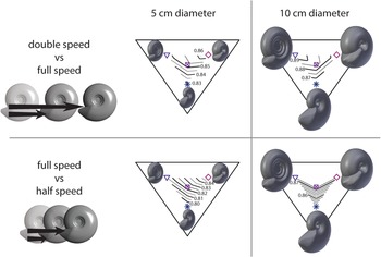
We applied this function to estimate the body mass of each specimen: total mass is volume of each 3D ammonoid model, multiplied by seawater density (1.027 g/ml). At a diameter of 5 cm, each shell presents a similar compensation velocity, but pronounced differences emerge at larger shell sizes. At diameters of 10 cm and above, serpenticonic shells produce the lowest compensation velocity (Fig. 12A). The equal-power approach produces higher potential velocities for the inflated sphaerocone due to its greater volume at a given diameter. The serpenticone conch still produces the lower range of velocity above diameters of 15 cm. Values for both velocity estimates are presented for shells of 5 and 10 cm diameters in Table 2. Figure 13 shows only four key morphotypes for ease of comparison. Another comparison of shell hydrodynamic efficiency is the power required to push the shell at a higher velocity. We calculated the power required to overcome drag force while traveling one half-diameter per second, one diameter per second, or two diameters per second. The increase in power required for each step is shown as a power of 10 in Figure 12. At small sizes, the power increase is more severe for the inflated sphaerocone shell, but above 10 cm diameter, the serpenticone shell shows the greatest increase in power required to go a single diameter per second (Fig. 12C). To move two diameters per second, the serpenticone shell is less efficient at diameters above 7 cm (Fig. 12D).
Potential ranges of swimming velocity and power requirements for four idealized ammonoid shell shapes, across a range of shell diameters. A, Velocity at which the force from acceleration of the ammonite (after 1 s) would match the opposing drag force on the shell. This compensation velocity ignores added mass. B, Estimated maximum velocity attainable if each animal exerted 400 ergs of power per gram of soft tissue (see text). C, Contrast in power required for the ammonite to combat drag forces at one shell diameter per second vs. power required at one-half shell diameter per second. D, Contrast in power required to overcome drag at two diameters per second vs. one diameter per second.

Interactions between gross conch morphology and power trade-offs in generalized ammonoids. The top panel visualizes results from Fig. 12D. The illustration contrasts an ammonoid moving 2× diameter per second vs. the same animal moving only 1× diameter per second. Top center, Isopachs in Westermann morphospace contour the increased power required for an ammonoid of 5-cm-diameter conch to double velocity from 5 cm/s to 10 cm/s. (Values written in log base 10, as in Fig. 12D: a value of 1 would denote 10× power demand to double velocity.) Top right, An ammonoid of 10-cm-conch diameter, doubling velocity from 10 cm/s to 20 cm/s. The bottom panel visualizes results from Fig. 12C. Bottom left, Consider the ammonoid increasing from one-half a diameter per second to one diameter per second. Bottom center, Increased power demand of an ammonoid with a 5-cm-diameter conch going 5 cm/s instead of 2.5 cm/s. Bottom right, Increased power demand of an ammonoid with a 10-cm-diameter conch going 10 cm/s instead of 5 cm/s.

Velocity estimates for ammonoids with shell diameters of 10 cm.

Growth Assessments
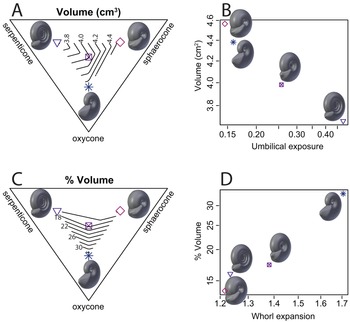
The first-order growth assessments consider only the trends associated with adult shell growth, not growth from the juvenile stage. Each of the three end-member shell shapes of Westermann morphospace emphasize a particular growth characteristic. Results are shown as a heat map in Figure 14, and growth characteristics are compared to conch shape in Figures 15 and 16. For a given budget of surface area (to represent biomineralization effort) sphaerocones produce the most volume of newly added body chamber (in keeping with the greater volume to surface area ratio of spheres in general, and sphaerocones specifically, as in Tendler et al. (Reference Tendler, Mayo and Alon2015). For the same surface area budget, oxycones produce the greatest addition to the whole-shell diameter. Serpenticones, finally, produce the greatest addition of body chamber perimeter measured along the venter.
Heat map tables compare growth aspects of four idealized shell shapes. The top table compares aspects of growth during each shell's most recent 10 cm2 of added shell surface (see text). Each column represents a single aspect of growth (venter length, diameter, etc.), and the highest values are marked with the lightest shading. Compared with the other shells, the serpenticone shows the least gain in diameter, but the greatest gain in venter length. The lower graph shows the percent of shell growth that was attained during the last application of 10 cm2 of surface area. The serpenticone gained 3.34 cm of ventral length during its recent growth, which is over 20% of its ventral margin; both the absolute value and the relative value are greater than that shown for the other shapes. SA, surface area.

Comparison of growth values (Fig. 14) and morphospace parameters. All growth values are normalized to the most recent application of 10 cm2 of outer shell surface (see text). A, Four shells are compared in Westermann morphospace. Diameter gain is greatest for the oxycone shell. B, Diameter gain is associated with the coupled increase of whorl expansion and decrease in inflation (both axes in log scale). C, Venter length gain compared in Westermann morphospace. D, Venter length gain is associated with a coupled increase in umbilical exposure and decrease in inflation (both axes in log scale).

Comparison of volume increase across Westermann morphospace. A, The serpenticone model showed the lowest increase in volume. B, Volume increase has a negative association with umbilical exposure (both axes in log scale). C, Relative volume increase was greatest in the oxycone model. D, Relative volume increase is positively associated with whorl expansion (both axes in log scale).

Discussion
Simulated drag measurements reported here uphold some expectations based on previous work and considerably refine our understanding of the ranking, and orders of magnitude, of hydrodynamic efficiency of different conch shape attributes. As anticipated (Jacobs Reference Jacobs1992; Ritterbush Reference Ritterbush2015; Hebdon et al. Reference Hebdon, Ritterbush and Choi2020a), shells with greater inflation typically cause higher drag, and have greater Cd for a given Re. Among compressed shells, the umbilical exposure on serpenticones leads to greater drag overall (compared with an oxycone), though this appears to be most influential at larger sizes and/or higher speeds. The results yield new insight on the dynamic drag states of serpenticonic shells. Among the shapes examined, small serpenticone conchs may accommodate the fastest acceleration, but at the cost of very low efficiency (contrast possible velocity shown in Fig. 12A, compared with the power required to achieve that velocity shown in Fig. 12C). Larger serpenticone conchs could probably not reach such high velocities in terms of shell lengths per second, but may have afforded relatively moderate efficiency (Fig. 12B,C). The results invite speculation on ammonoid paleoecology, some aspects of which can be tested through further analyses.
We present first-order estimates of the compensation velocity for each shell shape: the speed at which forward force would match drag force, ignoring added mass. These calculations demonstrate how drag on the shell presents different challenges to different ammonoid animals, depending on their sizes and velocities. For now, we ignore added mass on the shell for two reasons. First, soft-tissue behavior is a second-order influence on whole-body drag, but may prevent, shed, or collect added mass during a single jet. Rather than assessing the soft-tissue mitigation of added mass in our minimalistic fixed-shape 3D ammonite models, we anticipate that relevant results will continue to emerge from ongoing biomechanics experiments on living cephalopods.
Emerging techniques to observe and measure fluid dynamics in live-animal experiments and simulations are transforming biomechanical concepts of swimming efficiency in cephalopods. New work presents greater attention to pressure zones (Dabiri et al. Reference Dabiri, Bose, Gemmell, Colin and Costello2014; Gemmell et al. Reference Gemmell, Colin, Costello and Dabiri2015), wakes and eddies (Peng and Dabiri Reference Peng and Dabiri2008), and spiral vortices (Bartol et al. Reference Bartol, Krueger, Jastrebsky, Williams and Thompson2016; Neil and Askew Reference Neil and Askew2018; Xiang et al. Reference Xiang, Qin and Liu2018). Cephalopod jet propulsion, long regarded as woefully inefficient (e.g., Wells Reference Wells1990; O'Dor Reference O'Dor2002), is now shown to induce vortex fields that increase efficiency at increasing velocity for both squid (Lolliguncula brevis; Bartol et al. Reference Bartol, Krueger, Jastrebsky, Williams and Thompson2016) and Nautilus (Neil and Askew Reference Neil and Askew2018). For squid, vortex dynamics make jet propulsion even more efficient than fin swimming (Bartol et al. Reference Bartol, Krueger, Jastrebsky, Williams and Thompson2016), overturning a long-standing paradigm. New experiments with live Nautilus (Neil and Askew Reference Neil and Askew2018) demonstrated two efficient modes of transportation: slow anterior swimming (arms first, 0.5 body length/s), or fast posterior swimming (shell first, 1.5 body lengths/s). Jet propulsion can generate distinct or elongated vortices (Neil and Askew Reference Neil and Askew2018). In squid, Bartol et al. (Reference Bartol, Krueger, Jastrebsky, Williams and Thompson2016) observed positive associations between velocity, jet period, vortex elongation, and efficiency across both swimming orientations. In contrast, Neil and Askew (Reference Neil and Askew2018) show that faster Nautilus used shorter jet periods, particularly in the posterior-first direction. Nautilus achieved their highest thrust with elongated jet vortices but did not clearly favor this mode in either swimming orientation. Vortex structures may relate to maneuverability, in which case one must consider the experimental designs in these very different studies: squid traveling along a flow channel versus Nautilus pursuing an offered shrimp around a cuboid aquarium.
These recent experiments show that living animals’ behavior can mitigate the innate challenges of their body plan, but that this body plan still drives the order of magnitude differences in their motility costs, range of reasonable swimming speeds, and metabolic demands. Nautilus apparently spend most of their time traveling slowly and efficiently, and move quickly with brief, rapid jets at the expense of some efficiency (Neil and Askew Reference Neil and Askew2018). Interestingly, preliminary results show opposite effects in squids and Nautilus. Bartol et al. (Reference Bartol, Krueger, Jastrebsky, Williams and Thompson2016) observed positive associations between squid speed, jet period, and efficiency across both swimming orientations. Neil and Askew (Reference Neil and Askew2018) observed a tiered system, with the most efficient travel as long-period jets in slow anterior-first locomotion and the most powerful thrust coming from short-jet posterior-first locomotion. This final case matches the behavior we are modeling for ammonoids. Here we quantify challenges presented by the ammonoid conch shape as a foundation for future work to assess the selective pressures and mitigating innovations at play in ammonoid evolution. Crucial, too, all ammonoids were born as small hatchlings, and many changed their overall conch form throughout ontogeny. Indeed, trends in conch shape through ontogeny are one of the primary features illustrated by Westermann in the 1996 diagram that inspired a quantification of Westermann morphospace. Thus, any large-sized ammonoid needed first to survive as a small-sized ammonoid and may have done so using a very different conch morphology.
Our first-order compensation velocity results present the possibility that small serpenticone ammonoids had the potential to move farther in a single second than ammonoids with different shell shapes, but at a high cost (requiring a hefty jet action). We speculate that this degree of maximum motion would be used only rarely, as an escape from a predator, and for a very limited duration. For even casual locomotion, the cost of propulsion for serpenticones is higher than for more streamlined shells, so these animals probably did not move swiftly very often. Based on this, we further speculate that these animals might have had fairly low baseline metabolic rates. An ammonoid with an oxycone shell, in contrast, would require far less energy to propel at a maximum acceleration each second. Moving forward, these interpretations must be subject to further scrutiny. One tactic is to estimate the power that an ammonoid could generate from within a serpenticonic shell. Jacobs (Reference Jacobs1992) took the approach of estimating the power an animal in each shell shape could generate, then calculating the velocity that it could reach. Newer 3D models allow estimation of ammonoid soft-tissue distribution and potential water jet chamber volume with greater nuance. Calculations of the potential power generated within the body chambers of ammonoid shells should help to constrain whether the animals could take advantage of shell shapes that would withstand greater accelerations. Dramatic advances in recognizing ammonoid soft-body form (i.e., Klug et al. Reference Klug, Schweigert, Tischlinger and Pochmann2021) are likely to revise estimations of their range of muscle and jet capacity.
Trade-offs between maximum acceleration and energy requirement differ when conch size is increased. Large serpenticone conchs would allow the lowest acceleration and would move the shortest distance during a single second compared with other conch shapes. Our broad interpretation of this result is simply that large serpenticonic shells did not provide advantages for rapid locomotion. When these shells appear in the fossil record, we favor ecological and evolutionary interpretations that do not invoke a selective pressure for rapid swimming in these species at sizes greater than ~5 cm. In the specific case of the Early Jurassic diversification of ammonoids after the end-Triassic mass extinction, we speculate that large serpenticone species (i.e., Psiloceras pacificum, Psiloceras polymorphum, Arietites lyra) could have sized out of predation pressure from species with smaller, more efficient shells, for example, the moderate platycone of Nevadaphyllites compressus. Only a very small percentage of an ammonoid reproductive cohort should be expected to have reached these great sizes, and most may have fallen prey to conspecific predation (e.g., Bucher et al. Reference Bucher, Landman, Klofak, Guex, Landman, Tanabe and Davis1996; Kerr and Kelley Reference Kerr and Kelley2015; Klug et al. Reference Klug, Baets, Kröger, Bell, Korn and Payne2015). In this scenario, ammonoid individuals with very large serpenticonic shells were abundant not because of superior swimming speed or selective pressure favoring that shell shape. In contrast, it appears some individuals survived to large sizes and then faced little selective pressure against this cumbersome shell. Many species of earliest Jurassic ammonites may have been “successful slackers,” gaining abundance, cosmopolitan distribution, and species-level diversity in spite of, not driven by, their sometimes-large serpenticonic shells.
Exterior ornament is also controversial. Spines may have served as defense or may have held a sensory role (Ifrim et al. Reference Ifrim, Bengston and Schweigert2018); in either case, spines would be expected to alter wake dynamics. Ribbing has been interpreted as primarily responding to antipredatory defense escalation (Ward Reference Ward1981; Kerr and Kelley Reference Kerr and Kelley2015) or hydrodynamic streamlining (Chamberlain Reference Chamberlain1980; Lukeneder Reference Lukeneder, Klug, Korn, De Baets, Kruta and Mapes2015). Covariation of rib ornament intensity and coiling parameters occurs in many ammonoid species (De Baets et al. Reference De Baets, Bert, Hoffmann, Monnet, Yacobucci, Klug, Klug, Korn, De Baets, Kruta and Mapes2015; Naglik et al. Reference Naglik, Rikhtegar and Klug2015). The significance of ribs as hydrodynamic mitigation or augmentation will depend first on the challenges introduced by the smooth shell in each morphotype.
This interpretation of ecological structure is speculative and can be tested by further examinations of shell hydrodynamics and size abundance in the fossil record. First, external ribbing ornament became very prominent during the next few million years of the Sinemurian stage (199.3–198 Ma; Franceschi et al. Reference Franceschi, Corso, Cobianchi, Roghi, Penasa, Picotti and Petro2019), and additional flow simulations can determine whether these ribs would increase acceleration, efficiency, breakage resistance, or all of the above. Kerr and Kelley (Reference Kerr and Kelley2015) include Early Jurassic ribbed species as part of the Mesozoic marine revolution, while Moulton et al. (Reference Moulton, Goriely and Chirat2015) present a first-order mechanical framework for the rise of ribbing intensity on serpenticones specifically. The repeated evolution of oxyconic forms, particularly from lineages that previously yielded serpenticonic forms, is a well-recognized trend in ammonoid natural history (Westermann Reference Westermann, Landman, Tanabe and Davis1996; Monnet et al. Reference Monnet, De Baets and Klug2011), including specific cases of umbilical occlusion (Klug and Korn Reference Klug and Korn2002; Bockwinkel et al. Reference Bockwinkel, Becker and Aboussalam2017). Continued focus on morphological and size dynamics in specific ammonoid fossil assemblages or intraspecies variation (i.e., Yacobucci Reference Yacobucci2004; Hammer and Bucher Reference Hammer and Bucher2006; Klug et al. Reference Klug, De Baets and Korn2016) presents test cases to contrast size, form, and abundance: we might expect that oxycone conchs reach larger sizes, while small serpenticonic forms are more abundant. Both forms are compressed, but the trade-offs in their drag profiles are expressed only at larger sizes or higher speeds.
If we speculate that the earliest Jurassic ammonoids, particularly large species, did not have shells selected by intense top-down predation, we must present reasonable alternatives for the ecological structure and selective framework. Tendler et al. (Reference Tendler, Mayo and Alon2015) presented shell features in the context of pareto optimality, wherein each shape represented a compromise between different functionally valuable traits, which can be applied to distinct fossil assemblages (Klug et al. Reference Klug, De Baets and Korn2016). In our simplified growth analyses, each basic conch type excels at producing some aspect of shell geometry: sphaerocones produced the greatest volume; oxycones produced the greatest shell profile diameter, and serpenticones produced the greatest length of whorl extension along the venter. Indeed, advanced analyses of conch growth patterns (Parent et al. Reference Parent, Bejas and Greco2020; Tajika et al. Reference Tajika, Landman, Hoffmann, Lemanis, Morimoto, Ifrim and Klug2020) emphasize the importance of volume as a first-order consequence of, and perhaps important ecological selective pressure for, specific morphotype development and ontogenetic trends. Ammonoids, of course, produce odd shapes throughout history; and juveniles of species with planispirally coiled conchs are no exception (Klug et al. Reference Klug, De Baets and Korn2016). But serpenticone conches produce the least volume per unit of added shell material in our growth calculations, which stands out from the other conch features. Production of a longer venter (relative to other growth patterns) is neither a typical target of measurement nor frequently invoked as a functional advantage, but it may be important in relationship to hydrodynamic trade-offs for serpenticonic conch shapes.
Serpenticones typically have long body chambers (exceeding a 365° whorl; Saunders and Shapiro Reference Saunders and Shapiro1986; Kröger Reference Kröger2002a). A propulsive advantage to this shape seems unlikely; higher-volume conch shapes would be expected to benefit from added musculature and water jet volume. A fecundity advantage is plausible, particularly in large serpenticone ammonites: rather than a wholesale volume increase, the territory allotted to a particular portion of soft tissue (gonad, egg production, etc.) could be lengthened. Increasing the body chamber length would be a possible alternative to decreasing egg size despite maintaining a narrow aperture opening (De Baets et al. Reference De Baets, Bert, Hoffmann, Monnet, Yacobucci, Klug, Klug, Korn, De Baets, Kruta and Mapes2015; Laptikhovsky et al. Reference Laptikhovsky, Nikolaeva and Rogov2018), emphasizing the need to observe more than overall conch size in ammonoids generally (Monnet et al. Reference Monnet, Klug, De Baets, Mapes, Korn, Klug, De Baets and Kruta2015). Two advantages might result: storing reproductive material far from the aperture and little adjustment needed laterally for other soft-tissue systems when the reproductive materials are deployed.
Finally, one possible ecological advantage of enhanced ventral length is relevant to the food web structure and is readily tested on additional fossils. We speculate that serpenticone shells produced longer body chambers but that an animal's body did not fill the chamber, in contrast to the tight fit of a living Nautilus. We speculate that the animal within a serpenticone conch could withdraw its body fully within the chamber, thereby hiding from predators. This interpretation has been presented independently to explain healed sublethal injuries deep in the body chamber of serpenticonic ammonoids (Kröger Reference Kröger2002a,Reference Krögerb). Indeed, Doguzhaeva and Mapes (Reference Doguzhaeva, Mapes, Klug, Korn, De Baets, Kruta and Mapes2015) conclude from muscle attachment scars that ammonoids with long body chambers may have been better suited to a slower life mode. This may not protect the ammonoid from the crushing jaws of some coleoids (e.g., Klompmaker et al. Reference Klompmaker, Waljaard and Fraaije2009; Klug et al. Reference Klug, Schweigert, Tischlinger and Pochmann2021) or vertebrates (very large fish, marine reptiles), but it would be sufficient to avoid direct attack on the soft parts by the jaws or beak of a similarly sized ammonoid (e.g., Kröger Reference Kröger2002a,Reference Krögerb; Keupp Reference Keupp2006; Kerr and Kelley Reference Kerr and Kelley2015). The interpretation would predict that ammonoids in serpenticone shells could survive attacks that broke substantial portions of the aperture or body chamber, by the animal withdrawing inside and repairing the shell later with a mantle tissue that could extend far back and forth within the body chamber (as in Kröger Reference Kröger2002a,Reference Krögerb). Particular hypotheses might be drawn for soft-body behaviors, to be tested against detailed fossil observations (muscle attachment scars, healed shell from sublethal injures, etc.). Hydrostatic stability and orientation are very sensitive to distribution of the soft body relative to the center of buoyancy (Kröger Reference Kröger2002b; Peterman et al. Reference Peterman, Mikami and Inoue2020b,Reference Peterman, Mikami and Inouec). Retracting the body would certainly have hydrostatic consequences that might intensify how ill-suited these animals would be for continuous swimming. And last, Early Jurassic species with serpenticone conch shapes flourished in the first global takeover by Ammonitina. Their iconic suture complexity may have aided hydrostatic adjustments (Peterman et al. Reference Peterman, Ritterbush, Ciampaglio, Johnson, Inoue, Mikami and Linn2021) to compensate for, or ultimately enable, widespread success as low-metabolism, high-fecundity, risk-avoidant animals.
Conclusions
We present hydrodynamic flow analyses, growth features, and apparent maximum acceleration values for a variety of common ammonoid shell shapes. The maximum acceleration calculations consider only the top rate at which the shells can move to balance their forward and drag forces. These accelerations were not necessarily achieved and could be limited by the animals’ soft body components: muscular distribution, propulsive water volume, and metabolic rate. Indeed, the high power requirements of small serpenticones may suggest that the animals only rarely used such top accelerations, if at all. The acceleration values show trade-offs with size in serpenticone shells, where the top acceleration speeds are limited to the smaller specimens. We speculate on predator–prey dynamics among earliest Jurassic Hettangian ammonoids as an example of how these new data can be brought to bear on specific ecological contexts: we suggest that small specimens of Psiloceras could dodge more streamlined predatory Nevadaphyllites in an emergency, but that the larger specimens effectively sized out of predation by most ammonoids. Postextinction ammonoid shell shape in the earliest Jurassic is unlikely to have been shaped by selective pressures favoring the fastest locomotion across ammonoids generally.
Acknowledgments
This work is dedicated to J. Guex and D. Taylor for their work on Hettangian and Sinemurian ammonoids of North America. We thank S. Naleway and M. Metzger for assistance with equipment and helpful discussions. We thank D. Trentman and C. Cazedessus for tireless computing support. Y. Choi and D. Peterman provided helpful edits to the text. We thank the editor and reviewers, including C. Klug and K. De Baets, for greatly improving the quality of the article. This work is supported by NSF 1945597.
Data Availability Statement
Data available from the Zenodo Digital Repository: https://doi.org/10.5281/zenodo.6368967.