


1. Introduction
The proper design of marine structures is well known to require detailed knowledge about the surface elevation of the surrounding waves. Since real ocean waves are inherently irregular and random due to their spread in frequency, direction and phase, they are most adequately described statistically, and for that reason the probability distributions of the surface and crest elevations have recently attracted considerable attention. For example, Onorato et al. (Reference Onorato, Cavaleri, Fouques, Gramstad, Janssen, Monbaliu, Osborne, Pakozdi, Serio and Stansberg2009), Toffoli et al. (Reference Toffoli, Gramstad, Truelsen, Monbaliu, Bitner-Gregersen and Onorato2010) and Xiao et al. (Reference Xiao, Liu, Wu and Yue2013) have studied these distributions, and their work has, among other things, led to the conclusion that the probability of finding large surface and crest elevations decreases with the directional spread of the wave field. From an engineering point of view, the surface elevation is, however, not the only interesting quantity, as the loads on the structures are ultimately determined by the fluid kinematics that accompany the waves. Despite the great practical importance of the distributions of the fluid velocities and accelerations, contributions to the literature on these aspects have been relatively rare within the last 20 years. On the theoretical side, Song & Wu (Reference Song and Wu2000) have derived the probability density function (PDF) of the fluid velocity at arbitrary depth to second order in wave steepness. Numerical simulations have been carried out by Toffoli et al. (Reference Toffoli, Bitner-Gregersen, Suslov and Onorato2012), who showed that the PDF of the fluid velocity at the surface antiparallel to the surface deviates from that of a normal distribution only for long-crested seas in which modulational instabilities may occur. Other numerical studies have been performed by Sergeeva & Slunyaev (Reference Sergeeva and Slunyaev2013), who investigated whether large fluid velocities at the surface only occur in connection with large surface elevations, and Alberello et al. (Reference Alberello, Chabchoub, Gramstad, Babanin and Toffoli2016), who demonstrated that second-order effects lead to a negative skewness of the PDF of the fluid velocity below the surface. Finally, it has been found from experiments with extreme breaking waves that the velocity and acceleration fields exhibit a substantial degree of front/back asymmetry (Grue & Jensen Reference Grue and Jensen2006) and that the results of common techniques for the estimation of the velocity profile from measurements of the surface elevation may deviate substantially from the actual velocity profiles for certain extreme waves (Alberello et al. Reference Alberello, Chabchoub, Monty, Nelli, Elsnab and Toffoli2018). Although the work mentioned here certainly does not cover all contributions to the kinematics of irregular wave fields, we note that e.g. a systematic study of the dependence of the statistical properties of the fluid velocities and accelerations on the wave steepness has not been carried out until now.
Obtaining exact expressions in closed form for the PDFs of the surface elevation and the fluid kinematics has so far proven an exceedingly difficult task due to the nonlinearity of the governing equations. On the other hand, a number of approximate methods for finding the PDFs exist, and for the surface and crest elevations two rather different approaches seem to prevail. The first of these is the narrowband approach, with which a first-order result was derived by Longuet-Higgins (Reference Longuet-Higgins1952) and a second-order result was found by Tayfun (Reference Tayfun1980). Although its underlying assumptions are, when taken strictly, rarely satisfied, the PDFs found using the narrowband approach are very simple and they require no parameter estimation, as they incorporate the wave steepness explicitly. The second approach is the Gram–Charlier method which was used for the first time in connection with water waves by Longuet-Higgins (Reference Longuet-Higgins1963), and was used to determine the PDF of the crest height one year later by Longuet-Higgins (Reference Longuet-Higgins1964). This approach is, in principle, free of any assumptions about the wave field, and computing the PDF to arbitrarily high order with this method is conceptually straightforward. The method, however, suffers from the fact that it takes the wave steepness into account implicitly through the cumulants of the underlying variable, which may require a substantial amount of data to estimate accurately. In addition, the PDF may become (slightly) negative for sufficiently large negative surface and crest elevations. For both approaches it holds, however, that only their formal accuracy (i.e. the power of the steepness to which the error is proportional) is known a priori, and that a comparison to experimental or numerical results must be carried out in order to establish the actual accuracy for a specific steepness. It appears that the narrowband approach has only been tested thoroughly in the case of weakly nonlinear wave fields, while the Gram–Charlier approach is yet to be thoroughly examined in all cases.
The numerical simulation of large irregular wave fields remains a formidable task on today's computers, even when assuming the wave motion to be described by the potential flow formalism. For that reason, most simulations of irregular wave fields have been performed using either the nonlinear Schrödinger equation and variants hereof (see e.g. Dysthe et al. (Reference Dysthe, Trulsen, Krogstad and Socquet-Juglard2003) and Socquet-Juglard et al. (Reference Socquet-Juglard, Dysthe, Truelsen, Krogstad and Liu2005) as well as the review by Onorato & Suret (Reference Onorato and Suret2016)), the Zakharov equation (see e.g. Annenkov & Shrira Reference Annenkov and Shrira2009, Reference Annenkov and Shrira2013, Reference Annenkov and Shrira2018) or a low-order truncation of the high-order spectral (HOS) method (see e.g. Toffoli et al. Reference Toffoli, Gramstad, Truelsen, Monbaliu, Bitner-Gregersen and Onorato2010; Xiao et al. Reference Xiao, Liu, Wu and Yue2013; Fedele et al. Reference Fedele, Brennan, Ponce de León, Dudley and Dias2016), which are all weakly nonlinear models. While computationally very efficient, their long term accuracy and robustness must be taken with some degree of caution when used to simulate steep wave fields, since e.g. Dommermuth & Yue (Reference Dommermuth and Yue1987) have shown that their implementation of the HOS method could not be used to simulate steady nonlinear waves in deep water steeper than approximately 80 % of the limiting steepness. At the same time, the weakly nonlinear methods do not generally offer the possibility of computing the velocity and acceleration fields below the surface, and simulations based on different numerical methods are therefore necessary, if the distributions of the fluid kinematics are to be determined.
This paper presents an attempt to partially fill the voids described above by studying the statistical properties of both the surface elevation and the fluid kinematics of irregular, directionally spread wave fields in deep water using a fully nonlinear numerical method. Denoting the peak wavelength and period by  $\lambda _p$ and
 $T_p$, respectively, we simulate the time evolution of wave fields of size
 $50 \lambda _p \times 50 \lambda _p$ for times up to
 $100T_p$ using the very recently developed pseudospectral method of Klahn, Madsen & Fuhrman (Reference Klahn, Madsen and Fuhrman2020), which solves the Laplace equation in the entire fluid domain using a stretching of the vertical coordinate while utilizing an artificial boundary condition close to the surface to maintain computational efficiency. The method has been shown to be capable of delivering highly accurate results for challenging wave problems in deep water, and is without doubt substantially more accurate and robust than the above mentioned approximate methods. Moreover, the method has the ability to accurately compute the fluid kinematics throughout the water column even below the steepest (non-breaking) waves. Initializing the simulations from a directional JONSWAP spectrum, we use the method for the time integration of the wave fields, and extract the statistical properties of the surface and crest elevations, the fluid kinematics at the surface as well as the largest fluid velocities and accelerations found in connection with very large crests. In all cases we study the role played by the initial wave steepness
 $\varepsilon _0 = k_p H_{m0}(0)/2$, where
 $k_p = 2{\rm \pi} / \lambda _p$ is the peak wavenumber and
 $H_{m0}(t)$ is the significant wave height at time
 $t$ defined as
 \begin{equation} H_{m0}(t) = 4 \langle \eta(t)^{2} \rangle^{1/2}, \end{equation}
where the angle brackets denote spatial averaging and  $\eta (t)$ denotes the surface elevation at time
 $t$.
The remainder of the paper is structured as follows: in § 2 we give a detailed description of the physical system under considerations and its governing equations, and we briefly describe the numerical method used for the simulations. As our simulations are carried out using artificial damping in order to obtain temporal stability, we discuss the effect of the damping on the total energy and the wave steepness in § 3. In § 4 we present results for the skewness and kurtosis of the surface elevation as well as the PDFs of the surface and crest elevations, and we study the average surface elevation close to large crests. In § 5 we investigate the PDFs of the horizontal fluid velocity and the horizontal and vertical fluid accelerations at the surface, and discuss for which surface elevations large fluid velocities and accelerations at the surface are found. In § 6 we determine the PDFs for the largest horizontal fluid velocity and horizontal and vertical fluid accelerations found in connection with large crests, as well as for the locations at which the largest fluid kinematics occur. Finally, conclusions are drawn in § 7.
2. Physical model, governing equations and numerical methods
We consider the time evolution of an irregular wave field which is spatially periodic in the horizontal  $x$- and
 $y$-directions over distances
 $L_x$ and
 $L_y$, respectively. We assume the water to be infinitely deep and its motion to be inviscid, incompressible and irrotational. Moreover, we assume the surface to be single-valued, and we note that this assumption implies that wave breaking cannot take place in the simulations. We choose the coordinate system such that the
 $(x,y)$-plane coincides with the still water plane, and denote the surface elevation at the point
 $(x,y)$ at time
 $t$ by
 $\eta (x,y,t)$. Under the above assumptions, the motion of the water is governed by the irrotational Euler equations, which we express in terms of the velocity potential,
 $\varPhi$. Denoting the surface potential,
 $\varPhi |_{z = \eta }$, by
 $\varPhi _s$ we follow Zakharov (Reference Zakharov1968) and write the equations as
 \begin{gather} \frac{\partial^{2} \varPhi}{\partial x^{2}} + \frac{\partial^{2} \varPhi}{\partial y^{2}} + \frac{\partial^{2} \varPhi}{\partial z^{2}} = 0 \quad \text{for}\ z < \eta, \end{gather}
 \begin{gather}\left.\frac{\partial \varPhi}{\partial z}\right|_{z \rightarrow - \infty} = 0, \end{gather}
 \begin{gather}\frac{\partial \eta}{\partial t} = \left( 1 + \left( \frac{\partial \eta}{\partial x}\right)^{2} + \left(\frac{\partial \eta}{\partial y}\right)^{2} \right) w_s - \frac{\partial \eta}{\partial x} \frac{\partial \varPhi_s}{\partial x} - \frac{\partial \eta}{\partial y} \frac{\partial \varPhi_s}{\partial y}, \end{gather}
 \begin{gather}\frac{\partial \varPhi_s}{\partial t} = -g \eta - \frac{1}{2} \left(\left(\frac{\partial \varPhi_s}{\partial x} \right)^{2} + \left(\frac{\partial \varPhi_s}{\partial y} \right)^{2} \right) + \frac{1}{2} \left( 1 + \left( \frac{\partial \eta}{\partial x}\right)^{2} + \left(\frac{\partial \eta}{\partial y}\right)^{2} \right) w_s^{2}, \end{gather}
where 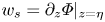 $w_s = \partial _z \varPhi |_{z = \eta }$ is the vertical velocity of the fluid at the free surface and
 $g$ is the gravitational acceleration. This set of equations constitutes an initial value problem for
 $\eta$ and
 $\varPhi _s$, and the remainder of this section is devoted to a description of the initialization of
 $\eta$ and
 $\varPhi _s$, the numerical methods used for the time integration and the computational parameters that we have used.
2.1. Initialization
Given values for the peak wavelength,  $\lambda _p$, and the initial significant wave height,
 $H_{m0}(0)$, we initialize the irregular wave fields from the directional JONSWAP spectrum
 \begin{equation} S(\omega, \theta) = S_0 \left(\frac{\omega}{\omega_p} \right)^{-5} \exp \left( - \frac{5}{4} \left( \frac{\omega}{\omega_p}\right)^{-4} \right) \gamma^{\exp(-(\omega/\omega_p-1)^2/(2\sigma^2))} D(\theta). \end{equation}
Here,  $\omega _p$ is the peak frequency related to the peak wavenumber,
 $k_p$, through the linear dispersion relation for waves in deep water,
 $\omega = (gk)^{1/2}$, the parameter
 $\gamma$ is 3.3 and
 $\sigma = 0.07$ if
 $\omega /\omega _p < 1$ and 0.09 otherwise. Moreover, the directional spreading function
 $D(\theta )$ is chosen to be
 \begin{equation} D(\theta) = \begin{cases} \cos^{2} (\theta) & \text{for}\ | \theta | \le {\rm \pi}/2, \\ 0 & \text{otherwise,} \end{cases} \end{equation}
and the constant  $S_0$ is defined implicitly through the requirement
 \begin{equation} \int_{0}^{2{\rm \pi}} \int_{0}^{\infty} S(\omega, \theta)\,{{\textrm{d}}} \omega\,{{\textrm{d}}} \theta = \left(\frac{H_{m0}(0)}{4} \right)^{2}. \end{equation}
We note that the choice of  $D(\theta )$ gives rise to wave fields which possess a large directional spreading, and for comparison we mention that the wave fields in this work have a larger directional spreading than the wave fields studied by e.g. Onorato et al. (Reference Onorato, Cavaleri, Fouques, Gramstad, Janssen, Monbaliu, Osborne, Pakozdi, Serio and Stansberg2009) and Toffoli et al. (Reference Toffoli, Gramstad, Truelsen, Monbaliu, Bitner-Gregersen and Onorato2010).
Due to the assumed spatial periodicity of the wave field, the numerical method assumes  $\eta$ and
 $\varPhi _s$ to be given by truncated Fourier series, i.e.
 \begin{gather} \eta(x,y,t) = \sum_{n_x = -N_x}^{N_x-1} \sum_{n_y = -N_y}^{N_y-1} \hat{\eta}_{n_x, n_y} \exp \left( \text{i} \boldsymbol{k}_{n_x, n_y} \cdot \boldsymbol{r} \right), \end{gather}
 \begin{gather}\varPhi_s(x,y,t) = \sum_{n_x = -N_x}^{N_x-1} \sum_{n_y = -N_y}^{N_y-1} \hat{\varPhi}_{n_x, n_y} \exp \left(\text{i} \boldsymbol{k}_{n_x, n_y} \cdot \boldsymbol{r} \right), \end{gather}
where  $\boldsymbol {r} = (x,y)$ and
 $\boldsymbol {k}_{n_x, n_y} = (2{\rm \pi} n_x/L_x, 2{\rm \pi} n_y/L_y)$. The initialization of the wave field thus amounts to computing the sets of Fourier coefficients
 $\{\hat {\eta }_{n_x, n_y} \}$ and
 $\{ \hat {\varPhi }_{n_x, n_y} \}$ from (2.2). To do so we follow the two-step procedure outlined by Tanaka (Reference Tanaka2001), in which the frequency
 $\omega _{n_x, n_y}$ is related to
 $\boldsymbol {k}_{n_x, n_y}$ by the linear deep-water dispersion relation
 $\omega _{n_x, n_y}^{2} = g |\boldsymbol {k}_{n_x, n_y}|$. The first step of the method is to compute the so-called complex amplitude
 $b_{n_x, n_y}$ given by
 \begin{equation} b_{n_x, n_y} = \left( \frac{2{\rm \pi}^{2} g^{3}}{ \omega_{n_x, n_y}^{4} L_x L_y} S(\omega_{n_x, n_y},\theta_{n_x, n_y}) \right)^{1/2} \textrm{e}^{\text{i} \phi_{n_x, n_y}}, \end{equation}
in which  $\phi _{n_x, n_y}$ is a random number drawn from a uniform distribution over the interval
 $[0,2{\rm \pi} ]$ and
 $\theta _{n_x, n_y}$ is the angle between the
 $x$-axis and
 $\boldsymbol {k}_{n_x, n_y}$ measured positively counterclockwise. From the complex amplitude,
 $\hat {\eta }_{n_x, n_y}$ and
 $\hat {\varPhi }_{n_x, n_y}$ may then be calculated using the relations
 \begin{equation} \hat{\eta}_{n_x, n_y} = \left( \frac{|\boldsymbol{k}_{n_x, n_y}|}{2 \omega_{n_x, n_y}} \right)^{1/2} \left( b_{n_x, n_y} + b_{-n_x, -n_y}^{\ast}\right), \end{equation}
and
 \begin{equation} \hat{\varPhi}_{n_x, n_y} = - \text{i} \left(\frac{\omega_{n_x, n_y}}{2 |\boldsymbol{k}_{n_x, n_y}|}\right)^{1/2} \left(b_{n_x, n_y} - b_{-n_x, -n_y}^{\ast}\right), \end{equation}
where the symbol  ${}^{\ast }$ denotes complex conjugation.
2.2. Numerical methods
For the time integration of the wave field we use our recently developed pseudospectral volumetric method (Klahn et al. Reference Klahn, Madsen and Fuhrman2020), which may be thought of as consisting of two independent parts. The first part treats the time integration of  $\eta$ and
 $\varPhi _s$ under the assumption that
 $w_s$ is known. The second part deals with the computation of
 $w_s$ from
 $\eta$ and
 $\varPhi _s$ and is inspired by the work of Nicholls (Reference Nicholls2011), as it utilizes the same strategy to reduce the size of the computational domain when solving the Laplace equation (2.1a). In what follows we will briefly describe these two parts, as well as how the method may be used for the computation of the velocity and acceleration fields of the fluid. For a full description and validation of the method we refer to our paper Klahn et al. (Reference Klahn, Madsen and Fuhrman2020).
2.2.1. Time integration
Based on the spatial periodicity of the wave field, the numerical method discretizes the spatial part of (2.1c) and (2.1d) using the Fourier collocation method (see e.g. Kopriva Reference Kopriva2009), in which the equations are satisfied identically at the set of grid points
 \begin{equation} \left\{(x_{n_x}, y_{n_y} ) = \left.\left(\frac{L_x n_x}{2 N_x}, \frac{L_y n_y}{2 N_y} \right)\right| 1 \le n_x \le 2N_x \ \text{and}\ 1 \le n_y \le 2N_y \right\}. \end{equation}
The spatial derivatives of  $\eta$ and
 $\varPhi _s$ at the grid points are calculated from the truncated Fourier series (2.5), and the link between the grid point values and the expansion coefficients is provided by the fast Fourier transform and its inverse. The spatial discretization generates a system of coupled ordinary differential equations describing the time evolution of the grid point values of
 $\eta$ and
 $\varPhi _s$, and we integrate this system in time using the classical fourth-order Runge–Kutta method with fixed step size
 ${\rm \Delta} t$.
When carried out without any kind of energy dissipation, we have found the simulations to be unstable in such a way that they blow up after a after a few peak periods. We note that the unstable behaviour may be provoked by a combination of the facts that the initial condition described above is based on linear theory, and that wave breaking is not allowed in the simulations. As a remedy to the former, we use the adjustment scheme of Dommermuth (Reference Dommermuth2000) in which the nonlinear interactions among the Fourier coefficients of  $\eta$ and
 $\varPhi _s$ are ramped up smoothly on the time scale
 $T_a$. This is done by multiplying the nonlinear terms of (2.1c) and (2.1d) by the function
 \begin{equation} R(t) = 1 - \exp \left( - \left( \frac{t}{T_a}\right)^{n} \right), \end{equation}
where  $n$ is a parameter to be specified. For a precise definition of what is meant by the nonlinear terms in this connection we refer to the paper of Dommermuth. To combat instabilities which arise, because our numerical method does not take wave breaking into account, we follow Xiao et al. (Reference Xiao, Liu, Wu and Yue2013) and multiply the
 $(n_x,n_y)$th Fourier coefficient of
 $\eta$ and
 $\varPhi _s$ by the number
 \begin{equation} D_{n_x, n_y} = \exp \left( - \left( \frac{| \boldsymbol{k}_{n_x, n_y}|}{8 k_p} \right)^{30} \right), \end{equation}
every time step. In this way energy is dissipated from the high end of the wavenumber spectrum, consistent with what is found in laboratory and field experiments (see Xiao et al. (Reference Xiao, Liu, Wu and Yue2013) and references therein). This energy dissipation allows the simulations to be carried out without instabilities, but we stress that it e.g. does not introduce the amplification of fluid velocities occurring in connection with breaking waves (Alberello et al. Reference Alberello, Chabchoub, Monty, Nelli, Elsnab and Toffoli2018). If such effects are to be taken into account, the potential flow formalism used in this work must be abandoned and a numerical method based on the full Navier–Stokes equations must be used.
2.2.2. Computation of  $w_s$ from $\eta$ and $\varPhi _s$


To compute  $w_s$ from
 $\eta$ and
 $\varPhi _s$, one must solve the Laplace problem consisting of (2.1a) and (2.1b) supplemented with the boundary condition
 $\varPhi |_{z = \eta } = \varPhi _s$. To do so, we divide the fluid domain into an upper part with
 $z > -b$ and a lower part with
 $z < -b$, where
 $b$ is a positive number such that the level
 $z = -b$ lies below the lowest trough of the wave field. By solving the Laplace equation analytically on the lower part of the domain, it can be shown (see e.g. § 5 in the paper of Nicholls (Reference Nicholls2011)) that the full Laplace problem is equivalent to solving the reduced problem
 \begin{gather} \frac{\partial^{2} \varPhi}{\partial x^{2}} + \frac{\partial^{2} \varPhi}{\partial y^{2}} + \frac{\partial^{2} \varPhi}{\partial z^{2}} = 0 \quad \text{for}\ -b < z < \eta, \end{gather}
 \begin{gather}\varPhi |_{z = \eta} = \varPhi_s, \end{gather}
 \begin{gather}\frac{\partial \varPhi}{\partial z}(x,y,-b) - T[\varPhi |_{z = -b}] = 0, \end{gather}
on the upper part of the domain. Here, the linear operator  $T$ is defined by the action
 $T[ \textrm {e}^{\textrm {i} \boldsymbol {k}\cdot \boldsymbol {r}}] = |\boldsymbol {k}| \textrm {e}^{\textrm {i} \boldsymbol {k}\cdot \boldsymbol {r}}$ for all
 $\boldsymbol {k}$, and we note that this definition of
 $T$ differs slightly from the definition used in Klahn et al. (Reference Klahn, Madsen and Fuhrman2020) (see (11) in that paper), because we take the water to be infinitely deep in this work. To solve the reduced Laplace problem (2.12) we make the coordinate transformation
 $(x,y,z) \mapsto (x,y,s)$ with
 $s$ defined as
 \begin{equation} s(x,y,z) = \frac{2z + b - \eta(x,y)}{b + \eta(x,y)}, \end{equation}
and define the function  $F$ by
 $F(x,y,s(x,y,z)) = \varPhi (x,y,z)$. From the Laplace equation (2.1a) and the chain rule it then follows that
 $F$ must satisfy the equation
 \begin{align} 0 &= \frac{\partial^{2} F}{\partial x^{2}} + \frac{\partial^{2} F}{\partial y^{2}} + \left(\left(\frac{\partial s}{\partial x}\right)^{2} + \left(\frac{\partial s}{\partial y}\right)^{2} + \left( \frac{\partial s}{\partial z}\right)^{2}\right) \frac{\partial^{2} F}{\partial s^{2}} \nonumber\\ &\quad + 2 \frac{\partial s}{\partial x} \frac{\partial^{2} F}{\partial x \partial s} + 2 \frac{\partial s}{\partial y} \frac{\partial^{2} F}{\partial y \partial s} + \left(\frac{\partial^{2} s}{\partial x^{2}} + \frac{\partial^{2} s}{\partial y^{2}}\right) \frac{\partial F}{\partial s}, \end{align}
as well as the boundary conditions
 \begin{gather} F |_{s = 1} = \varPhi_s, \end{gather}
 \begin{gather}\frac{2}{b + \eta} \frac{\partial F}{\partial s}(x,y,-1) - T[F(x,y,-1)] = 0. \end{gather}
To compute  $F$ numerically, we consider the set of grid points
 \begin{equation} \left\{ (x_{n_x}, y_{n_y}, s_{n_s} )\,|\, 1 \le n_x \le 2N_x,\ 1 \le n_y \le 2N_y \ \text{and}\ 0 \le n_s \le N_s \right\}, \end{equation}
in which  $x_{n_x}$ and
 $y_{n_y}$ are given by (2.9) and
 $s_{n_s}$ is the
 $n_s$th point of the Legendre–Gauss–Lobatto quadrature of order
 $N_s$, ordered such that
 $s_0 = -1$, i.e. from left to right. We moreover assume that
 $F$ is of the form
 \begin{equation} F(x,y,s) = \sum_{n_x = -N_x}^{N_x-1} \sum_{n_y = -N_y}^{N_y-1} \sum_{n_s = 0}^{N_s} \hat{F}_{n_x, n_y, n_s} \exp \left( \text{i} \boldsymbol{k}_{n_x, n_y} \cdot \boldsymbol{r} \right) l_{n_s}(s), \end{equation}
where  $l_{n_s}$ is the
 $n_s$th Lagrange polynomial of order
 $N_s$, and require the boundary conditions (2.15) to be satisfied identically at the points where
 $n_s = N_s$ and
 $n_s = 0$, respectively, and the (2.14) to be satisfied at the remaining
 $4N_x N_y (N_s-1)$ points. We solve the resulting system of linear equations for the values
 $F$ at the grid points using the generalized minimal residual (GMRES) method (Saad & Schultz Reference Saad and Schultz1986) with a preconditioner inspired by the work of Fuhrman & Bingham (Reference Fuhrman and Bingham2004). Finally, we compute
 $w_s$ from
 $F$ using the relation
 \begin{equation} w_s = \frac{\partial s}{\partial z} \left.\frac{\partial F}{\partial s} \right|_{s = 1}, \end{equation}
which follows directly from the definition of  $w_s$ and the chain rule.
2.2.3. Computation of velocity and acceleration fields
By definition of the velocity potential, the velocity field,  $\boldsymbol {v} = (v_x, v_y, v_z)^\textrm {T}$, is given by the relation
 $\boldsymbol {v} = \boldsymbol {\nabla } \varPhi$ where
 $\boldsymbol {\nabla } = (\partial _x, \partial _y, \partial _z)^\textrm {T}$ is the gradient in Cartesian coordinates. From this it follows that we can compute the velocity field as
 $\boldsymbol {v} = \tilde {\boldsymbol {\nabla }} F$ where the operator
 $\tilde {\boldsymbol {\nabla }}$ is defined as
 \begin{equation} \tilde{\boldsymbol{\nabla}} = \boldsymbol{\nabla} + (\boldsymbol{\nabla} s) \frac{\partial}{\partial s}, \end{equation}
and it is understood that  $\partial _z F = 0$. The acceleration field,
 $\boldsymbol {a} = (a_x, a_y, a_z)$, is defined through the relation
 $\boldsymbol {a} = (\partial _t + \boldsymbol {v} \boldsymbol {\cdot } \boldsymbol {\nabla }) \boldsymbol {v}$ and its computations requires somewhat more effort, since the time derivative of the velocity potential,
 $\partial _t \varPhi$, must be known. The function
 $\partial _t \varPhi$ can be shown to satisfy the Laplace problem (2.12) but with the boundary condition (2.12b) replaced by the condition
 $(\partial _t \varPhi ) |_{z = \eta } = \partial _t \varPhi _s - w_s \partial _t \eta$, and
 $\partial _t \varPhi$ can therefore be obtained with the procedure described in § 2.2.2 to obtain
 $\varPhi$. Defining
 $G(x,y,s(x,y,z)) = \partial _t \varPhi (x,y,z)$ at a fixed point in time we thus have
 \begin{equation} \boldsymbol{a} = \tilde{\boldsymbol{\nabla}} G + \left( \left( \tilde{\boldsymbol{\nabla}} F \right) \boldsymbol{\cdot}\tilde{\boldsymbol{\nabla}} \right) \left( \tilde{\boldsymbol{\nabla}} F \right), \end{equation}
which is used to compute the acceleration field.
2.3. Computational parameters and efficiency
In an attempt to add simplicity to the presentation, we have chosen to collect the values of all computational parameters in this section. As basic dimensional parameters of the wave fields we use the gravitational acceleration  $g = 9.81$ m s
 $^{-2}$ and the peak wavelength
 $\lambda _p = 275$ m (corresponding to the peak period
 $T_p = 13.3$ s). We specify a wave field through its initial steepness
 $\varepsilon _0 = k_p H_{m0}(0)/2$, from which the initial significant wave height is trivially computed. Throughout this paper
 $\varepsilon _0$ takes the values
 $0.05$,
 $0.10$,
 $0.15$,
 $0.20$,
 $0.25$,
 $0.30$, and for each value we simulate 20 realizations of the JONSWAP spectrum (2.2). We take the computational domain to have dimensions
 $L_x = L_y = 50\lambda _p$ and discretize it using
 $N_x = N_y = 512$ corresponding to approximately 20 grid points per peak wavelength, since the total number of points in each of the
 $x$- and
 $y$-directions is
 $2N_x = 2N_y = 1024$, respectively. When integrating
 $\eta$ and
 $\varPhi _s$ in time we use the time step
 ${\rm \Delta} t = T_p/50$ corresponding to the Courant number
 $(\lambda _p/T_p ) / ({\rm \Delta} t/ {\rm \Delta} x) \approx 0.4$, and we carry out the time integration for the time interval
 $0 \le t \le 100T_p$. For the adjustment scheme of Dommermuth (Reference Dommermuth2000) we choose the parameters in (2.10) as
 $T_a = 10T_p$ and
 $n = 4$. When solving the reduced Laplace problem (2.12) we choose
 $b = 1.5 H_{m0}$ and take
 $N_s = 10$ such that the upper part of the domain is discretized with 11 points in the vertical direction. We note that if we had not used the artificial boundary condition, but instead worked with a finite water depth,
 $h$, we would have had to require
 $h = O(L_x)$ in order to simulate an infinite water depth, and with the choice
 $b = 1.5H_{m0}$ one finds that this requirement leads to
 $h/b = O(100/\varepsilon _0)$. As such, the artificial boundary condition enables us to work with a computational domain which is between several hundred and several thousand times smaller than the entire fluid domain. The system of linear equations resulting from the reduced Laplace equation is solved with the GMRES method using the relative tolerance
 $10^{-6}$.
The numerical method is implemented as a serial Matlab program, and the computational bottleneck of the method is the reduced Laplace equation which is here solved with  $1024 \times 1024 \times 11 \approx 11.5 \times 10^{6}$ grid points four times per time step. By construction of the preconditioning strategy, the efficiency of the program varies with
 $\varepsilon _0$, but in all cases the wall-clock time per time step was typically limited from above by 5 minutes such that the 100 peak periods of simulation were each completed in approximately 2.5 weeks on the high performance computing cluster of the Technical University of Denmark. We note that the simulations have thus cumulatively taken about six years of computation time in total.
3. The effect of artificial damping
To avoid instabilities in the simulations, we have employed damping as described in § 2.2.1. As explained there, some kind of dissipation is expected to be needed to keep the simulations stable as our numerical method assumes an irrotational flow with a non-overturning surface. It is, nevertheless, important to keep in mind that the damping employed in this work is essentially unphysical, and this section therefore assesses its implications on the simulations.
Since the effects of friction and viscosity are entirely neglected in the potential flow formalism, it is clear that the total mechanical energy of the system at time  $t$,
 \begin{equation} E(t) = \frac{1}{2} \int_{0}^{L_y} \int_{0}^{L_x} \left( \varPhi_s (x,y,t) \frac{\partial \eta}{\partial t} (x,y,t) + g \eta(x,y,t)^{2} \right) {{\textrm{d}}}x \,{{\textrm{d}}}y, \end{equation}
should be a constant of motion. Due to the damping,  $E$, however, decreases during our simulations as may be seen in figure 1(a), which shows
 $E$ as a function of time for different values of
 $\varepsilon _0$. From the figure it may be seen that the energy stays constant for
 $t \lesssim 10T_p$ (corresponding to the initial ramping period) in all cases, and that it decreases with time for
 $10T_p \lesssim t$ at a rate depending on
 $\varepsilon _0$. For the initial steepness
 $\varepsilon _0 = 0.05$ the energy is reduced by approximately 2.5 % after 100 peak periods, while it is reduced by approximately 12 % and 38 % over the same time span when
 $\varepsilon _0 = 0.15$ and 0.30, respectively. The loss of energy causes the wave steepness to decay with time, and for that reason we will denote the steepness at time
 $t$ by
 $\varepsilon (t)$ throughout this paper. The decay of
 $\varepsilon (t)$ is illustrated in figure 1(b) for different values of
 $\varepsilon _0$, and it can be seen that
 $(\varepsilon _0 - \varepsilon (100T_p))/\varepsilon _0 \approx 1.5\,\%$, 6.0 % and 21 % for
 $\varepsilon _0 = 0.05$, 0.15 and 0.30, respectively. In this context it is interesting to note that Xiao et al. (Reference Xiao, Liu, Wu and Yue2013) reported a comparable reduction in the significant wave height (and hence also the steepness, as these are proportional) between 6 % and 9 % over approximately 40 peak wavelengths (corresponding to 80 peak periods when transforming length to time using the group velocity) for cases similar to our case with
 $\varepsilon _0 = 0.15$.
(a) The total energy and (b) the steepness as a function of time for different values of the initial steepness  $\varepsilon _0$. The legend applies to both figures.

The above results imply that the statistical properties of the system can only be expected to be stationary within the first 100 peak periods for small values of  $\varepsilon _0$. For large values of
 $\varepsilon _0$ they will necessarily change over time, and we address this issue for the statistical properties of the surface elevation in the following section.
4. Statistical properties of the surface elevation
In this section we consider some specific statistical properties of the surface elevation. In §§ 4.1 and 4.2 we investigate the skewness and kurtosis of the surface elevation as well as its PDF, and in that connection we will work with spatial averages, which we denote by angle brackets,  $\langle \cdot \rangle$. In § 4.3 we consider the PDF of the crest elevation, and in order to be consistent with theoretical results from the literature we use temporal averages at fixed spatial locations. We denote these averages with overbars,
 $\overline {\, \, \cdot \, \, }$. Finally, we study the average surface elevation around crests of large height at fixed points in time in § 4.4. It applies to all sections that in order to make sure that the shown results are reasonably converged, we compute them from data from 20 different realizations of the initial condition.
4.1. Skewness and kurtosis of the surface elevation
Following the above notation, we define the skewness and kurtosis of the surface elevation at a fixed point in time as  $\mathcal {S} = \langle \eta ^{3}\rangle / \langle \eta ^{2} \rangle ^{3/2}$ and
 $\mathcal {K} = \langle \eta ^{4}\rangle / \langle \eta ^{2} \rangle ^{2}$, respectively. As
 $\varepsilon _0$ approaches 0, the surface elevation tends to be normally distributed and we thus have
 $\mathcal {S} = 0$ and
 $\mathcal {K} = 3$ in that limit. Deviations from these numbers hence provide a measure of the nonlinearity of the wave field. Our results for
 $\mathcal {S}$ and
 $\mathcal {K}$ as a function of time for different values of
 $\varepsilon _0$ are shown in figure 2, and from these a number of trends are clear. First of all, both
 $\mathcal {S}$ and
 $\mathcal {K}$ increase significantly in the time interval
 $0 \le t \lesssim 10T_p$ due to the nonlinear ramping procedure employed in the simulations. Moreover, both
 $\mathcal {S}$ and
 $\mathcal {K}$ exhibit oscillations whose magnitudes seem independent of
 $\varepsilon _0$. While the oscillations of the skewness are rather small, those of the kurtosis are somewhat larger, and this may be understood qualitatively from the following argument: The oscillations seem not to depend on
 $\varepsilon _0$, and in the limit
 $\varepsilon _0 \rightarrow 0$ the dimensionless surface elevation
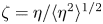 $\zeta = \eta / \langle \eta ^{2} \rangle ^{1/2}$ is normally distributed with zero mean and unit variance (see § 4.2), such that the variables
 $\zeta ^{3}$ (corresponding to the skewness) and
 $\zeta ^{4}$ (corresponding to the kurtosis) have variances
 $15$ and
 $96$, respectively. It then follows that the uncertainty of the kurtosis is expected to be
 $(96/15)^{1/2} \approx 2.5$ times larger than the uncertainty of the skewness when using the same number of measurements, since the confidence interval for any particular quantity scales with its respective standard deviation. We note that an interesting corollary of this short argument is that approximately
 $96/15 = 6.4$ times as many measurements are needed to obtain the kurtosis with the same uncertainty as the skewness, because the width of the confidence interval is inversely proportional to the square root of the number of measurements.
(a) The skewness  $\mathcal {S}$ and (b) the kurtosis
 $\mathcal {K}$ as a function of time. The simulated results are averages of 20 realizations of the initial condition, and the legend applies to both figures.

Now, after the initial ramping period (i.e. approximately the first 10 peak periods) a larger value of  $\varepsilon _0$ is clearly seen to yield a larger skewness, which is in line with the well-known fact that troughs flatten and crests sharpen as the steepness is increased. In all cases, except for
 $\varepsilon _0 = 0.05$ where the statistical noise is too large to make the conclusion, the skewness decreases with time after the initial ramping period. For large values of
 $\varepsilon _0$ the skewness decays more rapidly than for small values of
 $\varepsilon _0$, which is explained by the fact that the steepness decreases most rapidly when
 $\varepsilon _0$ is large cf. figure 1(b).
From figure 2(b) it can be seen that at a fixed point in time, a larger value of  $\varepsilon _0$ leads to a larger kurtosis. Also, when neglecting the oscillations due to statistical noise, it appears that
 $\mathcal {K}$ approaches a steady state level for all values of
 $\varepsilon _0$, although the time at which the level is reached depends on
 $\varepsilon _0$. This hints that the wave fields considered in this work are driven away from their initial Gaussian state by bound wave nonlinearities. For had the nonlinear interactions among the free waves been significant, the kurtosis should first have reached a local maximum before decaying to a quasi-steady state (see e.g. Onorato et al. Reference Onorato, Cavaleri, Fouques, Gramstad, Janssen, Monbaliu, Osborne, Pakozdi, Serio and Stansberg2009; Toffoli et al. Reference Toffoli, Gramstad, Truelsen, Monbaliu, Bitner-Gregersen and Onorato2010; Xiao et al. Reference Xiao, Liu, Wu and Yue2013). We note that the free wave interactions are absent due to the short crestedness (or, equivalently, large directional spread) of the wave fields considered in this work. In fact, Onorato et al. and Toffoli et al. have shown from experiments and numerical simulations, respectively, that the kurtosis of wave fields whose directional spreading is given by the function
 $D(\theta ) = \cos ^{N} (\theta )$ is only affected by free waves when
 $N \ge 90$ up to values of 0.16 for the wave steepness. In that connection it is of course interesting to note that the contribution of the free waves to the kurtosis in our results is very small even for the steepness
 $\varepsilon _0 = 0.30$, since this contribution is of third order, and therefore should become substantial if just the wave steepness is large enough.
4.2. Distribution of the surface elevation
We now consider the PDF of the surface elevation at a fixed point in time, and investigate how this function changes with the initial steepness  $\varepsilon _0$. In addition we compare our results with the theoretical result of Longuet-Higgins (Reference Longuet-Higgins1963), who calculated the PDF of the surface elevation in terms of a Gram–Charlier series based on the cumulants of
 $\eta$. Since the instantaneous value of the steepness has been shown to depend on time, we start, however, by considering how the PDF of the surface elevation changes with time for a fixed
 $\varepsilon _0$ and whether it only depends on the instantaneous value of
 $\varepsilon (t)$.
4.2.1. Dependence on time and the instantaneous steepness
As the PDF of the surface elevation depends on the instantaneous steepness,  $\varepsilon (t)$, it, strictly speaking, does not stay constant during our simulations. To quantify the change over time for different values of
 $\varepsilon _0$, we consider the PDF,
 $p(\zeta )$, of the dimensionless surface elevation
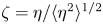 $\zeta = \eta / \langle \eta ^{2} \rangle ^{1/2}$ at times
 $t = 20T_p$,
 $t = 50T_p$ and
 $t = 100 T_p$ for
 $\varepsilon _0 = 0.05$ and
 $\varepsilon _0 = 0.30$, since the former represents the most stationary case and the latter represents the case which changes the most. The PDF of
 $\zeta$ for
 $\varepsilon _0 = 0.05$ at the three times is shown in figure 3(a), and from this it is clear that the PDF changes only very little with time, and we therefore consider it to be constant over time. On the other hand, figure 3(b) shows that the PDF of
 $\zeta$ for
 $\varepsilon _0 = 0.30$ does change over time, most notably for large negative values of
 $\zeta$. We note that for negative values of
 $\zeta$, the change of the PDF becomes visible on the scale of the figure when
 $p(\zeta ) \lesssim 10^{-2}$ while for positive values of
 $\zeta$ the change can be seen in the figure when
 $p(\zeta ) \lesssim 10^{-5}$.
The PDF of  $\zeta$ for (a)
 $\varepsilon _0 = 0.05$ and (b)
 $\varepsilon _0 = 0.30$ at times
 $t = 20T_p$,
 $t = 50T_p$ and
 $t = 100T_p$. The legend applies to both figures, which have been computed using data from 20 realizations of the initial condition. The dashed line depicts the PDF of a normal distribution with zero mean and unit variance for reference.

4.2.2. Representative cases and comparison to theory
We now consider the PDF of the surface elevation at time  $t = 50T_p$, and investigate how this function changes with
 $\varepsilon _0$. From the previous section it is clear that this choice of
 $t$ is somewhat arbitrary since the PDF of
 $\zeta$ varies with time in the steepest cases, and that results which are quantitatively slightly different could have been obtained by choosing a different time. On the other hand, the kurtosis has cf. figure 2(b) reached its quasi steady value at
 $t = 50T_p$ for all values of
 $\varepsilon _0$, and in that sense our investigation of the PDF of the surface elevation is similar to the investigation of Toffoli et al. (Reference Toffoli, Gramstad, Truelsen, Monbaliu, Bitner-Gregersen and Onorato2010), who determined the PDF at the instant where the maximum kurtosis was recorded. For completeness we mention that at
 $t = 50T_p$ the values of the instantaneous steepness for wave fields with
 $\varepsilon _0 = 0.05$, 0.10, 0.15, 0.20, 0.25, 0.30 have decreased to
 $\varepsilon (50T_p) =$ 0.05, 0.10, 0.14, 0.19, 0.22 and 0.25, respectively, in our simulations.
In addition to investigating the role played by  $\varepsilon _0$, we also assess the accuracy of the PDF obtained analytically by Longuet-Higgins (Reference Longuet-Higgins1963). He calculated the PDF of the surface elevation in terms of a Gram–Charlier series, and upon assuming
 $\langle \eta \rangle = 0$, his result for the PDF of the non-dimensionalized surface elevation
 $\zeta$ reads
 \begin{align} p(\zeta) = \frac{1}{(2{\rm \pi})^{1/2}} \exp\left( -\frac{\zeta^{2}}{2} \right) \left( 1 + \frac{1}{6} \varLambda_3 H_3 (\zeta) + \left( \frac{1}{24}\varLambda_4 H_4(\zeta) + \frac{1}{72} \varLambda_3^{2} H_6(\zeta) \right) + \cdots\right), \end{align}
where  $\varLambda _3 = \langle \eta ^{3} \rangle / \langle \eta ^{2} \rangle ^{3/2}$ and
 $\varLambda _4 = \langle \eta ^{4} \rangle / \langle \eta ^{2} \rangle ^{2} - 3$ denote the non-dimensional third- and fourth-order cumulants of the surface elevation, which we estimate from simulation data. Moreover,
 $H_3(\zeta )$,
 $H_4(\zeta )$ and
 $H_6(\zeta )$ are the probabalists’ Hermite polynomials of degree three, four and six defined by
 \begin{gather} H_3 (\zeta) = \zeta^{3} - 3 \zeta, \end{gather}
 \begin{gather}H_4 (\zeta) = \zeta^{4} - 6\zeta^{2} + 3, \end{gather}
 \begin{gather}H_6 (\zeta) = \zeta^{6} - 15\zeta^{4} + 45\zeta^{2} - 15. \end{gather}
In what follows, we will refer to  $p(\zeta )$ as being of
 $n$th order when keeping the first
 $n$ terms (the parenthesis containing
 $H_4$ and
 $H_6$ counts as one term) of the Hermite series. The first-order distribution is thus the well-known Gaussian distribution which is implied by the central limit theorem in the case where the surface consists of a large number of statistically independent components. The second-order distribution is seen to take the effect of skewness into account (clearly
 $\varLambda _3 = \mathcal {S}$), while the third-order distribution also, among other things, allows a non-zero kurtosis.
Our results for  $p(\zeta )$ for different values of
 $\varepsilon _0$ at time
 $t = 50T_p$ are shown in figure 4. For
 $\varepsilon _0 = 0.05$ the PDF is almost symmetrical around
 $\zeta = 0$, and for the inequality
 $p(\zeta ) \ge 10^{-6}$ to be satisfied,
 $\zeta$ must, to a good approximation, lie in the interval
 $[-5, 5]$. For larger values of
 $\varepsilon _0$, the PDF becomes increasingly positively skewed, and as a consequence the inequality
 $p(\zeta ) \ge 10^{-6}$ implies that
 $\zeta$ should be contained in the interval
 $[-3.8, 6.3]$ for
 $\varepsilon _0 = 0.30$. While the mean value of
 $\zeta$ is less than
 $10^{-4}$ in magnitude in all cases, the tail of
 $p(\zeta )$ decays much more rapidly when
 $\varepsilon _0$ is small than when
 $\varepsilon _0$ is large. This fact is reflected by the probabilities listed in tables 1 and 2, which directly show that it is much more likely to find large surface elevations when
 $\varepsilon _0$ is large than when
 $\varepsilon _0$ is small.
The simulated and theoretical PDFs of the non-dimensional surface elevation 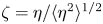 $\zeta = \eta / \langle \eta ^{2} \rangle ^{1/2}$ for (a)
 $\varepsilon _0 = 0.05$, (b)
 $\varepsilon _0 = 0.10$, (c)
 $\varepsilon _0 = 0.15$, (d)
 $\varepsilon _0 = 0.20$, (e)
 $\varepsilon _0 = 0.25$ and (f)
 $\varepsilon _0 = 0.30$ all at time
 $t = 50T_p$. Each histogram is constructed from 20 realizations of the initial condition. The legend applies to all figures.

The probability of  $\zeta$ being larger than 2, 3, 4 and 5, respectively, obtained from simulations and the first-, second- and third-order PDFs from (4.1) for
 $\varepsilon _0 =$ 0.05, 0.10 and 0.15. For the simulated results of the form
 $a \pm b$,
 $b$ denotes the half-width of the 95 % confidence interval. In most cases the statistical uncertainty is smaller than the error introduced when rounding the probabilities to two significant digits, and confidence intervals have therefore been left out. The simulated results are obtained at time
 $t = 50T_p$ from 20 realizations of the initial condition.

Same as table 1 but with  $\varepsilon _0 =$ 0.20, 0.25 and 0.30.

Figure 4 also shows the first-, second- and third-order results of (4.1) for  $p(\zeta )$, and it is clear that for
 $\varepsilon _0 = 0.05$ all three orders provide a highly accurate approximation of the simulated result. For larger values of
 $\varepsilon _0$ the accuracy depends on the order of the approximation, with the third-order result being the most accurate in all cases, although it behaves strangely for large negative values of
 $\zeta$. It is interesting to note that even the third-order PDF underestimates the simulated results, given that the system is driven away from its Gaussian state by bound wave nonlinearities for all values of
 $\varepsilon _0$ as discussed in § 4.1. To quantify the accuracy of the approximate distributions, we have used them to compute the probability that
 $\zeta$ is larger than 2, 3, 4 or 5 for different values of
 $\varepsilon _0$. The results are shown in tables 1 and 2, and from it we conclude as follows: The first-order PDF always underpredicts the probability from the simulations, and it does so by factors which are at least (for
 $\varepsilon _0 = 0.05$) 1.04, 1.4, 1.8 and 2.6 and at most (for
 $\varepsilon _0 = 0.30$) 1.3, 2.7, 9.7 and 75.9 for
 $\zeta \ge 2$,
 $\zeta \ge 3$,
 $\zeta \ge 4$ and
 $\zeta \ge 5$, respectively. The second-order PDF almost predicts the same probability for
 $\zeta \ge 2$ as the simulation, and otherwise it always underestimates the probability obtained from the simulations. For
 $\varepsilon _0 = 0.05$ the probability of the events
 $\zeta \ge 3$,
 $\zeta \ge 4$ and
 $\zeta \ge 5$ are underestimated by factors of 1.4, 1.8 and 2.6, while for
 $\varepsilon _0 = 0.30$ the same events are underestimated by factors of 2.7, 9.7 and 22.0, respectively. Finally, the third-order result agrees very well with the simulations for both
 $\zeta \ge 2$ and
 $\zeta \ge 3$. It predicts the probability of the event
 $\zeta \ge 4$ correctly within 30 % for all values of
 $\varepsilon _0$, while it maximally underestimates the probability of
 $\zeta \ge 5$ by a factor of 3.5, which happens for
 $\varepsilon _0 = 0.30$.
4.3. Distribution of crest height
Next we consider the distribution of the crest height as a function of  $\varepsilon _0$. We compute the PDF of the crest height from time series of the surface elevation at approximately 2300 fixed points in space, arranged such that the minimum distance between two points is at least one peak wavelength, and only data for which
 $20 T_p \le t \le 100T_p$ are used such that the initial ramping period does not influence the result. For each time series the surface elevation is said to have a crest at time
 $t_n = n{\rm \Delta} t$ of height
 $\eta _c = \eta (t_n)$ if
 $\eta (t_n) > \eta (t_{n \pm 1})$, and we note that crest heights may be negative with this definition. As such, it differs from the usual definition used in connection with zero-crossing analyses, where a crest is defined as the highest point of an individual wave. If one insists that a crest height must be positive, we here note that one may simply use the conditional PDF
 \begin{equation} p(\eta_c \,|\, \eta_c \ge 0) = \frac{p(\eta_c)}{\displaystyle\int_{0}^{\infty} p(\eta_c) \,{{\textrm{d}}} \eta_c} \end{equation}
in connection with our definition of a crest. In the following, we will, however, not pursue this possibility, as we restrict our attention to the dependence of  $p(\eta _c)$ on the steepness, and how well the theoretical distributions of Longuet-Higgins (Reference Longuet-Higgins1964) and Tayfun (Reference Tayfun1980) compare to the simulation results.
The result of Longuet-Higgins builds on the work of Cartwright & Longuet-Higgins (Reference Cartwright and Longuet-Higgins1956) and Longuet-Higgins (Reference Longuet-Higgins1963), and gives the PDF of  $\eta _c$ per unit time. Normalizing by the total number of crests per unit time for the case where
 $\varepsilon _0 = 0$, one finds that the distribution of
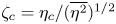 $\zeta _c = \eta _c / (\overline {\eta ^{2}})^{1/2}$ to second order (i.e. including the effects of skewness) is given by
 \begin{align} p_{{LH}}(\zeta_c) &= \left(\frac{1 - \rho^{2}}{2{\rm \pi}} \right)^{1/2} \left( \textrm{e}^{-x^{2}/2} - \rho x F(x; \rho) \vphantom{\frac{1}{6}}\right.\nonumber\\ &\quad + \frac{1}{6} \varLambda_{300} \left( \left( \left(1-\rho^{2}\right)^{3} x^{3} - \left(3 - 9\rho^{2} + 5\rho^{4} \right) x \right) \textrm{e}^{-x^{2}/2} \right.\nonumber\\ &\quad \left.- \left( \rho \left( 1 - \rho^{2} \right)^{3} x^{4} - 6 \rho \left(1-\rho^{2}\right)^{2} x^{2} + 3\rho \left(1-\rho^{2}\right) \right) F(x;\rho) \right) \nonumber\\ &\quad + \frac{1}{2} \varLambda_{201} \left( \rho \left( 2- \rho^{2} \right) x \,\textrm{e}^{-x^{2}/2} + \left( \left(1-\rho^{2}\right)^{2} x^{2} - \left(1-\rho^{2}\right) \right) F(x; \rho) \right) \nonumber\\ &\quad + \frac{1}{2} \varLambda_{102} x \,\textrm{e}^{-x^{2}/2} + \frac{1}{6} \varLambda_{003} \rho x \,\textrm{e}^{-x^{2}/2} \nonumber\\ &\quad \left. -\frac{1}{2} \varLambda_{120} \left( \left(1-\rho^{2}\right) x \,\textrm{e}^{-x^{2}/2} + \left(\rho - \rho x^{2} + \rho^{3} x^{2}\right) F(x; \rho) \right)\right) \end{align}
after correcting a few printing errors as well as an issue with the definition of the skewness coefficients in the paper by Longuet-Higgins (Reference Longuet-Higgins1964). Here the numbers  $x$ and
 $\rho$ and the function
 $F(x;\rho )$ are defined as
 \begin{align} x = \frac{\zeta_c}{\left( 1 - \rho^{2} \right)^{1/2}},\quad \rho = \frac{\overline{\eta \eta_{tt} }}{\left(\overline{\eta^{2}}\, \overline{\eta_{tt}^{2} } \right)^{1/2}},\quad F(x;\rho) = \exp\big({-x^{2} (1- \rho^{2} )/2}\big) \int_{\rho x}^{\infty} \textrm{e}^{-z^{2}/2} \,{{\textrm{d}}}z, \end{align}
while the different skewness coefficients are given by
 \begin{equation} \varLambda_{p_1 p_2 p_3} = \frac{(-1)^{p_3}}{\left(1-\rho^{2}\right)^{(p_1 + p_3)/2}} \frac{\overline{\eta_{\vphantom{t}}^{p_1} \eta_{t}^{p_2} \eta_{tt}^{p_3}}}{\left( \overline{\eta^{2}}\right)^{p_1/2} \left( \overline{\eta_{t}^{2}} \right)^{p_2/2} \left( \overline{\eta_{tt}^{2}} \right)^{p_3/2}}. \end{equation}
To compute these coefficients, we use a centred second-order finite difference scheme to compute the time derivatives of  $\eta$. In what follows we say that
 $p_{{LH}}(\zeta _c)$ is of first order when all skewness terms in (4.4) are neglected, and of second order if the entire expression is used, and we note that the first order result for
 $p_{{LH}}(\zeta _c)$ is the exact result for the PDF of the crest height in the limit
 $\varepsilon _0 \rightarrow 0$.
The result of Tayfun is based on the assumption that the wave field is unidirectional with an underlying narrowbanded frequency spectrum and is accurate to second order in wave steepness. In the present notation the expression for the PDF reads
 \begin{equation} p_{{T}}(\zeta_c) = \frac{2}{\varepsilon} \left( 1 - \frac{1}{\left( \varepsilon \zeta_c + 1\right)^{1/2}} \right) \exp \left( - \frac{2}{\varepsilon^{2}} \left( \left( \varepsilon \zeta_c + 1 \right)^{1/2} - 1 \right)^{2} \right), \end{equation}
and we have evaluated it taking  $\varepsilon = \varepsilon _0$. Using a Taylor series expansion, it is straightforward to show that this expression reduces to the well-known Rayleigh distribution
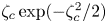 $\zeta _c \exp (- \zeta _c^{2} / 2)$ for narrowbanded waves as
 $\epsilon$ becomes vanishingly small, and we note that this is fundamentally different from the crest height distribution of Longuet-Higgins, which reduces to the exact result in the linear limit. For a discussion and illustration of the difference between the PDFs in the linear limit we refer to the paper by Cartwright & Longuet-Higgins (Reference Cartwright and Longuet-Higgins1956).
Our results for  $p(\zeta _c)$ are shown for different values of
 $\varepsilon _0$ in figure 5, which illustrates the fact that the PDF becomes more skewed towards positive values of
 $\zeta _c$ as
 $\varepsilon _0$ increases. This may be seen quantitatively by noting that for the inequality
 $p(\zeta _c) \ge 10^{-6}$ to be approximately satisfied,
 $\zeta _c$ must lie in the interval
 $[-2, 6]$ when
 $\varepsilon _0 = 0.05$ and in the interval
 $[-2, 7.5]$ when
 $\varepsilon _0 = 0.30$. The mean crest height varies only little with
 $\varepsilon _0$, and achieves its minimum, 1.10, for
 $\varepsilon _0 = 0.05$ and its maximum, 1.17, for
 $\varepsilon _0 = 0.20$. In contrast, the mode (i.e. the most probable value of
 $\zeta _c$) of the crest height distribution monotonically increases in an approximately linear fashion with
 $\varepsilon _0$, and is 0.77 for
 $\varepsilon _0 = 0.05$ and 0.89 for
 $\varepsilon _0 = 0.30$.
The simulated and theoretical PDFs of the non-dimensional crest height 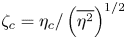 $\zeta _c = \eta _c/ \left(\overline {\eta ^{2}}\right)^{1/2}$ for (a)
 $\varepsilon _0 = 0.05$, (b)
 $\varepsilon _0 = 0.10$, (c)
 $\varepsilon _0 = 0.15$, (d)
 $\varepsilon _0 = 0.20$, (e)
 $\varepsilon _0 = 0.25$ and (f)
 $\varepsilon _0 = 0.30$. Each histogram is constructed from 20 realizations of the initial condition and uses data from the time interval
 $20 \le t \le 100T_p$. The legend applies to all figures.

The theoretical results of Longuet-Higgins and Tayfun are also shown in the figure, and from these we conclude the following: The first-order PDF of Longuet-Higgins is relatively accurate for  $\varepsilon _0 = 0.05$ only, as it overestimates the probability density of large negative crest heights and drastically underestimates the probability density of large positive crest heights larger for values of
 $\varepsilon _0$. The second-order PDF of Longuet-Higgins shares these drawbacks, but is somewhat more accurate than the first-order distribution. In neither case do we consider a more quantitative comparison necessary to conclude that the two PDFs are not useful to predict the probability of large crest heights in steep wave fields. Finally, the second-order PDF of Tayfun is not capable of predicting negative crest heights due to the narrowband assumption, but predicts the probability density of large positive crest heights for large values of
 $\varepsilon _0$ with very high accuracy. This is remarkable when considering that the PDF is derived for unidirectional wave fields with a narrowbanded frequency spectrum while the wave fields in this work are short-crested and the underlying JONSWAP spectrum is not exactly narrowbanded. The good agreement is, however, not completely unexpected, as e.g. Onorato et al. (Reference Onorato, Cavaleri, Fouques, Gramstad, Janssen, Monbaliu, Osborne, Pakozdi, Serio and Stansberg2009) have previously demonstrated that the Tayfun distribution performs well for wave fields whose statistical properties are dominated by bound wave effects.
4.4. Average surface elevation around large crests
We conclude the study of the statistical properties of the surface elevation by considering the average surface elevation around large crests at a fixed point in time. This is an old problem to which, among others, Phillips, Gu & Donelan (Reference Phillips, Gu and Donelan1993) and Boccoti (Reference Boccoti2000) have contributed solutions to lowest order in  $\varepsilon _0$, and Fedele & Tayfun (Reference Fedele and Tayfun2009) have supplied a solution that incorporates weak nonlinearity. Here we define the surface elevation to have a crest at the location
 $(x_c, y_c)$ with height
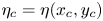 $\eta _c = \eta (x_c, y_c)$ if
 $\eta _c \ge \eta (x,y)$ for all
 $(x,y)$ satisfying the conditions
 $|x - x_c| \le \lambda _p/2$ and
 $|y - y_c| \le \lambda _p/2$, and we compute the average surface elevation around crests with
 $\eta _c \ge H_{m0}$ using data for which
 $t \ge 20T_p$.
The result of the computation for  $\varepsilon _0 = 0.05$ and
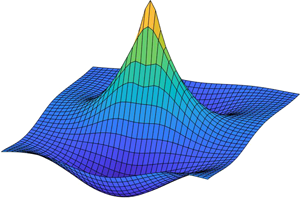
 $\varepsilon _0 = 0.30$ is shown in figure 6, from which it may be seen that large crests, on average, become steeper and more narrow as
 $\varepsilon _0$ increases. Moreover, the trough behind the crest (i.e. for
 $x < x_c$) is seen to flatten and to come closer to the still water level for larger steepness. To make the structure of large crests more clear, their contours are shown in figures 7(a) and 7(b). The figures illustrate the fact that the average surface elevation around large crests does, to a good approximation, possess the symmetry properties
 $\eta (x,y) = \eta (-x,-y)$,
 $\eta (x,y) = \eta (-x,y)$ and
 $\eta (x,y) = \eta (x,-y)$ when
 $\varepsilon _0$ is small, while it only satisfies the condition
 $\eta (x,y) = \eta (x,-y)$ when
 $\varepsilon _0$ is large. We note that the former result can be explained qualitatively by the approximate result of Phillips et al., which states that the surface elevation in the vicinity of a point where
 $\eta$ is known to be large is expected to have the shape of the surface elevation's autocorrelation function,
 \begin{equation} \varPsi(x, y) = \text{E}[\eta(x_0,y_0) \eta(x_0 + x, y_0 + y)], \end{equation}
where  $\text {E}[\cdot ]$ denotes an average over all points
 $(x_0,y_0)$. Since all points of the wave field are statistically identical,
 $\varPsi$ does not depend on
 $x_0$ and
 $y_0$, and one may, for fixed values of
 $x$ and
 $y$, substitute
 $x_0$ with
 $x_0 - x$ and
 $y_0$ with
 $y_0 - y$, which upon insertion in (4.8) shows that
 $\varPsi (x,y) = \varPsi (-x, -y)$. The two other symmetry properties may be shown in an analogous way by utilizing the fact that the directional spreading function (2.3) satisfies the condition
 $D(\theta ) = D(-\theta )$.
The average surface elevation in the domain  $\{ (x,y) \, | \, |x - x_c| \le \lambda _p \ \text {and}\ |y-y_c| \le \lambda _p \}$ around crests higher than
 $H_{m0}$ for (a)
 $\varepsilon = 0.05$ and (b)
 $\varepsilon = 0.30$ seen from behind (i.e. for
 $x < x_c$). The vertical scale on the figures is the same. The figures are computed using data from 20 realizations of the initial condition at times later than
 $20 T_p$.

(a,b) Contour lines of the average surface elevation in the domain  $\{ (x,y) \, | \, |x - x_c| \le \lambda _p \ \text {and}\ |y-y_c| \le \lambda _p \}$ around crests higher than
 $H_{m0}$ for (a)
 $\varepsilon = 0.05$ and (b)
 $\varepsilon = 0.30$. The crest elevation has been normalized to 1. (c,d) Comparison of the average surface elevation around crests higher than
 $H_{m0}$ and the autocorrelation function (4.8) computed at
 $t = 50T_p$ for (c)
 $\varepsilon _0 = 0.05$ and (d)
 $\varepsilon _0 = 0.30$. The legend applies to both (c) and (d). The figures are computed using data from 20 realizations of the initial condition at times later than
 $20 T_p$.

In order to check the actual accuracy of the approximate result of Phillips et al., the average surface elevation around crests higher than  $H_{m0}$ is compared to the autocorrelation function along the line
 $y = y_c$ for
 $\varepsilon _0 =$ 0.05 and 0.30 in figures 7(c) and 7(d). For
 $\varepsilon _0 = 0.05$ the overall agreement is seen to be good, although the autocorrelation function predicts the troughs to be slightly deeper than found from the simulation results. For
 $\varepsilon _0 = 0.30$ the agreement is in contrast very poor. The autocorrelation function severely overpredicts the depth of the troughs and does also not capture the shape of the crest. Moreover, the autocorrelation function predicts the average surface elevation around the crest to be symmetrical, which it clearly is not.
5. Statistical properties of fluid kinematics at the surface
In this section we study the horizontal fluid velocity at the surface,  $v_h^{(s)}$, the horizontal fluid acceleration at the surface,
 $a_h^{(s)}$, and the vertical fluid acceleration at the surface,
 $a_z^{(s)}$, at a fixed point in time as a function of the initial steepness. These quantities are defined as
 \begin{gather} v_h^{(s)} = \left.\left(v_x^{2} + v_y^{2} \right)^{1/2}\right|_{z = \eta}, \end{gather}
 \begin{gather}a_h^{(s)} = \left.\left(a_x^{2} + a_y^{2} \right)^{1/2}\right|_{z = \eta}, \end{gather}
 \begin{gather}a_z^{(s)} = a_z |_{z = \eta}, \end{gather}
and we normalize them by  $v_0 = \varepsilon _0 (g/k_p)^{1/2}$ and
 $a_0 = \varepsilon _0 g$, respectively, where the factor
 $\varepsilon _0$ is included in each case to account for the expected scaling based on linear theory. Although the statistical properties of the wave field change slightly in time, we will again use the results at
 $t = 50T_p$ as a representative of the results for all
 $t$ satisfying
 $20 T_p \le t \le 100T_p$, as we did in § 4.2. Since we have not been able to find a discussion of the PDFs of
 $v_h^{(s)}$ and
 $a_h^{(s)}$ in the literature and
 $a_z^{(s)}$ has also not received much attention, we start by deriving the PDFs of
 $v_h^{(s)}$,
 $a_h^{(s)}$ and
 $a_z^{(s)}$ based on first-order theory using some results obtained by Song & Wu (Reference Song and Wu2000) in order to find out what to expect in the limit of small steepness. Using our simulation results we then go on to discuss how the exact PDFs depend on
 $\varepsilon _0$ and how they differ from the first-order results. Finally, we consider the joint distribution of the fluid kinematics at the surface and the surface elevation, and ask for what surface elevations velocities and accelerations of large magnitude occur. We note that this question is motivated by the work of Sergeeva & Slunyaev (Reference Sergeeva and Slunyaev2013), who investigated whether large fluid velocities at the surface only occur in connection with large surface elevations.
Before proceeding, we want to draw attention to the fact that the distributions of the fluid kinematics presented in this paper are not expected to be exhaustive descriptions of the true distributions that may be measured in field experiments, since the effects of wave breaking are not included in our simulations. In particular caution should be taken for the wave fields with large values of  $\varepsilon _0$ where breaking is expected to occur more often than for wave fields with small values of
 $\varepsilon _0$. The reason for this warning is that breaking waves have been found to exhibit substantially more violent kinematics than non-breaking waves. For a discussion of the fluid kinematics of breaking waves we refer the reader to the papers by Grue & Jensen (Reference Grue and Jensen2006) and Alberello et al. (Reference Alberello, Chabchoub, Monty, Nelli, Elsnab and Toffoli2018) as well as the references therein.
5.1. First-order distributions of the surface kinematics
To derive the PDF of  $v_h^{(s)}$ we start out by noting that when only terms to first order in
 $\varepsilon _0$ are kept, (67) of Song & Wu (Reference Song and Wu2000) immediately implies that the horizontal components of the fluid velocity at the surface,
 $v_x^{(s)}$ and
 $v_y^{(s)}$, are jointly normally distributed. Since the directional spreading function (2.3) of the wave fields studied in this work possesses the symmetry property
 $D(\theta ) = D(-\theta )$, it follows from (34) of Song & Wu that
 $v_x^{(s)}$ and
 $v_y^{(s)}$ are uncorrelated, and their joint PDF can hence be expressed generically as
 \begin{equation} p \left( v_x^{(s)}, v_y^{(s)} \right) = \frac{1}{2 {\rm \pi}\sigma_{v_x} \sigma_{v_y}} \exp \left( - \frac{1}{2} \left( \left( \frac{v_x^{(s)}}{\sigma_{v_x}} \right)^{2} + \left( \frac{v_y^{(s)}}{\sigma_{v_y}} \right)^{2} \right) \right), \end{equation}
where  $\sigma _{v_x}$ and
 $\sigma _{v_y}$ denote the standard deviations of
 $v_x^{(s)}$ and
 $v_y^{(s)}$, respectively. By definition, the cumulative distribution function of
 $v_h^{(s)}$ is given by
 \begin{equation} P \left( v_h^{(s)} \le v \right) = \int_{v_x^{(s)^{2}} + v_y^{(s)^{2}} \le v^{2}} p \left( v_x^{(s)}, v_y^{(s)} \right) {{\textrm{d}}}v_x^{(s)} \,{{\textrm{d}}}v_y^{(s)}, \end{equation}
and upon insertion of (5.2), differentiation with respect to  $v$ and some tedious, but otherwise straightforward, algebraic manipulations, it can be shown that the PDF of
 $v_h^{(s)}/v_0$ to first order in
 $\varepsilon _0$ reads
 \begin{align} p \left( v_h^{(s)} / v_0 \right) = \frac{2}{\rm \pi} \frac{v_h^{(s)} v_0}{\sigma_{v_x} \sigma_{v_y}} \int_{0}^{{\rm \pi}/2}\exp \left( - \frac{1}{2} \left( \frac{v_h^{(s)}}{\sigma_{v_x}} \right)^{2} \left( \cos(x)^{2} + \left(\frac{\sigma_{v_x}}{\sigma_{v_y}} \right)^{2} \sin(x)^{2} \right) \right){{\textrm{d}}}x. \end{align}
We note that in the case where  $\sigma _{v_x} = \sigma _{v_y}$ the integral becomes trivial and
 $p( v_h^{(s)} /v_0 )$ is seen to be the PDF of a Rayleigh distribution. In the more general case where
 $\sigma _{v_x} \neq \sigma _{v_y}$ and both standard deviations are non-zero, the integral can not be computed in terms of elementary functions, but the notation may be simplified by using the modified Bessel function of order zero,
 $I_0$. After a few calculations one finds that (5.4) can be rewritten as
 \begin{equation} p \left( v_h^{(s)} / v_0 \right) = \frac{v_h^{(s)} v_0}{\sigma_{v_x} \sigma_{v_y}} \exp \left( - \frac{1}{4} v_h^{(s)^{2}} \left( \frac{1}{\sigma_{v_x}^{2}} + \frac{1}{\sigma_{v_y}^{2}} \right) \right)I_0 \left( \frac{1}{4} v_h^{(s)^{2}} \left( \frac{1}{\sigma_{v_x}^{2}} - \frac{1}{\sigma_{v_y}^{2}} \right) \right), \end{equation}
which is on a form that may be evaluated directly by a large number of software packages. In order to find the standard deviations we have executed simulations with 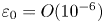 $\varepsilon _0 = O(10^{-6})$, and found that
 $\sigma _{v_x} \approx 0.556 v_0$ and
 $\sigma _{v_y} \approx 0.321 v_0$, such that
 $\sigma _{v_x} / \sigma _{v_y} \approx 1.732$ is very close to the exact ratio
 $\sqrt {3} \approx 1.732$, which may be derived using (33) and (35) of Song & Wu.
To derive the PDF of  $a_h^{(s)}$ we start by noting that the contribution from the nonlinear convective terms to the horizontal components of the fluid acceleration at the surface,
 $a_x^{(s)}$ and
 $a_y^{(s)}$, vanish to first order in
 $\varepsilon _0$. As a consequence,
 $a_x^{(s)}$ and
 $a_y^{(s)}$ are jointly normally distributed to this order, and using the same argument about the symmetry of the directional spreading function as above, their correlation can be shown to be zero. This then implies that the derivation of the PDF of
 $a_h^{(s)}/a_0$ becomes exactly the same as that of
 $p ( v_h^{(s)}/v_0 )$, and we are therefore content with stating the result, which is
 \begin{equation} p \left( a_h^{(s)} / a_0 \right) = \frac{a_h^{(s)} a_0}{\sigma_{a_x} \sigma_{a_y}} \exp \left( - \frac{1}{4} a_h^{(s)^{2}} \left( \frac{1}{\sigma_{a_x}^{2}} + \frac{1}{\sigma_{a_y}^{2}} \right) \right)I_0 \left( \frac{1}{4} a_h^{(s)^{2}} \left( \frac{1}{\sigma_{a_x}^{2}}-\frac{1}{\sigma_{a_y}^{2}} \right) \right). \end{equation}
Here,  $\sigma _{a_x} \approx 0.831 a_0$ and
 $\sigma _{a_x} \approx 0.489 a_0$ are the standard deviations of
 $a_x^{(s)}$ and
 $a_y^{(s)}$, respectively, and the actual values have again been found by simulating wave fields with
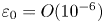 $\varepsilon _0 = O(10^{-6})$. We note that
 $\sigma _{a_x} / \sigma _{a_x} \approx 1.699$ which is close to the expected ratio of
 $\sqrt {3}$ for the directional spreading function (2.3).
Finally, it may readily be seen that  $a_z^{(s)}$ follows a normal distribution to first order in
 $\varepsilon _0$. Hence, the PDF of
 $a_z^{(s)}/a_0$ to this order simply reads
 \begin{equation} p \left( a_z^{(s)} / a_0 \right) = \frac{a_0}{(2{\rm \pi})^{1/2} \sigma_{a_z}} \exp \left( - \frac{1}{2} \left( \frac{a_z^{(s)}}{\sigma_{a_z}} \right)^{2} \right), \end{equation}
where a good approximation for the standard deviation of  $a_z^{(s)}$ has been found to be
 $\sigma _{a_z} \approx 0.950 a_0$ by simulating wave fields with
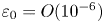 $\varepsilon _0 = O(10^{-6})$. This concludes our derivation of the PDFs of the quantities
 $v_h^{(s)}$,
 $a_h^{(s)}$ and
 $a_z^{(s)}$ to first order.
5.2. Nonlinear distributions of the surface kinematics
We now investigate the PDFs of  $v_h^{(s)}/v_0$,
 $a_h^{(s)}/a_0$ and
 $a_z^{(s)}/a_0$ obtained from our simulations at time
 $t = 50T_p$ for different values of
 $\varepsilon _0$. The PDFs are shown in figure 8, from which it may be seen that the PDFs of
 $v_h^{(s)}/v_0$ and
 $a_h^{(s)}/a_0$ acquire a less rapidly decaying tail as
 $\varepsilon _0$ increases from 0.05 to approximately 0.20, and that the PDFs are almost independent of
 $\varepsilon _0$ when the initial steepness is 0.20 or larger. In contrast, both the left and right tails of the PDF of
 $a_z^{(s)}/a_0$ become more rapidly decaying as
 $\varepsilon _0$ increases. The trend is, however, most pronounced for small values of
 $\varepsilon _0$. The PDFs of all three variables are quantitatively described in table 3 through their modes, mean values and standard deviations. The table shows that the modes and mean values of
 $v_h^{(s)}/v_0$ and
 $a_h^{(s)}/a_0$ decrease with
 $\varepsilon _0$, while the opposite happens to be the case for
 $a_z^{(s)}/a_0$. The table also shows, surprisingly enough, that the standard deviations of all three variables decrease with the initial steepness, and we can therefore in some sense conclude that the fluid kinematics at the surface become more predictable as the initial steepness is increased. This statement should, however, be taken cautiously, as the above description of the PDFs implicitly implies that the probability of finding very large horizontal fluid velocities and accelerations at the surface increases with the steepness.
The PDFs of (a,b)  $v_h^{(s)}/v_0$, (c,d)
 $a_h^{(s)}/a_0$ and (e,f)
 $a_z^{(s)}/a_0$ at time
 $t = 50T_p$ for different values of
 $\varepsilon _0$. The PDFs are computed from 20 realizations of the initial condition. The legends of the first row apply to all rows. The dashed lines depict the first-order results given by (5.5), (5.6) and (5.7), respectively.

The modes, means and standard deviations of  $v_h^{(s)}/v_0$,
 $a_h^{(s)}/a_0$ and
 $a_z^{(s)}/a_0$ at time
 $t = 50T_p$ as a function of
 $\varepsilon _0$. The values are computed from 20 realizations of the initial condition.

In order to assess the accuracy of the first-order results (5.5), (5.6) and (5.7), we show them as dashed lines in figure 8 together with the nonlinear results. From the figure we note that the first-order result for the PDF of  $v_h^{(s)}$ matches the nonlinear results with
 $\varepsilon _0 \le 0.15$ rather well, but also that the first-order results in all other cases deviate substantially from the nonlinear results. In particular we note that for steep wave fields the first-order result tends to underestimate the probability of large values of
 $v_h^{(s)}$ and
 $a_h^{(s)}$ and overestimate the probability of large values of
 $a_z^{(s)}$.
5.3. Joint distribution of surface kinematics and surface elevation
The interest in very large surface and crest elevations is partly motivated by the fact that they are typically accompanied by large fluid velocities and accelerations. There is, however, no guarantee that a violent fluid flow is found only in the vicinity of large surface elevations, since it e.g. has been shown by Sergeeva & Slunyaev (Reference Sergeeva and Slunyaev2013) that not all large fluid velocities at the surface of unidirectional waves are found where the surface elevation is large. In an attempt to find out for what surface elevations large fluid velocities and accelerations at the surface occur, we have computed the joint PDF of  $\eta / H_{m0}$ with each of
 $v_h^{(s)}/v_0$,
 $a_h^{(s)}/a_0$ and
 $| a_z^{(s)} | /a_0$ at time
 $t = 50T_p$ for different values of
 $\varepsilon _0$. The results for
 $\varepsilon _0 = 0.05$ and 0.30 are shown in figure 9, and from it we reach different conclusions about the fluid kinematics at the surface when the initial steepness is small and when it is large. When the initial steepness is small, we conclude that large values of
 $v_h^{(s)}/v_0$ and
 $| a_z^{(s)} | /a_0$ are most likely found when the surface elevation is large in magnitude, while large values of
 $a_h^{(s)}/a_0$ are most likely found when the surface elevation is small in magnitude, i.e. close to the still water level. When the initial steepness is large, we can make the same conclusion about
 $a_h^{(s)}/a_0$, but large values of
 $v_h^{(s)}/v_0$ are now found primarily when the surface elevation is large and positive, whereas large values of
 $| a_z^{(s)} | /a_0$ are mainly found when the surface elevation is large and negative. Even though the fluid velocities and accelerations at the surface are important quantities, we stress at this point that they cannot be expected to give the full picture of how violent the flow field actually is. For example we know from the work of Longuet-Higgins (Reference Longuet-Higgins1986) that when the steepness becomes large enough, the downwards fluid acceleration at the crest of a steady nonlinear wave may in fact be exceeded by up to approximately 20 % by the maximum downwards fluid acceleration found vertically below the crest.
The joint PDFs of  $\eta /H_{m0}$ and (a,d)
 $v_h^{(s)}/v_0$, (b,e)
 $a_h^{(s)}/a_0$ and (c,f)
 $| a_z^{(s)} |/a_0$ at time
 $t = 50T_p$ for
 $\varepsilon _0 = 0.05$ (a–c) and
 $\varepsilon _0 = 0.30$ (d–f). All figures are produced using 20 realizations of the initial condition.

6. Statistical properties of fluid kinematics associated with large crests
In this section we present a detailed analysis of the largest fluid velocities and accelerations appearing in connection with large crests. To do so, we consider the wave field at fixed points in time with  $t \ge 20T_p$, and define the surface elevation to have a crest at the location
 $(x_c, y_c)$ with height
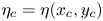 $\eta _c = \eta (x_c, y_c)$ in the same way as in § 4.4, i.e. if
 $\eta _c \ge \eta (x,y)$ for all
 $(x,y)$ satisfying the conditions
 $|x - x_c| \le \lambda _p/2$ and
 $|y - y_c| \le \lambda _p/2$. We consider the extremum velocities and accelerations
 \begin{gather} v_h^{(m)} = {\max} \left\{ \left( v_x^{2} + v_y^{2} \right)^{1/2} \right\}, \end{gather}
 \begin{gather}a_h^{(m)} = {\max} \left\{ \left( a_x^{2} + a_y^{2} \right)^{1/2} \right\}, \end{gather}
 \begin{gather}a_z^{(m)} = {\min} \left\{ a_z \right\}, \end{gather}
where the maxima and minimum are computed over the region of space
 \begin{equation} \left\{ (x,y,z) \,\left|\, |x -x_c| \le \frac{\lambda_p}{2}\right.,\ |y -y_c| \le \frac{\lambda_p}{2} \ \text{and}\ -1.5 H_{m0} \le z \le \eta(x,y) \right\}, \end{equation}
and note that the minimum value of  $a_z$ corresponds to the value having the largest magnitude, since vertical accelerations are negative close to crests. We begin the analysis by studying the influence of
 $\varepsilon _0$ on the conditional distribution of these quantities given that
 $\eta _c \ge H_{m0}$. Next, we consider the distribution of the locations relative to the crest at which
 $v_h^{(m)}$,
 $a_h^{(m)}$ and
 $a_z^{(m)}$ occur for crests higher than
 $H_{m0}$, and show that only the horizontal acceleration attains its maximum away from the crest. For crests higher than
 $H_{m0}$ we therefore subsequently investigate the distribution of the horizontal acceleration at the crest,
 \begin{equation} a_h^{(c)} = \left.\left( a_x^{2} + a_y^{2} \right)^{1/2}\right|_{(x,y,z) = (x_c, y_c, \eta_c)}, \end{equation}
relative to the maximum horizontal acceleration found in connection with the crest.
6.1. Conditional distributions of the extremum velocities and accelerations
Our results for the conditional PDFs of  $v_h^{(m)}/v_0$,
 $a_h^{(m)}/a_0$ and
 $a_z^{(m)}/a_0$ given that
 $\eta _c \ge H_{m0}$ are shown in figure 10 for different values of
 $\varepsilon _0$. For all variables it holds that a larger value of
 $\varepsilon _0$ leads to a less rapidly decaying tail, in such a way that all PDFs are easily told apart on the scale of the figure already around probability densities of magnitude
 $10^{-2}$. For
 $v_h^{(m)}/v_0$ the tail changes most rapidly for
 $\varepsilon _0 \le 0.15$ while for the accelerations the tail also changes appreciably for larger values of
 $\varepsilon _0$. From the figure it is also clear that the most likely values of
 $v_h^{(m)}/v_0$ and
 $a_h^{(m)}/a_0$ are only weakly dependent on the initial steepness while the most likely value of
 $a_z^{(m)}/a_0$ quickly moves towards less negative values as
 $\varepsilon _0$ is increased from 0.05. The PDFs are quantitatively described in table 4, which lists the modes, mean values and standard deviations of the three quantities as a function of
 $\varepsilon _0$. From the table it is interesting to note that the standard deviations of the three quantities increase with the initial steepness, which is the exact opposite trend than exhibited by the fluid velocities and accelerations at the surface as discussed in § 5.2. In this connection it should in particular be noted that while the standard deviations of
 $v_h^{(m)}/a_0$ and
 $a_z^{(m)}/a_0$ merely increase by factors of about 1.2 and 1.6, respectively, when
 $\varepsilon _0$ is increased from 0.05 to 0.30, the standard deviation of
 $a_h^{(m)}/a_0$ increases by a factor of approximately 2.8. Finally, we want to draw attention to the fact that the mean of
 $a_h^{(m)}/a_0$ is smaller in magnitude than the mean of
 $a_z^{(m)}/a_0$ for small values of
 $\varepsilon _0$, while it is the other way around with
 $a_h^{(m)}/a_0$ exceeding
 $a_z^{(m)}/a_0$ by approximately a factor 1.5 in magnitude for
 $\varepsilon _0 = 0.30$.
The conditional PDFs of (a,b)  $v_h^{(m)}/v_0$, (c,d)
 $a_h^{(m)}/a_0$ and (e,f)
 $a_z^{(m)}/a_0$ given that
 $\eta _c \ge H_{m0}$ for different values of
 $\varepsilon$. The PDFs are computed from 20 realizations of the initial condition at times later than
 $20 T_p$. The legends of the first row apply to all rows.

The conditional modes, means and standard deviations of  $v_h^{(m)}/v_0$,
 $a_h^{(m)}/a_0$ and
 $a_z^{(m)}/a_0$ given that
 $\eta _c \ge H_{m0}$ as a function of
 $\varepsilon _0$.

The conditional distributions do, of course, not tell the whole story, as they do not distinguish between crests of different heights as long as they are larger than  $H_{m0}$. It turns out, as one would expect, that if the initial steepness is kept constant, the average values of
 $v_h^{(m)}/v_0$,
 $a_h^{(m)}/a_0$ and
 $a_z^{(m)}/a_0$ tend to grow in magnitude with the crest height, and this fact is illustrated in figure 11. The figure shows the averaged extremum velocity and accelerations
 \begin{gather} V_h(\eta_c; \delta) = \frac{1}{N(\eta_c; \delta)} \sum_{n = 1}^{N(\eta_c; \delta)} v_h^{(m)}(n), \end{gather}
 \begin{gather}A_h(\eta_c; \delta) = \frac{1}{N(\eta_c; \delta)} \sum_{n = 1}^{N(\eta_c; \delta)} a_h^{(m)}(n), \end{gather}
 \begin{gather}A_z(\eta_c; \delta) = \frac{1}{N(\eta_c; \delta)} \sum_{n = 1}^{N(\eta_c; \delta)} a_z^{(m)}(n), \end{gather}
where  $N(\eta _c; \delta )$ is the number of crests with elevation in the interval
 $[\eta _c - \delta , \eta _c + \delta )$,
 $v_h^{(m)}(n)$ is the value of
 $v_h^{(m)}$ at the
 $n$th crest of appropriate elevation and
 $a_h^{(m)}(n)$ and
 $a_z^{(m)}(n)$ are defined similarly. In this connection we note that
 $V_h/v_0$ grows with
 $\eta _c$ at a rate which is nearly independent of
 $\varepsilon _0$ and that
 $A_h/a_0$ grows with
 $\eta _c$ at rate which is highly dependent on
 $\varepsilon _0$. It can also be seen from the figure that the rate at which
 $A_z/a_0$ increases in magnitude with
 $\eta _c$ is almost independent of
 $\varepsilon _0$ for small values of the initial steepness but does depend on
 $\varepsilon _0$ for large values of the initial steepness.
The non-dimensional average extremum velocity and accelerations  $V_h/v_0$,
 $A_h/a_0$ and
 $A_z/a_0$ (full lines) with 95 % confidence intervals (dashed-dotted lines) as a function of the crest height. The averages have been computed in steps of
 $0.02H_{m0}$ with
 $\delta = 0.01H_{m0}$, and the legend applies to all figures.

6.2. Locations of the extremum fluid velocities and accelerations
Next, we consider the location at which  $v_h^{(m)}$,
 $a_h^{(m)}$ and
 $a_z^{(m)}$ occur for crests of height larger than
 $H_{m0}$. We denote these locations by
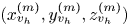 $( x_{v_h}^{(m)}, y_{v_h}^{(m)}, z_{v_h}^{(m)} )$,
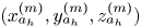 $( x_{a_h}^{(m)}, y_{a_h}^{(m)}, z_{a_h}^{(m)} )$ and
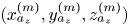 $( x_{a_z}^{(m)}, y_{a_z}^{(m)}, z_{a_z}^{(m)} )$, respectively, and start by examining the location of the horizontal acceleration.
The joint conditional PDF of  $( x_{a_h}^{(m)}, y_{a_h}^{(m)} )$ given that
 $\eta _c \ge H_{m0}$ is shown in figure 12 for different values of
 $\varepsilon _0$, and illustrates the fact that
 $a_h^{(m)}$ is most likely to be found approximately
 $0.1 \lambda _p$ away from the crest in the horizontal plane for all values of
 $\varepsilon _0$. For a small initial steepness,
 $a_h^{(m)}$ is found almost as often behind the crest (i.e. for
 $x_{a_h}^{(m)} < x_c$) as in front of the crest (i.e. for
 $x_{a_h}^{(m)} > x_c$), while for large initial steepness
 $a_h^{(m)}$ is most likely found in front of the crest. Moreover, we note that the conditional PDF becomes more localized with as
 $\varepsilon _0$ increases. Although not to the same degree, the conditional distribution of the vertical location,
 $z_{a_h}^{(m)}$, given that
 $\eta _c \ge H_{m0}$ also becomes more localized as
 $\varepsilon _0$ increases. This may be seen in figure 13, which also shows that the most likely position for
 $a_h^{(m)}$ to occur becomes increasingly negative as
 $\varepsilon _0$ becomes large. As a result the maximum horizontal acceleration is most likely found approximately
 $0.6 H_{m0}$ below the crest when
 $\varepsilon _0 = 0.05$, while for
 $\varepsilon _0 = 0.30$
 $a_h^{(m)}$ occurs most often about
 $0.7H_{m0}$ below the crest. Interestingly enough, the average value of
 $z_{a_h}^{(m)}$ does seemingly not depend on
 $\varepsilon _0$ and is about
 $-0.8H_{m0}$ in all cases.
The joint conditional PDF of  $(x_{a_h}^{(m)}, y_{a_h}^{(m)})$ given that
 $\eta _c \ge H_{m0}$ for (a)
 $\varepsilon _0 = 0.05$, (b)
 $\varepsilon _0 = 0.10$, (c)
 $\varepsilon _0 = 0.15$, (d)
 $\varepsilon _0 = 0.20$, (e)
 $\varepsilon _0 = 0.25$ and (f)
 $\varepsilon _0 = 0.30$.

The conditional PDF of  $z_{a_h}^{(m)}$ given that
 $\eta _c \ge H_{m0}$ for different values of
 $\varepsilon _0$.

In contrast to  $a_h^{(m)}$,
 $v_h^{(m)}$ and
 $a_z^{(m)}$ are typically found right at the crest with a very high probability for all values of the steepness. This fact is illustrated for
 $\varepsilon _0 = 0.15$ in figure 14 which shows the joint conditional PDFs of
 $( x_{v_h}^{(m)}, y_{v_h}^{(m)})$ and
 $(x_{a_z}^{(m)}, y_{a_z}^{(m)})$ given that
 $\eta _c \ge H_{m0}$, and in figure 15 which shows the conditional PDFs of
 $z_{v_h}^{(m)}$ and
 $z_{a_z}^{(m)}$ given that
 $\eta _c \ge H_{m0}$. In this connection it is interesting to note that the maximum horizontal velocity sometimes, although rarely, occurs somewhat below the crest which is never the case for regular waves.
The joint conditional PDFs of (a)  $( x_{v_h}^{(m)}, y_{v_h}^{(m)})$ and (b)
 $( x_{a_z}^{(m)}, y_{a_z}^{(m)})$ given that
 $\eta _c \ge H_{m0}$ for
 $\varepsilon _0 = 0.15$.

The conditional PDFs of (a)  $z_{v_h}^{(m)}$ and (b)
 $z_{a_z}^{(m)}$ given that
 $\eta _c \ge H_{m0}$ for
 $\varepsilon _0 = 0.15$.

6.3. Velocities and accelerations at the crest compared to maximum values
From the preceding section it is clear that the horizontal velocity and vertical acceleration at the crest must typically be very similar to the corresponding maximum quantities associated with the crest. On the other hand, the horizontal acceleration at the crest may deviate substantially from the maximum horizontal acceleration, since the latter is typically found a non-negligible distance away from the crest, and we here quantify the deviation using the conditional PDF of  $a_h^{(c)}/a_h^{(m)}$ given that
 $\eta _c \ge H_{m0}$. Figure 16 illustrates the fact that the PDF acquires a less rapidly decaying tail with the steepness and that it peaks around
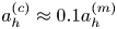 $a_h^{(c)} \approx 0.1 a_h^{(m)}$ for all values of
 $\varepsilon _0$. From integration of the PDF we moreover conclude that the probability of
 $a_h^{(c)}$ exceeding
 $a_h^{(m)}/2$ is less than approximately 1.2 % for
 $\varepsilon _0 = 0.30$ and significantly less for smaller values of the initial steepness.
The conditional PDF of  $a_h^{(c)}/a_h^{(m)}$ given that
 $\eta _c \ge H_{m0}$ for different values of
 $\varepsilon _0$.

7. Conclusions
We have presented a numerical study of the statistical properties of the surface elevation and the fluid kinematics of irregular wave fields with emphasis on the role of the initial wave steepness  $\varepsilon _0$. The study was performed using the fully nonlinear numerical model of Klahn et al. (Reference Klahn, Madsen and Fuhrman2020), which is a pseudospectral volumetric method for solving the irrotational Euler equations without any simplifying assumptions. In that regard this investigation stands out, since most other numerical studies of irregular wave fields have been carried out using either the nonlinear Schrödinger equation (Dysthe et al. Reference Dysthe, Trulsen, Krogstad and Socquet-Juglard2003; Socquet-Juglard et al. Reference Socquet-Juglard, Dysthe, Truelsen, Krogstad and Liu2005), the Zakharov equation (Annenkov & Shrira Reference Annenkov and Shrira2009, Reference Annenkov and Shrira2013, Reference Annenkov and Shrira2018) or a low-order truncation of the HOS method (Toffoli et al. Reference Toffoli, Gramstad, Truelsen, Monbaliu, Bitner-Gregersen and Onorato2010; Xiao et al. Reference Xiao, Liu, Wu and Yue2013; Fedele et al. Reference Fedele, Brennan, Ponce de León, Dudley and Dias2016). The wave fields under consideration were of size
 $50 \lambda _p \times 50 \lambda _p$, discretized with approximately 20 points per peak wavelength and initialized from a directional JONSWAP spectrum using a method due to Tanaka (Reference Tanaka2001).
We first considered the statistical properties of the surface elevation. Its skewness and kurtosis were computed as a function of time, and it was shown that at a fixed point in time a larger value of  $\varepsilon _0$ leads to larger values of the skewness and the kurtosis. Moreover, it was found that while the skewness decreases with time when the steepness is large, the kurtosis seemed to approach a steady state level for all values of
 $\varepsilon _0$. Next, we showed that the PDF of the surface elevation changes slightly over time in our simulations, with the change mainly affecting the left tail of the PDF. With this result in mind, we considered the PDF of the surface elevation at time
 $t = 50T_p$. This PDF was computed for different values of
 $\varepsilon _0$, and it was concluded that it acquires a less rapidly decaying tail for large positive surface elevations as
 $\varepsilon _0$ increases. The simulated results were compared to the first-, second- and third-order approximations of the Gram–Charlier series derived by Longuet-Higgins (Reference Longuet-Higgins1963), and a good agreement was found for all orders for small values of
 $\varepsilon _0$. For large values of
 $\varepsilon _0$ the theoretical results were, however, found to underestimate the probability of large positive surface elevations. Hereafter, we studied the PDF of the crest elevation, whose dependence on the initial steepness was found to be qualitatively similar to that of the PDF of the surface elevation. The theoretical results of Longuet-Higgins (Reference Longuet-Higgins1964) and Tayfun (Reference Tayfun1980) were compared to the simulated results, and while the expressions of Longuet-Higgins did not provide accurate results unless
 $\varepsilon _0 = 0.05$, the expression of Tayfun matched the results of the simulations remarkably well. In that connection it was mentioned that the PDF of Tayfun is based on assumptions which are not satisfied by the wave fields in this work, and it was therefore noted that its good agreement with the simulated results should be regarded as a coincidence. We concluded the investigation of the statistical properties of the surface elevation by considering the expected surface elevation in the vicinity of crests higher than the significant wave height,
 $H_{m0}$. The symmetry properties of the surface elevation were discussed, and it was shown that two out of the three mentioned symmetries are broken as the initial steepness becomes large.
Secondly, we considered various statistical aspects of the fluid kinematics encountered in connection with irregular wave fields. The fluid kinematics of irregular waves have so far only received very little attention in the literature, and none of the PDFs presented in §§ 5 and 6 have to our knowledge been published elsewhere.
In § 5, we first considered the statistical properties of the horizontal fluid velocity and horizontal and vertical fluid acceleration at the surface. Drawing on some results due to Song & Wu (Reference Song and Wu2000) we derived expressions for the PDFs of these quantities to first order, and showed that already for  $\varepsilon _0$ these approximations are fairly inaccurate. When increasing the initial steepness, the tails of the PDFs were found to become less rapidly decaying in the case of the horizontal velocity and acceleration for larger values, and more rapidly decaying in the case of the vertical acceleration. Moreover, the standard deviations of all three quantities were found to become smaller when increasing the value of
 $\varepsilon _0$. Next, we investigated for what surface elevations large fluid kinematics at the surface occur by considering the joint PDF of the surface elevation and the fluid velocities and accelerations. For small values of
 $\varepsilon _0$ we concluded that large horizontal velocities and vertical accelerations at the surface are typically found when the surface elevation is of large magnitude, while large horizontal accelerations at the surface are most often found close to the still water level. For large values of
 $\varepsilon _0$ the latter conclusion still holds, but large horizontal velocities at the surface are in this case most often found when the surface elevation is large and positive, while large vertical accelerations at the surface are most likely found when the surface elevation is large and negative.
In § 6 we characterized the largest values of the horizontal velocity as well as horizontal and vertical accelerations that accompany large crests. We computed the conditional PDFs of these quantities given that the crest height is larger than  $H_{m0}$, and showed that all PDFs acquire less rapidly decaying tails as the initial steepness becomes large. Moreover, we found that the standard deviations of all quantities become larger with
 $\varepsilon _0$ which is in clear contrast to the standard deviations of the fluid velocities and accelerations at the surface. Following this, we studied the statistical distribution of the location where the extremum velocities and accelerations occur. We concluded that for small values of
 $\varepsilon _0$ the largest horizontal acceleration is most likely found the distance
 $0.1 \lambda _p$ either behind or in front of the crest, while for large values of
 $\varepsilon _0$ it is most likely found the same distance in front of the crest. The largest horizontal velocity and vertical acceleration were in all cases most likely to be found right at the crest. Finally, we considered the horizontal acceleration at the crest relative to the maximum horizontal acceleration for crests higher than
 $H_{m0}$. For all values of
 $\varepsilon _0$ we found that the former is most often an order of magnitude smaller than the latter, and that the probability of finding a horizontal acceleration at the crest which is more than half the maximum horizontal acceleration found in connection with the crest is only about 1.2 % in the case
 $\varepsilon _0 = 0.30$ and smaller for smaller values of
 $\varepsilon _0$.
Acknowledgements
The authors gratefully acknowledge the funding received from Centre for Oil and Gas - DTU/Danish Hydrocarbon Research and Technology Centre (DHRTC). Project name: DEWIOS. Project ID: FL_110.
Declaration of interests
The authors report no conflict of interest.



