Introduction
AII amacrine cells are narrow-field amacrine cells with bistratifying processes distributed to the ON and OFF divisions of the inner plexiform layer (IPL) of the retina (Kolb & Famiglietti, Reference Kolb and Famiglietti1974; Strettoi et al., Reference Strettoi, Raviola and Dacheux1992). They receive rod photoreceptor input via the rod bipolar cells that form glutamatergic synapses upon their arboreal dendrites in the inner stratum of the IPL and transmit that signal via gap junctions made by those dendrites upon the terminals of the ON cone bipolar cells, while also releasing glycine from their lobular appendages upon the terminals of the OFF cone bipolar cells (see Demb & Singer, Reference Demb and Singer2012; Marc et al., Reference Marc, Anderson, Jones, Sigulinsky and Lauritzen2014, for review). They can be labeled using antibodies to Parvalbumin, Calretinin, Disabled1, and Prox1, depending upon the species (Pasteels et al., Reference Pasteels, Rogers, Blachier and Pochet1990; Casini et al., Reference Casini, Rickman and Brecha1995; Rice & Curran, Reference Rice and Curran2000; Dyer et al., Reference Dyer, Livesey, Cepko and Oliver2003), with recent attention focusing upon the use of Prox1 to selectively identify them in the amacrine cell division of the inner nuclear layer (INL) (Perez de Sevilla Muller et al., Reference Perez de Sevilla Muller, Azar, de los Santos and Brecha2017). Prox1 is a homeodomain transcription factor shown to play a critical role in retinal proliferation during early development (Dyer et al., Reference Dyer, Livesey, Cepko and Oliver2003), yet it is retained in the somata of horizontal cells, bipolar cells and AII amacrine cells in the mature retina (Perez de Sevilla Muller et al., Reference Perez de Sevilla Muller, Azar, de los Santos and Brecha2017). The Prox1+ AII amacrine cells form a monolayer in the INL adjacent to the IPL, and in wholemount preparations, this permits the imaging of the entire population of AII amacrine cells, from which accurate counts of their total number can be determined (Keeley et al., Reference Keeley, Whitney, Madsen, St John, Borhanian, Leong, Williams and Reese2014), as well as their spatial distribution across the retina (Perez de Sevilla Muller et al., Reference Perez de Sevilla Muller, Azar, de los Santos and Brecha2017).
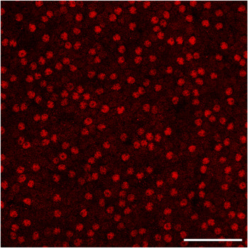
At the global level, AII amacrine cells show relatively little variation as a function of retinal quadrant in the mouse retina, but they exhibit a slight decline in their density in the periphery (Perez de Sevilla Muller et al., Reference Perez de Sevilla Muller, Azar, de los Santos and Brecha2017). At the local level, they have been reported to be distributed as a regular retinal mosaic, evidenced in a single large field of cells (n = 540) assessed using the nearest neighbor (NN) analysis (Perez de Sevilla Muller et al., Reference Perez de Sevilla Muller, Azar, de los Santos and Brecha2017). This sample showed a mean NN distance of 10.1 µm, with a standard deviation of 3.0, from which the regularity index (RI; being the mean NN distance divided by the standard deviation) was calculated to be 3.4. As values such as this are substantially higher than those derived from a theoretical random distribution of points (generating a NNRI of 1.91) (Cook, Reference Cook1996), the mosaic was deemed to be regular, yet this conclusion runs counter to the imaged field in that study, in which there are conspicuous gaps in the field and occasional close pairings of somata (see Fig. 1b of Perez de Sevilla Muller et al., Reference Perez de Sevilla Muller, Azar, de los Santos and Brecha2017). Indeed, our own examination of AII amacrine cells in wholemount preparations reveals comparable results: the mosaic in the mouse retina does not look regular to the eye at all (Fig. 1; see also Keeley et al., Reference Keeley, Whitney, Madsen, St John, Borhanian, Leong, Williams and Reese2014), particularly when compared to the mosaics of cholinergic amacrine cells or horizontal cells (Raven & Reese, Reference Raven and Reese2002; Whitney et al., Reference Whitney, Keeley, Raven and Reese2008). The present investigation examined the organization of the AII amacrine cell population in further detail, using a variety of spatial statistics to understand the somal patterning present in this mosaic.
Materials and methods
The mosaic of AII amacrine cells was analyzed in two different inbred laboratory strains of mice, C57BL/6J (B6/J; n = 7) and A/J (n = 6), obtained from The Jackson Laboratories (Bar Harbor, ME), at ∼6 weeks of age. Mice were given a lethal injection of sodium pentobarbital (120 mg/kg, i.p.), and once deeply anesthetized, they were intracardially perfused with 2–3 ml 0.9% saline followed by ∼50 ml of 4% paraformaldehyde in 0.1 M sodium phosphate buffer (pH 7.2 at 20°C). Eyes were dissected from the orbit and post-fixed for 15 min before being transferred to phosphate buffer. Whole retinas were dissected from the eyes, taking care to ensure that the entirety of the retina was intact, for subsequent immunofluorescence labeling of the AII amacrine cells using an affinity-purified rabbit polyclonal antibody to Prox1 (1:1000; Covance PRB-238C, Princeton, NJ). Primary antibodies were detected using donkey antirabbit secondary IgG conjugated to Cy2 (1:200; Jackson ImmunoResearch Laboratories, West Grove, PA). Whole retinas were mounted under a coverslip and examined on an Olympus microscope equipped with a digital Sony video camera and linked to a computer running Bioquant Nova Prime software (R&M Biometrics, Nashville, TN).
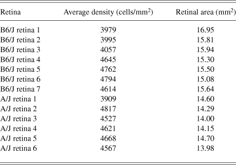
Four fields were sampled per retina, one in each quadrant, centered at a mid-eccentric location, being ∼32,000 µm2 in area. From each of these sampled fields, every Prox1+ AII amacrine cell body was identified using a 20× objective, and from these, the X and Y coordinates for each cell were determined and then exported to a computer running customized software for conducting statistical analyses of 2D spatial point patterns, described elsewhere (Keeley & Reese, Reference Keeley and Reese2014; Keeley et al., Reference Keeley, Kim, Lee, Haverkamp and Reese2017). (A separate study has previously reported the total number of AII amacrine cells derived from these retinas—Keeley et al., Reference Keeley, Whitney, Madsen, St John, Borhanian, Leong, Williams and Reese2014; their average densities, expressed as cells/mm2, along with the total retinal area are indicated here in Table 1, excluding the one retina for which we did not have X, Y coordinates.) From the 2D spatial point pattern for each field, we determined the Voronoi domain (VD) area for every cell, being the territory surrounding each cell that is closer to that cell than to any of its neighbors. We then computed the regularity index derived from these domains, the Voronoi domain regularity index (VDRI), being the mean VD area divided by the standard deviation. We also generated the autocorrelogram (AC) for every field, from which we derived the density recovery profile (DRP) and then computed the effective radius (ER) in order to determine the packing factor (PF), being an index of how closely the mosaic approximates a hexagonal lattice (Rodieck, Reference Rodieck1991), all as described elsewhere (Keeley et al., Reference Keeley, Whitney, Madsen, St John, Borhanian, Leong, Williams and Reese2014, Reference Keeley, Kim, Lee, Haverkamp and Reese2017). The results from the four fields in each retina were then averaged, and animal averages were then used to construct the frequency distributions and histograms shown in the figures.
Density of AII amacrine cells

In addition, for each sampled field we generated a random simulation of cells matched in density, constraining their positioning in the simulation by the size of the AII amacrine cell somata, having previously been determined from a sample of 200 AII amacrine cells to be 7.5 ± 0.5 µm in diameter, using antibodies that reveal the somal membrane (Keeley & Reese, Reference Keeley and Reese2018). The simulations randomly draw soma sizes from a Gaussian distribution with the same mean and standard deviation, where each randomly positioned cell is rejected (with replacement) if it overlaps that of a previously positioned cell, until the number of cells in the simulation matches that for the real field being simulated. We then extracted the X and Y coordinates of these cells for each of those simulated fields, performing the same spatial statistical analyses on those random fields, for direct comparison. One larger field of Prox1+ AII amacrine cells from a B6/J retina was additionally imaged using an Olympus Fluoview1000 laser scanning confocal microscope (Tokyo, Japan), for comparison with Fig. 1b in Perez de Sevilla Muller et al. (Reference Perez de Sevilla Muller, Azar, de los Santos and Brecha2017), illustrated in Fig. 1.
A field of AII amacrine cells in the B6/J retina, revealed by the presence of Prox1 labeling of their nuclei. Scale bar = 50 µm.

Retinal averages were calculated for each spatial statistic and Student’s t-tests were conducted for comparisons between the real data and the density-matched and soma size-constrained random simulations, for both strains. As multiple t-tests were conducted, we have used the Bonferroni correction to ensure a family-wise error rate of P < 0.05.
Results
We have argued elsewhere that understanding the regularity in the spatial patterning of a population of cells must take into consideration both the density as well as the physical size of the cells, for the latter will necessarily constrain the proximity between any two cells, and this constraint upon cellular positioning only increases as a function of cellular density (e.g., Galli-Resta et al., Reference Galli-Resta, Novelli, Kryger, Jacobs and Reese1999; see Reese & Keeley, Reference Reese and Keeley2015, for review). AII amacrine cell bodies, confined to a single stratum at the inner margin of the INL, must necessarily limit their close positioning by a distance comparable to their average soma size, constraining the minimal spacing between cells in the mosaic (Fig. 1). For this reason, we routinely generate random simulations that are matched in density to the real fields but that are constrained by the size of the somata in the real mosaic. It is this difference between the regularity in the real mosaic versus the density-matched and soma-size-constrained random simulation that best captures the degree to which a somal mosaic can be said to be regular (Keeley & Reese, Reference Keeley and Reese2014). Furthermore, we have suggested previously that the NN analysis, by virtue of considering only the distance to the closest neighboring cell, may over-estimate the regularity of a mosaic (e.g., Cook, Reference Cook, Chalupa and Werner2003) when compared to a VD analysis, which takes into consideration the distance of each cell to all of its immediate neighbors (Reese & Keeley, Reference Reese and Keeley2015). We have, consequently, derived our analysis of mosaic regularity from the VD areas for the population of AII amacrine cells.
A direct assessment of the minimal spacing associated with an entire population of neurons is to calculate the ER derived from the DRP (Rodieck, Reference Rodieck1991). The DRP plots the “recovered density” of cells as a function of increasing distance from every cell, where the ER can be considered a size of that minimal spacing present in a mosaic. From the ER derived from every sampled field, we have also computed the PF, another spatial statistic that compares the two-dimensional point pattern to a hexagonal lattice, ranging from 0, a theoretical random distribution of points, to 1.0, a perfect hexagon (Rodieck, Reference Rodieck1991). The present investigation has examined both the VDRI and the PF to describe the spatial features of the AII amacrine cell mosaic, examining fields from all four quadrants of one retina from each mouse, assessed in two different laboratory strains.
In order to compare our data directly to that reported by Perez de Sevilla Muller et al. (Reference Perez de Sevilla Muller, Azar, de los Santos and Brecha2017), we first also measured the NN distances from the population of Prox1+ AII amacrine cells in the 24 and 28 sampled fields from the A/J and B6/J retinas, respectively. From these distances, we calculated the nearest neighbor regularity index (NNRI) for each individual field and found the average across all retinas to be 3.3 for both strains, nearly identical to the value of 3.4 for the single sampled field reported by Perez de Sevilla Muller et al. (Reference Perez de Sevilla Muller, Azar, de los Santos and Brecha2017). Despite the higher average densities in our sampled fields (Table 1), due to the smaller retinal area in these younger (6 week old) mice, the NNRI should be unaffected because it is a scale-independent measure of the patterning in the array of somata. This preliminary comparison would support the contention that we have, in fact, identified the same population analyzed in that study.
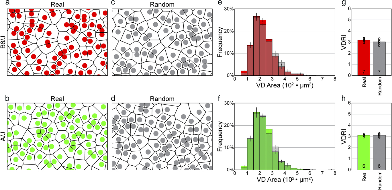
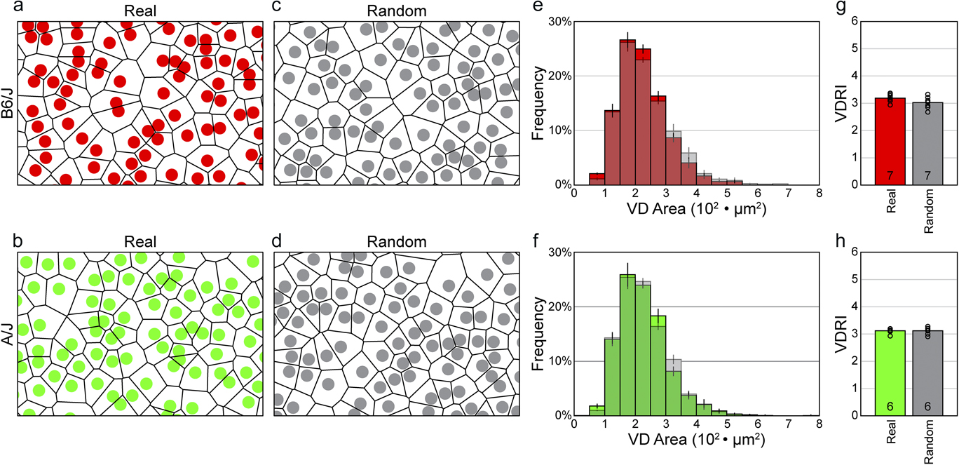
VD analysis, by considering the spatial relationship between each cell and all of its neighbors, provides a more compelling description, both visually as well as statistically, of the patterning present in a two-dimensional point pattern than does the NN analysis (Reese & Keeley, Reference Reese and Keeley2015). The variance in the size of the individual domains in the mosaic (shown in Fig. 2a and 2b) is immediately apparent, and a direct comparison of the average frequency distributions of the Voronoi areas for the real fields versus the random-constrained simulated fields in each strain, (Fig. 2c and 2d), shows that they are nearly identical (compare colored versus shaded distributions in Fig. 2e and 2f). We can also compute the VDRI for the individual sampled fields, and from these we can generate animal averages, for both the real fields and their random simulations. These VDRIs exhibit values that are nearly identical: 3.19 ± 0.06 (mean and SEM) for the real fields and 3.02 ± 0.08 for the random simulations, respectively, for the B6/J strain (the difference was not significant, n.s.), and 3.11 ± 0.04 (real) and 3.11 ± 0.06 (random) for the A/J strain (n.s.) (Fig. 2g and 2h). This VD analysis makes clear that real AII amacrine cell mosaics are no different in their regularity than are simulations matched in density and constrained by soma size, but otherwise random.
(a, b) Spatial point patterns of AII amacrine cells from B6/J (red) and A/J (green) mouse retinas, showing the VD for each individual cell. The fields illustrated were cropped from the larger original sampled fields, showing somata scaled with respect to the field size (and hence Voronoi area). (c, d) Comparable spatial point patterns from random simulations matched in density and soma size to the real distributions. The Voronoi tiling looks comparable to the real mosaics. Cell sizes in a–d are shown as uniformly 7.5 µm in diameter, whereas in reality, as in the density-matched and soma size-constrained random simulations, they vary slightly, having a standard error of 0.5 µm. (e, f) Frequency distributions (mean ± s.e.m.) for the VD areas derived from the sampled retinas and their matched random simulations (shaded), for both strains. (g, h) Histograms showing the mean VDRIs for the real versus random distributions, for both strains. The average VDRI for each retina is indicated with an open circle. Note that the regularity indexes for the real versus random distributions are nearly identical, for both strains.
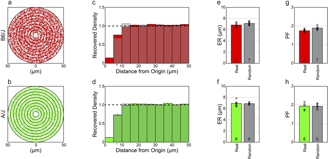
If we compute the spatial AC for these sampled fields of cells, for either strain, we find a vacant region at the origin (Fig. 3a and 3b). The DRP illustrates the variation in average density as a function of distance from the origin of the AC (Fig. 3c and 3d). By computing the DRP for the density-matched and soma size-constrained random simulations and then determining animal averages (for either mouse strain) (shaded histograms in Fig. 3c and 3d), we see that they are nearly identical: the average DRPs for both the real fields and the random simulations each reveal an empty region at the origin that is comparable in size. The size of this “exclusion zone” is indicated by the ER (Rodieck, Reference Rodieck1991), which was determined for every field and then averaged for each retina, being 6.86 ± 0.14 µm (mean and SEM) for the real retinas, versus 7.14 ± 0.11 µm for the random simulations, for the B6/J strain (n.s.), and was 6.92 ± 0.22 µm (real) and 6.91 ± 0.08 µm (random) for the A/J strain (n.s.) (Fig. 2e and 2f). The ER is not, itself, any index of regularity or patterning (Reese & Keeley, Reference Reese and Keeley2015), but in both strains, the size of the ER is no larger than the size of an exclusion zone to be expected by soma size alone, indicating that AII amacrine cells do not space themselves apart farther than a distance required by their physical size. These data in Fig. 2c–2f demonstrate that the frequency of side-by-side pairings of AII amacrine cells is no different than would be expected by chance.
(a, b) Spatial ACs for the two sampled fields from B6/J (red) and A/J (green) mouse retinas shown in Fig. 2a and 2b. Each dot in the AC indicates the positioning of the centroid of the cell with respect to the origin, dot size now being substantially smaller than soma size to permit better resolution between cells. Successive annuli from the origin are at 5 µm intervals. (c, d) DRPs derived from the ACs of the sampled retinas and their density-matched and soma size-constrained random simulations (shaded), for both strains. Each bin indicates the average spatial density at increasing annuli in the ACs, while the horizontal dashed line indicates the expected density of each bin for a theoretical random distribution with no constraints (normalized for each field). Both the real and the soma-size-constrained random distributions show a vacant region at the origin, the “exclusion zone”, appearing comparable in size. Arrowheads indicate the ER in each DRP; these cannot be discriminated between the real and random distributions in the A/J strain. (e, f) Histograms showing the mean ERs for the real versus random distributions, by retina, for both strains. The ER is an index of the size of the exclusion zone revealed in the DRP. (g, h) Histograms showing the mean PF for the real versus random distributions. Note that the PF is nearly identical between the real versus random distributions, for both strains, as should be expected given their comparable ERs. Open circles indicate individual retinal averages for both the ER and PF statistics.

PF analysis was used to assess whether the real mosaic might conceal some level of higher order patterning, for instance, conforming to a lattice that has undergone a degree of jitter, thereby rendering its periodicity in a mosaic undetectable to the eye but revealed in the AC. For instance, simulations of jittered lattices, in certain circumstances, have been shown to possess identical VD statistics to real mosaics containing none of the higher order patterning present in the simulations, though which are hard to distinguish by eye (for example, compare Fig. 2 with 4 of Reese & Keeley, Reference Reese and Keeley2015). But because the PF is derived from the ER, it should be similar, given comparable ERs for the real versus density-matched and soma-size-constrained random conditions, and this was confirmed: the PF was determined to be 0.18 ± 0.003 (mean and SEM; real) versus 0.19 ± 0.003 (random) for the B6/J strain (n.s.) and 0.19 ± 0.007 (real) versus 0.19 ± 0.005 (random) for the A/J strain (n.s.) (Fig. 2g and 2h). These values were far lower than the PFs obtained for either horizontal cells or cholinergic amacrine cells (0.3–0.4), as was also true for the VDRIs indicated above (being 5.0–6.0 for the horizontal and cholinergic amacrine cells) (Keeley et al., Reference Keeley, Kim, Lee, Haverkamp and Reese2017). This confluence of results, derived from analyses of mosaic regularity and packing, confirm that the patterning contained in the AII amacrine cell mosaic is, like two recently described populations of cone bipolar cells in the mouse retina, fundamentally a random distribution of cells constrained only by their physical size.
Discussion
Studies in rat, bat, rabbit, cat, and monkey retinas report that AII amacrine cells form regular retinal mosaics, yet examination of those published fields of cells shows that the two-dimensional patterning of their somata is comparable to that shown here in mouse retina, appearing conspicuously irregular, with occasional AII amacrine cell bodies abutting one another, and with NNRIs reported in the range of 2.7–5.1, depending on the species (Vaney, Reference Vaney1985; Mills & Massey, Reference Mills and Massey1991; Casini et al., Reference Casini, Rickman and Brecha1995; Wässle et al., Reference Wässle, Grunert, Chun and Boycott1995; Jeon et al., Reference Jeon, Kim, Lee, Choi and Jeon2007; Gaillard et al., Reference Gaillard, Kuny and Sauve2014). Of course, simulations of random distributions of cells can achieve regularity indexes based on NN analysis in excess of these values, depending upon both the soma size and the density used to constrain those simulations (Keeley et al., Reference Keeley, Kim, Lee, Haverkamp and Reese2017). Indeed, it is interesting to consider that the article most associated with the introduction of the NN analysis for the study of retinal mosaics had itself shown that random-constrained simulations of densely packed cells could generate regularity indexes in excess of 4.0 (Wässle & Riemann, Reference Wässle and Riemann1978), yet the vast majority of analyses conducted since then have simply computed the regularity index for the mosaic field exclusively, commonly remarking that when the index exceeds the value to be expected from a theoretical random point pattern (i.e., 1.91), the mosaic must be regular. What makes them “regular”, by this standard, has rarely been addressed.
Where retinal mosaics differ from random simulations, we would like to understand why. The present study suggests that, for the AII amacrine cell mosaic, the difference between this mosaic and a theoretical random point process is fully attributable to the constraining effect of the soma size. This is in stark contrast to the patterning of other retinal mosaics, in which the somata space themselves apart from one another well beyond the constraint of soma size alone. It is this latter feature—the tendency for cells to minimize proximity to one another—that has come to be regarded as the fundamental quality of all retinal cell types because it would appear to be an effective means of ensuring a uniformity of coverage by each cell type. In light of the present analysis, and our former analysis of two types of cone bipolar cells in the mouse retina, this feature is clearly insufficient as a defining feature of a population of retinal cells as a type: rather, the degree of regularity in the somal patterning appears to be unique for each cell type, varying from the highly regular, where cells space themselves apart from all of their immediate neighbors (e.g., horizontal cells in the mouse retina—Raven & Reese, Reference Raven and Reese2002), to the very irregular, where they may exhibit nothing more than a constraint imposed by the physical size of their somata (e.g., cone bipolar cells in the mouse retina—Keeley et al., Reference Keeley, Kim, Lee, Haverkamp and Reese2017), which we term “random” in the present context. Others fall in between, exhibiting a minimal spacing that is greater than soma size, yet being present at such low cellular densities that their somal patterning is only marginally more regular than random (e.g., dopaminergic amacrine cells in the mouse retina—Raven et al., Reference Raven, Eglen, Ohab and Reese2003). For mosaics such as these, the minimal spacing that prevents the neighboring cells from close proximity does not come close to achieving the maximal packing intensity permissible at these very low densities (Eglen & Willshaw, Reference Eglen and Willshaw2002).
The present study has analyzed in detail the spatial organization of the somata of the AII amacrine cell population in the mouse retina to understand the patterning present in this mosaic of nerve cells. We have shown that the regularity index (RI) derived from a VD analysis reveals a patterning no different from a simulated population of cells of comparable density and constrained by soma size yet otherwise randomly distributed. We have also found that their somata exhibit a minimal spacing constraint that is no greater than that predicted to arise from the physical constraint imposed by soma size alone and which must necessarily yield the comparable PFs that we have obtained. Finally, we have shown that these results are comparable across two genetically divergent inbred laboratory strains of mice. Together, these results make clear that the somata in the AII amacrine cell mosaic do not modulate their intercellular spacing to minimize proximity to neighboring cells. The fact that the patterning of some cell types, like the AII amacrine cell, can be simulated by random constrained simulations, while other types minimize proximity to like-type cells, informs us about the sorts of developmental explanations that might account for those distinct distributions (Reese, Reference Reese, Chalupa and Williams2008) and should have direct implications for the mechanisms controlling the spread of their processes in order to yield a uniform functional coverage of the retinal surface (Reese & Keeley, Reference Reese and Keeley2015). Indeed, despite the absence of regularity beyond that constrained by the soma size alone, the lobular processes of AII amacrine cells have been shown to “tile” the rabbit retina uniformly, directing their dendrites toward territories relatively removed from other neighboring AII amacrine cells (Vaney et al., Reference Vaney, Gynther and Young1991). The lack of regular patterning in a somal mosaic, therefore, is not necessarily indicative of a lack of territoriality or uniformity in process coverage. While “regularity” in a retinal population has come to be regarded as a hallmark feature of retinal cell types (Cook, Reference Cook, Chalupa and Finlay1998, Reference Cook, Chalupa and Werner2003; Rockhill et al., Reference Rockhill, Euler and Masland2000; Seung & Sümbül, Reference Seung and Sümbül2014), these and other recent results demonstrate the highly variable nature of this feature across different types of retinal neuron, and how this feature shows little relationship to the behavior of the processes associated with each of those cell types (Reese & Keeley, Reference Reese and Keeley2015).
Acknowledgment
The research was supported by a grant from the National Institutes of Health (EY-019968).