2.1 Problem definition

The nonlinearly most dangerous disturbance is defined as the inflow perturbation (i) with a prescribed amount of total energy; (ii) that satisfies the Navier–Stokes equations; and (iii) that undergoes the fastest breakdown to turbulence (i.e. shortest streamwise distance to establishing a fully turbulent boundary layer). The first two elements of the definition are the constraints while the third is the objective. This problem can be cast as a constrained optimization: find the control vector $\unicode[STIX]{x1D753}^{\prime }$ that optimizes the cost function

(2.6a ) $$\begin{eqnarray}\displaystyle {\mathcal{J}}(\unicode[STIX]{x1D753}^{\prime })={\textstyle \frac{1}{2}}\Vert {\mathcal{G}}(\boldsymbol{q})\Vert ^{2}, & & \displaystyle\end{eqnarray}$$

while satisfying the constraints

(2.6b ) $$\begin{eqnarray}\displaystyle \boldsymbol{q}={\mathcal{N}}(\unicode[STIX]{x1D753}^{\prime }), & & \displaystyle\end{eqnarray}$$

and

(2.6c ) $$\begin{eqnarray}\displaystyle {\mathcal{E}}(\unicode[STIX]{x1D753}^{\prime })=E_{0}, & & \displaystyle\end{eqnarray}$$

where $\boldsymbol{q}=\left[\begin{array}{@{}ccc@{}}\unicode[STIX]{x1D70C} & \unicode[STIX]{x1D70C}\boldsymbol{u} & E\end{array}\right]^{\mathit{tr}}$ is the state vector, ${\mathcal{G}}(\boldsymbol{q})$ is the observation vector that quantifies the breakdown to turbulence, ${\mathcal{N}}$ represents the Navier–Stokes solver, ${\mathcal{E}}$ is the energy operator and $E_{0}$ is the constrained energy. Choices of ${\mathcal{G}}(\boldsymbol{q})$ can be formulated based on the skin friction, wall temperature, heat flux or perturbation energy. In the present work, the observation vector is proportional to the skin-friction coefficient, ${\mathcal{G}}(\boldsymbol{q})=C_{f}(\text{d}x/L_{x})^{1/2}$ . In addition, the total energy of the perturbations, used in constraint (2.6c ), is defined as

(2.7) $$\begin{eqnarray}\displaystyle {\mathcal{E}}(\unicode[STIX]{x1D753}^{\prime })=\frac{1}{2}\int _{0}^{L_{y}}\left(\overline{\unicode[STIX]{x1D70C}}[\overline{u^{\prime 2}}+\overline{v^{\prime 2}}+\overline{w^{\prime 2}}]+{\displaystyle \frac{R}{\unicode[STIX]{x1D6FE}-1}}\left[{\displaystyle \frac{\overline{T}}{\overline{\unicode[STIX]{x1D70C}}}}\overline{\unicode[STIX]{x1D70C}^{\prime 2}}+{\displaystyle \frac{\overline{\unicode[STIX]{x1D70C}}}{\overline{T}}}\overline{T^{\prime 2}}\right]\right)\text{d}y. & & \displaystyle\end{eqnarray}$$

In the above equation and throughout, the overbar denotes the mean which is evaluated from averaging in time and in the homogeneous spanwise direction.

The control vector is the inflow disturbance, which is expressed as a superposition of instability waves

(2.8) $$\begin{eqnarray}\displaystyle \unicode[STIX]{x1D753}^{\prime }=\mathop{\sum }_{n,m}\text{Real}\left\{c_{n,m}\hat{\unicode[STIX]{x1D753}}_{n,m}(x_{0},y)\text{e}^{\text{i}(\unicode[STIX]{x1D6FD}_{m}z-\unicode[STIX]{x1D714}_{n}t-\unicode[STIX]{x1D703}_{n,m})}\right\}, & & \displaystyle\end{eqnarray}$$

where $\unicode[STIX]{x1D714}_{n}$ and $\unicode[STIX]{x1D6FD}_{m}$ are the frequency and spanwise wavenumber of each instability mode and $\hat{\unicode[STIX]{x1D753}}_{n,m}=\left[\begin{array}{@{}ccccc@{}}\hat{\unicode[STIX]{x1D70C}}_{n,m} & \hat{u}_{n,m} & \hat{v}_{n,m} & \hat{w}_{n,m} & \hat{T}_{n,m}\end{array}\right]^{\mathit{tr}}$ are the complex wall-normal mode shapes which are obtained from solution of the Orr–Sommerfeld–Squire eigenvalue problem. At each $(n,m)$ pair, only the most unstable mode will be included at the inflow, which in the present study will be the slow mode (Fedorov Reference Fedorov2011). Since eigenmodes of the Orr–Sommerfeld–Squire problem can have arbitrary amplitudes, they must be appropriately normalized; here we enforce that each mode $\hat{\unicode[STIX]{x1D753}}_{n,m}$ has unit energy

(2.9) $$\begin{eqnarray}\displaystyle \frac{1}{2}\int _{0}^{L_{y}}\left(\overline{\unicode[STIX]{x1D70C}}[\hat{u} ^{\ast }\hat{u} +\hat{v}^{\ast }\hat{v}+{\hat{w}}^{\ast }{\hat{w}}]+{\displaystyle \frac{R}{\unicode[STIX]{x1D6FE}-1}}\left[{\displaystyle \frac{\overline{T}}{\overline{\unicode[STIX]{x1D70C}}}}\hat{\unicode[STIX]{x1D70C}}^{\ast }\hat{\unicode[STIX]{x1D70C}}+{\displaystyle \frac{\overline{\unicode[STIX]{x1D70C}}}{\overline{T}}}\hat{T}^{\ast }\hat{T}\right]\right)_{n,m}\,\text{d}y=1, & & \displaystyle\end{eqnarray}$$

where star denotes the complex conjugate. It should be emphasized that (2.9) is simply a normalization of the eigenmodes, whose amplitudes in (2.8) are prescribed using the positive real-valued $c_{n,m}$ and their relative phases are $\unicode[STIX]{x1D703}_{n,m}$ . Therefore, assuming knowledge of the relevant range of frequencies and spanwise wavenumbers, the only unknowns are $c_{n,m}$ and $\unicode[STIX]{x1D703}_{n,m}$ that lead to the most upstream transition location. The control vector can then be redefined in terms of those two parameters

(2.10) $$\begin{eqnarray}\displaystyle \boldsymbol{c}=\left[\begin{array}{@{}cccc@{}}c_{n,m} & \ldots & \unicode[STIX]{x1D703}_{n,m} & \ldots \end{array}\right]^{\mathit{tr}}, & & \displaystyle\end{eqnarray}$$

and its size is $2M$ , or twice the total number of instability modes. In terms of the new control vector, the perturbation energy (2.7) can be expressed as

(2.11) $$\begin{eqnarray}\displaystyle {\mathcal{E}}(\unicode[STIX]{x1D753}^{\prime })={\textstyle \frac{1}{2}}\boldsymbol{c}^{\mathit{tr}}\unicode[STIX]{x1D63C}_{1}\boldsymbol{c}, & & \displaystyle\end{eqnarray}$$

where

(2.12) $$\begin{eqnarray}\displaystyle \unicode[STIX]{x1D63C}_{1}=\left[\begin{array}{@{}cc@{}}\unicode[STIX]{x1D644} & \unicode[STIX]{x1D64A}\\ \unicode[STIX]{x1D64A} & \unicode[STIX]{x1D64A}\end{array}\right]_{2M\times 2M}, & & \displaystyle\end{eqnarray}$$

and $\unicode[STIX]{x1D64A}$ and $\unicode[STIX]{x1D644}$ are zero and identity matrices of size $M\times M$ , respectively.

Now the constrained optimization problem (2.6) can be rewritten as identifying $\boldsymbol{c}$ that optimizes the cost function

(2.13a ) $$\begin{eqnarray}\displaystyle {\mathcal{J}}(\boldsymbol{c})={\textstyle \frac{1}{2}}\Vert {\mathcal{G}}(\boldsymbol{q})\Vert ^{2}, & & \displaystyle\end{eqnarray}$$

while satisfying the constraints

(2.13b ) $$\begin{eqnarray}\displaystyle & \displaystyle \boldsymbol{q}={\mathcal{N}}(\boldsymbol{c}), & \displaystyle\end{eqnarray}$$

(2.13c ) $$\begin{eqnarray}\displaystyle & \displaystyle {\textstyle \frac{1}{2}}\boldsymbol{c}^{\mathit{tr}}\unicode[STIX]{x1D63C}_{1}\boldsymbol{c}=E_{0}, & \displaystyle\end{eqnarray}$$

and

(2.13d ) $$\begin{eqnarray}\displaystyle \unicode[STIX]{x1D63C}_{1}\boldsymbol{c}\geqslant 0. & & \displaystyle\end{eqnarray}$$

The constraint (2.13d ) is introduced because $c_{n,m}$ in (2.8) are real positive values. An EnVar approach is adopted to solve the optimization problem (2.13).

2.2 Ensemble-variational optimization

The optimization problem (2.13) starts with an estimate, or guess, of the solution $\boldsymbol{c}^{(e)}$ . An ensemble of $N_{en}$ variants, $\boldsymbol{c}^{(r)}$ , where $r=1,\ldots ,N_{en}$ , is also constructed whose mean is equal to $\boldsymbol{c}^{(e)}$ . The optimal control vector is then expressed as the weighted sum

(2.14) $$\begin{eqnarray}\displaystyle \boldsymbol{c}=\boldsymbol{c}^{(e)}+\unicode[STIX]{x1D640}^{\prime }\boldsymbol{a}, & & \displaystyle\end{eqnarray}$$

where $\unicode[STIX]{x1D640}^{\prime }$ is the deviation of the ensemble members from their mean,

(2.15) $$\begin{eqnarray}\displaystyle \unicode[STIX]{x1D640}^{\prime }=\left[\begin{array}{@{}ccccc@{}}\boldsymbol{c}^{(1)}-\boldsymbol{c}^{(e)} & \ldots & c^{(r)}-\boldsymbol{c}^{(e)} & \ldots & \boldsymbol{c}^{(N_{en})}-\boldsymbol{c}^{(e)}\end{array}\right]_{2M\times N_{en}}, & & \displaystyle\end{eqnarray}$$

and $\boldsymbol{a}$ is the weight vector,

(2.16) $$\begin{eqnarray}\displaystyle \boldsymbol{a}=\left[\begin{array}{@{}ccccc@{}}a^{(1)} & \ldots & a^{(r)} & \ldots & a^{(N_{en})}\end{array}\right]^{\mathit{tr}}. & & \displaystyle\end{eqnarray}$$

Since the mean $\boldsymbol{c}^{(e)}$ and members $\boldsymbol{c}^{(r)}$ of the ensemble are known, the control vector becomes the optimal weights $\boldsymbol{a}$ .

The optimization problem can be rewritten in terms of the new control vector. Using (2.14), the energy constraint (2.13c ) becomes

(2.17) $$\begin{eqnarray}\displaystyle {\textstyle \frac{1}{2}}\boldsymbol{c}^{(e)\mathit{tr}}\unicode[STIX]{x1D63C}_{1}\boldsymbol{c}^{(e)}+\boldsymbol{c}^{(e)\mathit{tr}}\unicode[STIX]{x1D63C}_{1}\unicode[STIX]{x1D640}^{\prime }\boldsymbol{a}+{\textstyle \frac{1}{2}}\boldsymbol{a}^{\mathit{tr}}\unicode[STIX]{x1D640}^{\prime \mathit{tr}}\unicode[STIX]{x1D63C}_{1}\unicode[STIX]{x1D640}^{\prime }\boldsymbol{a}=E_{0}. & & \displaystyle\end{eqnarray}$$

Similarly, the inequality constraint (2.13d ) is recast as

(2.18) $$\begin{eqnarray}\displaystyle \unicode[STIX]{x1D63C}_{1}\boldsymbol{c}^{(e)}+\unicode[STIX]{x1D63C}_{1}\unicode[STIX]{x1D640}^{\prime }\boldsymbol{a}\geqslant 0. & & \displaystyle\end{eqnarray}$$

The details of constructing the ensemble members $\boldsymbol{c}^{(r)}$ are provided in appendix A. The procedure ensures the following three properties: (i) the mean of the ensemble members is $\boldsymbol{c}^{(e)}$ ; (ii) each member and the mean satisfy the energy constraint, $\frac{1}{2}\boldsymbol{c}^{(r)tr}\unicode[STIX]{x1D63C}_{1}\boldsymbol{c}^{(r)}=E_{0}$ for $r=1,\ldots ,N_{en}$ and $\frac{1}{2}\boldsymbol{c}^{(e)\mathit{tr}}\unicode[STIX]{x1D63C}_{1}\boldsymbol{c}^{(e)}=E_{0}$ ; and (iii) the deviations of the members from the mean are controlled using a covariance matrix. It is important to note that the arithmetic mean cannot satisfy (i) and (ii) simultaneously. Instead, the modal amplitudes and phases of the ensemble members and the mean control vector are related by, respectively,

(2.19a ) $$\begin{eqnarray}\displaystyle \unicode[STIX]{x1D63C}_{1}\boldsymbol{c}^{(e)}\circ \unicode[STIX]{x1D63C}_{1}\boldsymbol{c}^{(e)}={\displaystyle \frac{1}{N_{en}}}\mathop{\sum }_{r=1}^{N_{en}}\unicode[STIX]{x1D63C}_{1}\boldsymbol{c}^{(r)}\circ \unicode[STIX]{x1D63C}_{1}\boldsymbol{c}^{(r)}, & & \displaystyle\end{eqnarray}$$

and

(2.19b ) $$\begin{eqnarray}\displaystyle \unicode[STIX]{x1D63C}_{2}\boldsymbol{c}^{(e)}={\displaystyle \frac{1}{N_{en}}}\mathop{\sum }_{r=1}^{N_{en}}\unicode[STIX]{x1D63C}_{2}\boldsymbol{c}^{(r)}, & & \displaystyle\end{eqnarray}$$

where $\circ$ is element-wise product of two vectors and

(2.20) $$\begin{eqnarray}\displaystyle \unicode[STIX]{x1D63C}_{2}=\left[\begin{array}{@{}cc@{}}\unicode[STIX]{x1D64A} & \unicode[STIX]{x1D64A}\\ \unicode[STIX]{x1D64A} & \unicode[STIX]{x1D644}\end{array}\right]_{2M\times 2M}. & & \displaystyle\end{eqnarray}$$

The optimization procedure requires computation of the gradient of the cost function with respect to the control variable, and therefore ${\mathcal{J}}$ must be expressed as a differentiable function of $\boldsymbol{a}$ . First, the governing Navier–Stokes equations (2.13b ) are written in terms of the new control vector

(2.21) $$\begin{eqnarray}\displaystyle \boldsymbol{q}={\mathcal{N}}(\boldsymbol{c}^{(e)}+\unicode[STIX]{x1D640}^{\prime }\boldsymbol{a}). & & \displaystyle\end{eqnarray}$$

The equation is expanded around the mean vector using Taylor series

(2.22) $$\begin{eqnarray}\displaystyle \boldsymbol{q}=\boldsymbol{q}^{(e)}+\left.{\displaystyle \frac{\unicode[STIX]{x2202}{\mathcal{N}}}{\unicode[STIX]{x2202}\boldsymbol{c}}}\right|_{\boldsymbol{c}^{(e)}}\unicode[STIX]{x1D640}^{\prime }\boldsymbol{a}+\frac{1}{2!}\left.{\displaystyle \frac{\unicode[STIX]{x2202}^{2}{\mathcal{N}}}{\unicode[STIX]{x2202}\boldsymbol{c}^{2}}}\right|_{\boldsymbol{c}^{(e)}}\left(\unicode[STIX]{x1D640}^{\prime }\boldsymbol{a}\circ \unicode[STIX]{x1D640}^{\prime }\boldsymbol{a}\right)+\cdots \,, & & \displaystyle\end{eqnarray}$$

where $\boldsymbol{q}^{(e)}={\mathcal{N}}(\boldsymbol{c}^{(e)})$ . By assuming the members of the ensemble are close to the mean, or $\unicode[STIX]{x1D640}^{\prime }\boldsymbol{a}$ is small, the high-order terms in (2.22) can be ignored as follows:

(2.23) $$\begin{eqnarray}\displaystyle \boldsymbol{q}\approx \boldsymbol{q}^{(e)}+\left.{\displaystyle \frac{\unicode[STIX]{x2202}{\mathcal{N}}}{\unicode[STIX]{x2202}\boldsymbol{c}}}\right|_{\boldsymbol{c}^{(e)}}\unicode[STIX]{x1D640}^{\prime }\boldsymbol{a}. & & \displaystyle\end{eqnarray}$$

Substituting (2.23) into (2.13a ) and using Taylor series expansion, the cost function is approximated as

(2.24) $$\begin{eqnarray}\displaystyle {\mathcal{J}}(\boldsymbol{a})\approx \frac{1}{2}\left\Vert {\mathcal{G}}\left(\boldsymbol{q}^{(e)}+\left.\frac{\unicode[STIX]{x2202}{\mathcal{N}}}{\unicode[STIX]{x2202}\boldsymbol{c}}\right|_{\boldsymbol{c}^{(e)}}\unicode[STIX]{x1D640}^{\prime }\boldsymbol{a}\right)\right\Vert ^{2}\approx \frac{1}{2}\left\Vert {\mathcal{G}}(\boldsymbol{q}^{(e)})+\left.{\displaystyle \frac{\unicode[STIX]{x2202}{\mathcal{G}}}{\unicode[STIX]{x2202}\boldsymbol{q}}}\right|_{\boldsymbol{q}^{(e)}}\left.{\displaystyle \frac{\unicode[STIX]{x2202}{\mathcal{N}}}{\unicode[STIX]{x2202}\boldsymbol{c}}}\right|_{\boldsymbol{c}^{(e)}}\unicode[STIX]{x1D640}^{\prime }\boldsymbol{a}\right\Vert ^{2}. & & \displaystyle\end{eqnarray}$$

As long as the linear approximations in (2.23) and (2.24) are valid, constraint (2.13b ) is satisfied and the observation matrix $\unicode[STIX]{x1D643}\equiv (\unicode[STIX]{x2202}{\mathcal{G}}/\unicode[STIX]{x2202}\boldsymbol{q})|_{\boldsymbol{q}^{(e)}}(\unicode[STIX]{x2202}{\mathcal{N}}/\unicode[STIX]{x2202}\boldsymbol{c})|_{\boldsymbol{c}^{(e)}}\unicode[STIX]{x1D640}^{\prime }$ can be evaluated as

(2.25) $$\begin{eqnarray}\displaystyle \unicode[STIX]{x1D643}\approx \left[\begin{array}{@{}ccc@{}}{\mathcal{G}}\left(\boldsymbol{q}^{(1)}\right)-{\mathcal{G}}\left(\boldsymbol{q}^{(e)}\right) & \ldots \, & {\mathcal{G}}\left(\boldsymbol{q}^{(N_{en})}\right)-{\mathcal{G}}\left(\boldsymbol{q}^{(e)}\right)\end{array}\right]_{N_{{\mathcal{G}}}\times N_{en}}, & & \displaystyle\end{eqnarray}$$

where $N_{{\mathcal{G}}}$ is the size of observation vector. Note that the validity of (2.23) to (2.25) is predicated on $\unicode[STIX]{x1D640}^{\prime }\boldsymbol{a}$ being small – a condition that is ensured during the generation of the ensemble members (appendix A). Assembling matrix $\unicode[STIX]{x1D643}$ is the most expensive part of the algorithm since it requires $N_{en}+1$ solutions of the governing equations. While in the current study direct numerical simulations are used to evaluate $\unicode[STIX]{x1D643}$ , the derivation of (2.25) did not invoke any assumptions regarding the choice of the numerical approach to computing ${\mathcal{G}}(\boldsymbol{q}^{(r)})$ . As a result, other approaches such as large-eddy simulations and the nonlinear parabolized stability equations can potentially be adopted.

In summary, the constrained optimization (2.13) can be recast as seeking the weight vector $\boldsymbol{a}$ that optimizes the cost function

(2.26a ) $$\begin{eqnarray}\displaystyle {\mathcal{J}}(\boldsymbol{a})\approx {\textstyle \frac{1}{2}}\Vert {\mathcal{G}}(\boldsymbol{q}^{(e)})+\unicode[STIX]{x1D643}\boldsymbol{a}\Vert ^{2}, & & \displaystyle\end{eqnarray}$$

while satisfying the constraints

(2.26b ) $$\begin{eqnarray}\displaystyle {\textstyle \frac{1}{2}}\boldsymbol{c}^{(e)\mathit{tr}}\unicode[STIX]{x1D63C}_{1}\boldsymbol{c}^{(e)}+\boldsymbol{c}^{(e)\mathit{tr}}\unicode[STIX]{x1D63C}_{1}\unicode[STIX]{x1D640}^{\prime }\boldsymbol{a}+{\textstyle \frac{1}{2}}\boldsymbol{a}^{\mathit{tr}}\unicode[STIX]{x1D640}^{\prime \mathit{tr}}\unicode[STIX]{x1D63C}_{1}\unicode[STIX]{x1D640}^{\prime }\boldsymbol{a}-E_{0}=0, & & \displaystyle\end{eqnarray}$$

and

(2.26c ) $$\begin{eqnarray}\displaystyle -\unicode[STIX]{x1D63C}_{2}\unicode[STIX]{x1D640}^{\prime }\boldsymbol{a}\leqslant \unicode[STIX]{x1D63C}_{2}\boldsymbol{c}^{(e)}. & & \displaystyle\end{eqnarray}$$

Interior-point method (Nocedal & Wright Reference Nocedal and Wright2006; Wächter & Biegler Reference Wächter and Biegler2006) is used to solve (2.26) by generating iterates that satisfy the inequality bounds, strictly. The full procedure to solve the optimization problem, and hence identify the nonlinearly most dangerous disturbance, is shown in algorithm 1.

4.1 Nonlinearly most dangerous inflow spectra

The optimization algorithm 1 seeks the nonlinearly most dangerous disturbance by maximizing the cost function ${\mathcal{J}}=\frac{1}{2}\Vert {\mathcal{G}}(\boldsymbol{q})\Vert ^{2}=\frac{1}{2L_{x}}\int _{x_{0}}^{x_{f}}C_{f}^{2}\,\text{d}x$ , where

(4.1) $$\begin{eqnarray}\displaystyle C_{f}={\displaystyle \frac{\unicode[STIX]{x1D70F}_{wall}}{\frac{1}{2}\unicode[STIX]{x1D70C}_{\infty }U_{\infty }^{2}}}. & & \displaystyle\end{eqnarray}$$

The initial guess of the disturbance spectra was equipartition of the energy among all instability waves and randomly assigned phases. In addition to the mean, 20 ensemble members were used in each iteration. The stopping criterion of the optimization was $({\mathcal{J}}_{i}-{\mathcal{J}}_{i-1})/{\mathcal{J}}_{i}<10^{-3}$ , where $i$ is the iteration number. It should be noted that the optimization was not repeated for any other initial guesses. As such, similar to other gradient-based methods, the reported results are only guaranteed to be local optima for a given choice of the initial guess.

Figure 3.

(a,b) Skin friction and (c,d) normalized cost function and transition Reynolds number for cases (a,c) E1 and (b,d) E2. In the $C_{f}$ plots, the dashed green profiles correspond to the initial guess, and thin to thick (also light to dark coloured) solid lines represent the result for the mean control vector after consecutive iterations. The dashed-dotted blue curves correspond to the nonlinearly most dangerous inflow spectra for each case (see table 2).

For each iteration, $C_{f}$ , ${\mathcal{J}}/{\mathcal{J}}_{0}$ and $\sqrt{Re_{x,tr}}$ associated with the mean control vectors $\boldsymbol{c}^{(e)}$ are plotted in figure 3; the transition Reynolds number $\sqrt{Re_{x,tr}}$ is defined as the location of minimum $C_{f}$ . For case E1, the flow remains laminar throughout the computational domain for the initial guess and first iteration. As a result, the $C_{f}$ curves of these two inflow perturbations nearly coincide and, while $({\mathcal{J}}_{1}-{\mathcal{J}}_{0})/{\mathcal{J}}_{1}\approx 9.99\times 10^{-4}<10^{-3}$ , further iterations are performed. The convergence rate of the optimization algorithm is highly dependent on the observation matrix, defined in (2.25). Figure 3(a,c) shows that the convergence rate of the algorithm for case E1 is slow during the first two iterations. This behaviour is the outcome of the observation matrix, formed by the skin-friction profiles, being nearly singular for these two iterations. Transition to turbulence generally advances upstream (i.e. smaller $\sqrt{Re_{x,tr}}$ ) with successive iterations, with convergence observed for both E1 and E2. For E1, transition location is nearly unchanged from the tenth to the eleventh iteration, and for case E2 a similar behaviour is observed from the seventh to the eighth iteration. Quantitatively, the change in transition Reynolds number during the last two iterations is approximately 0.2 % and 0.03 % for cases E1 and E2, respectively. Each iteration of the optimization procedure required approximately 50 000 CPU hours, and therefore the total computational cost was half a million CPU hours per inflow energy level.

The choice of the cost function in algorithm 1 is not unique. Depending on the application of interest, measures based on the total energy of the perturbations within the domain or the wall temperature could have been adopted. Every new cost function, however, requires repeating the entire optimization procedure, which is not performed here. Instead, for each iterate of the optimization where the cost function was proportional to skin friction, the average integrated energy and the average wall temperature were recorded and are plotted in figures 4 and 5. Note that in figure 4, the energy ${\mathcal{E}}$ is computed from (2.7) with fluctuations evaluated relative to a laminar solution over the entire plate. As a result, a base-state distortion term with frequency and spanwise wavenumber $\langle 0,0\rangle$ contributes to the perturbation energy.

Figure 4.

(a,b) Curves of ${\mathcal{E}}$ versus downstream Reynolds number and (c,d) the ratio ${\mathcal{M}}_{{\mathcal{E}}}/{\mathcal{M}}_{{\mathcal{E}},0}$ , for cases (a,c) E1 and (b,d) E2. In the ${\mathcal{E}}$ plots, the dashed green profiles correspond to the initial guess (iteration no. 0 in algorithm 1), thin to thick (also light to dark coloured) solid lines represent the optimal solutions after consecutive iterations and the dashed-dotted blue profiles correspond to the nonlinearly most dangerous inflow spectra for each case (the spectra in table 2).

The streamwise integrals of the energy, ${\mathcal{M}}_{{\mathcal{E}}}=(1/L_{x})\int _{x_{0}}^{x_{f}}{\mathcal{E}}\,\text{d}x$ , and of the wall temperature, ${\mathcal{M}}_{\overline{T}_{wall}}=(1/L_{x})\int _{x_{0}}^{x_{f}}\overline{T}_{wall}\,\text{d}x$ , are also plotted in figures 4 and 5, normalized by their values from the initial guess. Note, however, that these norms were not used in an optimization procedure. The ratio ${\mathcal{M}}_{{\mathcal{E}}}/{\mathcal{M}}_{{\mathcal{E}},0}$ increases with every iteration for both inflow perturbation levels.

Comparison of figures 4 and 3 highlights the rationale for choosing $C_{f}$ for the definition of the cost function. The increase in the perturbation energy takes place throughout the domain, initially through the amplification of primary instabilities, subsequent secondary instabilities and ultimately breakdown to turbulence if it takes place within the domain. For case E1, the initial guess yields an increasing perturbation energy even though the flow is laminar throughout the computational domain; the second iterate too yields a laminar solution, even though its energy integral is higher. Therefore, using ${\mathcal{E}}$ as the observation vector may not in theory guarantee the fastest breakdown to turbulence, although in practice it is effective (Pringle & Kerswell Reference Pringle and Kerswell2010). In contrast, the skin-friction curve reproduces the laminar behaviour throughout the pre-transitional region and only increases towards the turbulent correlation when intermittency is finite, where intermittency is the fraction of time that the flow is turbulent. As a result, a cost function based on $C_{f}$ only shows appreciable increase in case E1 when the flow undergoes transition to turbulence. In addition, increasing the cost function based on $C_{f}$ is directly tied to generation of turbulence early upstream, unlike a cost function based on the perturbation energy that includes contributions from the amplification of instability waves in the laminar region of the flow.

Figure 5.

(a,b) Curves of $\overline{T}_{wall}$ versus downstream Reynolds number and (c,d) the ratio ${\mathcal{M}}_{\overline{T}_{wall}}/{\mathcal{M}}_{\overline{T}_{wall,0}}$ , for cases (a,c) E1 and (b,d) E2. In the $\overline{T}_{wall}$ plots, the dashed green profiles correspond to the initial guess (iteration no. 0 in algorithm 1), thin to thick (also light to dark coloured) solid lines represent the optimal solutions after consecutive iterations and the dashed-dotted blue profiles correspond to the nonlinearly most dangerous inflow spectra for each case (the spectra in table 2).

The mean wall temperature is plotted versus downstream Reynolds number in figure 5, along with ${\mathcal{M}}_{\overline{T}_{wall}}/{\mathcal{M}}_{\overline{T}_{wall,0}}$ at each iteration and for both levels of the inflow perturbation energy. The figure shows that, while a cost function based on skin friction promotes early breakdown to turbulence, it does not guarantee that ${\mathcal{M}}_{\overline{T}_{wall}}/{\mathcal{M}}_{\overline{T}_{wall,0}}$ is highest. In addition, based on the temperature profiles, while a cost function based on skin friction promotes early breakdown to turbulence, it does not guarantee that the peak temperature in the transition zone is largest. These results demonstrate that optimizing for minimum viscous losses or thermal loading in hypersonic applications would not necessarily lead to the same outcome; an appropriate cost function must be adopted for each choice and the results must be compared.

The focus is hereafter placed on the results from the optimization algorithm, where the cost function is defined using the wall friction. Figure 6 shows the energy spectra of the optimal inflow disturbances

(4.2) $$\begin{eqnarray}\displaystyle {\mathcal{E}}_{\langle F,k_{z}\rangle }=\frac{1}{2}\int _{0}^{L_{y}}\hat{\unicode[STIX]{x1D74D}}_{\langle F,k_{z}\rangle }^{\ast }\text{diag}(\unicode[STIX]{x1D743})\hat{\unicode[STIX]{x1D74D}}_{\langle F,k_{z}\rangle }\,\text{d}y, & & \displaystyle\end{eqnarray}$$

where $\hat{\unicode[STIX]{x1D74D}}_{\langle F,k_{z}\rangle }$ are the two-dimensional Fourier coefficients of the perturbation vector $\unicode[STIX]{x1D74D}^{\prime }\equiv \left[\begin{array}{@{}ccccc@{}}\unicode[STIX]{x1D70C}^{\prime } & u^{\prime } & v^{\prime } & w^{\prime } & T^{\prime }\end{array}\right]^{\mathit{tr}}$ , the subscripts correspond to the frequency $F\equiv 10^{6}\,\unicode[STIX]{x1D714}/\sqrt{Re_{x_{0}}}$ and integer spanwise wavenumber $k_{z}\equiv \unicode[STIX]{x1D6FD}/(2\unicode[STIX]{x03C0}/L_{z})$ and $\hat{\unicode[STIX]{x1D74D}}^{\ast }$ is the complex-conjugate transpose. In (4.2), the term $\unicode[STIX]{x1D743}=\left[\begin{array}{@{}ccccc@{}}(R/\unicode[STIX]{x1D6FE}-1)(\overline{T}/\overline{\unicode[STIX]{x1D70C}}) & \overline{\unicode[STIX]{x1D70C}} & \overline{\unicode[STIX]{x1D70C}} & \overline{\unicode[STIX]{x1D70C}} & (R/\unicode[STIX]{x1D6FE}-1)(\overline{\unicode[STIX]{x1D70C}}/\overline{T})\end{array}\right]^{\mathit{tr}}$ ensures that the kinetic and internal energies are appropriately weighted; note that overline in $\unicode[STIX]{x1D743}$ denotes the laminar state.

Figure 6.

The energy distribution amongst the instability modes at the inflow corresponding to the optimal solutions after the final iteration for cases (a) E1 and (b) E2.

For case E1 (figure 6 a), most of the available energy is allocated to modes $\langle 40,3\rangle$ , $\langle 100,0\rangle$ and $\langle 110,0\rangle$ . The energy ratio among these modes is $(1.66:1.18:1)$ . The downstream development of the spectra for all 400 instability waves that comprise the optimal perturbation was evaluated from the direct numerical simulation data (figure 1a in the supplementary material is available at https://doi.org/10.1017/jfm.2019.527), and confirmed that the three identified modes are indeed the most important instability waves at the inlet of the computational domain. Collectively they are responsible for the earliest transition to turbulence for case E1. In order to verify this assertion, a few test cases were performed with variations to the inflow spectrum, which were motivated by figure 6(a) and also by analysis of the downstream development of the instability waves. All tests confirmed that a disturbance comprised of mode $\langle 40,3\rangle$ with 43 % of total energy, mode $\langle 100,0\rangle$ with 31 % of total energy and mode $\langle 110,0\rangle$ with 26 % of total energy is the most potent inflow spectra for case E1. This reduced form of the disturbance is reported in table 2, and will be referred to as E1N, and is examined in detail in § 4.2. The associated skin-friction coefficient is reported in figure 3(a) (dashed blue line).

Table 2.

Cases E1N and E2N are the nonlinearly most dangerous inflow spectra for the low and high energy levels. Cases E1L1, E1L2, E1L3 and E2L are the linearly most unstable inflow spectra.

The spectrum of case E2 after convergence of the optimization algorithm is reported in figure 6(b): most of the available energy is in modes $\langle 50,6\rangle$ and $\langle 110,1\rangle$ . The ratio of their energy content is $(1:2.17)$ . Similar to E1, the downstream development of the spectra for E2 was computed from direct numerical simulation data, for all the 400 wavenumber pairs at the inflow and which can potentially be excited downstream (figure 1b in the supplementary material). Careful assessment of the spectra indicated that modes $\langle 50,6\rangle$ and $\langle 110,1\rangle$ are the most important elements of the inflow spectra, and are responsible for the earliest transition to turbulence for case E2. This conclusion was verified using several additional simulations where the inflow spectrum was modified and the transition location was compared to the optimal. In one of the tests, the spanwise size of the domain was doubled and the energy of mode $\langle 110,1\rangle$ was reassigned to mode $\langle 110,\frac{1}{2}\rangle$ in order to ensure that the width of the domain did not influence the outcome of the optimization procedure. All tests confirmed that an inflow disturbance spectrum composed of modes $\langle 50,6\rangle$ and $\langle 110,1\rangle$ with 32 % and 68 % of total energy, respectively, is the most potent inflow condition for case E2. The skin-friction coefficient associated with this disturbance is reported in figure 3(b) as the dashed blue line. It is designated E2N in table 2, and a detailed description of its transition mechanism is discussed in § 4.2.

Figure 7.

The mode shapes of the instability waves of case E1N at the inlet, $\sqrt{Re_{x}}=1800$ . (a) Mode $\langle 110,0\rangle$ , (b) mode $\langle 100,0\rangle$ and (c) mode $\langle 40,3\rangle$ . The solid, dashed-dotted and dotted lines are the magnitude, real part and imaginary part of the mode shapes, respectively.

Figure 8.

The mode shapes of the instability waves of case E2N at the inlet, $\sqrt{Re_{x}}=1800$ . (a) Mode $\langle 110,1\rangle$ and (b) mode $\langle 50,6\rangle$ . The solid, dashed-dotted and dotted lines are the magnitude, real part and imaginary part of the mode shapes, respectively.

The mode shapes that play an important role in cases E1N and E2N are plotted in figures 7 and 8, respectively. As the $\hat{p}$ profiles in figures 7 and 8 indicate, modes $\langle 110,0\rangle$ , $\langle 100,0\rangle$ and $\langle 110,1\rangle$ with one zero crossing of $\text{real}(\hat{p})$ in the wall-normal direction are the so-called second-mode instabilities (Mack Reference Mack1984). These are acoustic waves that reflect back and forth between the wall and the sonic line of the relative flow. Modes $\langle 40,3\rangle$ and $\langle 50,6\rangle$ are first-mode instabilities which, for $Ma_{\infty }<5$ , are vorticity waves that can cause strong inflectional instability.

Depending on the wavelength of the modes and the local boundary-layer thickness, the growth rate of the acoustic waves can be much larger than the typical vorticity modes. It is also evident in figures 7 and 8 that, while the second-mode instabilities are large across the boundary layer, the first-mode instabilities have appreciable magnitude only close to its edge. These observations have important implications for the mechanism of transition to turbulence in cases E1N and E2N. For instance, a commonly observed feature in hypersonic and supersonic boundary-layer transition is the generation of elongated streaks from the nonlinear interaction of oblique instability waves (Thumm, Wolz & Fasel Reference Thumm, Wolz and Fasel1990; Jiang et al. Reference Jiang, Choudhari, Chang and Liu2006; Mayer, Von Terzi & Fasel Reference Mayer, Von Terzi and Fasel2011; Franko & Lele Reference Franko and Lele2013; Sivasubramanian & Fasel Reference Sivasubramanian and Fasel2016). Since streaks are the boundary-layer response to vortical forcing by three-dimensional modes, they are anticipated in case E2N in response to mode $\langle 110,1\rangle$ . Also note that mode $\langle 110,1\rangle$ has strong wall-normal perturbation which is essential for the lift-up process that leads to the streak response (Zaki & Durbin Reference Zaki and Durbin2005, Reference Zaki and Durbin2006).

4.2 Transition mechanisms

In this section we discuss the two transition mechanisms due to the nonlinearly most dangerous inflow spectra for cases E1N and E2N (table 2), respectively. In the former case, the inflow is comprised of a pair of two-dimensional second-mode disturbances and an oblique first-mode instability wave. We will demonstrate that the resulting breakdown to turbulence cannot be categorized as fundamental and/or oblique, and is hence a new mechanism. Focus will therefore be placed on this case, followed by a relatively brief discussion of the higher energy level where transition takes place via a second-mode oblique breakdown.

Figure 9.

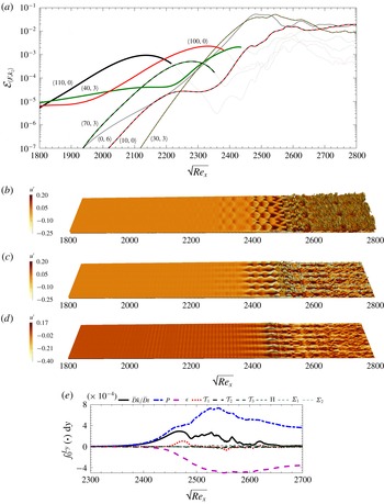
Results corresponding to case E1N. (a) Fluctuation energy content for selected instability modes, ${\mathcal{E}}_{\langle F,k_{z}\rangle }$ , versus the streamwise coordinate. Frequency $F$ is the normalized frequency and $k_{z}$ is the integer spanwise wavenumber, defined in (3.1) and (3.2). (b–d) Instantaneous iso-surfaces of streamwise velocity component, (b) $u=0.9$ , (c)  $u=0.6$ and (d)  $u=0.3$ , coloured by the streamwise velocity fluctuations $u^{\prime }$ . (e) The TKE transport terms integrated in the wall-normal direction along the transition zone.

The downstream development of ${\mathcal{E}}_{\langle F,k_{z}\rangle }$ of modes that play a principal role in transition was evaluated using (4.2) and is plotted in figures 9 and 11. For clarity, the curves become thin and faintly coloured beyond the location where their interactions are discussed. Figures 9 and 11 also include instantaneous iso-surfaces of streamwise velocity $u$ coloured by its fluctuation $u^{\prime }$ . Figures 9(e) and 11(e) feature the downstream development of integrated terms of the TKE equation

(4.3) $$\begin{eqnarray}\displaystyle \underbrace{\frac{1}{2}{\displaystyle \frac{\unicode[STIX]{x2202}\overline{\unicode[STIX]{x1D70C}u_{i}^{\prime \prime }u_{i}^{\prime \prime }}}{\unicode[STIX]{x2202}t}}+\frac{1}{2}{\displaystyle \frac{\unicode[STIX]{x2202}\overline{u_{j}}^{f}\overline{\unicode[STIX]{x1D70C}u_{i}^{\prime \prime }u_{i}^{\prime \prime }}}{\unicode[STIX]{x2202}x_{j}}}}_{\bar{D}k/\bar{D}t} & = & \displaystyle \underbrace{-\overline{\unicode[STIX]{x1D70C}u_{i}^{\prime \prime }u_{j}^{\prime \prime }}{\displaystyle \frac{\unicode[STIX]{x2202}\overline{u_{i}}^{f}}{\unicode[STIX]{x2202}x_{j}}}}_{P}\underbrace{-\overline{\unicode[STIX]{x1D70F}_{ij}^{\prime }{\displaystyle \frac{\unicode[STIX]{x2202}u_{i}^{\prime \prime }}{\unicode[STIX]{x2202}x_{j}}}}}_{\unicode[STIX]{x1D716}}\underbrace{-{\displaystyle \frac{1}{2}}\frac{\unicode[STIX]{x2202}\overline{\unicode[STIX]{x1D70C}u_{i}^{\prime \prime }u_{i}^{\prime \prime }u_{j}^{\prime \prime }}}{\unicode[STIX]{x2202}x_{j}}}_{{\mathcal{T}}_{1}}\nonumber\\ \displaystyle & & \displaystyle \underbrace{-{\displaystyle \frac{\unicode[STIX]{x2202}\overline{p^{\prime }u_{i}^{\prime }\unicode[STIX]{x1D6FF}_{ij}}}{\unicode[STIX]{x2202}x_{j}}}}_{{\mathcal{T}}_{2}}+\underbrace{{\displaystyle \frac{\unicode[STIX]{x2202}\overline{\unicode[STIX]{x1D70F}_{ij}^{\prime }u_{i}^{\prime \prime }}}{\unicode[STIX]{x2202}x_{j}}}}_{{\mathcal{T}}_{3}}+\underbrace{\overline{p^{\prime }{\displaystyle \frac{\unicode[STIX]{x2202}u_{i}^{\prime \prime }}{\unicode[STIX]{x2202}x_{i}}}}}_{\unicode[STIX]{x1D6F1}}+\underbrace{\overline{u_{i}^{\prime \prime }}{\displaystyle \frac{\unicode[STIX]{x2202}\overline{\unicode[STIX]{x1D70F}_{ij}}}{\unicode[STIX]{x2202}x_{j}}}}_{\unicode[STIX]{x1D6F4}_{1}}\underbrace{-\overline{u_{i}^{\prime \prime }}{\displaystyle \frac{\unicode[STIX]{x2202}\overline{p}}{\unicode[STIX]{x2202}x_{i}}}}_{\unicode[STIX]{x1D6F4}_{2}}.\end{eqnarray}$$

For an arbitrary quantity ${\mathcal{X}}$ , the Reynolds average is denoted by $\overline{{\mathcal{X}}}$ , the Favre (density-weighted) average is identified by $\overline{{\mathcal{X}}}^{f}$ and fluctuations with respect to the Reynolds and Favre averages are represented as ${\mathcal{X}}^{\prime }$ and ${\mathcal{X}}^{\prime \prime }$ , respectively. The terms on the right-hand side of (4.3) correspond to production rate $P$ , dissipation rate $\unicode[STIX]{x1D716}$ , transport by velocity fluctuations ${\mathcal{T}}_{1}$ , transport by pressure fluctuation ${\mathcal{T}}_{2}$ , transport by viscous diffusion ${\mathcal{T}}_{3}$ , pressure dilatation (pressure–strain) $\unicode[STIX]{x1D6F1}$ , viscous mass flux coupling $\unicode[STIX]{x1D6F4}_{1}$ and pressure mass flux coupling $\unicode[STIX]{x1D6F4}_{2}$ .

In case E1N, transition involves a series of instability waves that are activated at various downstream locations (figure 9 a): the inflow modes amplify first and, downstream, spur other instabilities which were not prominently featured in the inlet condition. Specifically, the inlet pair $\langle 100,0\rangle$ and $\langle 110,0\rangle$ activate mode $\langle 10,0\rangle$ – an interaction that we will denote ${\mathcal{I}}^{(1)}$ . The resulting mode $\langle 10,0\rangle$ is manifest as a low-frequency modulation of the near-wall waves in figure 9(d). In a subsequent interaction ${\mathcal{I}}^{(2)}$ , the pair $\langle 40,3\rangle$ and $\langle 110,0\rangle$ give rise to mode $\langle 70,3\rangle$ , which is visible in figure 9(b) near $\sqrt{Re_{x}}=2300$ . The next interaction ${\mathcal{I}}^{(3)}$ involves the newly formed three-dimensional mode and the inflow wave $\langle 100,0\rangle$ . It spurs the instability $\langle 30,3\rangle$ which grows at the highest rate, as evident in figure 9(b) in the range $2400<\sqrt{Re_{x}}<2550$ , and is the seat of breakdown to turbulence (also see supplementary movie 1). Note that a triad ${\mathcal{I}}^{(4)}$ is established between the first two nonlinearly generated waves, $\langle 10,0\rangle$ and $\langle 40,3\rangle$ , and the fastest amplifying instability $\langle 30,3\rangle$ . Flow structures resembling interweaving rope-shaped waves evolve far from the wall prior to breakdown to turbulence in supplementary movie 1, and bear resemblance to those observed experimentally in second-mode transition at Mach 5–8 (Casper et al. Reference Casper, Beresh, Henfling, Spillers, Pruett and Schneider2016; Laurence et al. Reference Laurence, Wagner and Hannemann2016).

Streaks feature in the instantaneous field (figures 9 c,d). In the spectra, they correspond to mode $\langle 0,6\rangle$ , which can be generated by the nonlinear interaction of modes $\langle \pm F,3\rangle$ ; their spanwise size is approximately equal to the thickness of the boundary layer at $\sqrt{Re_{x}}\approx 2600$ . The energy of the streaks, or mode $\langle 0,6\rangle$ , shadows that of mode $\langle 30,3\rangle$ which was discussed in connection with the outer $\unicode[STIX]{x1D6EC}$ -shaped structure and breakdown to turbulence. The breakdown of the streaks follows almost immediately after that of the outer $\unicode[STIX]{x1D6EC}$ shapes.

The interactions ${\mathcal{I}}$ described above can only be hypothesized based on the spectra. For example, whether the streaks $\langle 0,6\rangle$ are due to the self interactions of $\langle \pm 30,3\rangle$ , $\langle \pm 40,3\rangle$ or $\langle \pm 70,3\rangle$ cannot be conclusively determined; the similarity between $\langle \pm 30,3\rangle$ and $\langle \pm 0,6\rangle$ suggests a connection but does not guarantee it. In order to quantify the nonlinear interactions, we compute the energy transfer terms among wavenumber triads. Starting from ${\mathcal{T}}_{1}$ in (4.3), the following expression for ${\mathcal{I}}$ can be derived (see appendix B for details):

(4.4) $$\begin{eqnarray}\displaystyle {\mathcal{I}}_{\langle F,k_{z}\rangle }=\mathop{\sum }_{\pm F,\pm k_{z}}\int _{0}^{L_{y}}|\hat{\boldsymbol{{\mathcal{A}}}}_{\langle F_{1},k_{z,1}\rangle }^{\ast }\hat{\boldsymbol{{\mathcal{B}}}}_{\langle F_{2},k_{z,2}\rangle }+\hat{\boldsymbol{{\mathcal{A}}}}_{\langle -F_{2},-k_{z,2}\rangle }^{\ast }\hat{\boldsymbol{{\mathcal{B}}}}_{\langle -F_{1},-k_{z,1}\rangle }|\,\text{d}y, & & \displaystyle\end{eqnarray}$$

where $F=F_{2}-F_{1}$ and $k_{z}=k_{z,2}-k_{z,1}$ . In equation (4.4), $\hat{\boldsymbol{{\mathcal{A}}}}$ and $\hat{\boldsymbol{{\mathcal{B}}}}$ are vector quantities containing the Fourier coefficients of $\boldsymbol{{\mathcal{A}}}=\left[\begin{array}{@{}ccc@{}}\unicode[STIX]{x1D70C}u^{\prime \prime }u^{\prime \prime } & \unicode[STIX]{x1D70C}u^{\prime \prime }v^{\prime \prime } & \unicode[STIX]{x1D70C}u^{\prime \prime }w^{\prime \prime }\end{array}\right]^{\mathit{tr}}$ and of $\boldsymbol{{\mathcal{B}}}=\left[\begin{array}{@{}ccc@{}}u^{\prime \prime } & v^{\prime \prime } & w^{\prime \prime }\end{array}\right]^{\mathit{tr}}.$ The quantity ${\mathcal{I}}_{\langle F,k_{z}\rangle }$ thus represents the nonlinear energy transfer among modes $\langle F,k_{z}\rangle$ , $\langle F_{1},k_{z,1}\rangle$ and $\langle F_{2},k_{z,2}\rangle$ (Cheung & Zaki Reference Cheung and Zaki2010). Since ${\mathcal{I}}_{\langle F,k_{z}\rangle }$ is independent of the ordering of modes within the triad, it only measures the energy transfer among the three modes but not the direction of the transfer.

In case E1N, nonlinear interactions feature prominently and, therefore, ${\mathcal{I}}_{\langle F,k_{z}\rangle }$ for the seven most important interactions is plotted in figure 10. Note that the designation $\langle F_{1},k_{z,1}\rangle +\langle F_{2},k_{z,2}\rangle \Rightarrow \langle F,k_{z}\rangle$ in the figure is only intended to identify the triad, and bears no physical significance. However, together with the energy spectra, ${\mathcal{I}}_{\langle F,k_{z}\rangle }$ can provide a clearer view of the nonlinear interactions that spur new instability waves. The interaction ${\mathcal{I}}^{(1)}$ takes place between inflow modes $\langle 100,0\rangle$ and $\langle 110,0\rangle$ and generates $\langle 10,0\rangle$ . Similarly, ${\mathcal{I}}^{(2)}$ takes place between inlet modes $\langle 40,3\rangle$ and $\langle 110,0\rangle$ and gives rise to $\langle 70,3\rangle$ . This emergent mode has a strong interaction ${\mathcal{I}}^{(3)}$ with $\langle 100,0\rangle$ and leads to $\langle 30,3\rangle$ which amplifies at the highest rate. Note also that near $\sqrt{Re_{x}}\approx 2300$ , this interaction is overtaken by another triad, ${\mathcal{I}}^{(4)}$ , that involves $\langle 30,3\rangle$ . The source of the streaks $\langle 0,6\rangle$ is not a single interaction, but rather three, ${\mathcal{I}}^{(5,6,7)}$ , and each of them is dominant over a different region in the streamwise direction: ${\mathcal{I}}^{(5)}$ initiates the streaks in the region $\sqrt{Re_{x}}<2150$ ; ${\mathcal{I}}^{(6)}$ takes over in the range $2150<\sqrt{Re_{x}}<2270$ ; and finally the interaction ${\mathcal{I}}^{(7)}$ is dominant beyond $\sqrt{Re_{x}}\approx 2270$ , where the streaks become visible in the instantaneous visualizations (figure 9 c,d), and where mode $\langle 0,6\rangle$ shadows $\langle 30,3\rangle$ in the spectra.

The role of every interaction, including those that precede the amplification of $\langle 30,3\rangle$ , cannot be discounted. We performed exhaustive tests that involved assigning a significant portion of the inflow energy to mode $\langle 30,3\rangle$ but transition was delayed. Thus, all the events, including nonlinear interactions and base-flow distortion, that precede the formation of this mode must take place for transition to set in as upstream as recorded in our simulations.

Figure 10.

The modal nonlinear energy transfer coefficient, defined in (4.4), computed for the most important modal interactions corresponding to transition scenario of case E1N.

Terms in the TKE equation are shown versus downstream Reynolds number in figure 9(e). Three regions can be distinguished, based on the behaviour of the rate of production $P$ , which represents the energy exchange between the base state and the instability waves. (i) In the range $2400<\sqrt{Re_{x}}<2500$ , the production increases faster than dissipation; in this region, the instability wave $\langle 30,3\rangle$ dominates the spectra and reaches saturation. (ii) In the region $2500<\sqrt{Re_{x}}<2550$ , the rate of production increases as the secondary instability sets in and leads to the formation of the $\unicode[STIX]{x1D6EC}$ -structures and their local breakdown. (iii) Finally, in the range $2550<\sqrt{Re_{x}}<2650$ , the flow starts to approach the statistical state of a self-similar turbulent boundary layer.

Figure 11.

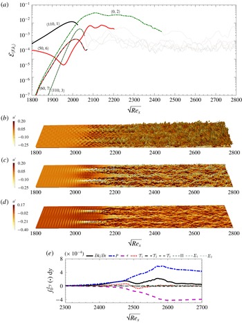
Results corresponding to case E2N. (a) Fluctuation energy content for selected instability modes, ${\mathcal{E}}_{\langle F,k_{z}\rangle }$ , versus the streamwise coordinate. Frequency $F$ is the normalized frequency and $k_{z}$ is the integer spanwise wavenumber, defined in (3.1) and (3.2). (b–d) Instantaneous iso-surfaces of streamwise velocity component, (b) $u=0.9$ , (c) $u=0.6$ and (d) $u=0.3$ , coloured by the streamwise velocity fluctuations $u^{\prime }$ . (e) The TKE transport terms integrated in the wall-normal direction along the transition zone.

The transition scenario for case E2N is of different ilk. Figure 11(a) captures the fast emergence and amplification of a streamwise elongated streak mode $\langle 0,2\rangle$ . This wave becomes the seat of secondary instability and onset of turbulence. Its instantaneous form is evident in the visualization of the streamwise velocity iso-surfaces (figure 11 b–d). The spanwise size of the structure is nearly three times the boundary-layer thickness at $\sqrt{Re_{x}}\approx 2250$ , which is the approximate location where the flow has reached a self-similar turbulent state. Streaks with commensurate sizes were reported in transition at $Ma_{\infty }=3$ (Mayer et al. Reference Mayer, Von Terzi and Fasel2011) and also at $Ma_{\infty }=6$ (Franko & Lele Reference Franko and Lele2013).

The streak $\langle 0,2\rangle$ is generated by modes $\langle \pm 110,1\rangle$ , which initially amplify linearly and peak near $\sqrt{Re_{x}}\approx 2000$ (cf. figure 11 a) – the location where the skin-friction coefficient starts to rise (cf. figure 3 b). At this stage, the mode $\langle 50,6\rangle$ starts to amplify, and reaches its highest energy level at $\sqrt{Re_{x}}\approx 2100$ . In the instantaneous realization, it appears to affect the secondary instability of the streak mode $\langle 0,2\rangle$ , which meanders and breaks down to turbulence (figure 11 b–d and supplementary movie 2). This interpretation was verified by examining the spectra and nonlinear energy transfer terms (not shown here); we have also performed numerous linear parabolized stability equation studies of the evolution of instability waves atop the Blasius similarity profile and also the mean-flow profile from case E2N.

Despite describing case E2N as a second-mode oblique transition, it is not without differences from the typical configuration where nearly all the disturbance energy is assigned to the oblique mode and a very small amount is included in broadband noise. For E2N, high levels of energy are included in both modes $\langle 110,1\rangle$ and $\langle 50,6\rangle$ at the inlet. As a result, their nonlinear interaction is active early upstream and generates mode $\langle 60,7\rangle$ (figure 11 a). This and other spurred oblique waves, e.g.  $\langle 110,3\rangle$ , promote breakdown of the streaky boundary layer to turbulence.

The upstream stages of transition in supplementary movie 2 exhibit alternation of light and dark regions within the bulk of the boundary layer. These regions amplify downstream and ultimately break down into turbulence. While rope-like structures appear near the boundary-layer edge close to transition onset, they do not undergo the spatial growth observed in case E1N. The qualitative change in transition at different levels of disturbance energy is important. A parallel, although not a one-to-one correspondence, can be drawn to the qualitative changes observed in the recent experiments of transition on a slender $7^{\circ }$ half-angle cone at Mach 6–7, conducted at low- and high-enthalpy conditions (Laurence et al. Reference Laurence, Wagner and Hannemann2016).

We can further examine the transition zone of case E2N by considering the evolution of terms in the TKE equation in various subregions (figure 11 e). In a similar manner to the discussion of case E1N, three regions can be identified. (i) In the range $2000<\sqrt{Re_{x}}<2100$ , the increase in the rate of production, $P$ , is moderate but $P$ itself exceeds the integrated $\unicode[STIX]{x1D716}$ . The energy of the streaks overtakes all other modes at the start of this region, and their secondary instability is amplifying. (ii) In the region $2100<\sqrt{Re_{x}}<2200$ , the secondary instability $\langle 50,6\rangle$ is nearly saturated (cf. figure 11 a), and localized patches of turbulence emerge; here the increases in the rate of production and dissipation become steeper, the latter enhanced by the emergence of small turbulent scales. Within the localized patches of turbulence, production exceeds the levels of fully turbulent boundary layers (Marxen & Zaki Reference Marxen and Zaki2019). (iii) In the region $2200<\sqrt{Re_{x}}<2300$ , the turbulence spread and fills the domain, and terms in the TKE equation start to relax towards their equilibrium values for self-similar turbulent boundary layers.

Figure 12.

Wall-normal profiles of time- and spanwise-averaged streamwise velocity $\bar{u}$ (a,b) and temperature $\overline{T}$ (c,d) at different locations along the transition zone. (a,c) The profiles of case E1N correspond to $2400\leqslant \sqrt{Re_{x}}\leqslant 2700$ with increment of $50$ from light to dark colours (also thin to thick lines). (b,d) The profiles of case E2N correspond to $2000\leqslant \sqrt{Re_{x}}\leqslant 2300$ with increment of $50$ from light to dark colours (also thin to thick lines).

Figure 13.

Iso-surfaces of $Q=1\times 10^{-4}$ coloured by $u^{\prime }$ (a,b) and $v^{\prime }$  (c,d) corresponding to cases (a,c) E1N and (b,d) E2N.

The transition processes in cases E1N and E2N are contrasted in figures 12 and 13. The former figure shows wall-normal profiles of the mean streamwise velocity and temperature, evaluated at different streamwise positions within the transition zone. And the latter figure shows three-dimensional views of the vortical structures, visualized using the $Q$ -criterion, within the transition regions of both cases. Transition in case E1N takes place via the formation and breakdown of $\unicode[STIX]{x1D6EC}$ -shaped vortices. This process takes place over a relatively short streamwise distance as shown qualitatively in figure 13 and demonstrated by the skin-friction coefficient along the plate (figure 3). The relatively abrupt transition is accompanied by a distortion of the mean streamwise velocity profile in the near-wall region, followed by a subsequent relaxation of the outer part of the profile towards the fully turbulent curve. The same trend is captured in the mean temperature profile. In case E2N, transition is due to the secondary instability of streamwise-elongated streaks. While the streaks themselves are not captured in the visualization of the $Q$ -criterion, their secondary instability is seen in figure 13(b,d). The transition length is longer in this case, and therefore the mean velocity and temperature profiles gradually approach the turbulent curve.

For case E1N, figure 13(a,c) shows that the $\unicode[STIX]{x1D6EC}$ -structures, which are generated as a result of the amplification of mode $\langle 30,3\rangle$ , are located close to the edge of the boundary layer. They lie above the near-wall streaks shown in figure 9(d), and successive rows of $\unicode[STIX]{x1D6EC}$ -structures are staggered in the spanwise direction. Typical of hairpin structures in wall-bounded flows (see e.g. Adrian Reference Adrian2007; Farano et al. Reference Farano, Cherubini, Robinet and De Palma2015), their legs lead to ejections in the plane of symmetry while the head generates a strong sweep motion. The wall-normal and streamwise velocity fluctuations therefore have opposite signs in those regions. Ejections due to positive wall-normal velocity fluctuations are accompanied by transport of low streamwise momentum upward and a negative streamwise fluctuation; sweep due to negative $v^{\prime }$ leads to downward transport of high-momentum fluid and a positive $u^{\prime }$ perturbation. The late stages in the evolution of these $\unicode[STIX]{x1D6EC}$ -structures resemble natural transition to turbulence, where trains of hairpin vortices are formed and break down over a short streamwise distance. Since the structures are staggered in the span, a fully turbulent flow is established quickly downstream thus leading to a short transition length.

Figure 13(b,d) for case E2N shows that $\unicode[STIX]{x1D6EC}$ -structures form in this case as well, and successive rows are similarly staggered in the spanwise direction. However, breakdown to turbulence does not commence at the tips of individual structures; instead it is initiated due to the instability of the underlying steady streaks. These streaks are clearly captured in figure 11(d), and at the same locations the breakdown pattern is clear in figure 13(b,d). In this region, the streaks are elevated low-speed structures (negative $u^{\prime }$ ) straddled by $\unicode[STIX]{x1D6EC}$ -structures that induce their ejection (positive $v^{\prime }$ ). Since breakdown takes place on the low-speed streaks, it directly impacts every other row of the $\unicode[STIX]{x1D6EC}$ -structures and subsequently spreads to fill the domain; the transition length is therefore longer in this case relative to E1N.

4.3 Prediction from linear stability theory

In order to highlight the importance of the present nonlinear approach in determining the inflow disturbance spectrum, we examine other possible inflow conditions that are selected based on linear theory alone. The starting point is to evaluate the linear evolution of all the Orr–Sommerfeld and Squire instability waves that are part of the inlet condition, using the linear parabolized instability equations (Park & Zaki Reference Park and Zaki2019). The $N$ -factor associated with every $\langle F,k_{z}\rangle$ wave was obtained as follows:

(4.5) $$\begin{eqnarray}\displaystyle N\text{-factor}=\frac{1}{2}\ln \left({\displaystyle \frac{{\mathcal{E}}_{\langle F,k_{z}\rangle }}{{\mathcal{E}}_{0}}}\right), & & \displaystyle\end{eqnarray}$$

where ${\mathcal{E}}_{0}$ is the energy of the mode at the inlet. The results are shown for three downstream locations in figure 14(a). Depending on the point at which the growth rates are computed, different instability waves attain the highest $N$ -factor value. Figure 14(b) shows the change of $N$ -factor versus streamwise location for the four instability waves that are each most amplified within a subregion of the computational domain: mode $\langle 110,0\rangle$ for $\sqrt{Re_{x}}<2190$ , mode $\langle 100,0\rangle$ along $2190<\sqrt{Re_{x}}<2470$ , mode $\langle 90,0\rangle$ along $2470<\sqrt{Re_{x}}<2650$ and mode $\langle 20,2\rangle$ for $\sqrt{Re_{x}}>2650$ . In order to make use of these results in selecting the inflow condition, prior knowledge of the transition location is needed; linear theory does not provide this information.

Figure 14.

(a) Contours of $N$ -factor computed from (4.5) from left to right for $\sqrt{Re_{x_{f}}}=2100$ , $2500$ and $2900$ , respectively. (b) The $N$ -factor of the important modes versus streamwise location. (c) Skin friction curves corresponding to the nonlinearly most dangerous cases (E1N and E2N) and the linearly most unstable cases (E1L1, E1L2, E1L3 and E2L) presented in table 2.

We examined four inflow conditions that were selected based on the linear results, and computed their evolution using direct numerical simulations in order to compare the outcome to the nonlinearly most dangerous disturbance. These new cases are designated E1L1, E1L2, E1L3 and E2L, and their parameters are reported in table 2. The first three are at the lower inflow energy level and, since transition is expected in the second half of the domain, 99 % of the inflow energy is allocated to modes $\langle 100,0\rangle$ , $\langle 90,0\rangle$ and $\langle 20,2\rangle$ , respectively. The fourth case, E2L, is at the higher inflow energy level and, therefore, 99 % of the inflow energy is assigned to mode $\langle 110,0\rangle$ . For all four cases, the remaining 1 % of the inflow energy was in the form of broadband forcing, in order to enable possible nonlinear interactions and secondary instabilities. The outcome of these simulations is contrasted to the nonlinearly most dangerous cases in figure 14(c), where $C_{f}$ is plotted versus downstream distance. Note that, for some of these simulations, the domain was extended in the streamwise direction in order to capture the delayed transition to turbulence, in particular in E1L1 and E1L2.

The transition scenarios in the new simulations are very different from those due to the nonlinearly optimal inflow conditions. The streamwise development of the energy of associated key modes is reported in figure 2 of the supplementary material. Cases E1L1 and E1L2 are akin to classical two-dimensional second-mode transition, with a region of oblique secondary instability prior to breakdown. Case E1L3 is a typical first-mode oblique breakdown, in which the primary three-dimensional wave develops oblique instabilities, $\unicode[STIX]{x1D6EC}$ -structures and ultimately hairpin vortices that become the seat for the onset of turbulence. Transition in case E2L is a typical second-mode fundamental scenario, where the oblique secondary instability has the same frequency as the primary two-dimensional wave.

In all four cases, the inflow primary instability is the key determinant of the path to turbulence. And while the linearly most unstable waves guarantee fastest exponential growth based on linear theory, they do not necessarily guarantee largest energy in the nonlinear regime or earliest secondary instability and transition. In contrast, when the nonlinearly most dangerous inflow condition was adopted, the resulting transition mechanism was not due to any one particular inflow wave; instead, the nonlinear interactions of the inflow instabilities led to the generation of new waves, the distortion of the base flow and the earliest possible transition location.