



1 Introduction
Computably enumerable (c.e.) degrees are fundamental objects in both classical and reverse recursion theory. The Friedberg–Muchnik Theorem [Reference Friedberg6, Reference Muchnik11] and the Sacks Splitting Theorem [Reference Sacks16] are two important results for the c.e. degrees, proved by finite-injury priority arguments. From the viewpoint of injury bounds, the Sacks Splitting Theorem differs from the Friedberg–Muchnik Theorem. If the number of injuries can be effectively bounded, the argument is of bounded type; otherwise, it is of unbounded type. In this sense, the Friedberg–Muchnik construction is of bounded type, while the Sacks Splitting construction is of unbounded type. This distinction is also confirmed in reverse recursion theory. Chong and Mourad [Reference Chong and Mourad2] proved that the Friedberg–Muchnik Theorem is provable in models of
$\mathsf {P}^-+\mathsf {I}\Sigma _0+\mathsf {B}\Sigma _1+\mathrm {Exp}$
 . By contrast, Mytilinaios [Reference Mytilinaios12] and Slaman and Woodin [Reference Slaman and Woodin19] showed that the Sacks Splitting Theorem is equivalent to
$\mathsf {I}\Sigma _1$
 over the base theory
$\mathsf {P}^-+\mathsf {I}\Sigma _0+\mathsf {B}\Sigma _1+\mathrm {Exp}$
 . We remark that it is not the case that bounded-type finite-injury arguments can always be carried out in models of
$\mathsf {P}^-+\mathsf {I}\Sigma _0+\mathsf {B}\Sigma _1+\mathrm {Exp}$
 ; Chong and Yang [Reference Chong and Yang4] showed that the existence of a noncomputable low c.e. degree is equivalent to
$\mathsf {I}\Sigma _1$
 over
$\mathsf {P}^-+\mathsf {I}\Sigma _0+\mathsf {B}\Sigma _1+\mathrm {Exp}$
 .
In [Reference Mytilinaios12], Mytilinaios exploited a blocking technique from
$\alpha $
 -recursion theory introduced by Shore [Reference Shore17], and proved the following theorem.
Theorem 1.1 (The Sacks Splitting Theorem [Reference Mytilinaios12, Reference Sacks16]).
The following holds in models of
$\mathsf {P}^-+\mathsf {I}\Sigma _1$
 : Let
$\boldsymbol {b}$
 be a c.e. degree. Then there exist incomparable c.e. degrees
$\boldsymbol {a_0}$
 and
$\boldsymbol {a_1}$
 such that
$\boldsymbol {b}= \boldsymbol {a_0}\vee \boldsymbol {a_1}$
 .
Robinson proved the following refinement of the Sacks Splitting Theorem.
Theorem 1.2 (The Robinson Splitting Theorem [Reference Robinson15]).
Let
$\boldsymbol {b}>\boldsymbol {c}$
 be c.e. degrees with
$\boldsymbol {c}$
 a low c.e. degree. Then there exist incomparable c.e. degrees
$\boldsymbol {a_0}$
 and
$\boldsymbol {a_1}$
 such that
$\boldsymbol {b}= \boldsymbol {a_0}\vee \boldsymbol {a_1}$
 with
$\boldsymbol {a_i}>\boldsymbol {c}$
 for
$i<2$
 .
Here, a set A is low if
$A'\le _T \varnothing '$
 ; that is, the jump of A has the least possible Turing degree. (Lachlan’s Nonsplitting Theorem [Reference Lachlan10] asserts that the above theorem is in general false if
$\boldsymbol {c}$
 is not low: more precisely, there exist c.e. degrees
$\boldsymbol {b}>\boldsymbol {c}$
 such that
$\boldsymbol {b}$
 does not split over
$\boldsymbol {c}$
 .) In the construction, Robinson introduced a method, now often referred to as Robinson’s trick, for approximating an answer computable from
$\boldsymbol {0}'$
 . This method allows only finitely many wrong guesses, which makes the construction possible. This introduces another finiteness issue, in addition to the finite-injury behavior in the Sacks Splitting Theorem. Can this additional finiteness be treated in models of
$\mathsf {I}\Sigma _1$
 ? Although it is often believed that finite-injury priority arguments can be carried out in models of
$\mathsf {I}\Sigma _1$
 , this is not immediate for the Robinson Splitting Theorem. We prove a weaker version of the Robinson Splitting Theorem in models of
$\mathsf {I}\Sigma _1$
 , replacing the lowness of
$\boldsymbol {c}$
 with super-lowness. Recall that a set C is super-low in classical recursion theory if
$C'\le _{wtt} \varnothing '$
 . The precise definitions of super-lowness in reverse recursion theory, as well as of other relevant notions such as c.e. sets, are given in Section 2.
Our main result is the following theorem.
Theorem 1.3. The following holds in models of
$\mathsf {P}^-+\mathsf {I}\Sigma _1$
 : Given c.e. degrees
$\boldsymbol {b},\boldsymbol {c},\boldsymbol {d}$
 with
$\boldsymbol {c}$
 super-low and
$\boldsymbol {d}\nleq \boldsymbol {c}$
 , there exist incomparable c.e. degrees
$\boldsymbol {a_0},\boldsymbol {a_1}$
 such that
$\boldsymbol {b}= \boldsymbol {a_0}\vee \boldsymbol {a_1}$
 with
$\boldsymbol {d}\nleq \boldsymbol {a_i}\vee \boldsymbol {c}$
 for
$i<2$
 .
Taking
$\boldsymbol {d}=\boldsymbol {b}>\boldsymbol {c}$
 recovers the Robinson Splitting Theorem.
Corollary 1.4. The following holds in models of
$\mathsf {P}^-+\mathsf {I}\Sigma _1$
 : Let
$\boldsymbol {b}>\boldsymbol {c}$
 be c.e. degrees with
$\boldsymbol {c}$
 super-low. Then there exist incomparable c.e. degrees
$\boldsymbol {a_0},\boldsymbol {a_1}$
 such that
$\boldsymbol {b}= \boldsymbol {a_0}\vee \boldsymbol {a_1}$
 with
$\boldsymbol {a_i}>\boldsymbol {c}$
 for
$i<2$
 .
For Theorem 1.3 to be meaningful, we need
$\mathsf {P}^-+\mathsf {I}\Sigma _1$
 to prove the existence of a noncomputable super-low set. This is indeed the case: the standard construction of a noncomputable low set is a bounded-type finite-injury argument and therefore goes through in models of
$\mathsf {P}^-+\mathsf {I}\Sigma _1$
 . Moreover, since the number of injuries is effectively bounded, the set obtained is automatically
$\omega $
 -c.e. and hence super-low (see Lemma 2.18).
In Section 2, we recall the basic setting of reverse recursion theory and the inductive hierarchy (for further background, see Chong, Li, and Yang [Reference Chong, Li and Yang1]). The formal definitions of c.e. sets and the reducibilities used for c.e. degrees are given there. In Section 3, we present a proof of the Sacks Splitting Theorem in models of
$\mathsf {P}^-+\mathsf {I}\Sigma _1$
 . The reader may also consult the original paper of Mytilinaios [Reference Mytilinaios12]; our presentation differs slightly from the original one. Building on this framework, we make the necessary modifications in Section 4 to prove our main result (Theorem 1.3). More precisely, the ideas of blocking and dynamic priority assignments remain the same. The main difficulty lies in the proof of Lemma 4.5, which is the analogue of Lemma 3.2.
2 Preliminaries
In this section, we recall the basic concepts from reverse recursion theory and classical recursion theory that lead to Corollary 2.19, a key ingredient in the proof of Theorem 1.3.
We work in the language of arithmetic
$\mathcal {L}=\{0,+,\times ,<,\exp \}$
 and the base theory
$\mathsf {P}^-+\mathsf {I}\Sigma _1$
 . Here
$\mathsf {P}^-$
 denotes the axioms of
$\mathsf {PA}$
 with the induction scheme omitted. Also,
$\mathsf {I}\Sigma _n$
 (resp.
$\mathsf {I}\Pi _n$
 ) denotes the induction scheme for
$\Sigma _n$
 (resp.
$\Pi _n$
 ) formulas, and
$\mathsf {B}\Sigma _n$
 (resp.
$\mathsf {B}\Pi _n$
 ) denotes the collection scheme for
$\Sigma _n$
 (resp.
$\Pi _n$
 ) formulas.
$\mathsf {L}\Sigma _1$
 (resp.
$\mathsf {L}\Pi _1$
 ) denotes the assertion that every nonempty
$\Sigma _1$
 (resp.
$\Pi _1$
 ) subset has a least element. Finally,
$\mathrm {Exp}$
 denotes the axiom
$\forall x \exists y\,(y=\exp (x))$
 , where
$\exp :x\mapsto 2^x$
 is the exponential function. Some of the lemmas in this section are well known or straightforward; we include their proofs for completeness.
It is well known that:
Theorem 2.1 (Paris and Kirby [Reference Paris and Kirby14]).
Work in
$\mathsf {P}^-+\mathsf {I}\Sigma _0$
 . For all
$n \geq 0$
 ,
-
(1) $\mathsf {I}\Sigma _1\iff \mathsf {I}\Pi _1 \iff \mathsf {L}\Sigma _1 \iff \mathsf {L}\Pi _1$
 .
-
(2) $\mathsf {B}\Sigma _{n+1} \Leftrightarrow \mathsf {B}\Pi _n$
. -
(3) $\mathsf {I}\Sigma _{n+1} \Rightarrow \mathsf {B}\Sigma _{n+1} \Rightarrow \mathsf {I}\Sigma _n$
, and the implications are strict.



(Slaman [Reference Slaman18]) Work in
$\mathsf {P}^-+\mathsf {I}\Sigma _0+\mathrm {Exp}$
 . For all
$n\ge 1$
 ,
-
(4) $\mathsf {B}\Sigma _n\Leftrightarrow \mathsf {I}\Delta _n$
.

In Section 5, we will see that
$\mathsf {B}\Sigma _2$
 proves the original Robinson Splitting Theorem. Since
$\mathsf {B}\Sigma _2$
 is strictly stronger than
$\mathsf {I}\Sigma _1$
 , the proof of Theorem 1.3 requires additional care.
We now introduce the basic notions for the sets in our model. We adopt the standard pairing function, where the code of the pair
$(a,b)$
 under this function is denoted by
$\langle a, b\rangle $
 . Let M be a model of
$\mathsf {P}^- + \mathsf {I}\Sigma _0 + \mathrm {Exp}$
 . A subset
$A\subseteq M$
 is bounded if
$\exists b\in M\, \forall x\in A\, x<b$
 .
$A\subseteq M$
 is coded if there exists
$c\in M$
 such that
$x\in A$
 if and only if the x-th digit of the binary expansion of c is
$1$
 . A set
$A\subseteq M$
 is M-finite if it is coded by some
$c\in M$
 . In particular, an M-finite set is bounded in M.
Definition 2.2. A set
$A\subseteq M$
 is regular if, for each
$n\in M$
 , the restriction
$A \!\upharpoonright \! n := \{x\in A\mid x<n\}$
 is M-finite.
It is known that
$A\subseteq M$
 is regular if and only if
$M\models \mathsf {I}\Delta _0^A$
 . Here, a
$\Delta _0^A$
 -formula is a
$\Delta _0$
 -formula in the expanded language
$\mathcal {L}_A=\{0,+,\times ,<,\exp ,A\}$
 , where we have an additional unary predicate
$A(x)$
 . To see why the equivalence holds:
$(\Rightarrow )$
 suppose there is a
$\Delta _0^A$
 -cut I defined by
$\varphi (x)\in \mathcal {L_A}$
 and a number
$b\notin I$
 . Then
$x\in I$
 if and only if
$x<b\land \varphi (x)$
 . But the latter formula depends only on a bounded part of the oracle A, and regularity turns the formula into a
$\Delta _0$
 formula, and hence the cut into a
$\Delta _0$
 -definable cut.
$(\Leftarrow )$
 “
$A\!\upharpoonright \! n$
 is coded” is a
$\Delta _0^A$
 formula, and
$\Delta _0^A$
 -induction yields regularity of A. For further details on the relevant normal-form argument, see Kleene [Reference Kleene9].
Definition 2.3. A set
$A\subseteq M$
 is hyperregular if
$M\models \mathsf {I}\Sigma _1^A$
 .
Here, a
$\Sigma _1^A$
 -formula is a
$\Sigma _1$
 -formula in the expanded language
$\mathcal {L}_A$
 . From the definition, since every
$\Delta _0^A$
 -formula is also a
$\Sigma _1^A$
 -formula, every hyperregular set is regular.
Next, we introduce the computability-theoretic notions in our model, so that we can discuss which kinds of sets are regular or hyperregular and which of their properties can be used in our proof. In the following, we use
$\bar {A}=M\setminus A$
 to denote the complement of A.
Definition 2.4.
-
(1) A set $A\subseteq M$
is c.e. if it is
$\Sigma _1$
definable (with parameters from M) in M. -
(2) A set $A\subseteq M$
is computable if A and
$\bar {A}$
are both c.e. -
(3) A function f is partial computable if its graph $G_f=\{\langle x,y\rangle \mid f(x)=y\}$
is c.e. -
(4) A function f is computable if it is partial computable and its domain equals M, that is, $\operatorname {\mathrm {dom}} f=\{x\in M\mid \exists y\in M, f(x)=y\}=M$
.


Note that if a function f is computable, then its graph
$G_f\subseteq M$
 is computable in the sense that
$G_f$
 and
$\bar {G_f}$
 are both c.e. However, the computability of
$G_f$
 alone only implies that f is partial computable.
Let us turn to Turing functionals and reducibility.
Definition 2.5.
-
(1) A Turing functional is a c.e. set $\Phi $
of axioms
$\langle x, y, P, N \rangle $
, where x and y are numbers,
$P, N$
are M-finite sets, and-
(a) $\langle x, y, P, N \rangle \in \Phi \rightarrow P \cap N =\emptyset $
, -
(b) $( \langle x, y, P, N \rangle \in \Phi \wedge P' \cap N' = \emptyset \wedge P \subseteq P' \wedge N \subseteq N') \rightarrow \langle x, y, P', N' \rangle \in \Phi $
, where
$P'$
and
$N'$
are M-finite sets, -
(c) $(\langle x, y, P, N \rangle , \langle x, y', P, N \rangle \in \Phi ) \rightarrow y = y'$
.
-
-
(2) Let $\{\Phi _e\mid e\in M\}$
be a fixed enumeration of all Turing functionals. -
(3) Let $B\subseteq M$
, and let
$\Phi $
be a Turing functional. We write
$\Phi ^B(x)=y$
if
$\langle x, y, P, N \rangle \in \Phi $
for some M-finite sets
$P\subseteq B$
and
$N\subseteq \bar {B}$
. We say
$\Phi ^B(x)$
converges, denoted by
$\Phi ^B(x)\downarrow $
, if for some y,
$\Phi ^B(x)=y$
. We let $$\begin{align*}W^B = \operatorname{\mathrm{dom}} \Phi^B = \{x\in M\mid \Phi^B(x)\downarrow\}. \end{align*}$$This is a $\Sigma _1^B$
set.
$\{W_e^B\mid e\in M\}$
lists all
$\Sigma _1^B$
sets. Let $$\begin{align*}B'=\{\langle e,x \rangle\mid x\in W_e^B\} \end{align*}$$be the jump of B. By convention, we let K denote $\varnothing '$
, the jump of the empty set.
-
(4) $A\subseteq M$
is B-computable if both A and
$\bar {A}$
are
$\Sigma _1^B$
. -
(5) Let $A, B \subseteq M$
. A is pointwise Turing reducible to B, denoted by
$A \leq _{pT} B$
, if there is a Turing functional
$\Phi $
such that
$A=\Phi ^B$
. That is, for all
$x\in M$
,
$A(x)=\Phi ^B(x)$
. -
(6) Let $A, B\subseteq M$
. A is strong Turing reducible to B, denoted by
$A \leq _{sT} B$
, if the sets $$ \begin{align*} &A^+=\{X\mid X \text{ is an } M\text{-finite subset of } A\}\\ &A^-=\{Y\mid Y \text{ is an } M\text{-finite subset of } \bar{A}\} \end{align*} $$are pointwise Turing reducible to B.
-
(7) A Turing degree is the equivalence class induced by $\le _{sT}$
.





It should be noted that for
$A\subseteq M$
 , being computable (in the sense that both A and
$\bar {A}$
 are c.e.) is equivalent to
$A\le _{pT}\varnothing $
 , and that being B-computable is equivalent to
$A\le _{pT} B$
 . It is clear that
$A\le _{sT} B$
 implies
$A\le _{pT} B$
 by definition. The difference between
$\le _{sT}$
 and
$\le _{pT}$
 is that the former is transitive (which justifies the term ‘Turing degree’ in Item (7) above), whereas Groszek and Slaman [Reference Groszek and Slaman7] showed that there is a model of
$\mathsf {P}^-+\mathsf {I}\Sigma _1$
 in which
$\le _{pT}$
 is not transitive on c.e. sets. In the same paper, it is shown in the following lemma.
Lemma 2.6 (Groszek and Slaman [Reference Groszek and Slaman7]).
Let M be a model of
$\mathsf {P}^-+\mathsf {I}\Sigma _0$
 . Suppose that Y is regular and
$M\models \mathsf {B}\Sigma _1^Y$
 and
$X\le _{pT} Y$
 . Then we have:
-
(1) $X\le _{sT} Y$
. -
(2) X is regular.
-
(3) $M\models \mathsf {B}\Sigma _1^X$
.


Corollary 2.7. Let M be a model of
$\mathsf {P}^-+\mathsf {I}\Sigma _1$
 . Suppose that Y is hyperregular. Then
$X\le _{pT} Y$
 if and only if
$X\le _{sT} Y$
 .
Proof. Since Y is hyperregular,
$M\models \mathsf {I}\Sigma _1^Y$
 . Therefore,
$M\models \mathsf {B}\Sigma _1^Y$
 . By Lemma 2.6, we have
$X\le _{sT} Y$
 if and only if
$X\le _{pT} Y$
 .
Definition 2.8. A function f is partial A-computable if its graph is
$\Sigma _1^A$
 ; and A-computable if it is partial A-computable and its domain
$\operatorname {\mathrm {dom}} f=M$
 .
If f is partial A-computable, then there exists some
$e\in M$
 such that

The following lemma is a well-known result.
Lemma 2.9 (H. Friedman).
Let M be a model of
$\mathsf {P}^-+\mathsf {I}\Sigma _1$
 .
-
(1) If $A\subseteq M$
is c.e., then A is regular. -
(2) Every partial computable function maps bounded subsets of M to bounded subsets of M.

Hyperregular sets can be characterized in several ways.
Lemma 2.10 (Mytilinaios and Slaman [Reference Mytilinaios and Slaman13]).
Let M be a model of
$\mathsf {P}^- + \mathsf {I}\Sigma _0 + \mathrm {Exp}$
 , and let
$A \subseteq M$
 be regular. Then the following are equivalent:
-
(1) A is hyperregular.
-
(2) Every partial A-computable function maps bounded subsets of M to bounded subsets of M.
-
(3) For all $e\in M$
,
$W_e^A$
is regular.


Recall that
$A\le _1 B$
 if there exists a computable function f such that for all
$x\in M$
 ,

For
$n\in M$
 , by
$\mathsf {B}\Sigma _1$
 , there exists b such that
$\forall x<n \left (f(x)<b\right )$
 . Suppose B is regular. Then
$B\!\upharpoonright \! b$
 is M-finite. For
$x<n$
 , we have
$x\in A \iff f(x)\in B\!\upharpoonright \! b$
 . This shows that A is also regular. Therefore, we have the following lemma.
Lemma 2.11. Let
$M\models \mathsf {P}^-+\mathsf {I}\Sigma _1$
 . If
$A\le _1 B$
 and B is regular, then A is regular.
Lemma 2.12. Let
$M\models \mathsf {P}^-+\mathsf {I}\Sigma _1$
 .
$C'$
 is regular if and only if C is hyperregular.
Proof.
$(\Rightarrow )$
 Note that
$C'$
 is
$\Sigma _1^C$
 -complete. That is, for all
$e\in M$
 ,
$W_e^C \le _1 C'$
 . In particular,
$C\le _1 C'$
 . Therefore, by Lemma 2.11, C and every
$W_e^C$
 are regular. By Lemma 2.10, C is hyperregular.
$(\Leftarrow )$
 By definition of hyperregularity, C is regular. For some
$e\in M$
 ,
$C'=W_e^C$
 . Since C is hyperregular,
$C'$
 is regular by Lemma 2.10(3).
Definition 2.13.
$A\subseteq M$
 is an
$\omega $
 -c.e. set if there exist computable functions f and g such that, for all
$x\in M$
 , we have
$f(x,s)=0$
 whenever
$x\ge s$
 ,
$A(x)=\lim _s f(x,s)$
 , and
$|\{s\mid f(x,s+1)\neq f(x,s)\}|\le g(x)$
 . Moreover, for
$n\in M$
 , A is an n-c.e. set if we can additionally require that
$g(x)=n$
 for all
$x\in M$
 .
We write
$x\in A_s$
 if
$f(x,s)=1$
 . Then
$\{A_s\}_{s\in M}$
 is called an approximation of A.
By this definition, A is c.e. if and only if A is
$1$
 -c.e. In this case, we may call
$\{A_s\}_{s\in M}$
 an enumeration of A, instead of an approximation of A. Also note that the set
$A_s$
 is bounded by s. The following property will be helpful in our construction.
Lemma 2.14. Let A be a c.e. set. Then A has an enumeration
$\{A_s\}_{s\in M}$
 such that, for each s, the set
$A_s\setminus A_{s-1}$
 is either empty or a singleton. Moreover, if s is even, then
$A_{s}\setminus A_{s-1}=\varnothing $
 .
Proof. Let
$\varphi $
 be a
$\Delta _0$
 -formula such that

For
$s\in M$
 , define

The sequence
$\{C_s\}_{s\in M}$
 is increasing with
$\bigcup _{s} C_s=A$
 . A number x enters
$C_s\setminus C_{s-1}$
 only if
$\langle x,y\rangle = s$
 for some
$y\le s$
 ; since the pairing function is injective, there is at most one such x, so
$C_s\setminus C_{s-1}$
 is empty or a singleton.
To make new elements appear only at odd stages, set
$A_{2s-1}=A_{2s}=C_s$
 . Then
$\{A_s\}_{s\in M}$
 is again an enumeration of A. At an even stage,
$A_{2s}\setminus A_{2s-1}=\varnothing $
 ; at an odd stage,
$A_{2s-1}\setminus A_{2s-2}=C_s\setminus C_{s-1}$
 is empty or a singleton. Hence
$\{A_s\}_{s\in M}$
 has the required properties.
Lemma 2.15. Let
$M\models \mathsf {P}^-+\mathsf {I}\Sigma _1$
 . Let
$A\subseteq M$
 be an
$\omega $
 -c.e. set. Then A is regular.
Proof. Let f and g be computable functions such that
$A(x)=\lim _s f(x,s)$
 and
$|\{s\mid f(x,s+1)\neq f(x,s)\}|\le g(x)$
 . Let C be the change set for f, i.e., enumerate
$\langle x,i-1\rangle $
 into C at stage s if
$f(x,s+1)\neq f(x,s)$
 for the i-th time. So C is c.e. and thus regular. For any
$n\in M$
 , let
$d=\max \{\, g(x)\mid x<n\}$
 , whose existence follows from
$\mathsf {I}\Sigma _1$
 . Let t code C up to
$\langle n, d\rangle $
 . Now,
$x\in A$
 if and only if
$|\{i\mid \langle x,i\rangle \in C\}|$
 is odd. So for any
$x<n$
 ,

Hence
$A\!\upharpoonright \! n$
 is coded in M for every
$n\in M$
 , so A is regular.
We now define super-low in models of
$\mathsf {P}^-+\mathsf {I}\Sigma _1$
 as in standard computability theory.
Definition 2.16.
-
(1) Let $\{\Phi _s\}_{s\in M}$
be an enumeration of the Turing functional
$\Phi $
. The use function
$\varphi ^B$
for
$\Phi ^B$
is a partial function
$\varphi ^B:M\to M$
such that
$\varphi ^B(x)\downarrow $
if and only if
$\Phi ^B(x)\downarrow $
. If
$\Phi ^B(x)\downarrow $
, we let s be the least s such that there exists a quadruple
$\langle x, y, P, N \rangle \in \Phi _s^B$
. Then
$\varphi ^B(x)=1+\max (P\cup N)$
. We adopt the convention that
$\varphi ^B, \psi ^B, \gamma ^B, \delta ^B$
denote use functions for
$\Phi ^B, \Psi ^B, \Gamma ^B, \Delta ^B$
, respectively. -
(2) We define $A\le _{wtt} B$
if
$A=\Phi ^B$
for some Turing functional
$\Phi $
and the use function
$\varphi ^B$
is bounded by a computable function. (Here, wtt stands for weak truth table.) A set
$A\subseteq M$
is super-low if
$A'\le _{wtt} K$
.





$A\le _{wtt} B$
 implies
$A\le _{pT} B$
 by definition.
Lemma 2.17. Let M be a model of
$\mathsf {P}^-+\mathsf {I}\Sigma _1$
 . Suppose B is regular and
$A\le _{wtt} B$
 . Then
$A\le _{sT} B$
 .
Proof. Suppose
$A=\Phi ^B$
 and its use function
$\varphi ^B$
 is bounded by f. Let F be an M-finite set. For each
$x\in F$
 , there exist M-finite sets
$P_x, N_x$
 such that
$\max P_x\cup N_x < f(x)$
 and

By
$\mathsf {B}\Sigma _1$
 , the range of f restricted to F is bounded by some b. Then, by the regularity of B,

are two M-finite sets so that for each
$x\in F$
 ,
$P_x\subseteq P$
 , and
$N_x\subseteq N$
 . Therefore, we have

Then we define
$\Psi $
 to be the c.e. set of all
$\langle F,i,P,N \rangle $
 such that

Then
$A^+=\Psi ^B$
 , which shows that
$A^+\le _{pT} B$
 . Similarly,
$A^-\le _{pT} B$
 . Hence,
$A\le _{sT} B$
 .
We also use the following characterization.
Lemma 2.18. Let
$M\models \mathsf {P}^-+\mathsf {I}\Sigma _1$
 .
$A\le _{wtt} K$
 if and only if A is
$\omega $
 -c.e.
Proof.
$(\Rightarrow )$
 Let
$A=\Phi _e^K$
 , whose use function
$\varphi _e^K$
 is bounded by a computable function g. Let
$\{K_s\}_{s\in M}$
 be an enumeration of K. Define
$A_s(x)=\Phi _{e,s}^{K_s\!\upharpoonright \! g(x)}(x)$
 if the latter converges; otherwise, define
$A_s(x)=0$
 . Then

and
$\{A_s\}_{s\in M}$
 is an approximation of A, which proves that A is
$\omega $
 -c.e.
$(\Leftarrow )$
 Let
$\{A_s\}_{s\in M}$
 be an approximation of A and let f be a computable function such that
$|\{s\mid A_s(x)\neq A_{s-1}(x)\}|\le f(x)$
 . We enumerate
$\langle x,i-1\rangle $
 into C at stage s if
$A_s(x)\neq A_{s-1}(x)$
 for the i-th time. Then C is c.e., and for each x,
$|\{i\mid \langle x,i\rangle \in C\}| < f(x)$
 .
Let
$g(x)=\langle x,f(x)\rangle $
 ; then g is computable, and for each x and i, if
$\langle x,i\rangle \in C$
 , then
$\langle x,i\rangle < g(x)$
 . Therefore, to compute
$A(x)$
 , we only need information about
$C\!\upharpoonright \! g(x)$
 . More precisely,
$x\in A$
 if and only if
$|\{i\mid \langle x,i\rangle \in C\!\upharpoonright \! g(x)\}| \text { is odd}$
 . Therefore,
$A\le _{wtt} C$
 . Since
$C\le _1 K$
 , we have
$A\le _{wtt} K$
 .
Corollary 2.19. Let
$M\models \mathsf {P}^-+\mathsf {I}\Sigma _1$
 . If A is super-low, then A is hyperregular and
$A'\le _{sT} K$
 .
Proof. Since A is super-low,
$A'$
 is
$\omega $
 -c.e. Then
$A'$
 is regular by Lemma 2.15. Therefore, A is hyperregular by Lemma 2.12. By Lemma 2.17,
$A'\le _{sT} K$
 .
We restrict to super-low sets in order to guarantee hyperregularity. Over
$\mathsf {B}\Sigma _2$
 , one can work with the broader class of incomplete c.e. sets: Chong and Yang [Reference Chong and Yang3] and Groszek, Mytilinaios, and Slaman [Reference Groszek, Mytilinaios and Slaman8] showed that every such set is hyperregular. Here, a c.e. set A is called incomplete if
$A<_{sT} K$
 . Note that
$\mathsf {B}\Sigma _2$
 implies
$\mathsf {B}\Sigma _1^K$
 . Therefore, it follows from Lemma 2.6 that
$A<_{sT} K$
 if and only if
$A<_{pT} K$
 .
In Section 4, we will need the well-known recursion theorem, whose proof is purely syntactic and can be carried out in models of
$\mathsf {I}\Sigma _1$
 .
Theorem 2.20 (Recursion theorem).
Let
$M\models \mathsf {P}^-+\mathsf {I}\Sigma _1$
 , and let
$\{W_e\}_{e\in M}$
 be an effective enumeration of all c.e. sets.
-
• for every computable function $f(x)$
, there exists some j such that
$W_j=W_{f(j)}$
; -
• for every computable function $f(x,y)$
, there exists a computable function g such that
$W_{g(y)}=W_{f(g(y),y)}$
for all
$y\in M$
.


Next, we introduce some notation. If
$\sigma $
 is an initial segment of a set X, we write
$X\in [\sigma ]$
 ; and if W is a set of finite strings, we write
$X \in [W]$
 whenever
$X \in [\sigma ]$
 for some
$\sigma \in W$
 . We also write
$\operatorname {\mathrm {len}}(\sigma )$
 for the length of
$\sigma $
 and write

We let
$A\sqcup B$
 denote the disjoint union of A and B, and we set
$A\oplus B=\{2n\mid n\in A\}\cup \{2n+1\mid n\in B\}$
 . Note that if
$A=A_0\sqcup A_1$
 and both
$A_0$
 and
$A_1$
 are c.e. sets, then
$A\equiv _{wtt} A_0\oplus A_1$
 ; hence, by Lemma 2.17 together with the fact that all c.e. sets are regular in M, we also have
$A\equiv _{sT} A_0\oplus A_1$
 . This conclusion may fail once the c.e. assumption is dropped. For instance, taking
$A=M$
 , a noncomputable
$A_0$
 , and
$A_1=M\setminus A_0$
 yields
$A\not \equiv _{sT} A_0\oplus A_1$
 .
We close with a general remark on finite-injury priority arguments. Suppose we wish to exhibit a c.e. set A that is noncomputable, that is,
$\forall e(A\neq \Phi _e)$
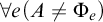 . Let
$R_e$
 denote the formula
$A\neq \Phi _e$
 and call it a requirement; we say that
$R_e$
 is satisfied (in M) if
$M\models R_e$
 . If all requirements are satisfied, then
$M\models \forall e\, R_e$
 , so A is noncomputable. We will also use an order-preserving map
$\lambda : M\to M$
 , whose domain indexes the requirements, with
$\lambda (e)$
 the priority of the e-th requirement. In a standard model this is usually a bijection, but in a nonstandard model it may be neither injective nor surjective; this is the block method, introduced in Section 3.3. The construction proceeds stage by stage. At each stage s, we attempt to satisfy the requirements of index
$<s$
 , possibly enumerating some elements into the c.e. set A. By the end of the stage,
$A_s$
 is completely determined, and the sequence
$\{A_s\}_{s\in M}$
 is the enumeration of the c.e. set A. Since different requirements may impose conflicting demands on A, we use the priority given by
$\lambda $
 to resolve these conflicts. For clarity, a requirement can be visited, act, be injured, or be initialized. When a requirement is visited, we run its predesigned procedure, called its strategy: if a prescribed event is observed, the requirement acts; otherwise, the next requirement is visited. Whenever a requirement acts, the requirements of lower priority are deemed injured, since their strategies may no longer lead to satisfaction, and we initialize them. Initialization has two effects: each initialized requirement restarts its strategy anew at the next stage it is visited, and it respects everything done so far, such as the restraint imposed by a requirement of higher priority. Consequently, requirements of lower priority cannot injure those of higher priority. It then remains to show that, for each requirement, there is a stage after which it is never initialized again (equivalently, requirements of higher priority no longer act), so that its strategy leads to satisfaction within finitely many stages.
Let us summarize all conventions that will be assumed during our construction:
-
(i) We adopt the standard convention that at stage s, all numbers that appear in the construction are less than s.
-
(ii) When a requirement acts, the requirements of lower priority are regarded as injured (whether or not they actually are) and hence initialized: all their work is canceled, and each restarts anew at the next stage it is visited.
-
(iii) If A is a c.e. set to be constructed, its elements are enumerated at certain stages, and we let $A_s$
collect the elements enumerated by the end of stage s. Thus
$A_s$
is defined for every
$s\in M$
, with
$A_s=A_{s-1}$
at any stage that enumerates nothing into A. -
(iv) If $\Delta $
is a Turing functional to be constructed, then at stage s we define
$\Delta _s^\sigma (x)=k$
to mean that we enumerate the axiom
$\langle x,k,\sigma ^1,\sigma ^0\rangle $
into
$\Delta $
, and we define
$\Delta _s(x)=k$
to mean that we enumerate the axiom
$\langle x,k,\varnothing ,\varnothing \rangle $
into
$\Delta $
. Here the subscript s is added for clarity. By Item (1b) of Definition 2.5, all extensions of these axioms belong to
$\Delta $
automatically, so we need not enumerate them explicitly. As with
$A_s$
, we let
$\Delta _s$
collect the axioms enumerated into
$\Delta $
by the end of stage s; it is thereby defined for every
$s\in M$
, with
$\Delta _s=\Delta _{s-1}$
at any stage that enumerates no new axiom into
$\Delta $
.


The rest of the article is organized as follows. Section 3 recalls the proof of the Sacks Splitting Theorem; Section 4 builds on it to prove the Robinson Splitting Theorem; and Section 5 contains some discussion and open questions.
3 Proof of the Sacks Splitting Theorem (Theorem 1.1)
We will prove a slightly stronger statement, with a cone-avoidance property added. That is, given a c.e. degree
$\boldsymbol {b}$
 and a noncomputable c.e. degree
$\boldsymbol {d}$
 , there exist incomparable c.e. degrees
$\boldsymbol {a_0}$
 and
$\boldsymbol {a_1}$
 such that
$\boldsymbol {b}=\boldsymbol {a_0}\vee \boldsymbol {a_1}$
 and
$\boldsymbol {d}\nleq \boldsymbol {a_i}$
 for
$i<2$
 .
Let M be a model of
$\mathsf {P}^-+\mathsf {I}\Sigma _1$
 . Given c.e. sets
$B,D\subseteq M$
 with D noncomputable, let the enumeration of B be given by Lemma 2.14. We exhibit c.e. sets
$A_0,A_1\subseteq M$
 such that
$B=A_0\sqcup A_1$
 (so
$B\equiv _{sT} A_0\oplus A_1$
 ) and
$D\nleq _{pT} A_i$
 for
$i<2$
 . Since
$D\nleq _{pT} A_i$
 implies
$D\nleq _{sT} A_i$
 , this yields the desired conclusion on Turing degrees. Taking
$D=B$
 gives the original theorem.
We have a global requirement that
$B=A_0\sqcup A_1$
 . The other requirements to satisfy are the following:

where
$\Delta _e$
 and
$\Gamma _e$
 are Turing functionals built locally by the corresponding requirement and canceled when that requirement is initialized. Given that D is noncomputable, once the requirements are satisfied for all
$e\in M$
 , we are done. We remark that the injury set
$I_e=\{s\mid P_e\text { is injured at }s\}$
 is
$\Sigma _1$
 . However, the statement that
$I_e$
 is finite is
$\Sigma _2$
 . The following induction only works over
$\mathsf {I}\Sigma _2$
 :

To resolve this, as in Mytilinaios’ paper [Reference Shore17], there are two ideas: the first is the blocking method, and the second is to use dynamic priority assignments. We first review the basic strategy of the Sacks Splitting Theorem.
3.1 A single requirement
Without loss of generality, we describe the strategy for a single
$P_e$
 -requirement, and we assume for now that it is never initialized (equivalently, never injured); the
$Q_e$
 -requirements are treated symmetrically.
The rough idea for satisfying the
$P_e$
 -requirement is to copy agreements between D and
$\Phi _e^{A_0}$
 into
$\Delta _e$
 and protect the underlying computations, so that any later change in D exposes a disagreement.
If
$P_e$
 is visited at stage s, we call s a
$P_e$
 -stage. Let

be the length of agreement between
$\Phi _e^{A_0}$
 and D at stage s. A
$P_e$
 -stage s is
$P_e$
 -expansionary if
$\ell _s(e)>\ell _t(e)$
 for every
$P_e$
 -stage
$t<s$
 .
$\boldsymbol {P}_{\boldsymbol {e}}$
 -strategy
: Suppose
$P_e$
 is visited at stage s, and let
$s^-<s$
 be the previous
$P_e$
 -stage.
-
(1) If $P_e$
has already been declared to diagonalize, do nothing. -
(2) Otherwise, if $D_s(x)\neq \Delta _{e,s^-}(x)$
for some
$x\in \operatorname {\mathrm {dom}} \Delta _{e,s^-}$
, then
$P_e$
acts and we declare that
$P_e$
diagonalizes at x. -
(3) Otherwise, if s is $P_e$
-expansionary, then
$P_e$
acts: for every
$x\le \ell _s(e)$
with
$x\notin \operatorname {\mathrm {dom}} \Delta _{e,s^-}$
, we define
$\Delta _{e,s}(x)=D_s(x)$
and record the fixing triple
$(\sigma ,x,k)$
, where
$\sigma =A_{0,s}\!\upharpoonright \! s$
and
$k=D_s(x)$
. -
(4) Otherwise (s is a $P_e$
-stage that is not expansionary), do nothing.









Note that once
$\Delta _{e,s}(x)$
 is defined, it is never redefined, so its value is permanent. Whenever
$P_e$
 acts at stage s, we set the restraint
$\rho _s(e)=s$
 and initialize all requirements of lower priority; thereafter no requirement of lower priority enumerates into
$A_0$
 any element less than
$\rho _s(e)=s$
 . Consequently, for every fixing triple
$(\sigma ,x,k)$
 recorded at stage s, the final set
$A_0$
 satisfies
$A_0\in [\sigma ]$
 , and hence
$\Phi _e^{A_0}(x)=k=\Delta _e(x)$
 . In particular, for every
$x\in \operatorname {\mathrm {dom}}\Delta _e$
 ,

We verify that
$P_e$
 is satisfied in two cases.
Case 1: Item (2) occurs, say at stage s witnessed by some x. Since D is c.e., its value never decreases, so
$D(x)=D_s(x)\neq \Delta _{e,s^-}(x)=\Delta _e(x)$
 . By the equivalence above,
$D(x)\neq \Phi _e^{A_0}(x)$
 , so
$P_e$
 is satisfied. From stage s onward, Item (1) applies at every
$P_e$
 -stage, so
$P_e$
 never acts again.
Case 2: Item (2) never occurs. Then
$\Delta _e(x)=D(x)$
 for every
$x\in \operatorname {\mathrm {dom}}\Delta _e$
 . If
$\operatorname {\mathrm {dom}}\Delta _e=M$
 , then
$\Delta _e=D$
 would be computable, contradicting the noncomputability of D; hence
$\operatorname {\mathrm {dom}}\Delta _e\neq M$
 . By
$\mathsf {L}\Pi _1$
 , let a be the least element of
$M\setminus \operatorname {\mathrm {dom}}\Delta _e$
 . For every
$x<a$
 we have
$x\in \operatorname {\mathrm {dom}}\Delta _e$
 , so
$D(x)=\Delta _e(x)=\Phi _e^{A_0}(x)$
 . We claim that
$D(a)\neq \Phi _e^{A_0}(a)$
 . Let s be the stage at which
$\Delta _e(a-1)$
 is defined if
$a>0$
 , and
$s=0$
 if
$a=0$
 (so that
$\operatorname {\mathrm {dom}}\Delta _e=\varnothing $
 ). No
$P_e$
 -stage
$t>s$
 is expansionary, since otherwise
$\ell _t(e)\ge a$
 would force
$a\in \operatorname {\mathrm {dom}}\Delta _e$
 . Hence
$D(a)\neq \Phi _e^{A_0}(a)$
 , so
$P_e$
 is satisfied. Moreover, only Item (4) applies after stage s, so
$P_e$
 never acts again.
We summarize this discussion as follows.
Lemma 3.1. Suppose there is a stage
$s_0$
 after which
$P_e$
 (resp.
$Q_e$
 ) is never initialized. Then
$P_e$
 (resp.
$Q_e$
 ) is satisfied, and there is a stage
$s_1>s_0$
 after which it never acts. Moreover, the restraint it imposes on
$A_0$
 (resp.
$A_1$
 ) is bounded by
$s_1$
 .
3.2 A block of requirements
To carry out the proof in an
$\mathsf {I}\Sigma _1$
 model, Mytilinaios [Reference Mytilinaios12] adapted the blocking method from
$\alpha $
 -recursion theory. We review this technique here. The set
$\Lambda =\{P_{e_0},P_{e_0+1},\dots , P_{e_1}\}$
 is referred to as a block of P-requirements (the Q-requirements are treated the same way). Requirements in the same block have the same priority order; if one requirement in the block is initialized, all are initialized. In this case, we say that the block
$\Lambda $
 is initialized. If one of the requirements acts, we say that the block
$\Lambda $
 acts. For notational convenience, we also conflate the set
$\Lambda $
 with the set of indices
$\{e_0,e_0+1,\dots , e_1\}$
 , so
$P_e\in \Lambda $
 and
$e\in \Lambda $
 are both valid.
We suppose
$s_0$
 is a stage after which no requirement in the block
$\Lambda $
 is initialized. Since P-requirements impose restraint only on
$A_0$
 , there are no conflicts between requirements in
$\Lambda $
 . We let each requirement in
$\Lambda $
 follow the same strategy as in the single-requirement case. As pointed out in Lemma 3.1, for each requirement in
$\Lambda $
 , there exists some stage after which it stops acting; however, it is not obvious that there exists a stage after which no requirement in
$\Lambda $
 acts. We prove this.
Note that once
$P_e$
 diagonalizes, it will never have another expansionary stage. Let
$f:\Lambda \to M$
 be defined by
$f(e)=s$
 if
$P_e$
 diagonalizes at stage s. Since f is partial computable with bounded domain,
$\operatorname {\mathrm {ran}} f$
 is bounded by some
$s_1$
 by Lemma 2.9. Moreover,
$\operatorname {\mathrm {dom}} f$
 is a bounded c.e. subset of M and is therefore M-finite.
Let
$\Lambda _1=\Lambda \setminus \operatorname {\mathrm {dom}} f$
 , an M-finite set. For each
$e\in \Lambda _1$
 ,
$P_e$
 never diagonalizes. That is, if
$\Delta _{e,s}(x)=D_s(x)$
 is defined at stage s, then it is permanently correct; otherwise,
$e\in \operatorname {\mathrm {dom}} f$
 , contradicting the choice of
$\Lambda _1$
 .
Now, we claim that
$\bigcup _{e\in \Lambda _1} \operatorname {\mathrm {dom}} \Delta _e \neq M$
 . Suppose otherwise that
$\bigcup _{e\in \Lambda _1} \operatorname {\mathrm {dom}} \Delta _e = M$
 ; then for each
$x\in M$
 and each
$i\in \{0,1\}$
 ,

which shows that both D and
$\bar {D}$
 are c.e., so D is computable, contradicting the noncomputability of D.
Since for each
$e\in \Lambda _1$
 ,
$\operatorname {\mathrm {dom}} \Delta _e$
 is an initial segment of M (by construction),
$\bigcup _{e\in \Lambda _1}\operatorname {\mathrm {dom}} \Delta _e$
 is bounded by some b.
Let
$g:\Lambda _1\times b\to M$
 be defined by
$g(e,x)=s$
 if
$\Delta _{e,s}(x)$
 is defined at stage s. Since g is partial computable with bounded domain,
$\operatorname {\mathrm {ran}} g$
 is bounded by some
$s_2>s_1$
 by Lemma 2.9. That is, after stage
$s_2$
 , no requirement in
$\Lambda _1$
 has another expansionary stage, and hence none acts again.
To summarize, we have the following lemma.
Lemma 3.2. Suppose there exists some
$s_0$
 after which the requirements in
$\Lambda $
 (resp.
$\Upsilon $
 ) are not initialized. Then all requirements in
$\Lambda $
 (resp.
$\Upsilon $
 ) are satisfied, and there exists some stage
$s_2>s_0$
 after which
$\Lambda $
 (resp.
$\Upsilon $
 ) no longer acts. Moreover, the overall restraint imposed by
$\Lambda $
 (resp.
$\Upsilon $
 ) on
$A_0$
 (resp.
$A_1$
 ) is bounded by
$s_2$
 .
In other words, after stage
$s_2$
 , requirements of lower priority will not be injured by
$\Lambda $
 and can safely follow their strategies.
We remark that the Robinson case (Lemma 4.5) is substantially more subtle than Lemma 3.2, and its proof requires the full strength of both the hyperregularity of C and the fact that
$C'$
 is
$\omega $
 -c.e. These properties are essential for bounding the overall restraint.
3.3 Dynamic priority assignments
A priority assignment consists of two computable functions
$\lambda :\{P_e\mid e\in M\}\to M$
 and
$\mu :\{Q_e\mid e\in M\}\to M$
 such that, for all
$e\in M$
 ,
$\lambda (P_{e+1})\ge \lambda (P_e)$
 and
$\mu (Q_{e+1})\ge \mu (Q_e)$
 , and the ranges of
$\lambda $
 and
$\mu $
 are initial segments of M. We let

be the blocks of P-requirements and Q-requirements of order i, respectively; requirements in the same block have the same priority. Requirements of different types are ordered by
$\Lambda (0)<\Upsilon (0)<\Lambda (1)<\Upsilon (1)<\cdots $
 .
A dynamic priority assignment consists of two uniformly computable sequences
$\{\lambda _s\}_{s\in M}$
 and
$\{\mu _s\}_{s\in M}$
 such that each pair
$\lambda _s,\mu _s$
 is a priority assignment and, for each
$e\in M$
 ,
$\lambda _{s+1}(P_e)\le \lambda _s(P_e)$
 and
$\mu _{s+1}(Q_e)\le \mu _s(Q_e)$
 . With respect to
$\lambda _s$
 and
$\mu _s$
 , we set
$\Lambda _s(i)=\lambda _s^{-1}(i)$
 and
$\Upsilon _s(i)=\mu _s^{-1}(i)$
 ; these are again ordered by priority as
$\Lambda _s(0)<\Upsilon _s(0)<\Lambda _s(1)<\Upsilon _s(1)<\cdots $
 .
Lemma 3.3. For each
$e\in M$
 ,
$\lim _s \lambda _s(P_e)$
 and
$\lim _s \mu _s(Q_e)$
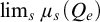 exist.
Proof. The set
$\{i\mid \exists s (\lambda _s(P_e)=i)\}$
 is a
$\Sigma _1$
 set and so it has a least element
$i_0$
 by
$\mathsf {L}\Sigma _1$
 . Since
$\lambda _{s+1}(P_e)\le \lambda _s(P_e)$
 , we have
$\lim _s \lambda _s(P_e)=i_0$
 . Similarly,
$\lim _s \mu _s(Q_e)$
 exists.
So each
$P_e$
 -requirement (resp.
$Q_e$
 -requirement) reaches its “final” priority order at some stage.
Next, we describe how the dynamic priority assignment is defined. Initially, we set
$\lambda _0(P_e)=\mu _0(Q_e)=e$
 for all
$e\in M$
 .
At stage
$s>0$
 , we run the construction with respect to
$\lambda _{s-1}$
 and
$\mu _{s-1}$
 . Then we may decide to reassign some block. If no block is reassigned, we leave the priority unchanged at the end of stage s:
$\lambda _{s}(P_e)=\lambda _{s-1}(P_e)$
 and
$\mu _s(Q_e)=\mu _{s-1}(Q_e)$
 for all
$e\in M$
 .
If
$\Upsilon _{s-1}(i)$
 is reassigned at stage s, we let
$Q_n$
 be the last requirement in
$\Upsilon _{s-1}(i)$
 ; that is,
$Q_n\in \Upsilon _{s-1}(i)$
 and
$Q_{n+1}\notin \Upsilon _{s-1}(i)$
 . Then we define
$\mu _s$
 as follows:
-
• $\mu _s(Q_j)=\mu _{s-1}(Q_j)$
for all
$j\le n$
; -
• $\mu _s(Q_j)=i$
for all
$n<j\le s$
; -
• $\mu _s(Q_j)=\mu _s(Q_s)+(j-s)$
for all
$j>s$
.


That is, the block
$\Upsilon _{s-1}(i)$
 expands to
$\Upsilon _s(i)$
 by absorbing sufficiently many Q-requirements. Symmetrically, if
$\Lambda _{s-1}(i)$
 is reassigned at stage s, we let
$P_m$
 be the last requirement in
$\Lambda _{s-1}(i)$
 ; that is,
$P_m\in \Lambda _{s-1}(i)$
 and
$P_{m+1}\notin \Lambda _{s-1}(i)$
 . Then we define
$\lambda _s$
 as follows:
-
• $\lambda _s(P_j)=\lambda _{s-1}(P_j)$
for all
$j\le m$
; -
• $\lambda _s(P_j)=i$
for all
$m<j\le s$
; -
• $\lambda _s(P_j)=\lambda _s(P_s)+(j-s)$
for all
$j>s$
.


That is, the block
$\Lambda _{s-1}(i)$
 expands to
$\Lambda _s(i)$
 by absorbing sufficiently many P-requirements.
Lemma 3.4. For each
$e,s\in M$
 with
$s\ge 1$
 ,
$\lambda _{s}(P_e)\le \lambda _{s-1}(P_e)$
 and
$\mu _{s}(Q_e)\le \mu _{s-1}(Q_e)$
 .
Proof. We take
$\mu _s(Q_e)$
 as an example. The proof for
$\lambda _s(P_e)$
 is analogous. We prove the claim by induction on s. The base case
$s=1$
 is obvious. Note that for each
$s\le j$
 ,
$\mu _s(Q_j)-\mu _s(Q_s)=j-s$
 . Let
$Q_n$
 be the last requirement in
$\Upsilon _{s-1}(i)$
 . If
$e\le n$
 , then
$\mu _s(Q_e)=\mu _{s-1}(Q_e)$
 ; if
$n<e\le s$
 , then
$\mu _s(Q_e)=i=\mu _{s-1}(Q_n)<\mu _{s-1}(Q_e)$
 ; if
$s<e$
 , then
$\mu _s(Q_e)=\mu _s(Q_s)+(e-s)=\mu _s(Q_s)+\mu _{s-1}(Q_{e-1})-\mu _{s-1}(Q_{s-1})$
 . With
$\mu _s(Q_s)\le \mu _{s-1}(Q_s)=\mu _{s-1}(Q_{s-1})+1$
 and
$\mu _{s-1}(Q_e)=\mu _{s-1}(Q_{e-1})+1$
 , we obtain
$\mu _s(Q_e)\le \mu _{s-1}(Q_e)$
 .
Therefore, the dynamic priority assignment indeed satisfies the required properties, and Lemma 3.3 applies to our construction. We let

be the final blocks of P-requirements and Q-requirements of order i, respectively. We have the following lemma.
Lemma 3.5. If
$\Lambda _s(i)$
 (resp.
$\Upsilon _s(i)$
 ) is not reassigned at any stage
$s\ge s_0$
 , then
$\Lambda (i)=\Lambda _{s_0}(i)$
 (resp.
$\Upsilon (i)=\Upsilon _{s_0}(i)$
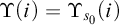 ).
Next, we present the construction and verification.
3.4 The construction and verification
Let us now introduce the restraint function. The restraint set by
$\Lambda _s(i)$
 is denoted by
$\rho _s(i)$
 , and the restraint set by
$\Upsilon _s(i)$
 is denoted by
$\tau _s(i)$
 . If no restraint has been set, we let
$\rho _s(i)=\tau _s(i)=-1$
 ; if we do not explicitly define
$\rho _s(i)$
 or
$\tau _s(i)$
 , it defaults to
$\rho _s(i)=\rho _{s-1}(i)$
 or
$\tau _s(i)=\tau _{s-1}(i)$
 , respectively. If
$\Lambda _{s-1}(i)$
 or
$\Upsilon _{s-1}(i)$
 is initialized at stage s, then we define
$\rho _s(i)=-1$
 or
$\tau _{s}(i)=-1$
 . For a number
$x\in M$
 , we say x threatens
$\Lambda _s(i)$
 or
$\Upsilon _s(i)$
 if
$x\le \rho _s(i)$
 or
$x\le \tau _s(i)$
 , respectively.
By Lemma 2.14, we may fix an enumeration
$\{B_s\}_{s\in M}$
 of B such that, for each s, the set
$B_s\setminus B_{s-1}$
 are empty or a singleton, and is empty whenever s is even.
The construction: At stage s, if
$B_s\setminus B_{s-1}\neq \varnothing $
 , we call s an enumeration stage and carry out Part I; otherwise, if
$B_s = B_{s-1}$
 , we call s a strategy stage and carry out Part II. Note that every even stage is a strategy stage, and that at a strategy stage no element is enumerated into
$A_0$
 or
$A_1$
 , so
$A_{0,s}=A_{0,s-1}$
 and
$A_{1,s}=A_{1,s-1}$
 .
Part I. Enumeration of
$A_0$
 and
$A_1$
 : Let
$x\in B_s\setminus B_{s-1}$
 . Let
$\Lambda _{s-1}(i)$
 (resp.
$\Upsilon _{s-1}(i)$
 ) be the highest-priority block that x threatens, if such a block exists.
-
(i.1) If it is $\Lambda _{s-1}(i)$
, enumerate x into
$A_1$
, initialize all blocks of priority lower than
$\Lambda _{s-1}(i)$
, and reassign
$\Upsilon _{s-1}(i)$
and
$\Lambda _{s-1}(i+1)$
. -
(i.2) Otherwise, if it is $\Upsilon _{s-1}(i)$
, enumerate x into
$A_0$
, initialize all blocks of priority lower than
$\Upsilon _{s-1}(i)$
, and reassign
$\Lambda _{s-1}(i+1)$
and
$\Upsilon _{s-1}(i+1)$
.


If no block is threatened, enumerate x into
$A_0$
 and leave the priority unchanged.
This ends the current stage.
Part II. Block strategy: We begin by visiting
$\Lambda _{s-1}(0)$
 . Suppose, without loss of generality, that the block
$\Lambda _{s-1}(i)$
 is visited (the case of
$\Upsilon _{s-1}(i)$
 is symmetric).
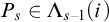
-
(ii.1) If $P_s\in \Lambda _{s-1}(i)$
, leave the priority unchanged and end the current stage. -
(ii.2) Otherwise, for each $P_e\in \Lambda _{s-1}(i)$
, perform the
$P_e$
-strategy presented in Section 3.1, which we repeat here for convenience:-
(a) If $P_e$
has already been declared to diagonalize, do nothing. -
(b) Otherwise, if $D_s(x)\neq \Delta _{e,s^-}(x)$
for some
$x\in \operatorname {\mathrm {dom}} \Delta _{e,s^-}$
, then
$P_e$
acts and we declare that
$P_e$
diagonalizes at x. -
(c) Otherwise, if s is $P_e$
-expansionary, then
$P_e$
acts: for every
$x\le \ell _s(e)$
with
$x\notin \operatorname {\mathrm {dom}} \Delta _{e,s^-}$
, we define
$\Delta _{e,s}(x)=D_s(x)$
and record the fixing triple
$(\sigma ,x,k)$
, where
$\sigma =A_{0,s}\!\upharpoonright \! s$
and
$k=D_s(x)$
. -
(d) Otherwise (s is a $P_e$
-stage that is not expansionary), do nothing.
-
-
(ii.3) If one of the requirements acts, we say that the block acts: set the restraint $\rho _s(i)=s$
, initialize all blocks of priority lower than
$\Lambda _{s-1}(i)$
, reassign
$\Upsilon _{s-1}(i)$
and
$\Lambda _{s-1}(i+1)$
, and end the current stage. -
(ii.4) Otherwise, if no requirement acts, leave the restraint unchanged ( $\rho _s(i)=\rho _{s-1}(i)$
) and visit
$\Upsilon _{s-1}(i)$
, the block of next-highest priority.










This completes the construction.
We now proceed to the verification, using Lemmas 3.1, 3.2, and 3.5, which have already been proved.
Lemma 3.6. Suppose
$\Lambda _{s-1}(i)$
 (resp.
$\Upsilon _{s-1}(i)$
 ) is initialized at stage s. Then for some
$j\le i$
 ,
$\Lambda _{s-1}(j)$
 (resp.
$\Upsilon _{s-1}(j)$
 ) is reassigned at stage s.
Proof. This follows immediately from the construction.
Lemma 3.7. Suppose
$\Lambda _{s-1}(i)$
 (resp.
$\Upsilon _{s-1}(i)$
 ) is not initialized at any stage
$s>s_0$
 . Then there exists some stage
$s_1> s_0$
 after which
$\Upsilon _{s-1}(i)$
 (resp.
$\Lambda _{s-1}(i+1)$
 ) is not initialized at any stage
$s> s_1$
 .
Proof. We take
$\Lambda _s(i)$
 as an example; the case of
$\Upsilon _s(i)$
 is similar. Since
$\Lambda _s(i)$
 is not initialized at any stage
$s>s_0$
 , it is not reassigned at any such stage. By Lemma 3.5,
$\Lambda (i)=\Lambda _{s_0}(i)$
 . Applying Lemma 3.2 to
$\Lambda (i)$
 , we obtain a stage
$s^*> s_0$
 such that
$\Lambda (i)$
 does not act after
$s^*$
 , and the restraint imposed on
$A_0$
 is bounded by
$s^*$
 . There exists a stage
$s_1> s^*$
 such that no
$x \leq s^*$
 is enumerated into B after
$s_1$
 . Hence, by Part I of the construction,
$\Lambda (i)$
 is not threatened after
$s_1$
 . Thus,
$\Upsilon _{s-1}(i)$
 is not initialized at any stage
$s>s_1$
 .
Lemma 3.8. For each
$e \in M$
 ,
$P_e$
 and
$Q_e$
 are satisfied.
Proof. The case for
$Q_e$
 is analogous; we take
$P_e$
 as an example. By Lemma 3.5, the limit
$i = \lim _s \lambda _s(P_e)$
 exists; it is the final priority order of
$P_e$
 . Let
$s_0$
 be the first stage at which
$\lambda _s(P_e) = i$
 . For each
$s> s_0$
 ,
$\Lambda _{s-1}(i-1)$
 is not initialized at stage s, since otherwise, Lemma 3.6 shows that
$\lambda _s(P_e) \leq i-1$
 . By Lemma 3.7, there exists some stage
$s_1> s_0$
 such that
$\Upsilon _s(i-1)$
 is not initialized at any stage
$s>s_1$
 . By the same lemma, there exists some stage
$s_2> s_1$
 such that
$\Lambda _{s-1}(i)$
 is not initialized at any stage
$s>s_2$
 . By Lemma 3.2,
$P_e$
 is satisfied.
This completes the proof of Theorem 1.1. Based on this construction, we prove the main theorem in the next section.
We emphasize that the use of
$\mathsf {I}\Sigma _1$
 is crucial in the proof of Lemma 3.2 (see Section 3.2), especially in establishing that the restraint imposed on
$A_0$
 is bounded. In this argument, it is essential that D is c.e.: this ensures that the auxiliary function f is
$\Sigma _1$
 , so that the boundedness argument can be carried out in
$\mathsf {I}\Sigma _1$
 .
If D were not c.e., then f would no longer be
$\Sigma _1$
 , and the proof given here would break down over
$\mathsf {I}\Sigma _1$
 . In the standard model
$\mathbb {N}$
 , by contrast, D could be any
$\Delta ^0_2$
 set, and only minor modifications to the construction would be needed.
There is a simple workaround when D is n-c.e. in models of
$\mathsf {I}\Sigma _1$
 , for the case when
$n\in \mathbb {N}$
 is a standard natural number. Since every noncomputable n-c.e. set computes a noncomputable c.e. set, let
$E\le _T D$
 be such a c.e. set; then it suffices to avoid the upper cone of E in the construction. The corresponding question for arbitrary D remains open.
4 Proof of the Robinson Splitting Theorem (Theorem 1.3)
For the reader’s convenience, we restate the theorem. Let
$M\models \mathsf {P}^-+\mathsf {I}\Sigma _1$
 . Given c.e. degrees
$\boldsymbol {b},\boldsymbol {c},\boldsymbol {d}$
 with
$\boldsymbol {c}$
 super-low and
$\boldsymbol {d}\nleq \boldsymbol {c}$
 , there exist incomparable c.e. degrees
$\boldsymbol {a_0},\boldsymbol {a_1}$
 such that
$\boldsymbol {b}= \boldsymbol {a_0}\vee \boldsymbol {a_1}$
 and
$\boldsymbol {d}\nleq \boldsymbol {a_i}\vee \boldsymbol {c}$
 for
$i<2$
 .
We fix a model M of
$\mathsf {P}^- +\mathsf {I}\Sigma _1$
 . Let
$B, C, D \subseteq M$
 be c.e. sets with C super-low (and therefore hyperregular by Corollary 2.19, and
$C\le _{sT} K$
 by Lemma 2.17) and
$D \nleq _{sT} C$
 (equivalent to
$D\nleq _{pT} C$
 by Corollary 2.7). Let the enumeration of B be given by Lemma 2.14. We exhibit c.e. sets
$A_0$
 and
$A_1$
 such that
$B = A_0 \sqcup A_1$
 (so
$B\equiv _{sT} A_0\oplus A_1$
 ), satisfying the following requirements for each
$e \in M$
 :

Here,
$\Delta _e$
 and
$\Gamma _e$
 are Turing functionals built locally by the corresponding requirement and canceled when that requirement is initialized. If the requirements are satisfied for all
$e\in M$
 , then
$D\nleq _{pT} A_i\oplus C$
 and therefore
$D\nleq _{sT} A_i\oplus C$
 for
$i<2$
 , which yields the desired conclusion.
The overall framework is the same as in the proof of the Sacks Splitting Theorem. Recall from Section 3.4 that a stage s is an enumeration stage if
$B_s\setminus B_{s-1}\neq \varnothing $
 , and a strategy stage if
$B_s = B_{s-1}$
 . At an enumeration stage we do the same thing, and the dynamic priority assignment is defined in the same way. We shall focus on the strategy for satisfying a single
$P_e$
 -requirement (the
$Q_e$
 -requirements are treated symmetrically) and then a block of requirements.
Robinson’s trick is to consider

X is
$\Sigma _1^C$
 and therefore,

Since
$C'$
 is
$\omega $
 -c.e., so is X. Let p and q be computable functions (by Definition 2.13) such that

$p(j,0)=0$
 and

4.1 Certified computation
The main difficulty in satisfying a P-requirement (resp. Q-requirement) is that we are unable to preserve a computation
$\Phi _{e,s}^{A_{0,s}\oplus C_s}(x)=k$
 with axiom
$(\theta , \sigma , x, k)$
 at stage s. By imposing a restraint on
$A_0\!\upharpoonright \! s$
 , we can ensure that
$A_0\in [\theta ]$
 ; however, C is not restrained, so we must guess whether
$C\in [\sigma ]$
 . A computation is tested for certification: if we guess that
$C\in [\sigma ]$
 (made precise below), we call it certified; if it is evident that
$C\notin [\sigma ]$
 , we treat the computation as divergent and call it not certified. Our guess may be wrong; super-lowness controls the number of wrong guesses, and this is what makes the strategy terminate in M-finitely many stages.
To implement the
$P_e$
 -strategy (the
$Q_e$
 -strategy is similar), we work one input at a time. For each
$x\in M$
 , we consider the subrequirement

All of the certification machinery below is developed for a fixed subrequirement
$P_e(x)$
 ; throughout, e and x are fixed.
Suppose at stage s, we observe
$\Phi _{e,s}^{A_{0,s}\oplus C_s}(x)\downarrow = k$
 . Let
$l=\varphi _{e,s}^{A_{0,s}\oplus C_s}(x)$
 ,
$\theta =A_{0,s}\!\upharpoonright \! l$
 , and
$\sigma = C_s\!\upharpoonright \! l$
 . We refer to
$\Phi _{e,s}^{A_{0,s}\oplus C_s}(x)\downarrow $
 as a computation and
$(\theta , \sigma , x, k)$
 as its axiom.
To certify a computation, we use a c.e. set
$W_j$
 , called the guessing set. Here, the index j is given by the recursion theorem (see Theorem 2.20 and Remark 4.2).
$W_{j,s}$
 denotes the elements enumerated into
$W_j$
 by the end of stage s.
Suppose that at stage s, we have a computation
$\Phi _{e,s}^{A_{0,s}\oplus C_s}(x)\downarrow =k$
 with axiom
$(\theta ,\sigma ,x,k)$
 . If
$C_s\in [W_{j,s-1}]$
 , that is, the computation has already been tested for certification, we do nothing. Otherwise, if
$C_s\notin [W_{j,s-1}]$
 , the certification procedure is as follows:
-
(C.1) Enumerate $\sigma $
into
$W_j$
(so
$C_s\in [W_{j,s}]$
). -
(C.2) Let $t \ge s$
be the least stage such that either
$C_t \notin [\sigma ]$
or
$p(j, t) = 1$
.-
(C.2a) If $C_t \notin [\sigma ]$
, this computation is not certified. -
(C.2b) If $p(j, t) = 1$
, this computation is certified. In this case,
$P_e(x)$
acts: impose a restraint on
$A_0\!\upharpoonright \! s$
.
-


Item (C.2) assumes
$C_s\in [W_{j,s}]$
 , so the stage t exists since

In Item (C.2a),
$C_t\notin [\sigma ]$
 evidently implies
$C\notin [\sigma ]$
 , so we treat the computation as divergent and do not impose restraint on
$A_0$
 , allowing elements to be enumerated into
$A_0$
 . In Item (C.2b),
$p(j,t)=1$
 indicates that
$C\in [\sigma ]$
 is more likely; we impose a restraint on
$A_0\!\upharpoonright \! s$
 to preserve the computation with axiom
$(\theta ,\sigma ,x,k)$
 . This is still a guess, and elements below s can still be enumerated into C after stage t.
For clarity, suppose
$(\theta ,\sigma ,x,k)$
 is the axiom of a computation certified at stage s. We say that this certified computation becomes injured at stage
$u>s$
 if
$C_u\in [\sigma ]$
 but
$A_{0,u}\notin [\theta ]$
 ; equivalently, our restraint imposed on
$A_0\!\upharpoonright \! s$
 fails at stage u. If this happens, we cannot certify any further computations using the same guessing set
$W_j$
 , since it may turn out that
$C\in [\sigma ]$
 and all subsequent computations would be certified automatically. If any certified computation is injured, we say that the subrequirement
$P_e(x)$
 is injured. We refresh the index j of the guessing set
$W_j$
 if and only if
$P_e(x)$
 is injured. If the
$P_e$
 -requirement is initialized, we also consider
$P_e(x)$
 to be injured.
Lemma 4.1. Suppose
$P_e(x)$
 is not injured after
$s_0$
 . Then there exists some stage
$s_1>s_0$
 after which
$P_e(x)$
 does not act. Moreover, the restraint imposed on
$A_0$
 is bounded by
$s_1$
 .
Proof. If
$\lim _s p(j,s)=1$
 , then
$C\in [W_j]$
 . Let
$\sigma \in W_j$
 be the finite string with
$C\in [\sigma ]$
 enumerated into
$W_j$
 at stage
$s_1>s_0$
 ; then
$C\in [W_{j,s_1}]$
 , so
$P_e(x)$
 does not perform the certification procedure after stage
$s_1$
 and does not act thereafter.
If
$\lim _s p(j,s)=0$
 , let
$s_1$
 be the stage such that for all
$s>s_1$
 ,
$p(j,s)=0$
 . After
$s_1$
 , no computation can be certified, since Item (C.2b) never applies. Therefore,
$P_e(x)$
 does not act after stage
$s_1$
 .
Remark 4.2. The index of the guessing set depends on e, x, the number of times k that
$P_e(x)$
 is injured, and the number j that appears in Item (C.2). Indeed, there exists a computable function f such that the guessing set is
$W_{f(j,e,x,k)}$
 ; if
$P_e(x)$
 is injured at stage s, then the guessing set at stage
$s+1$
 is
$W_{f(j,e,x,k+1)}$
 . For a general number j, the certification procedure would not work, since
$W_{f(j,e,x,k)}\neq W_j$
 . However, by the recursion theorem, there exists a computable function g such that for all
$e,x,k$
 ,

So the certification procedure works by replacing the number j in Item (C.2) with
$g(e,x,k)$
 .
In the rest of the article, we assume that we know the index beforehand by the recursion theorem.
4.2 Single requirement
We take the
$P_e$
 -requirement as an example. In the previous section, we showed how to certify a computation for a subrequirement
$P_e(x)$
 and why it is useful (Lemma 4.1). In this section, we first present the
$P_e(x)$
 -strategy and then assemble the subrequirements into the full
$P_e$
 -strategy.
$\boldsymbol {P}_{\boldsymbol {e}}\boldsymbol {(x)}$
 -strategy
: At stage s, let j be the index of the guessing set, given by the recursion theorem (see Remark 4.2). We proceed as follows:
-
(Px.1) If $\Phi _{e,s}^{A_{0,s}\oplus C_s}(x)\uparrow $
or
$\Phi _{e,s}^{A_{0,s}\oplus C_s}(x)\downarrow \neq D_s(x)$
, we do nothing. -
(Px.2) Otherwise, if $\Delta _{e,s-1}^{C_s}(x)\downarrow $
, we do nothing. -
(Px.3) Otherwise, if $\Delta _{e,s-1}^{C_s}(x)\uparrow $
and
$\Phi _{e,s}^{A_{0,s}\oplus C_s}(x)\downarrow = D_s(x)=k$
with
$(\theta ,\sigma ,x,k)$
the axiom, we perform the certification procedure for this computation.-
(Px.3a) If the computation is not certified, we do nothing.
-
(Px.3b) Otherwise, if the computation is certified, then $P_e(x)$
acts: Define
$\Delta _{e,s}^\sigma (x)=k$
, call
$(\theta ,\sigma ,x,k)$
the
$\Delta _e(x)$
-fixing quadruple, or fixing quadruple for short. Impose a restraint on
$A_0\!\upharpoonright \! s$
. This fixing quadruple is automatically canceled at a future stage t if
$C_t\notin [\sigma ]$
.
-


Note that we do not perform the certification procedure if
$\Phi _{e,s}^{A_{0,s}\oplus C_s}(x)\downarrow \neq D_s(x)$
 . It would be problematic to have a computation certified before comparing it with
$D_s(x)$
 , because in such a case, we cannot place a restraint on
$A_0$
 , which opens the possibility that
$P_e(x)$
 could be injured. By first comparing and then performing the certification procedure, we avoid this problem and ensure that
$P_e(x)$
 will not be injured.
We now show that in Item (Px.2), we must have that
$\Delta _{e,s-1}^{C_s}(x)\downarrow =D_s(x)$
 .
Lemma 4.3. Suppose
$P_e(x)$
 is not injured after
$s_0$
 .
-
(1) For each $s>s_0$
with
$\Delta _{e,s-1}^{C_s}(x)\downarrow $
,
$\Phi _{e,s}^{A_{0,s}\oplus C_s}(x)\downarrow =D_s(x)$
if and only if
$\Delta _{e,s-1}^{C_s}(x)\downarrow =D_s(x)$
. -
(2) If $\Delta _e^C(x)\downarrow \neq D(x)$
, then
$\Phi _{e}^{A_0\oplus C}(x)\downarrow \neq D(x)$
. -
(3) If $\Delta _e^C(x)\uparrow $
, then either
$\Phi _{e}^{A_0\oplus C}(x)\uparrow $
or
$\Phi _{e}^{A_0\oplus C}(x)\downarrow \neq D(x)$
.


Proof. (1)
$(\Rightarrow )$
 Let
$s_1$
 be the stage with
$s_0<s_1<s$
 when Item (Px.3b) happens for the last time, that is, when we have the computation
$\Phi _{e,s_1}^{A_{0,s_1}\oplus C_{s_1}}(x)\downarrow = D_{s_1}(x)$
 with axiom
$(\theta ,\sigma ,x,k)$
 certified, and we define
$\Delta _{e,s_1}^\sigma (x)=k$
 , and also
$C_s\in [\sigma ]$
 . Since
$P_e(x)$
 is not injured,
$A_{0,s}\in [\theta ]$
 . Therefore, at stage s,

where the first equality is by assumption, the second follows from
$A_{0,s}\in [\theta ]$
 and
$C_s\in [\sigma ]$
 , the third follows from Item (Px.3b) at stage
$s_1$
 , and the last from
$C_s\in [\sigma ]$
 .
$(\Leftarrow )$
 Suppose
$\Delta _{e,s-1}^\sigma (x)=D_s(x)=k$
 with
$C_s\in [\sigma ]$
 and
$(\theta ,\sigma ,x,k)$
 the fixing quadruple. By the restraint imposed on
$A_0\!\upharpoonright \! \operatorname {\mathrm {len}}(\theta )$
 , we have
$A_{0,s}\in [\theta ]$
 . Therefore, at stage s, we have
$\Phi _{e,s}^{A_{0,s}\oplus C_s}(x)\downarrow = k = D_s(x)$
 .
(2) Follows from (1).
(3) Suppose towards a contradiction that
$\Phi _e^{A_0\oplus C}(x)\downarrow = D(x)$
 . There exists a stage
$s>s_0$
 at which we have a computation
$\Phi _{e,s}^{A_{0,s}\oplus C_s}(x)\downarrow = k = D_s(x) = D(x)$
 with axiom
$(\theta ,\sigma ,x,k)$
 and
$C\in [\sigma ]$
 . Since
$C\in [\sigma ]$
 , this computation is certified at s and we define
$\Delta _{e,s}^\sigma (x)=k$
 . Therefore,
$\Delta _e^{C}(x)\downarrow =k$
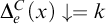 , contradicting the assumption that
$\Delta _e^{C}(x)\uparrow $
 .
Part (1) of the lemma says that, if at some stage s, we have
$\Delta _{e,s-1}^{C_s}(x)\downarrow \neq D_s(x)$
 , then we shall have
$\Phi _{e,s}^{A_{0,s}\oplus C_s}(x)\downarrow \neq D_s(x)$
 , so we achieve a disagreement at stage s.
$\boldsymbol {P}_{\boldsymbol {e}}$
 -strategy
: At stage s, we first check whether there is some x such that
$\Delta _{e,s-1}^{C_s}(x)\downarrow \neq D_s(x)$
 . If so, we stop. Otherwise, we start with
$x=0$
 and proceed one by one until we stop:
-
(P.1) If $x=s$
, we stop. -
(P.2) Otherwise, we perform the $P_e(x)$
-strategy:-
(P.2a) If Item (Px.1) applies, we stop.
-
(P.2b) Otherwise, if Item (Px.2) applies, we repeat with $x:=x+1$
. -
(P.2c) Otherwise, if Item (Px.3a) applies, we stop.
-
(P.2d) Otherwise, if Item (Px.3b) applies, then $P_e(x)$
acts and we also say that
$P_e$
acts; we impose a restraint on
$A_0\!\upharpoonright \! s$
and then stop.
-


As usual, we ensure that if
$P_e(x)$
 is injured at stage s for some x, then
$P_e$
 is initialized at the same stage.
Lemma 4.4. Suppose the
$P_e$
 -requirement is not initialized after
$s_0$
 . Then
$P_e$
 is satisfied. Moreover, there exists some stage
$s_2>s_0$
 after which
$P_e$
 does not act. The restraint imposed on
$A_0$
 is therefore bounded by
$s_2$
 .
Proof. Let
$\mathcal {B} = \{x\in \operatorname {\mathrm {dom}} \Delta _e^C\mid \Delta _e^C(x)\downarrow \neq D(x)\}$
 , which is a
$\Sigma _1^C$
 subset of M.
Case 1:
$\mathcal {B}=\varnothing $
 and
$\operatorname {\mathrm {dom}} \Delta _e^C=M$
 . In this case,
$D=\Delta _e^C$
 , contradicting
$D\nleq _{pT} C$
 .
Case 2:
$\mathcal {B}\neq \varnothing $
 or
$\operatorname {\mathrm {dom}} \Delta _e^C\neq M$
 . By
$\mathsf {L}\Sigma _1^C$
 , let a be the least element such that either
$\Delta _e^C(a)\downarrow \neq D(a)$
 or
$\Delta _e^C(a)\uparrow $
 . Then for each
$x<a$
 ,
$\Delta _e^C(x)\downarrow =D(x)$
 .
If
$a=0$
 , let
$s_1=0$
 .
If
$a>0$
 , let
$g:a\to M$
 be given by
$g(x)=s$
 if for some
$\sigma $
 with
$C\in [\sigma ]$
 ,
$\Delta _e^\sigma (x)$
 is defined at stage s. Since g is C-computable with M-finite domain,
$\operatorname {\mathrm {ran}} g$
 is bounded by some
$s_1$
 , by
$\mathsf {B}\Sigma _1^C$
 .
Then for all
$x<a$
 and all
$s>s_1$
 ,
$P_e(x)$
 does not act at stage s. For the
$P_e(a)$
 -subrequirement, Lemma 4.1 shows that there exists some
$s_2\ge s_1$
 after which
$P_e(a)$
 does not act. Lemma 4.3(2) and (3) shows that
$P_e$
 is satisfied. Moreover, at each stage
$s>s_2$
 , either Item (P.2a) or Item (P.2c) applies, so
$P_e$
 does not act at stage s.
This completes the proof.
4.3 Block of requirements
We take
$\Lambda $
 , a block of P-requirements, as an example; blocks of Q-requirements are similar. Assume
$\Lambda =\{P_{e_0}, P_{e_0+1}, \dots , P_{e_1}\}$
 . To simplify notation, we conflate
$\Lambda $
 with the index set
$\{e_0, e_0+1, \dots , e_1\}$
 . Each of the requirements in
$\Lambda $
 follows the
$P_e$
 -strategy, and they have no conflicts with each other. Now we shall prove the analogue of Lemma 3.2.
Lemma 4.5. Suppose there exists some
$s_0$
 after which no requirements in
$\Lambda $
 are initialized. Then all requirements in
$\Lambda $
 are satisfied, and there exists some
$s_3> s_0$
 after which no requirement in
$\Lambda $
 acts. Moreover, the restraint imposed on
$A_0$
 by
$\Lambda $
 is bounded by
$s_3$
 .
Proof. By Lemma 4.4, each
$P_e$
 with
$e\in \Lambda $
 is satisfied. It remains to show the existence of such an
$s_3$
 .
We define
$f:\Lambda \to M$
 by

where the x in the statement is not necessarily the least one. For such x and s, we also have
$D_s(x)=D(x)$
 since D is a c.e. set. Since f is a partial C-computable function,
$\operatorname {\mathrm {ran}} f$
 is bounded by some
$s_1$
 . That is, for each
$e\in \operatorname {\mathrm {dom}} f$
 and each stage
$s>s_1$
 ,
$P_e$
 does not act at stage s. Since
$\operatorname {\mathrm {dom}} f$
 is a
$\Sigma _1^C$
 subset of
$\Lambda $
 , it is M-finite. We let
$\Lambda _1 = \Lambda \setminus \operatorname {\mathrm {dom}} f$
 .
Then we claim that
$\bigcup _{e\in \Lambda _1} \operatorname {\mathrm {dom}} \Delta _e^C \neq M$
 . To see this, suppose otherwise that
$\bigcup _{e\in \Lambda _1} \operatorname {\mathrm {dom}} \Delta _e^C = M$
 . Then for all
$x\in M$
 and
$i\in \{0,1\}$
 ,

This shows that both D and
$\bar {D}$
 are
$\Sigma _1^C$
 , which implies
$D\le _{pT} C$
 , contradicting the assumption
$D\nleq _{pT} C$
 . Therefore, there exists
$b'\notin \bigcup _{e\in \Lambda _1} \operatorname {\mathrm {dom}} \Delta _e^C$
 . Let
$b=b'+1$
 so that for each
$e\in \Lambda _1$
 , there exists
$x < b$
 such that
$\Delta _e^C(x)\uparrow $
 .
Define
$g:\Lambda _1\times b\to M$
 by

So
$\operatorname {\mathrm {ran}} g$
 is bounded by some
$s_2$
 . This means that for each
$e\in \Lambda _1$
 and each
$x\in \operatorname {\mathrm {dom}} \Delta _e^C$
 with
$x<b$
 ,
$P_e(x)$
 does not act after stage
$s_2$
 .
Now for
$x<b$
 with
$x\notin \operatorname {\mathrm {dom}} \Delta _e^C$
 ,
$P_e(x)$
 may still act after
$s_2$
 several times. We would like to find a stage
$s_3$
 bounding the stages at which these subrequirements act.
To do this, let
$j_{e,x}$
 for
$e\in \Lambda _1$
 and
$x<b$
 be the index of the guessing set
$W_{j_{e,x}}$
 for the
$P_e(x)$
 -strategy. This mapping
$(e,x)\mapsto j_{e,x}$
 is computable.
Recall from the beginning of Section 4 that q is a computable function such that for each
$j\in M$
 ,

Now, the mapping
$(e,x)\mapsto q(j_{e,x})$
 with domain
$\Lambda _1\times b$
 is computable, and by
$\mathsf {B}\Sigma _1$
 , its range is bounded by some d. Then we define
$w:\Lambda _1\times b\times d\to M$
 by

Then,
$\mathsf {I}\Sigma _1$
 implies that
$\operatorname {\mathrm {ran}} w$
 is bounded by some
$s_3>s_2$
 . In particular, for each
$e\in \Lambda _1$
 and
$x<b$
 with
$x\notin \operatorname {\mathrm {dom}} \Delta _e^C$
 , we have
$p(j_{e,x},s)=0$
 at each stage
$s>s_3$
 , and therefore no computation will be certified in the
$P_e(x)$
 -strategy. Hence, these
$P_e(x)$
 do not act after stage
$s_3$
 .
Putting this together, we have shown that for each
$e\in \Lambda $
 and each stage
$s>s_3$
 ,
$P_e$
 does not act.
Dynamic priority assignments are the same as in Section 3.3, so we move directly to the construction and verification.
5 Discussion
We point out that the original Robinson Splitting Theorem can be proved in models of
$\mathsf {P}^-+\mathsf {B}\Sigma _2$
 . This is not surprising, since Groszek, Mytilinaios, and Slaman [Reference Groszek, Mytilinaios and Slaman8] showed that
$\mathsf {B}\Sigma _2$
 implies the Sacks Density Theorem. Recall that Chong and Yang [Reference Chong and Yang3] and Groszek, Mytilinaios, and Slaman [Reference Groszek, Mytilinaios and Slaman8] showed that in models of
$\mathsf {P}^-+\mathsf {B}\Sigma _2$
 , every incomplete c.e. set is hyperregular. Therefore, most of our proof applies to an arbitrary low set C. The only additional issue is that the proof of Lemma 4.5 in its current form also uses the fact that X is
$\omega $
 -c.e., where X is the set for Robinson’s trick. Under
$\mathsf {B}\Sigma _2$
 , however, this lemma has a much shorter proof. Define
$f:\Lambda \to M$
 by

This is a
$\Pi _1$
 function defined for each
$e\in \Lambda $
 (by Lemma 4.4), and
$\mathsf {B}\Pi _1$
 (equivalent to
$\mathsf {B}\Sigma _2$
 ) implies that
$\operatorname {\mathrm {ran}} f$
 is bounded. This yields Lemma 4.5. Note also that under
$\mathsf {B}\Sigma _2$
 ,
$\le _{pT}$
 is equivalent to
$\le _{sT}$
 for c.e. sets, which justifies the concept of c.e. degrees in such models. Hence we obtain the following theorem.
Theorem 5.1. The Robinson Splitting Theorem (Theorem 1.2) holds in models of
$\mathsf {P}^-+\mathsf {B}\Sigma _2$
 .
Note also that there is a saturated model
$M\models \mathsf {P}^-+\mathsf {B}\Sigma _2$
 in which all incomplete
$\Delta _2^0$
 sets are low [Reference Chong, Li and Yang1]. By Theorem 5.1, Lachlan’s Nonsplitting Theorem does not hold in this model.
Corollary 5.2.
$\mathsf {P}^-+\mathsf {B}\Sigma _2$
 does not prove Lachlan’s Nonsplitting Theorem.
We leave the following question open.
Question 5.3. Does
$\mathsf {I}\Sigma _1$
 prove the original Robinson Splitting Theorem when the set C is low? Or is it equivalent to
$\mathsf {B}\Sigma _2$
 over
$\mathsf {P}^-+\mathsf {I}\Sigma _1$
 ?
Our argument relies heavily on the fact that X and
$C'$
 are
$\omega $
 -c.e., which is a special case of the Ershov hierarchy. Heuristically, if a set A is easy to approximate, it is regular; if its jump is easy to approximate, it is hyperregular. We need hyperregularity of C and an easy approximation of X in the construction; this may suggest a deeper relation between hyperregularity from reverse recursion theory and the Ershov hierarchy from classical recursion theory. One may ask the following question.
Question 5.4. Let
$M\models \mathsf {P}^-+\mathsf {I}\Sigma _1$
 . What computable ordinal
$\alpha $
 guarantees that if
$A\subseteq M$
 is
$\alpha $
 -c.e., then A is regular in M?
In the standard model
$\mathbb {N}$
 , Faizrakhmanov [Reference Faizrakhmanov5] showed that if
$C'$
 is
$\alpha $
 -c.e. for some
$\omega \le \alpha <\omega ^2$
 , then
$C'$
 is
$\omega $
 -c.e. and hence regular. Whether his result holds in models of
$\mathsf {P}^-+\mathsf {I}\Sigma _1$
 is not known to us.
The study of the Robinson Splitting Theorem over
$\mathsf {I}\Sigma _1$
 may also be related to the following special case of the Sacks Density Theorem.
Question 5.5. Does
$\mathsf {I}\Sigma _1$
 prove the upper density property: For every c.e. degree
$C<_T K$
 , there exists a c.e. degree D such that
$C<_T D<_T K$
 ?
It would be unexpected if the upper density property already failed for low degrees C in some model of
$\mathsf {I}\Sigma _1$
 .
Acknowledgments
We thank the anonymous referee for carefully reading the article and for suggestions that improved its presentation, making it more accessible to a broader audience. We would also like to thank Yang Yue for valuable discussions and suggestions.
Funding
C.P.’s research was partially funded by the National Natural Science Foundation of China (Grant No. 12271264). M.S.’s work was supported by the National Science Centre, Poland (Grant No. 2023/49/B/ST1/02627).



