3. Results

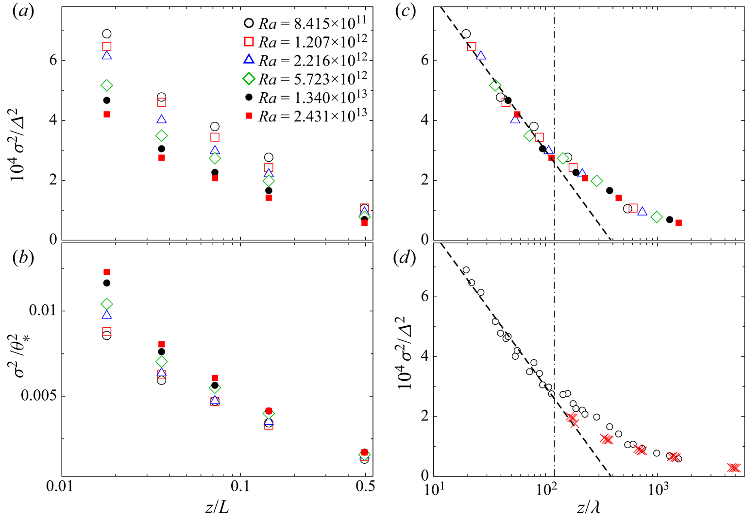
Figure 1 shows several typical sets of $\sigma ^2(z)$ data as a function of $z/L$ for $\varGamma = 0.50$. In figure 1(a,b), the variance data for $8\times 10^{11} \underset{\smash{\scriptscriptstyle\thicksim}} { < } Ra \underset{\smash{\scriptscriptstyle\thicksim}} { < } 2\times 10^{13}$ were scaled by $\varDelta ^2$ and $\theta _*^2$, respectively. Here $\theta _* = Q_0 / (Q_0\beta g L)^{1/3}$ with $Q_0 = \kappa Nu \varDelta / L$. This is a temperature scale for the mixing zone ($z/\lambda \underset{\smash{\scriptscriptstyle\thicksim}} { > } 5$ and $z/L \underset{\smash{\scriptscriptstyle\thicksim}} { < } 0.1$) proposed by Deardorff (Reference Deardorff1970). The plots show that neither $\sigma ^2/\varDelta ^2$ nor $\sigma ^2/\theta _*^2$ collapse onto a single (‘universal’) curve when plotted as a function of $z/L$.

Figure 1.

Fluctuation results for $\varGamma = 0.50$ at the radial location $\xi = 0.0357$. (a) $\sigma ^2(z)/\varDelta ^2$ and (b) $\sigma ^2(z)/\theta _*^2$ as a function of $z/L$ for several $Ra$. (c) $\sigma ^2(z)/\varDelta ^2$ as a function of $z/\lambda = (z/L)\times (2Nu)$. The data are the same as in (a). (d) $\sigma ^2(z)/\varDelta ^2$ for $Ra \underset{\smash{\scriptscriptstyle\thicksim}} { < } 2.5\times 10^{13}$ (black circles) and for $Ra \underset{\smash{\scriptscriptstyle\thicksim}} { > } 2\times 10^{14}$ (red crosses) as a function of $z/\lambda$. Here $Nu$ was simultaneously measured with the same sample in the classical state. The dashed lines in (c,d) represent the logarithmic function $\sigma ^2(z) / \varDelta ^2= M\times \ln (z/\lambda ) + N$.

In the mixing zone, where plumes accumulate above or below the thermal BL, local temperature fluctuations are dominated by thermal plumes rather than by turbulent background flow. As the thermal plumes have emanated from the temperature BLs, the plume region and the BLs can be expected to be characterized by the same scales. To test this idea, we used the BL thickness $\lambda$ as the length scale and $\varDelta$ as the temperature scale for our data. In figure 1(c), we plot the $\sigma ^2(z)/\varDelta ^2$ data shown in figure 1(a) as a function of $z/\lambda$. Here $\lambda = L/(2{Nu})$ with $Nu$ simultaneously measured with the same sample. Details of the $Nu$ measurements have been reported previously (Ahlers et al. Reference Ahlers, He, Funfschilling and Bodenschatz2012b; He et al. Reference He, Funfschilling, Nobach, Bodenschatz and Ahlers2012b), and the results showed ${Nu} = 0.1044Ra^{0.312}$ in the classical regime. It is found that the measured $\sigma ^2/\varDelta ^2$ for all $Ra$ collapse onto a universal curve over the whole range of $z/\lambda$. In figure 1(d), we added the variance data for $Ra \underset{\smash{\scriptscriptstyle\thicksim}} { > } 2 \times 10^{14}$ for comparison. For those data, the values of $\lambda$ were calculated using the extrapolation of the $Nu$ power law given above for the classical state. It is seen that the normalized variance profiles deviate from the collapsed curve for $Ra < Ra^*_1 \simeq 2 \times 10^{13}$, with deviations larger than experimental errors.

Previous experimental and numerical studies had found that some features of the temperature field in RBC behave in a manner analogous to those of the velocity in wall-bounded turbulence. For $z/\lambda \underset{\smash{\scriptscriptstyle\thicksim}} { > } 10$ and $z/L \underset{\smash{\scriptscriptstyle\thicksim}} { < } 0.1$ (the plume-dominated mixing region) the mean temperature $\langle T(z) \rangle$ follows a logarithmic profile (Ahlers et al. Reference Ahlers, Bodenschatz, Funfschilling, Grossmann, He, Lohse, Stevens and Verzicco2012a,  Reference Ahlers, Bodenschatz and He2014; van der Poel et al. Reference van der Poel, Ostilla-Mónico, Verzicco, Grossmann and Lohse2015). In the logarithmic layer the temperature frequency spectra $P(\,f\tau _0)$ have the universal $f^{-1}$ scaling $P(\,f\tau _0) = P_0\times (\,f\tau _0)^{-1}$ with $P_0 = 0.208$. Here $\tau _0 = \sqrt {2R_0}$ is the Taylor microscale in time, where $R_0$ is the radius of curvature of the temperature autocorrelation function at $\tau = 0$ (He et al. Reference He, van Gils, Bodenschatz and Ahlers2014). Far above the plate, near $z/L = 0.5$, the spectra closely follow $P(\,f\tau _0) \sim (\,f\tau _0)^{-1.67}$, consistent with the Obukhov–Corrsin scaling for passive scalars in fully developed turbulence (Obukhov Reference Obukhov1949; Corrsin Reference Corrsin1951). For velocity in shear-flow turbulence the logarithmic variation arises from eddies attached to the wall (Townsend Reference Townsend1976), while for the temperature in RBC it is due to thermal plumes emitted by the BL (Ahlers et al. Reference Ahlers, Bodenschatz and He2014; van der Poel et al. Reference van der Poel, Ostilla-Mónico, Verzicco, Grossmann and Lohse2015). It is reasonable to assume that plumes in RBC play a role similar to the eddies in shear-flow turbulence. With this assumption, we proposed a model for the temperature variance based on dimensional analysis in wavenumber space (He et al. Reference He, Bodenschatz and Ahlers2021), and derived the universal form

(3.1)\begin{equation} \sigma^2/\varDelta^2 = c_1\ln(z/\lambda) + c_2 + c_3 (z/\lambda)^{{-}0.5} \end{equation}

for $\sigma ^2$. Note that in (3.1) the predicted scaling function of $\sigma ^2$ is universal, but not the parameters. The parameters $c_1$, $c_2$ and $c_3$ can be adjusted so as to fit the data, but their relationships to other quantities are given by

(He et al. Reference He, Bodenschatz and Ahlers2021)

(3.2)$$\begin{gather} c_1 ={-}M_1 , \end{gather}$$

(3.3)$$\begin{gather}c_2 = N_1-M_1 \ln\left( \frac{Re_*}{2Nu}\right) \end{gather}$$

and

(3.4)\begin{equation} c_3 = C_1 \left( \frac{Pr Re_*}{2Nu} \right)^{{-}0.5} , \end{equation}

where $M_1$ and $C_1$ are universal constants, $N_1$ is a large-scale characteristic constant, the shear velocity $u_* \equiv \sqrt {\nu (\partial U/\partial z )\vert _{z=0}}$ and the Reynolds number $Re_*= u_*L/\nu$. In a confined RBC sample, we should of course expect the three parameters ($c_1$, $c_2$ and $c_3$) to depend on $r$ and $\varGamma$, and thus to be determined from experimental data. Note that when $Pr$ approaches infinite, the power-law term in (3.1) vanishes and the temperature variance will solely follow the logarithmic profile.

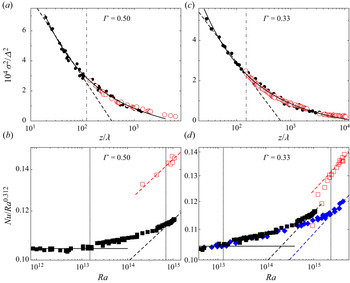
To test this model, we used (3.1) to fit the $\sigma ^2/\varDelta ^2$ data in the classical regime for $Ra \underset{\smash{\scriptscriptstyle\thicksim}} { < } 1.5 \times 10^{13}$ and $\varGamma = 0.50$. As shown in figure 2(a), the overlapped $\sigma ^2/\varDelta ^2$ data can be well described by the fitted curve over the whole range of $z/\lambda$, which corresponds to $z/L \underset{\smash{\scriptscriptstyle\thicksim}} { < } 0.5$ and thus covers essentially the entire sample. This fit indicates that the model captures the essential physics. In the range $20 \underset{\smash{\scriptscriptstyle\thicksim}} { < } z/\lambda \underset{\smash{\scriptscriptstyle\thicksim}} { < } 120$, which is the logarithmic layer for $\langle T(z) \rangle$ (Ahlers et al. Reference Ahlers, Bodenschatz and He2014), the variance data closely follow a logarithmic form as illustrated by the dashed line. It is noted that in the same range, a power function with adjustable parameters can fit the $\sigma ^2(z)/\varDelta ^2$ data almost equally well; however, neither a logarithmic nor a power function can fit the overlapped data over the whole range of $z/\lambda$ well above $1000$.

Figure 2.

Results for (a,c) $\sigma ^2/\varDelta ^2$ as a function of $z/\lambda$ and (b,d) the reduced $Nu/Ra^{0.312}$ as a function of $Ra$. Results in (a,b) are for $\varGamma = 0.50$ and in (c,d) are for $\varGamma = 0.33$. In (a) black filled circles represent the data for $Ra \underset{\smash{\scriptscriptstyle\thicksim}} { < } 2\times 10^{13}$ with $\lambda = L/(2Nu)$. The black line is the fit of (3.1) to the filled circles which gave $c_1 = -1.84\times 10^{-5}$, $c_2 = 1.24\times 10^{-4}$ and $c_3 = 2.75\times 10^{-3}$. Red open circles are for $Ra \underset{\smash{\scriptscriptstyle\thicksim}} { > } 2\times 10^{14}$ with $\lambda$ replaced by $\tilde {\lambda } = L/(2 \widetilde {Nu})$ with $\widetilde {Nu}$ adjusted to give the best fit to the solid line. In (c) black filled circles represent the variance data for $Ra \underset{\smash{\scriptscriptstyle\thicksim}} { < } 5.5 \times 10^{14}$. The solid line is the fit of (3.1) to the filled circles which gave $c_1 = -8.53\times 10^{-6}$, $c_2 = 6.09\times 10^{-5}$ and $c_3 = 2.56\times 10^{-3}$. Red open circles are for $Ra \underset{\smash{\scriptscriptstyle\thicksim}} { > } 10^{15}$ with $\lambda$ replaced by $\tilde {\lambda }$. In (b,d) black filled squares are the measured $Nu$ for $\varGamma = 0.50$, while the filled blue diamonds in (d) are the measured $Nu$ for $\varGamma = 0.33$. Red squares represent $\widetilde {Nu}$ obtained from the fit of the red open circles to the solid curves in (a,c). The horizontal lines represent the classical scaling $Nu = 0.1044Ra^{0.312}$. Two pairs of vertical dotted lines are at $Ra^*_1$ and $Ra^*_2$ (see table 1). The parallel dashed lines represent the ultimate effective scaling $Nu \propto Ra^{0.38}$ and are plotted so as to pass through the data for $Ra > Ra^*_2$.

For $Ra \underset{\smash{\scriptscriptstyle\thicksim}} { > } 2 \times 10^{14}$ (i.e. during the transition to and in the ultimate state) the data deviated from the common curve found at smaller $Ra$ as illustrated in figure 1(d). As shown by the open red circles in figure 2(a,c), these large-$Ra$ data could be brought onto the same curve by replacing $\lambda$ with $\tilde \lambda = L/(2 \widetilde {Nu})$ and adjusting $\widetilde {Nu}$. The resulting values of $\widetilde {Nu}$ are shown as open red squares in figure 2(b,d). Figure 2(b) shows $Nu/Ra^{0.312}$ (filled squares) as a function of $Ra$ for $\varGamma = 0.50$. For $Ra > Ra^*_2 \simeq 8\times 10^{14}$ one sees that both $Nu$ and $\widetilde {Nu}$ follow the predicted scaling $Nu\propto Ra^{0.38 \pm 0.02}$ for the ultimate state, but the $\widetilde {Nu}$ data are larger by a factor of 1.09 than those for $Nu$.

For $\varGamma = 0.33$ we found that the normalized temperature spectra $P(\,f\tau _0)$ in the logarithmic region have the same form as that for $\varGamma = 0.50$ (not shown). Thus our model for the temperature variance is expected to be valid also for $\varGamma = 0.33$. Figure 2(c) shows $\sigma ^2/\varDelta ^2$ as a function of $z/\lambda$ measured at the radial location $\xi = 0.0357$ for $\varGamma = 0.33$. Filled black circles represent the data for $9.8\times 10^{12} \underset{\smash{\scriptscriptstyle\thicksim}} { < } Ra \underset{\smash{\scriptscriptstyle\thicksim}} { < } 5.6 \times 10^{14}$. As expected, all the variance data fall onto a unique curve also for this $\varGamma$, and they are well described by (3.1). For large $Ra$, in the range $9.6\times 10^{14} \underset{\smash{\scriptscriptstyle\thicksim}} { < } Ra \underset{\smash{\scriptscriptstyle\thicksim}} { < } 4.5 \times 10^{15}$, the data did not fall onto the same curve and $\tilde {\lambda }$ with an adjustable $\widetilde {Nu}$ had to be used to achieve the fit shown by the open red circles in figure 2(c).

In figure 2(d) we show the results for $Nu$ (filled blue diamonds) and $\widetilde {Nu}$ (open red squares) for $\varGamma = 0.33$. For comparison we also added the measured $Nu$ for $\varGamma = 0.50$ shown already in figure 2(b) (filled black squares) to the same plot. Over the large range $10^{12} \underset{\smash{\scriptscriptstyle\thicksim}} { < } Ra \underset{\smash{\scriptscriptstyle\thicksim}} { < } 5\times 10^{14}$ the results of $Nu$ for both $\varGamma$ agree well with each other and reveal a gradual transition from the classical scaling (horizontal solid line) for $Ra < Ra^*_1 \simeq 1.3 \times 10^{13}$ towards the ultimate scaling. For $\varGamma = 0.33$ we found $Ra^*_2 \simeq 2.3 \times 10^{15}$, which is larger than that for $\varGamma = 0.50$ and leads to a larger range of the transition. For $Ra \underset{\smash{\scriptscriptstyle\thicksim}} { > } Ra^*_2$, both $Nu$ and $\widetilde {Nu}$ were found to follow the predicted ultimate scaling, with $\widetilde {Nu}$ larger than $Nu$ by a factor of 1.14.

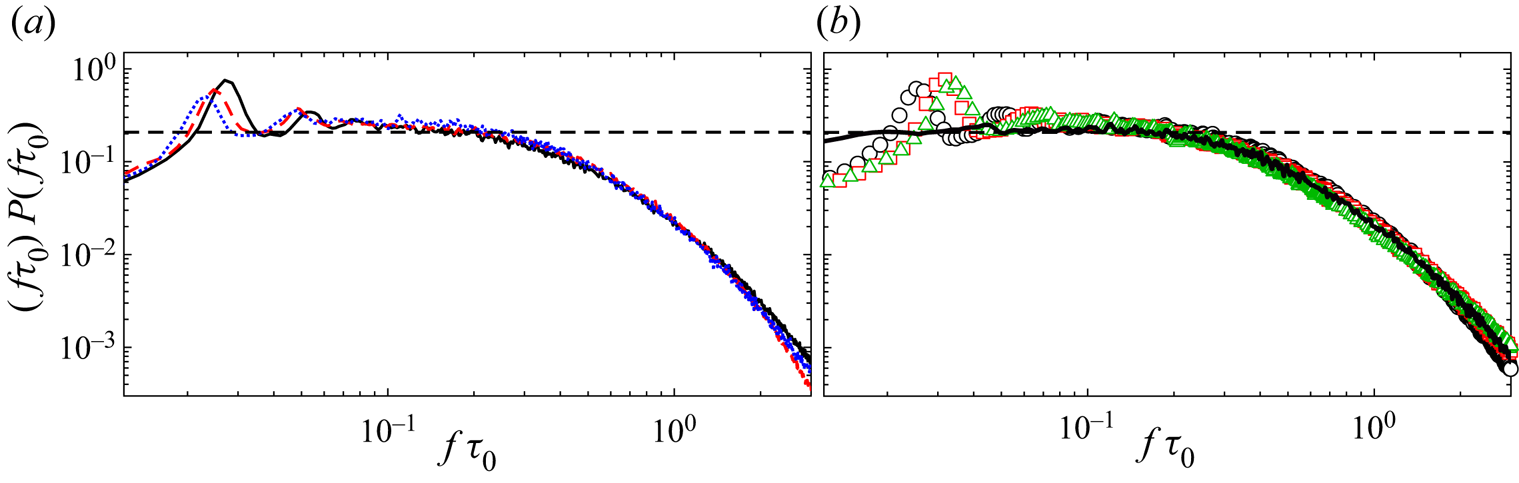
Next we turn to experimental results for $\varGamma = 1.00$. Figure 3(a) shows the compensated temperature spectra $(\,f\tau _0)P(\,f\tau _0)$ as a function of $f\tau _0$ measured in the logarithmic layer at the fixed height $z/L = 0.0357$ and $Ra = 1.35\times 10^{14}$ for different radial locations $\xi$. Figure 3(b) shows $(\,f\tau _0)P(\,f\tau _0)$ at the fixed height $z/L = 0.018$ and $\xi = 0.0196$ for several $Ra$. It is found that, within their uncertainty, all the spectra fall on the same curve and agree with the universal form measured previously (He et al. Reference He, van Gils, Bodenschatz and Ahlers2014) for $\varGamma = 0.50$ (black solid line in figure 3b), except for the peaks in the low-frequency part that change with measuring locations and $Ra$. Those peaks are attributed to periodic oscillations of the large-scale circulation (LSC) (see e.g. Qiu & Tong Reference Qiu and Tong2001; Funfschilling & Ahlers Reference Funfschilling and Ahlers2004; Brown & Ahlers Reference Brown and Ahlers2009; He, He & Tong Reference He, He and Tong2010; Wei & Ahlers Reference Wei and Ahlers2016) and contribute less than $10\,\%$ to the total power. The model discussed above does not consider the LSC contributions to the spectra.

Figure 3.

Reduced spectra $f\tau _0\times P(\,f\tau _0)$ as a function of $f\tau _0$ for $\varGamma = 1.00$. (a) $z/L = 0.037$ and $Ra = 1.35\times 10^{14}$ at radial locations $\xi = 0.268$ (blue dotted line), $0.064$ (black solid line) and $0.0196$ (red dashed line). (b) $z/L = 0.018$ and $\xi = 0.0106$ at $Ra = 1.35\times 10^{14}$ (black circles), $1.03 \times 10^{13}$ (red squares) and $3.38 \times 10^{12}$ (green triangles). The horizontal dashed lines correspond to $P(\,f\tau _0) = P_0 \times (\,f\tau _0)^{-1}$ with $P_0 = 0.208$. The black solid line in (b) is a typical spectrum for $\varGamma = 0.50$ measured at $z/L = 0.0179$, $\xi = 0.0178$ and $Ra = 1.08 \times 10^{15}$.

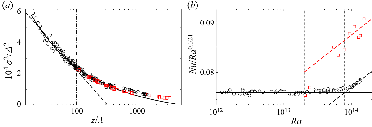
Figure 4(a) shows $\sigma ^2/\varDelta ^2$ as a function of $z/\lambda$ for $\xi = 0.0196$. Black circles represent the data for $Ra < Ra^*_1 \simeq 2\times 10^{13}$ with $\lambda$ calculated from the measured $Nu$. As seen in figure 2(a,c) for other $\varGamma$, the variance data for $\varGamma = 1.00$ also follow the predicted scaling form given by (3.1), but with slightly larger scatter. The scatter reflects the influence from the LSC dynamics on local temperature fluctuations. For $Ra > Ra_1^*$ we again replaced $Nu$ by $\widetilde {Nu}$ to calculate $\lambda$, and adjusted $\widetilde {Nu}$ so that all the variance data agreed with those for $Ra < Ra_1^*$. The results are shown by the red squares. In figure 4(b) we plot the reduced $\widetilde {Nu}/Ra^{0.312}$ (red squares) together with measured $Nu/Ra^{0.312}$ (black circles) data from He, Bodenschatz & Ahlers (Reference He, Bodenschatz and Ahlers2016) as a function of $Ra$. As $\varGamma$ increases, $Ra^*_1$ does not change much but $Ra^*_2$ decreases strongly, thus leading to a smaller transition range between $Ra_1^*$ and $Ra_2^*$. Above $Ra^*_2 \simeq 8\times 10^{13}$, we found that both $Nu$ and $\widetilde {Nu}$ scale as $Ra^{0.375 \pm 0.02}$, consistent with the predicted ultimate-state scaling but with $\widetilde {Nu}$ larger than $Nu$ by a factor of 1.13.

Figure 4.

Results for $\varGamma = 1.00$. (a) $\sigma ^2/\varDelta ^2$ as a function $z/\lambda$. Black circles: data for $Ra \underset{\smash{\scriptscriptstyle\thicksim}} { < } 2 \times 10^{13} \simeq Ra_2^*$ with $\lambda = L/(2Nu)$. The black solid line is the fit of (3.1) to the circles which gave $c_1 = -9.41\times 10^{-6}$, $c_2 = 4.70\times 10^{-5}$ and $c_3 = 2.42\times 10^{-3}$. Red open squares are for $Ra \underset{\smash{\scriptscriptstyle\thicksim}} { > } 2\times 10^{13}$ with $\lambda$ replaced by $\tilde {\lambda } = L/(2 \widetilde {Nu})$ and $\widetilde {Nu}$ adjusted to give the best agreement with the black circles. (b) $Nu/Ra^{0.321}$ as a function of $Ra$. Black circles: measured values. Red squares: $\widetilde {Nu}$ from the fit shown in (a). The vertical dotted lines are at $Ra_1^*$ and $Ra_2^*$. The parallel dashed lines represent the ultimate scaling $Nu \propto Ra^{0.375}$ and are plotted so as to pass through the data for $Ra > Ra^*_2$.

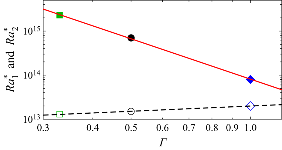
Finally, in figure 5, we summarize the results for the transition values $Ra_1^*$ and $Ra_2^*$ that were derived from the $Nu$ measurements. Some of these values were confirmed also by Reynolds number measurements (He et al. Reference He, Funfschilling, Nobach, Bodenschatz and Ahlers2012b,  Reference He, van Gils, Bodenschatz and Ahlers2015), measurements of logarithmic temperature profiles in the mixing layer (Ahlers et al. Reference Ahlers, Bodenschatz, Funfschilling, Grossmann, He, Lohse, Stevens and Verzicco2012a) and the azimuthal diffusivity of the LSC (He et al. Reference He, Bodenschatz and Ahlers2016). While there is a slight decrease of $Ra_1^*$ with decreasing $\varGamma$, $Ra_2^*$ increases strongly as $\varGamma$ decreases and is described well by $Ra_2^* = 8.1\times 10^{13} Ra^{-3.04}$. Thus, for small $\varGamma$ there is a relatively wide transition range, while this range apparently vanishes for $\varGamma$ just above one. A similar $\varGamma$ dependence $Ra^* \sim \varGamma ^{-2.5 \pm 0.5}$ was found in cryogenic experiments for $Pr \simeq 1.5$ over the range $0.23 \leq \varGamma \leq 1.14$ (Roche et al. Reference Roche, Gauthier, Kaiser and Salort2010; Roche Reference Roche2020). However, the values of $Ra^*$ (a transition Rayleigh number defined by the authors) are approximately $10^3$ times less than $Ra^*_2$. The destabilization of the ultimate state implied by the increase of $Ra_2^*$ as $\varGamma$ decreases can reasonably be attributed to the increasing length of the sidewalls which will tend to depress the turbulent flow in the bulk and thereby reduce the shear experienced by the BLs. It has been called to our attention (D. Lohse, personal communication) that a similar sidewall destabilization of convection occurs near onset where, for $\varGamma \underset{\smash{\scriptscriptstyle\thicksim}} { < } 1$, the critical Rayleigh number increases strongly with decreasing $\varGamma$ (Charlson & Sani Reference Charlson and Sani1971; Buell & Catton Reference Buell and Catton1983; Müller, Neumann & Weber Reference Müller, Neumann and Weber1984). We do not have an explanation for, and do not understand the origin of, the decrease of $Ra_1^*$ with decreasing $\varGamma$.

Figure 5.

The transition values $Ra^*_1$ (open symbols) and $Ra^*_2$ (filled symbols) of $Ra$ as a function of $\varGamma$. The black dashed line and red solid line represent the power laws $y = ax^b$ with the exponent $b = 0.40$ and $-3.04$, respectively.