

I. Introduction
The press and politicians often express the need for more precise and credible public firm information following financial turmoil and market failure, which they say will allow capital market participants to reduce information asymmetry and make better decisions. Notable examples of such legislative efforts include the Sarbanes–Oxley Act (2002) and the Dodd–Frank Act (2010). Despite the informational benefits these acts provide for capital market participants (Beyer, Cohen, Lys, and Walther (Reference Beyer, Cohen, Lys and Walther2010), Leuz and Wysocki (Reference Leuz and Wysocki2016)), the literature provides nuanced evidence on the economic consequences of disclosure regulations for firms. Studies find that mandating firms to disclose (or disseminate) more precise information can lead to inefficient investment decisions by discouraging investors’ private information production in stock prices and impeding managers’ ability to learn from stock prices (Jayaraman and Wu (Reference Jayaraman and Wu2019), Bird, Karolyi, Ruchti, and Truong (Reference Bird, Karolyi, Ruchti and Truong2021), and Goldstein, Yang, and Zuo (Reference Goldstein, Yang and Zuo2023)).Footnote 1 These studies suggest that regulators should consider both information benefits and real costs in evaluating mandatory disclosure regulation.
Our study extends this literature, which has focused on firm disclosures by examining how disclosures by financial intermediaries impact managerial learning from stock prices. Intermediaries provide useful information to capital market participants. For example, credit rating agencies (CRAs) inform both stock and bond investors about firms’ creditworthiness (Hand, Holthausen, and Leftwich (Reference Hand, Holthausen and Leftwich1992)). In the aftermath of high-profile bankruptcies, accounting scandals, and market failures, regulatory efforts to improve investor confidence about the precision and credibility of this kind of information (e.g., the Credit Rating Agency Reform Act) have arisen (e.g., Skreta and Veldkamp (Reference Skreta and Veldkamp2009), White (Reference White2010), and Goldstein and Yang (Reference Goldstein and Yang2019)). We contribute to the learning literature by examining the effect of the credibility of mandatory disclosure by CRAs on managerial learning from stock prices.
Our examination represents a joint test of the two propositions. First, we examine how the credibility of mandatory CRA disclosure influences stock price informativeness. Goldstein and Yang (Reference Goldstein and Yang2015) present a model in which informed traders facing multiple uncertainties specialize in analyzing a subset about which they have a comparative advantage but thus expose themselves to risks outside their specialization. Applying this model to our context, if CRA disclosure reveals information about a source of uncertainty that informed traders are less likely to specialize in, those traders will more actively acquire information about uncertainty that they are more likely to specialize in, enhancing stock price informativeness. Conversely, if CRA disclosure reveals information about a source of uncertainty that informed traders specialize in, they will scale back information acquisition, due to a reduction in their informational advantage over uninformed traders, leading to a decline in stock price informativeness.
Second, we explore how the credibility of mandatory CRA disclosure influences managerial learning from stock prices. The impact on learning depends on the type of investor information that CRA disclosure influences. If credit ratings reliably signal firm creditworthiness and investors tend to focus more on uncertainties, such as market demand and competition, then this shift in information acquisition increases managers’ reliance on stock prices. This increase occurs as informed traders have a greater competitive advantage in analyzing these uncertainties than do managers. However, if firms’ creditworthiness is difficult to assess due to uncertain consumer demand and industry competition, credit ratings will partially reveal information about these factors. This would then discourage investors from acquiring additional information about them and decrease managers’ dependence on prices. Taken together, depending on the type of investors’ private information that CRA disclosure is more likely to affect, managerial learning either increases or decreases.
To test these predictions, we choose the U.S. Credit Rating Agency Reform Act (CRARA) of 2006 as our setting. (See Section II.C for details.) Following several high-profile bankruptcies and the revelation of large-scale accounting fraud at Enron and WorldCom, major CRAs came under severe criticism, leading to regulatory and political scrutiny, including SEC reports and congressional and senate hearings. These events damaged the reputation of major CRAs as a reliable source of information on firms’ creditworthiness (Sethuraman (Reference Sethuraman2019)). In response, Congress passed CRARA on Sept. 29, 2006, to restore the reputation and enhance the accountability of CRAs.
Before testing our hypotheses, we validate our premise that CRARA improves the credibility of credit ratings. First, we find that the association between changes in firm fundamentals and subsequent changes in credit ratings strengthens after the passage of the law, suggesting that CRAs incorporate changes in firm fundamentals into their rating decisions more promptly post-CRARA. Importantly, stock market investors seem to perceive the improved credibility, as Sethuraman (Reference Sethuraman2019) documents that market reactions to changes in credit ratings increased after the law’s passage. We complement this evidence by examining the changes in financial reporting credibility. We follow Gipper, Leuz, and Maffett (Reference Gipper, Leuz and Maffett2020) and proxy for reporting credibility with stock market reactions to unexpected earnings news during short windows around earnings announcements (known as the earnings response coefficient or ERC). We find an increase in ERC after the passage of CRARA, suggesting that investors perceive the credibility of earnings as higher. Given that high-profile bankruptcies and accounting frauds prompted the passage of CRARA, these findings support the premise that the law improves the (perceived) credibility of credit ratings as a source of information about firm creditworthiness, particularly accounting fraud. Finally, we complement the above validation analyses by analyzing details of CRARA and provide institutional evidence consistent with this premise. (See Section II.C and Appendix A.)
Having established that CRARA improves the credibility of credit ratings as a source of information about firms’ creditworthiness, we examine the first part of our joint hypotheses. We use a difference-in-differences design with a sample of firms rated by major CRAs as the treatment group and unrated firms as the control group around the passage of CRARA. Using the probability of informed trading (PIN), price nonsynchronicity, and stock illiquidity as proxies for price informativeness, we find that stock price informativeness increases for firms affected by the act relative to control firms following its passage, suggesting that an increase in the credibility of mandatory CRA disclosure helps enhance stock price informativeness. This evidence suggests that investors acquire and trade more on information that they specialize in, presumably because they can obtain better information of firms’ creditworthiness post-CRARA.
Next, we turn to our second hypothesis regarding the effect of CRA disclosure credibility on managerial learning from stock prices. Following prior research (e.g., Bai, Philippon, and Savov (Reference Bai, Philippon and Savov2016)), we use the investment-price sensitivity framework. In a difference-in-differences design, we find an increase in investment-price sensitivity for treatment firms compared to control firms after CRARA. A parallel trends test shows no pre-trend in the investment-price sensitivity between treatment and control groups before the law’s passage. Overall, the results are consistent with managers relying more on stock prices to guide investment decisions after the law passed. We next explore within-treatment firm variation in the increase in investment-price sensitivity. We investigate how this increase is affected by i) types and dimensions of information that informed traders must gather and ii) the manager’s own information. The intuition for the first analysis is that informed traders’ information advantage lies in assessing growth opportunities and factors such as competition (e.g., Gao and Liang (Reference Gao and Liang2013), Jayaraman and Wu (Reference Jayaraman and Wu2019), Goldstein and Yang (Reference Goldstein and Yang2019), and Goldstein et al. (Reference Goldstein, Yang and Zuo2023)) and aggregating and synthesizing multiple dimensions of information (e.g., Goldstein and Yang (Reference Goldstein and Yang2015), (2019)). The intuition for the second analysis is that managers rely less on investor information when their own information is rich (e.g., Chen, Goldstein, and Jiang (Reference Chen, Goldstein and Jiang2007), Foucault and Frésard (Reference Foucault and Frésard2014), and Edmans, Jayaraman, and Schneemeier (Reference Edmans, Jayaraman and Schneemeier2017)). Consistent with these intuitions, we find that the increase in investment-price sensitivity strengthens when firms have greater growth opportunities, face more competition, have more segments, are exposed to greater risks, and when managers have poor information.Footnote 2
To further illuminate what type of uncertainty CRARA reduces, we investigate accounting fraud risk as a source of firm-specific uncertainty that informed traders face but that the law reduces. The reasoning is that the damaged reliability of credit ratings prior to CRARA mainly stems from investors’ concern about CRAs’ inability to detect accounting fraud. We find that CRARA seems to help mitigate this concern, evidenced by an increase in perceived reporting credibility. In response, investors may substitute the information production of factors potentially new to managers and opt out of assessing fraud risk in the post-CRARA era. Indeed, we find a more pronounced increase in investment-price sensitivity among firms with poor earnings quality (i.e., high risk of fraud) in the pre-CRARA era.
A concern is the possibility that an increase in investment-price sensitivity might reflect changes in the information possessed by investors. This would result in an increase in the alignment between managers’ and investors’ information, even though informed managers have not changed their investment policies. To address this concern, we examine the effect of CRARA on future firm performance. The intuition is that if the increase in investment-price sensitivity stems from increased learning by managers, we expect an increase in future firm performance. Using market-to-book and return on assets, we show that treatment firms do see better future performance. These results demonstrate improved efficiency and thus weigh against common information between the market and managers as an alternative explanation.
Another alternative explanation is that as credit rating agencies better monitor firms following CRARA, managers may make fewer self-dealing investments, such as empire-building, resulting in increased investment-price sensitivity. To address this concern, we conduct falsification tests and find that the increase in investment-price sensitivity does not vary with the strength of corporate governance.
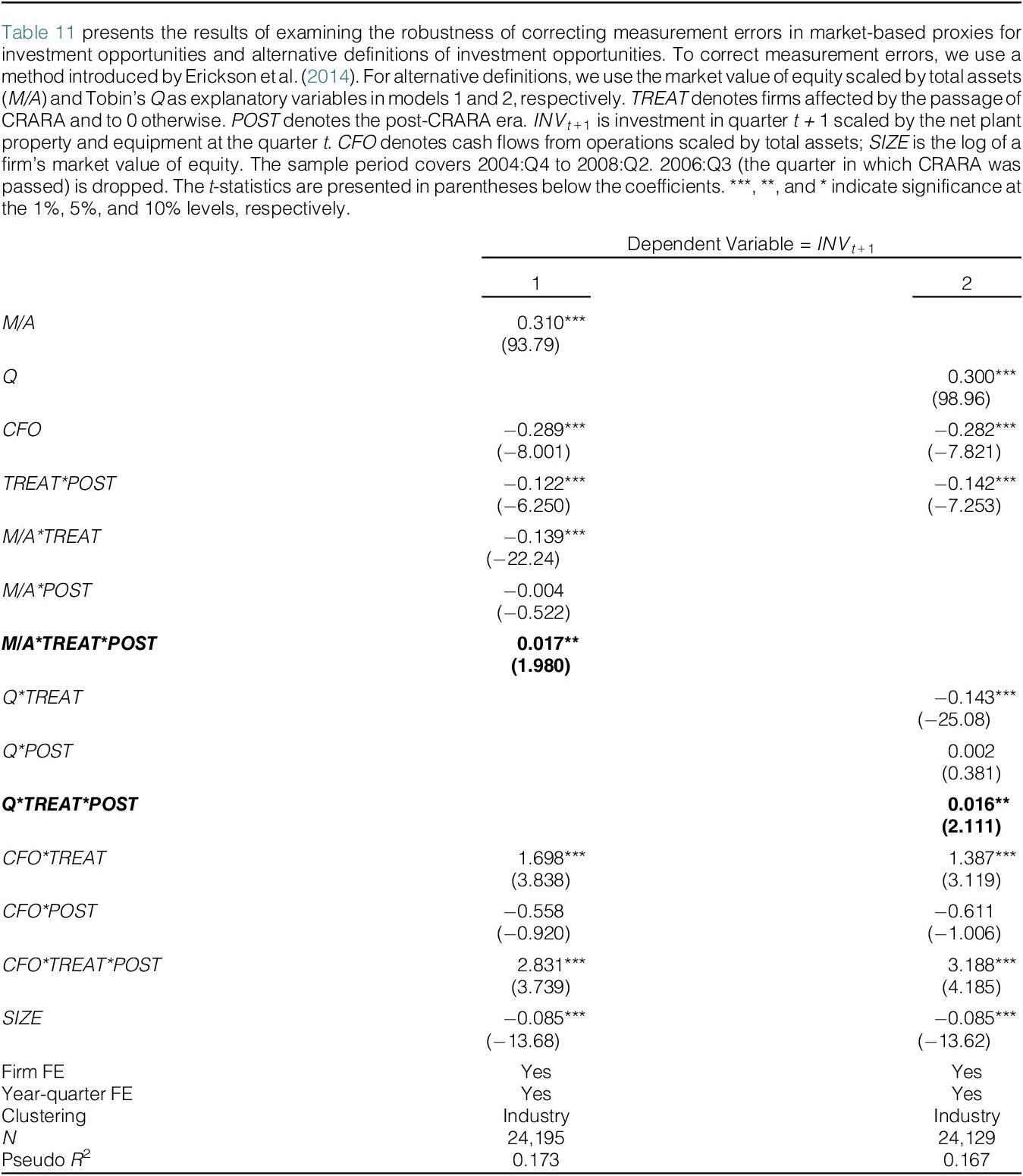
We also show the robustness of our results to alternative research designs. First, we use entropy balancing (e.g., Hainmueller (Reference Hainmueller2012)) and show that our main results hold. Next, we find our results robust to correcting measurement errors in proxies for investment opportunities (Erickson and Whited (Reference Erickson and Whited2000), (Reference Erickson and Whited2002), Erickson, Jiang, and Whited (Reference Erickson, Jiang and Whited2014), (Reference Erickson, Parham and Whited2017)) and alternative definitions of investment opportunities.
Our study makes two important contributions. First, we extend research on the effect of mandatory disclosure on managerial learning from stock prices. Studies primarily have examined how firms’ mandatory disclosures impact market-based feedback (e.g., Jayaraman and Wu (Reference Jayaraman and Wu2019), Bird et al. (Reference Bird, Karolyi, Ruchti and Truong2021), and Goldstein et al. (Reference Goldstein, Yang and Zuo2023)). In contrast, we examine how the credibility of mandatory disclosures from financial intermediaries, particularly CRAs, influences managerial learning. Our findings suggest that the credibility of mandatory disclosures by CRAs increases managerial learning from stock prices and thus firms’ investment efficiency. Our evidence is valuable for assessing the economic consequences of regulations designed to boost investors’ confidence in credit ratings and, more generally, regulatory efforts directed at public information provided by financial intermediaries (e.g., Skreta and Veldkamp (Reference Skreta and Veldkamp2009), White (Reference White2010), (Reference White2013), and Goldstein and Yang (Reference Goldstein and Yang2019)).
Our findings on the crowding-in effect of managerial learning from stock prices contrast with prior evidence of the adverse effects of mandatory firm disclosures and information dissemination, which have been shown to crowd out managerial learning from stock prices (e.g., Jayaraman and Wu (Reference Jayaraman and Wu2019), Bird et al. (Reference Bird, Karolyi, Ruchti and Truong2021), and Goldstein et al. (Reference Goldstein, Yang and Zuo2023)). This contrast highlights that the market feedback effects of mandatory disclosure depend on context, particularly the nature of the disclosure in question. In our study, mandatory CRA disclosure, by reliably signaling firm creditworthiness, motivates investors to acquire more information about such factors as market demand and competition. Since investors have a comparative advantage over managers in analyzing these factors, managerial learning from prices increases. Conversely, if mandatory disclosure provides better signals about market-wide factors, such as industry competition (segment disclosure in Jayaraman and Wu (Reference Jayaraman and Wu2019)), and thus reduces information advantage against unsophisticated investors, informed investors will reduce their acquisition of this information, resulting in a decrease in managerial learning from prices.
II. Related Literature, Hypothesis Development, and Setting
A. Related Literature
Our study contributes to the emerging literature that investigates the effects of mandatory disclosure on managerial learning from stock prices. Using the mandatory change to segment disclosures (SFAS 131), Jayaraman and Wu (Reference Jayaraman and Wu2019) find a decrease in investment-price sensitivity, with a more pronounced effect for firms with more informed trading and for financially unconstrained firms, consistent with mandatory disclosures reducing market feedback. Bird et al. (Reference Bird, Karolyi, Ruchti and Truong2021) and Goldstein et al. (Reference Goldstein, Yang and Zuo2023) explore the real effects of mandated dissemination of public information by using the staggered implementation of the SEC (Securities and Exchange Commission)’s EDGAR (Electronic Data Gathering, Analysis, and Retrieval) system. They find a decrease in investment-price sensitivity after EDGAR’s implementation, particularly when investors have an information advantage, consistent with price-based learning. By focusing on mandatory dissemination as opposed to disclosure, the two studies’ findings point to a similar conclusion that reducing informed traders’ information advantage via more timely dissemination of public information impedes managerial learning from stock prices.
Our study extends this line of research by focusing on mandatory disclosures from CRAs, rather than firms themselves, and by examining how the credibility of these mandatory disclosures, beyond disclosures alone, influences firm investment efficiency through managerial learning.
B. Hypothesis Development
Our analyses represent a joint test of the two hypotheses: i) how the credibility of mandatory CRA disclosure affects stock price informativeness and ii) whether the credibility of mandatory CRA disclosure influences managerial learning from stock prices.
Theory predicts that the effect of the credibility of mandatory CRA disclosure on stock price informativeness depends upon how the source of the disclosure is correlated with that of investors’ private information. Goldstein and Yang (Reference Goldstein and Yang2015) present a theoretical framework that suggests a favorable impact of mandatory CRA disclosure on stock price informativeness. In their model, informed traders encounter various uncertainties and thus focus on analyzing specific subsets of uncertainties. However, this specialization exposes those traders to risks associated with uncertainties outside their expertise. The model suggests that, as the cost of obtaining information about one source of uncertainty that informed traders do not specialize in decreases, they are more likely to acquire additional private information about another source of uncertainty, increasing stock price informativeness.Footnote 3
If, however, CRA disclosure partially reveals information about uncertainty that informed traders specialize in, that could decrease stock price informativeness. In this situation, CRA disclosure reduces informed traders’ information advantage against uninformed traders, and hence informed traders will scale back their information acquisition. Consistent with this prediction, Gao and Liang (Reference Gao and Liang2013) present a model where firm value is subject to two sources of uncertainties (assets-in-place and growth options), and these two sources are positively correlated. They predict that mandatory disclosure of assets-in-place discourages informed traders’ information acquisition about growth opportunities because this disclosure decreases informed traders’ information advantage about these opportunities. Given competing forces, we present our first hypothesis associated with stock price informativeness in two alternative forms:
Hypothesis 1a (price informativeness). The credibility of mandatory disclosure by CRAs increases stock price informativeness.
Hypothesis 1b (price informativeness). The credibility of mandatory disclosure by CRAs decreases stock price informativeness.
Learning theories posit that, while managers are arguably the most informed economic agents about sources of uncertainty that drive firm value, they are not perfectly informed about all sources and thus wish to learn from outsiders (Chen et al. (Reference Chen, Goldstein and Jiang2007), Gao and Liang (Reference Gao and Liang2013), Bai et al. (Reference Bai, Philippon and Savov2016), and Goldstein and Yang (Reference Goldstein and Yang2019)). The literature generally views firm-specific information, such as product quality, technology, and idiosyncratic creditworthiness, as well known to managers, whereas they aim to learn about industry distress risk, competition, and economy-wide factors—including macroeconomic conditions and economic policy uncertainty—from the market (e.g., Goldstein and Yang (Reference Goldstein and Yang2019)).
We argue that the effect of the credibility of mandatory CRA disclosure on managerial learning from stock prices depends on what types of investor information in stock prices are crowded out or crowded in by CRA disclosure, as hypothesized above. If credit ratings credibly signal firm-specific creditworthiness (i.e., lower cost of information acquisition) and reduce the uncertainty risk-averse traders face, investors are likely to acquire and trade on more information about such uncertainties as market demand and competition, in line with Hypothesis 1a. Since managers know about their own creditworthiness but less about market demand and competition, this substitution between these two types of information in stock prices will increase managerial learning from stock prices.
Note, however, that mandatory CRA disclosure could reduce managerial learning. For instance, if a firm’s creditworthiness is difficult to evaluate due to uncertain consumer demand and steeper competition, credible credit ratings not only reliably signal a firm’s creditworthiness but also partially reveal information about market demand and industry competition. Consequently, investors acquire less information about these uncertainties, as in Hypothesis 1b. To the extent that consumer demand and tougher competition are information that managers wish to learn from the market, their learning from stock prices decreases with more credible CRA disclosure. Given competing predictions, we present two alternative hypotheses:
Hypothesis 2a (managerial learning). Managerial learning from stock prices increases with the credibility of mandatory disclosure by CRAs.
Hypothesis 2b (managerial learning). Managerial learning from stock prices decreases with the credibility of mandatory disclosure by CRAs.
C. Experimental Setting: The Credit Ratings Agency Reform Act of 2006
CRAs are viewed as gatekeepers in capital markets in that they provide opinions on the creditworthiness of firms. Standard and Poor’s states: “Our ratings express the agency’s opinion about the ability and willingness of an issuer, such as a corporation or state or city government, to meet its financial obligations in full and on time.”
The role of CRAs as gatekeepers was called into question by high-profile accounting frauds in 2002 (e.g., the Enron scandal). Pundits pointed to inaccurate, untimely credit ratings as a contributor to the Enron crisis and called for better regulation (Coskun (Reference Coskun2008), Skreta and Veldkamp (Reference Skreta and Veldkamp2009)). Subsequently, an SEC investigation and congressional and senate hearings pointed out that CRAs ignored fundamental problems, like questionable transactions in 10-Ks and suspect accounting, in determining ratings due to conflicts of interest (Coskun (Reference Coskun2008)). The reputation of major CRAs was damaged. This situation led to the passage of the Credit Rating Agency Reform Act (CRARA) in 2006.
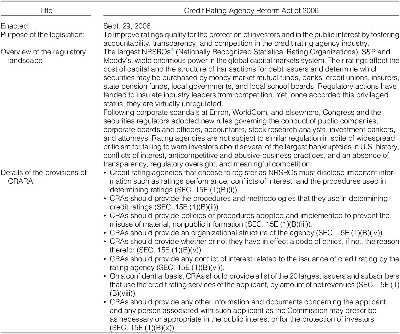
CRARA aimed to restore the reputation of CRAs rather than require more disclosures by them, and thus the law serves as an effective setting in which the credibility of firms’ credit ratings increases. CRARA was designed to i) bolster the accountability of CRAs, ii) ensure that sufficient information about the inputs to the rating process is available to the SEC and the public, and iii) increase competition among CRAs.
Our premise is that CRARA, on average, improves the credibility of credit ratings as a source of information about firms’ creditworthiness. To assess the plausibility of this premise, we provide both institutional and empirical evidence on each of the two elements of this presumed mechanism.
We conduct institutional analysis concerning the premise that the credibility of credit ratings as a source of firms’ creditworthiness increases after the act. Appendix A describes details of the provisions under CRARA. We argue that the provisions associated with the first two objectives will improve the rating credibility perceived by investors. First, the provisions mandating that CRAs disclose conflicts of interest in advance reduce the likelihood that they will inflate ratings or delay downgrades. Policies and procedures that prevent CRAs from misusing material nonpublic information also serve to proactively discipline CRAs. The provisions that are designed to enhance ratings transparency also discipline CRAs, as details about their procedures and methodologies allow sophisticated investors to assess the credibility of ratings—something infeasible without these disclosures. However, the provisions associated with increasing competition have an unclear impact because the dominance of the three big CRAs did not significantly change after the act’s passage. Consequently, we argue that the provisions of the act, on average, restore the credibility of CRAs as a reliable signal of creditworthiness. We provide empirical evidence consistent with this conclusion based on institutional analysis in Section IV.A.
III. Sample and Data Sources
To construct our sample, we obtain data from several sources: firms’ accounting information and Standard & Poor’s senior debt ratings from Compustat, stock price and return data from CRSP, and probability of informed trading data from Brown and Hillegeist (Reference Brown and Hillegeist2007). Our sample covers the period surrounding the passage of CRARA and comprises firm-quarters between Oct. 1, 2004, and June 30, 2008. We drop the third quarter of 2006, the quarter in which CRARA became law (Sept. 29, 2006). This leads to 7 quarters each for both the pre- and post-CRARA periods. Our sample ends in the second quarter of 2008 to avoid the effects of the Great Recession of 2008. We exclude all firms that belong to the financial and utility industries (SIC codes 6000–6999 and 4900–4999), which leaves 49,701 firm-quarter observations. Further, we delete observations without the necessary information to calculate variables for our analyses, leading to a sample of 24,344 firm-quarter observations (2,632 firms). Sample size also varies across cross-sectional tests due to the availability of data for partitioning variables.
IV. Research Design and Results
A. Validation Tests of CRARA
We begin by examining whether CRARA improves the credibility of credit ratings as a source of firms’ creditworthiness. In our analysis, we take a “market-based approach” by evaluating the overall effects of CRARA relative to the prior regime rather than by separately assessing the impact of specific provisions.
First, we follow prior research (Ayers, Laplante, and McGuire (Reference Ayers, Laplante and McGuire2010)) and examine the extent to which changes in firm fundamentals are associated with subsequent changes in credit ratings. The motivation for this analysis is that if CRARA enhances the accountability of CRAs, changes in firm fundamentals prefigure changes in credit ratings after the law’s passage. Credit rating letters span from AAA (indicating a strong capacity to pay interest and repay principal) to D (indicating actual default). We translate rating letters into numbers ranging from 21 to 1, where higher numbers indicate better ratings. Since it takes time for credit ratings to reflect changes in firm fundamentals, we measure changes in numerical credit ratings over various time horizons. This analysis is conducted only for firms with credit ratings.
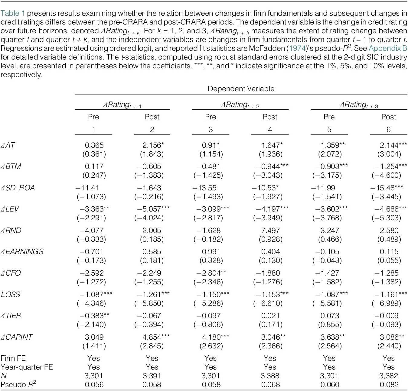
4We present the results of estimating ordered logistic regressions, separately for the pre- and post-CRARA periods in Table 1. ΔRATINGt + k denotes changes in Standard & Poor’s long-term issuer credit ratings in quarter t + k, where k is 1 through 3 as of quarter t. Following Bongaerts, Cremers, and Goetzman (Reference Bongaerts, Cremers and Goetzman2012), we present McFadden’s (Reference McFadden and Zarembka1974) pseudo-R 2 for each regression at the bottom of Table 1. Across three different horizons, the pseudo R 2s for the post-CRARA period exceed those for the pre-period. Furthermore, the differences between the pre- and post-CRARA periods increase with the length of windows for measuring changes in credit ratings. These results are consistent with CRAs incorporating changes in firm fundamentals into credit ratings more promptly after CRARA.

TABLE 1 Long description
The table presents regression results for three dependent variables: Delta Rating t plus 1, Delta Rating t plus 2, and Delta Rating t plus 3. Each is divided into Pre and Post columns numbered 1 through 6.
Key independent variables and their coefficients include:
* Delta A T: Shows a significant increase in the Post period for t plus 1 (2.156) and t plus 3 (2.144).
* Delta B T M: Shows significant negative coefficients in the Post periods for t plus 2 (-0.944) and t plus 3 (-1.254).
* Delta S D underscore R O A: Significant negative coefficient in the Post period for t plus 3 (-15.48).
* Delta L E V: Consistently negative and significant across all periods, with stronger coefficients in the Post columns (e.g., -5.057 in column 2 vs -3.363 in column 1).
* L O S S: Highly significant negative coefficients across all columns, ranging from -1.087 to -1.261.
* Delta C A P I N T: Significant positive coefficients in most columns, particularly in the Post periods.
Fixed Effects (F E) for Firm and Year-quarter are included (Yes) for all models. The sample size N is approximately 3,300 for all columns. Pseudo R-squared values range from 0.056 to 0.082, generally increasing from Pre to Post periods.
Next, we investigate whether investors perceive the quality of credit ratings as higher after the passage of CRARA. To this end, we examine changes in financial reporting credibility. Our analysis is motivated by the notion that, because investors previously questioned the reliability of credit ratings in assessing firm creditworthiness, especially due to CRAs’ failures to detect major accounting frauds, investors would place greater credibility on reported earnings if CRARA has indeed enhanced credit rating quality, as documented above. Following Gipper, Leuz, and Maffett (Reference Gipper, Leuz and Maffett2020), we proxy for reporting credibility with earnings response coefficients (ERC), measured as stock market reactions to unexpected earnings news during short windows around earnings announcements.
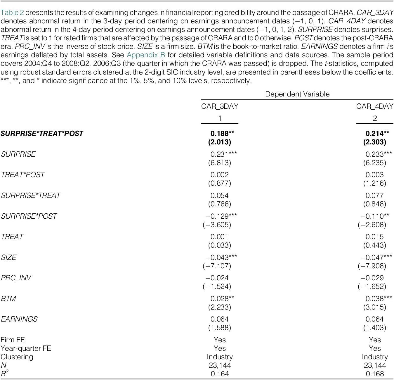
We present the results in Table 2. CAR_3DAY (CAR_4DAY) is cumulative abnormal return in the 3 days (4 days) centering on quarterly earnings announcements (−1, 0, 1) [(−1, 0, 1, 2)] (relative to a market model-adjusted benchmark, measured as the log of 1 plus actual return minus the log of 1 plus expected return (estimated using market models) on a day). SURPRISE is earnings surprise, measured as the difference between actual earnings minus mean analyst consensus earnings forecasts immediately preceding the actual earnings announcement, scaled by the stock price at the end of the prior quarter. As evidenced by the positive and significant coefficients on SURPRISE*TREAT*POST (p-value < 0.05), ERC increases incrementally among treatment firms after the passage of CRARA, indicating that investors seem to place higher weight on earnings surprises after CRARA. We interpret an increase in ERC among treatment firms as evidence of the law improving the perceived credibility of credit ratings as a source of information about firms’ creditworthiness.

TABLE 2 Long description
The table presents regression results for two dependent variables: C A R _ 3 D A Y in column 1 and C A R _ 4 D A Y in column 2.
Key variables and their coefficients (with t-statistics in brackets) are:
* S U R P R I S E asterisk T R E A T asterisk P O S T: 0.188 (2.013) in column 1; 0.214 (2.303) in column 2.
* S U R P R I S E: 0.231 (6.813) in column 1; 0.233 (6.235) in column 2.
* T R E A T asterisk P O S T: 0.002 (0.877) in column 1; 0.003 (1.216) in column 2.
* S U R P R I S E asterisk T R E A T: 0.054 (0.766) in column 1; 0.077 (0.848) in column 2.
* S U R P R I S E asterisk P O S T: minus 0.129 (minus 3.605) in column 1; minus 0.110 (minus 2.608) in column 2.
* T R E A T: 0.001 (0.033) in column 1; 0.015 (0.443) in column 2.
* S I Z E: minus 0.043 (minus 7.107) in column 1; minus 0.047 (minus 7.908) in column 2.
* P R C _ I N V: minus 0.024 (minus 1.524) in column 1; minus 0.029 (minus 1.652) in column 2.
* B T M: 0.028 (2.233) in column 1; 0.038 (3.015) in column 2.
* E A R N I N G S: 0.064 (1.588) in column 1; 0.064 (1.403) in column 2.
Fixed effects and controls:
* Firm F E: Yes for both.
* Year-quarter F E: Yes for both.
* Clustering: Industry for both.
* N: 23,144 for both.
* R-squared: 0.164 in column 1; 0.168 in column 2.
B. Effect of CRARA on Stock Price Informativeness (Hypothesis 1)
Having established that the credibility of credit ratings increases, we examine our first hypothesis by comparing changes in stock price informativeness before and after the passage of CRARA for the treatment group, relative to the control group. Specifically, we estimate the following difference-in-differences models (firm subscripts omitted):

where PRC_INFt represents proxies for stock price informativeness, as described in the following paragraph. TREAT is set equal to 1 for treatment firms and 0 otherwise. We categorize a firm as a treatment firm if it is rated by Standard & Poor’s, a major rating agency impacted by CRARA, and as a control firm if it is not rated by Standard & Poor’s.Footnote 4 POST is set equal to 1 for the quarters after CRARA and 0 otherwise (i.e., 7 quarters in the pre- and post-periods). We follow Jayaraman and Wu (Reference Jayaraman and Wu2019) and include firm size (SIZE) and the inverse of stock price (PRC_INV) as controls. We provide detailed variable definitions in Appendix B. We include firm (γ) and year-quarter (δ) fixed effects, which absorb the effect of TREAT and POST, respectively. We follow Jayaraman and Wu (Reference Jayaraman and Wu2019) and cluster standard errors by industry. A positive (negative) coefficient on β 1 will indicate that CRARA increases (decreases) stock price informativeness for affected firms compared to unaffected ones.
We follow Ferreira, Ferreira, and Raposo (Reference Ferreira, Ferreira and Raposo2011) and use the probability of informed trading (PIN) as our primary measure of price informativeness. This measure is derived from a structural market microstructure model, which posits that trades are executed by either noise traders or informed traders. However, empirical proxies that are based on structural models and use order flow data, such as PIN, have been subject to criticism. Collin-Dufresne and Fos (Reference Collin-Dufresne and Fos2016) suggest that strategic trading choices may limit the ability of these models to identify informed trading. Duarte, Hu, and Young (Reference Duarte, Hu and Young2021) find that these models do not match the moments of order flow observed in the data and lead to incorrect inferences about the presence of private information. Therefore, we use alternative price informativeness variables to corroborate our interpretation of the results. Following prior studies (Chen et al. (Reference Chen, Goldstein and Jiang2007), Jayaraman and Wu (Reference Jayaraman and Wu2019)), we employ stock price nonsynchronicity and Amihud’s (Reference Amihud2002) illiquidity measure.
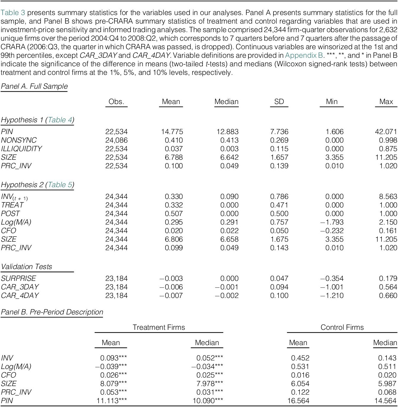
Panel A of Table 3 presents the descriptive statistics of the stock price informativeness sample. Means and medians of the three measures of price informativeness are generally consistent with those of prior studies (Morck, Yeung, and Yu (Reference Morck, Yeung and Yu2000), Durnev, Morck, Yeung, and Zarowin (Reference Durnev, Morck, Yeung and Zarowin2003), Chen et al. (Reference Chen, Goldstein and Jiang2007), Jayaraman and Wu (Reference Jayaraman and Wu2019), and Goldstein et al. (Reference Goldstein, Yang and Zuo2023)).

TABLE 3 Long description
Panel A, titled Full Sample, lists statistics for three categories.
1. Hypothesis 1 variables: P I N (Mean 14.775, Median 12.883), N O N S Y N C (Mean 0.410, Median 0.413), I L L I Q U I D I T Y (Mean 0.037, Median 0.003), S I Z E (Mean 6.788, Median 6.642), and P R C underscore I N V (Mean 0.100, Median 0.049).
2. Hypothesis 2 variables: I N V sub (t plus 1) (Mean 0.330, Median 0.090), T R E A T (Mean 0.332, Median 0.000), P O S T (Mean 0.507, Median 0.000), Log(M/A) (Mean 0.295, Median 0.291), C F O (Mean 0.020, Median 0.022), S I Z E (Mean 6.806, Median 6.658), and P R C underscore I N V (Mean 0.099, Median 0.049).
3. Validation Tests: S U R P R I S E (Mean minus 0.003), C A R underscore 3 D A Y (Mean minus 0.006), and C A R underscore 4 D A Y (Mean minus 0.007).
Panel B, titled Pre-Period Description, compares Treatment Firms and Control Firms across six variables.
1. I N V: Treatment Mean 0.093, Control Mean 0.452.
2. Log(M/A): Treatment Mean minus 0.039, Control Mean 0.531.
3. C F O: Treatment Mean 0.026, Control Mean 0.016.
4. S I Z E: Treatment Mean 8.079, Control Mean 6.054.
5. P R C underscore I N V: Treatment Mean 0.053, Control Mean 0.122.
6. P I N: Treatment Mean 11.113, Control Mean 16.564.
Asterisks in Panel B indicate statistical significance for the treatment group.
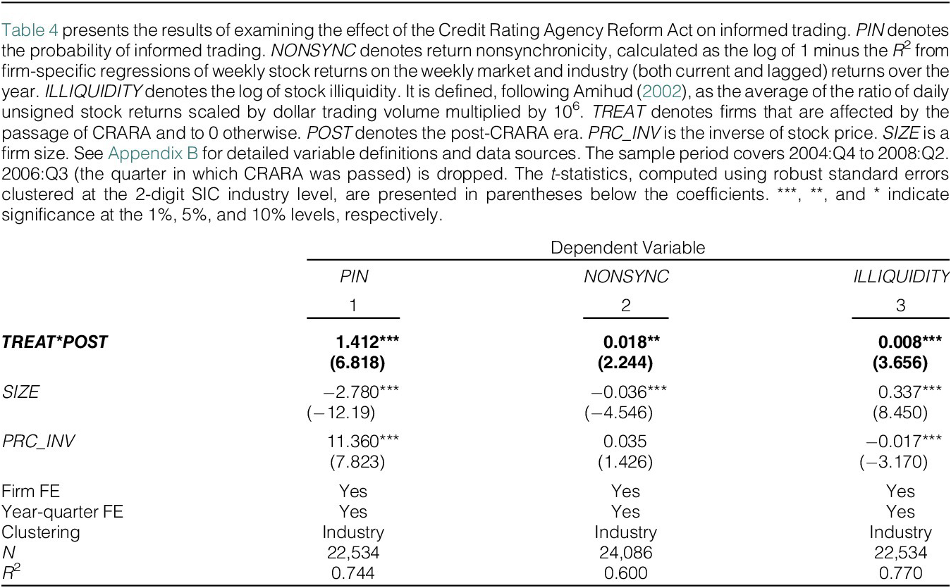
Table 4 reports the results. In model 1, we find a positive coefficient (p-value < 0.01) on TREAT*POST, indicating an increase in the probability of informed trading among firms affected by the passage of CRARA compared to unaffected firms. The results from alternative measures of stock price informativeness proxies provide similar inferences. In model 2, a significant coefficient of 0.018 indicates an increase in stock price nonsynchronicity, suggesting that stock returns co-move less after the passage of CRARA. Furthermore, a significant coefficient of 0.008 indicates a significant increase in the Amihud (Reference Amihud2002) measure after CRARA. Taken together, to the extent that our measures capture stock price informativeness, the results in Table 4 provide support for the hypothesis that the credibility of mandatory disclosure by CRAs increases stock price informativeness (Hypothesis 1a).Footnote 5

TABLE 4 Long description
The table consists of three numbered columns representing different regression models. The dependent variables are P I N for column 1, N O N S Y N C for column 2, and I L L I Q U I D I T Y for column 3.
Key results for the main interaction term T R E A T asterisk P O S T are as follows:
- Column 1 P I N: 1.412 with a t-stat of 6.818, significant at the 1 percent level.
- Column 2 N O N S Y N C: 0.018 with a t-stat of 2.244, significant at the 5 percent level.
- Column 3 I L L I Q U I D I T Y: 0.008 with a t-stat of 3.656, significant at the 1 percent level.
Control variables include:
- S I Z E: -2.780 t-stat -12.19 in column 1; -0.036 t-stat -4.546 in column 2; 0.337 t-stat 8.450 in column 3.
- P R C underscore I N V: 11.360 t-stat 7.823 in column 1; 0.035 t-stat 1.426 in column 2; -0.017 t-stat -3.170 in column 3.
Model specifications for all three columns include Firm F E, Year-quarter F E, and Industry clustering.
Summary statistics:
- Observations N: 22,534 for columns 1 and 3; 24,086 for column 2.
- R-squared: 0.744 for column 1; 0.600 for column 2; 0.770 for column 3.
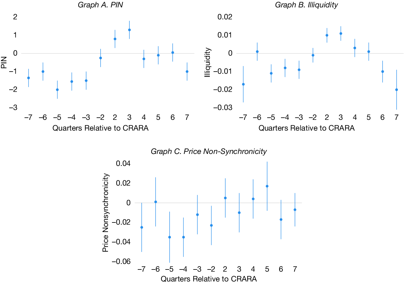
The parallel trends assumption is key to the identification of the effect of the disclosure regulation change (i.e., CRARA) on stock price informativeness in a difference-in-differences design (Roberts and Whited (Reference Roberts and Whited2013)). Although formally testing this assumption is infeasible, we take the advice of Roberts and Whited (Reference Roberts and Whited2013) and evaluate trends in stock price informativeness around the passage of CRARA.
We define a series of indicator variables equal to 1 for each quarter surrounding the passage of CRARA. We do not include indicators denoting quarter −1 and + 1, and they serve as the benchmark. In Figure 1, we plot the 12 coefficient estimates along with 95% confidence intervals to facilitate visual inspection. Differences in stock price informativeness appear to have increased immediately following the passage of CRARA, particularly in Graphs A and B of Figure 1.
Figure 1 shows difference-in-differences coefficients on price informativeness for each event-time. In Graphs A–C, the measures of price informativeness are PIN, illiquidity, and price nonsynchronicity, respectively. We define QTR(−7) as an indicator variable equal to 1 for observations in the 7 quarters before CRARA and 0 otherwise. The remaining indicators are defined analogously. QTR(−1) and QTR(+1) are omitted, serving as the benchmark. The dots (lines) represent coefficient estimates (95% confidence intervals).

FIGURE 1 Long description
A multi-panel figure with three graphs arranged in two rows. All graphs share a common x-axis labeled Quarters Relative to C R A R A, with discrete points at minus 7, minus 6, minus 5, minus 4, minus 3, minus 2, 2, 3, 4, 5, 6, and 7. A horizontal reference line is at zero.
Graph A, titled P I N, is at the top left. The y-axis ranges from minus 3 to 2. Data points show coefficients below zero from quarters minus 7 to minus 2, with a trough at minus 5. After the event, coefficients rise above zero at quarters 2 and 3 before returning toward zero and dipping at quarter 7.
Graph B, titled Illiquidity, is at the top right. The y-axis ranges from minus 0.03 to 0.02. Coefficients are generally negative before the event, particularly at quarter minus 7. Post-event, coefficients at quarters 2 and 3 are positive and statistically significant, followed by a decline back into negative territory by quarters 6 and 7.
Graph C, titled Price Non-Synchronicity, is centered on the bottom row. The y-axis ranges from minus 0.06 to 0.04. The data points exhibit high volatility with large vertical error bars representing 95 percent confidence intervals. Most points fluctuate around or below the zero line, with a notable positive peak at quarter 5.
C. Effect of CRARA on Investment-Price Sensitivity (Hypothesis 2)
1. Research Design
To examine the second part of our joint hypotheses, the effect of the credibility of mandatory CRA disclosure on managerial learning from stock prices, we compare changes in investment-price sensitivity before and after the passage of CRARA for the treatment group relative to the control group. Specifically, we estimate difference-in-differences models as follows (firm subscripts omitted):

where INV
t + 1 denotes future investment, defined as the sum of capital expenditures and research and development expenditures at quarter t + 1, scaled by fixed assets at quarter t. TREAT and POST are defined as in equation (1). We follow Bai et al. (Reference Bai, Philippon and Savov2016) and define a price-based measure of investment opportunities (
$ Log{\left(M/A\right)}_t $
 ) as the natural log of a firm’s market capitalization scaled by the total assets.Footnote
6 In Section IV.H, we assess the robustness of our results in correcting measurement errors in market-based proxies and for alternative definitions of investment opportunities. CFO is a nonprice-based measure of a firm’s investment opportunity. SIZE is firm size measured by the natural log of the market value of equity. We provide detailed variable definitions in Appendix B. We include firm (γ) and year-quarter (δ) fixed effects, which absorb the effects of TREAT and POST, respectively. We follow Jayaraman and Wu (Reference Jayaraman and Wu2019) and cluster standard errors by industry. If the increase in stock price informativeness associated with CRARA documented in the previous section (Hypothesis 1a) leads managers to rely more on stock prices, we expect β
6 to be positive, consistent with an increase in managerial learning from prices (Hypothesis 2a).
Note that a significant β 6 coefficient is only suggestive of price-based learning for two reasons. First, as described below, treatment and control groups have pre-CRARA differences in characteristics, raising the possibility of time-varying omitted-variable bias. To mitigate this concern, we exploit within-treatment firm variation and run a battery of robustness and falsification tests. Second, investment-price sensitivity indirectly proxies for managerial learning from stock prices (Goldstein et al. (Reference Goldstein, Yang and Zuo2023)). We help alleviate this concern by examining future performance.
Panel A of Table 3 presents the descriptive statistics of the full sample, where we find the mean value of investment, INV, is 33% of lagged net property, plant, and equipment. The mean Log (M/A) [M/A] is 0.295 [1.34]. The mean SIZE is 6.806, indicating that the average market capitalization is about $903 million. Panel B of Table 1 displays pre-CRARA comparisons between treatment and control firms. As expected, the two groups show differences across firm characteristics. Control firms exhibit a higher investment rate and higher Tobin’s Q but are smaller than treatment firms. We address the concern of pre-CRARA differences in firm characteristics in Section IV.H.
2. Results
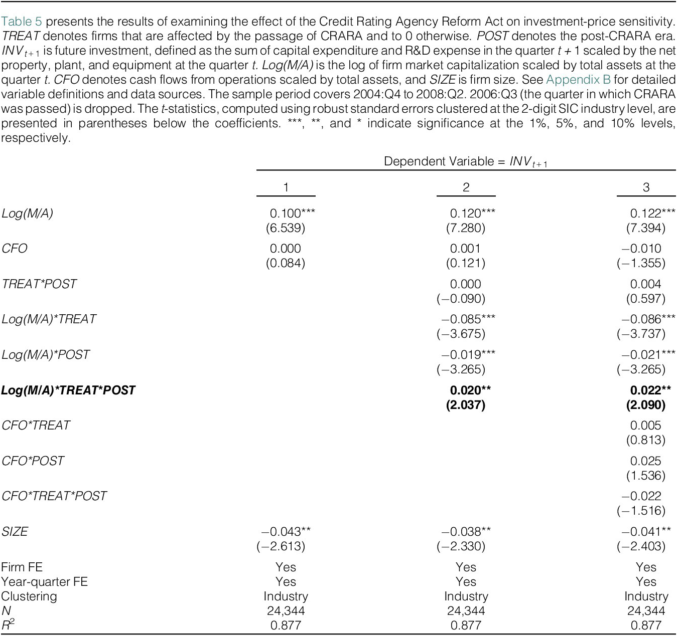
We present the results of estimating equation (2) in Table 5. Model 1 presents the baseline result without treatment, where INV t + 1 is regressed on Log(M/A), our price-based measure of investment opportunities. We also include CFO and SIZE. We standardize Log(M/A) and CFO by subtracting the sample mean and scaling by the standard deviation to infer the coefficient as the marginal effect of one standard deviation. The coefficient on Log(M/A) is 0.100 (p-value < 0.01), demonstrating that future investment increases by 10.0% in response to a one standard deviation increase in a price-based measure of investment opportunities.

TABLE 5 Long description
The table presents regression results for the dependent variable I N V sub t plus 1 across three numbered columns.
Key variables and coefficients (with t-statistics in parentheses):
- Log(M/A): 0.100 (6.539) in column 1; 0.120 (7.280) in column 2; 0.122 (7.394) in column 3. All are significant at the 1 percent level.
- C F O: 0.000 (0.084) in column 1; 0.001 (0.121) in column 2; -0.010 (-1.355) in column 3.
- T R E A T * P O S T: 0.000 (-0.090) in column 2; 0.004 (0.597) in column 3.
- Log(M/A) * T R E A T: -0.085 (-3.675) in column 2; -0.086 (-3.737) in column 3. Both significant at the 1 percent level.
- Log(M/A) * P O S T: -0.019 (-3.265) in column 2; -0.021 (-3.265) in column 3. Both significant at the 1 percent level.
- Log(M/A) * T R E A T * P O S T: 0.020 (2.037) in column 2; 0.022 (2.090) in column 3. Both significant at the 5 percent level.
- C F O * T R E A T: 0.005 (0.813) in column 3.
- C F O * P O S T: 0.025 (1.536) in column 3.
- C F O * T R E A T * P O S T: -0.022 (-1.516) in column 3.
- S I Z E: -0.043 (-2.613) in column 1; -0.038 (-2.330) in column 2; -0.041 (-2.403) in column 3. All significant at the 5 percent level.
Model Specifications:
- Firm F E: Yes for all columns.
- Year-quarter F E: Yes for all columns.
- Clustering: Industry for all columns.
- N: 24,344 for all columns.
- R-squared: 0.877 for all columns.
Model 2 shows the impact of CRARA on investment-price sensitivity. The coefficient on Log(M/A)*TREAT*POST is positive, 0.020, and significant (p-value < 0.05), indicating an increase in investment-price sensitivity after CRARA. We interpret these results as initial evidence that managers increasingly rely on stock prices to guide their investment decisions because stock prices contain more private information they wish to learn after the passage of CRARA. In model 3, we include a nonprice-based measure for investment opportunities (variables interacted with CFO) and find an insignificant coefficient on CFO*TREAT*POST. Not only does this result support the price-based learning channel, but it also mitigates the confounding effect of time-varying investment opportunities.
In combination with the results in Table 4, the results in Table 5 suggest that CRARA incentivizes informed traders to gather and trade on information, some of which is new to managers, and hence managers rely more on stock prices after the passage of CRARA.
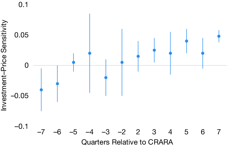
Figure 2 shows the results of assessing the parallel trends assumption. We plot the coefficients that are obtained from estimating regressions similar to model 3 of Table 5 by interacting 12 indicator variables equal to 1 for each quarter surrounding CRARA with Log (M/A) in place of POST. Differences in investment-price sensitivity appear to have increased 2 quarters after the passage of CRARA, suggesting that it took a few quarters until managers’ investment decisions responded to the newly available private information in prices, presumably due to adjustment costs. This finding comports with those of Jayaraman and Wu (Reference Jayaraman and Wu2019). However, treatment and control groups seem to show some modest differences in a few quarters prior to the passage of CRARA. In general, we interpret the results from Figure 2 as not indicating a violation of parallel trends in the pretreatment period. Nonetheless, we admit that there is some concern about time-varying correlated omitted variables. We mitigate this concern by running a battery of cross-sectional and falsification tests and examining future performance in the subsequent sections.
Figure 2 shows difference-in-differences coefficients on investment-price sensitivity for each event-time. We define QTR(−7) as an indicator variable equal to 1 for observations in the 7 quarters before CRARA and 0 otherwise. The remaining indicators are defined analogously. QTR(−1) and QTR(+1) are omitted, serving as the benchmark. The dots (lines) represent coefficient estimates (95% confidence intervals).

FIGURE 2 Long description
A line graph with a horizontal zero baseline. The vertical Y-axis is labeled Investment-Price Sensitivity with a scale from negative 0.1 to 0.1 in increments of 0.05. The horizontal X-axis is labeled Quarters Relative to C R A R A with twelve discrete time points. From left to right, the data points are as follows.
* Negative 7: Coefficient near negative 0.04 with a wide confidence interval.
* Negative 6: Coefficient near negative 0.03.
* Negative 5: Coefficient slightly above 0.
* Negative 4: Coefficient near 0.02 with the largest vertical confidence interval.
* Negative 3: Coefficient near negative 0.02.
* Negative 2: Coefficient near 0.
* 2: Coefficient near 0.015.
* 3: Coefficient near 0.025.
* 4: Coefficient near 0.02.
* 5: Coefficient near 0.04.
* 6: Coefficient near 0.02.
* 7: Coefficient near 0.05 with the narrowest confidence interval.
Overall, the coefficients show a general upward trend from negative values before the event to consistently positive values in the later quarters following the omitted benchmark period.
D. Cross-Sectional Tests: Types of Information Driving the Effects of CRARA on Investment-Price Sensitivity
In this section, we explore whether the treatment effect varies with firm characteristics that correlate with types of information more conducive to managerial learning.
1. Uncertainties Where Investors Have an Informational Advantage
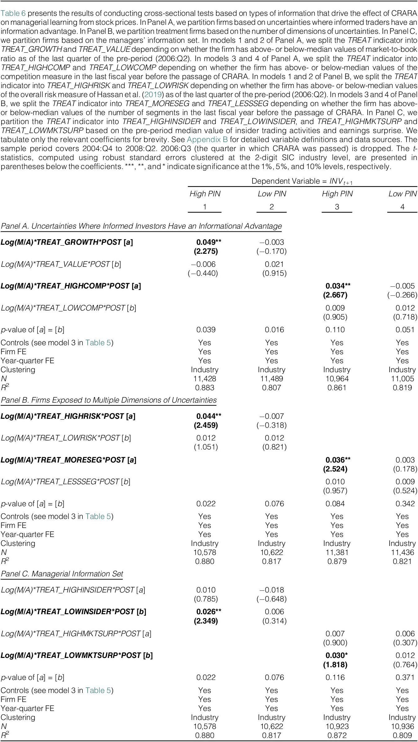
A salient feature of learning models is that investors’ information advantage lies in assessing certain types of uncertainties, such as growth opportunities, industry competition, or factors that require market-wide analysis, such as policy uncertainty (Bai et al. (Reference Bai, Philippon and Savov2016), Goldstein and Yang (Reference Goldstein and Yang2019), and Goldstein et al. (Reference Goldstein, Yang and Zuo2023)). We thus predict that the passage of CRARA facilitates managerial learning more among firms about which investors tend to have an information advantage relative to managers. Studies posit that growth opportunities and product market competition are the types of uncertainties where investors’ informational advantage lies (Jayaraman and Wu (Reference Jayaraman and Wu2019), Goldstein et al. (Reference Goldstein, Yang and Zuo2023)). We follow Goldstein et al. (Reference Goldstein, Yang and Zuo2023) and use firms’ market-to-book ratio as a proxy for growth opportunities. We split the TREAT indicator into two indicators representing treatment firms with above-median (TREAT_GROWTH) and below-median (TREAT_VALUE) values of firms’ growth opportunities. Then, we modify equation (2) by interacting these indicators with POST and Log(M/A) to examine the varied treatment effect between growth and value firms.
Since competition is complex, we rely on both industry and firm measures. Specifically, we use industry concentration (HHI) and a measure of product similarity provided by Hoberg and Phillips (Reference Hoberg and Phillips2016). We then take the average of the ranks of the inverse of HHI and product similarity to construct a composite measure of competition. We partition treatment firms with above-median (TREAT_HIGHCOMP) and below-median (TREAT_LOWCOMP) values of this competition measure. We interact these indicators with POST and Log(M/A) to examine the heterogeneous treatment effect between firms with high and low competition.
To better identify the effect of CRARA, we estimate this specification and remaining cross-sectional tests separately for treatment firms with high versus low informed trading (i.e., high and low PIN treatment firms) because studies show that managerial learning from prices is more pronounced when informed trading is high (e.g., Chen et al. (Reference Chen, Goldstein and Jiang2007)).
We present our results in Panel A of Table 6. Consistent with our expectations, in models 1 and 2, the coefficient on Log(M/A)*TREAT_GROWTH*POST of the high PIN group is positive (0.049) and significant at the 5% level, whereas the corresponding coefficient of value firms, Log(M/A)*TREAT_VALUE*POST, is insignificant. The two coefficients differ at p-value = 0.039. In models 3 and 4, we present our results of the differential treatment effect with respect to the level of competition. The coefficient on Log(M/A)*TREAT_HIGHCOMP*POST of the high PIN group is positive, 0.034, and significant at the 5% level, whereas the coefficient on Log(M/A)* TREAT_LOWCOMP*POST is insignificant. However, the difference between the two subsamples is insignificant at the conventional level (p-value = 0.110).

TABLE 6 Long description
The table displays regression results for the dependent variable I N V sub t+1 across four columns. Columns 1 and 3 represent High P I N (Probability of Informed Trading), while columns 2 and 4 represent Low P I N.
Panel A, Uncertainties Where Informed Investors Have an Informational Advantage:
* Log(M/A)*TREAT_GROWTH*POST [a]: Column 1 (High P I N) shows a significant coefficient of 0.049 (t-stat 2.275). Column 2 (Low P I N) is -0.003.
* Log(M/A)*TREAT_HIGHCOMP*POST [a]: Column 3 (High P I N) shows a significant coefficient of 0.034 (t-stat 2.667). Column 4 (Low P I N) is -0.005.
* p-values for [a] = [b] range from 0.016 to 0.110.
Panel B, Firms Exposed to Multiple Dimensions of Uncertainties:
* Log(M/A)*TREAT_HIGHRISK*POST [a]: Column 1 (High P I N) shows 0.044 (t-stat 2.459). Column 2 (Low P I N) is -0.007.
* Log(M/A)*TREAT_MORESEG*POST [a]: Column 3 (High P I N) shows 0.036 (t-stat 2.524). Column 4 (Low P I N) is 0.003.
Panel C, Managerial Information Set:
* Log(M/A)*TREAT_LOWINSIDER*POST [b]: Column 1 (High P I N) shows 0.026 (t-stat 2.349).
* Log(M/A)*TREAT_LOWMKTSURP*POST [b]: Column 3 (High P I N) shows 0.030 (t-stat 1.818).
All models include Controls, Firm F E, and Year-quarter F E, with clustering by Industry. R-squared values range from 0.807 to 0.883, and N ranges from 10,578 to 11,489.
2. Firms Exposed to Multiple Dimensions of Uncertainties
Learning models assume that firms face multiple kinds of uncertainties, about which informed traders acquire private information to try to profit from trading on the acquired information (Goldstein and Yang (Reference Goldstein and Yang2015), (2019)). This assumption suggests that the effect of CRARA on investment-price sensitivity strengthens among firms with more uncertainties. We test this prediction by employing two proxies. First, we use the overall risk that each firm faces. To measure overall risk, we exploit the measure developed by Hassan, Hollander, van Lent, and Tahoun (Reference Hassan, Hollander, van Lent and Tahoun2019), which counts the number of risk-related words from the firm’s earnings conference call scripts. Second, we use the number of segments (both business and geographic). This proxy dovetails nicely with the conceptual framework of learning models.Footnote 7
As in the above heterogeneity tests, we split the TREAT indicator into two indicators representing treatment firms with above-median (TREAT_HIGHRISK) and below-median (TREAT_LOWRISK) values of the overall risk measure. Likewise, we split the TREAT indicator into two indicators denoting treatment firms with above-median (TREAT_MORESEG) and below-median (TREAT_LESSSEG) values of the total number of segments. Then, we modify equation (2) by interacting these indicators with POST and Log(M/A).
We present the results in Panel B of Table 6. The results are consistent with our predictions. Models 1 and 2 present the differential treatment effect between firms with high and low risk. Focusing on model 1 of the high PIN group shows that the coefficient for high-risk firms (Log(M/A)*TREAT_HIGHRISK*POST) is positive (0.044) and significant at the 5% level, whereas the corresponding coefficient for low-risk firms (Log(M/A)*TREAT_LOWRISK*POST) is insignificant. The two coefficients statistically differ from each other at p-value = 0.022. Models 3 and 4 present the heterogeneous treatment effect with respect to the number of segments. The coefficient on Log(M/A)*TREAT_MORESEG*POST of the high PIN group is positive and significant at the 5% level, whereas that on Log(M/A)*TREAT_LESSSEG*POST is insignificant. The differences in coefficients between the two groups are significant (p-value = 0.084).
3. Managers’ Own Information
The previous cross-sectional tests exploit firm characteristics associated with types of information in prices that can help managers make investment decisions. However, managers factor into their investment decisions all available information, including their own information, as well as information in stock prices incorporated by informed traders via trading (e.g., Bai et al. (Reference Bai, Philippon and Savov2016)). Studies show that managers’ own information moderates their reliance on market feedback (Chen et al. (Reference Chen, Goldstein and Jiang2007), Bai et al. (Reference Bai, Philippon and Savov2016), and Jayaraman and Wu (Reference Jayaraman and Wu2020)). This suggests that the increase in investment-price sensitivity associated with CRARA will be muted when managers are privately better informed about the sources of uncertainty affecting firm value.
To test this prediction, we follow (e.g., Chen et al. (Reference Chen, Goldstein and Jiang2007)) and use the number of shares bought and sold by CEOs and CFOs (INSIDER) and earnings surprises (MKTSURP), measured as the absolute abnormal returns around earnings announcements, as proxies for managers’ private information. The idea is as follows: Managers with more private information trade more, and their greater trading indicates their greater information; managers, for example, know earnings before the announcement, and thus, higher (absolute) stock reactions to announcements indicate more managerial information.
We split the TREAT indicator into two indicators denoting treatment firms with above-median (TREAT_HIGHINSIDER or TREAT_HIGHMKTSURP) and below-median (TREAT_LOWINSIDER or TREAT_LOWMKTSURP) values of insider trading and earnings surprises. Then, we modify equation (2) by interacting these indicators with POST and Log(M/A) to examine the heterogenous treatment effect between firms with high and low managerial information.
We present the results in Panel C of Table 6. The results support our prediction. The coefficient on Log(M/A)*TREAT_LOWINSIDER*POST of the high PIN group (model 1) is positive and significant at the 5% level, whereas that for firms with high insider trading (Log(M/A)*TREAT_HIGHINSIDER*POST) is insignificant. The two coefficients differ at p-value = 0.022. We also observe similar patterns in models 3 and 4, with only the coefficient on Log(M/A)*TREAT_LOWMKTSURP*POST being significant for the high PIN group. These results indicate that managers’ private information moderates the effects of CRARA on managers’ reliance on price signals. All the cross-sectional findings substantiate our inferences that the increase in investment-price sensitivity associated with the passage of CRARA is due to price-based learning and helps mitigate the concern of time-varying omitted variable bias.
We, however, hasten to add a caveat that these findings provide suggestive rather than conclusive evidence. Differences across subsamples are not consistently significant, and when they are, they are typically concentrated among treatment firms with high levels of informed trading. Moreover, some of the significant differences vanish once we use the matched control sample, the results that we present in Table OA4 in the Supplementary Material.
E. Evidence on a Specific Type of Uncertainty: Accounting Fraud Risk
The results thus far are consistent with CRARA lowering informed traders’ uncertainty about firm creditworthiness, acquiring more information that is new to managers, and thus leading to more managerial learning from stock prices. To substantiate this inference, we examine accounting fraud risk as one source of firm-specific creditworthiness.
CRAs’ failure to downgrade the credit ratings of firms that were subsequently shown to have committed accounting fraud (e.g., Enron and WorldCom) damaged their reputation as a credible and reliable source of information about creditworthiness. In response, investors are likely to spend more time and effort assessing accounting fraud risk on their own and less collecting information about other aspects of firm value. Consequently, CRARA may restore the credibility of credit ratings as a source of information about firms’ accounting fraud risk. This argument is consistent with an increase in reporting credibility in Table 2. Following the passage of CRARA, investors acquire less information about firms’ fraud risk and more information about factors that may be new to firm managers. This substitution effect is expected to strengthen among firms whose earnings quality was worse before CRARA.
To capture earnings quality, we follow prior studies (e.g., Ahmed, Li, and Xu (Reference Ahmed, Li and Xu2020)) and use multiple proxies. First, we use modified Jones discretionary accruals, measured as the absolute value of residuals from the Dechow, Sloan, and Sweeney (Reference Dechow, Sloan and Sweeney1995) model augmented by including nonlinear performance and growth controls (Kothari, Leone, and Wasley (Reference Kothari, Leone and Wasley2005), Collins, Pungaliya, and Vijh (Reference Collins, Pungaliya and Vijh2017)). Second, we use Dechow–Dichev discretionary accruals, measured as the absolute value of residuals from the Dechow and Dichev (Reference Dechow and Dichev2002) model modified by McNichols (Reference McNichols2002) with nonlinear performance and growth controls. Thus, lower values of these accrual measures indicate higher EQ. We provide detailed measurements of these variables in Appendix B.
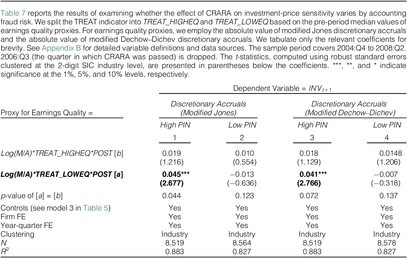
To test our prediction, we split the TREAT indicator into two indicators representing treatment firms with below-median (TREAT_HIGHEQ) and above-median (TREAT_LOWEQ) values of the two accrual measures, respectively. Then, we modify equation (2) by interacting these indicators with POST and Log(M/A) to assess the differential treatment effect on investment-price sensitivity between high versus low EQ firms.
Table 7 presents the results. The results support our prediction that the treatment effect strengthens for firms with pre-CRARA poor earnings quality, especially when there is active informed trading. The coefficients on Log(M/A)*TREAT_LOWEQ*POST of the high PIN group (models 1 and 3) are 0.045 and 0.041 and significant at the 1% level, whereas the corresponding coefficients for high EQ firms are insignificant. The differences in the two coefficients between high and low EQ subgroups are statistically significant at the 5% level for model 1 and at the 10% level for model 3. In sum, these results suggest that CRARA assuages investors’ concerns about firms’ accounting fraud risk, leading to an increase in investment-price sensitivity.

TABLE 7 Long description
The table presents regression results for the dependent variable I N V sub t plus 1. It is divided into two main sections based on the Proxy for Earnings Quality: Discretionary Accruals (Modified Jones) for columns 1 and 2, and Discretionary Accruals (Modified Dechow-Dichev) for columns 3 and 4. Each proxy is further split into High P I N and Low P I N subgroups.
Key data points include:
* Log(M/A) times T R E A T underscore H I G H E Q times P O S T [b]: Coefficients are 0.019 (column 1), 0.010 (column 2), 0.018 (column 3), and 0.0148 (column 4).
* Log(M/A) times T R E A T underscore L O W E Q times P O S T [a]: Coefficients are 0.045 (column 1, significant at 1 percent level), -0.013 (column 2), 0.041 (column 3, significant at 1 percent level), and -0.007 (column 4).
* p-value of [a] = [b]: Values are 0.044, 0.123, 0.072, and 0.137 respectively.
All models include Controls, Firm F E, and Year-quarter F E, with clustering by Industry. Sample sizes (N) range from 8,519 to 8,578, and R-squared values range from 0.827 to 0.883.
F. Future Performance
We interpret an increase in investment-price sensitivity following the passage of the act as consistent with managers learning from investor information, indicating an improvement in real efficiency. However, some concerns still exist. First, an increase in investment-price sensitivity post-CRARA may simply reflect changes in information available to investors. In that case, the increase would result from greater alignment between managers’ and investors’ information, even if managers have not altered their investment policies based on investors’ information. Second, an increase in investment-price sensitivity may be consistent with managers increasing investment to cater to overly optimistic investors in the post-CRARA period (Polk and Sapienza (Reference Polk and Sapienza2008)). To assuage these concerns, we test for an improvement in firms’ future performance. If price-based learning entails richer information in stock prices that is new to managers after CRARA’s passage, we expect an increase in firms’ future performance as managers rely more on stock prices.
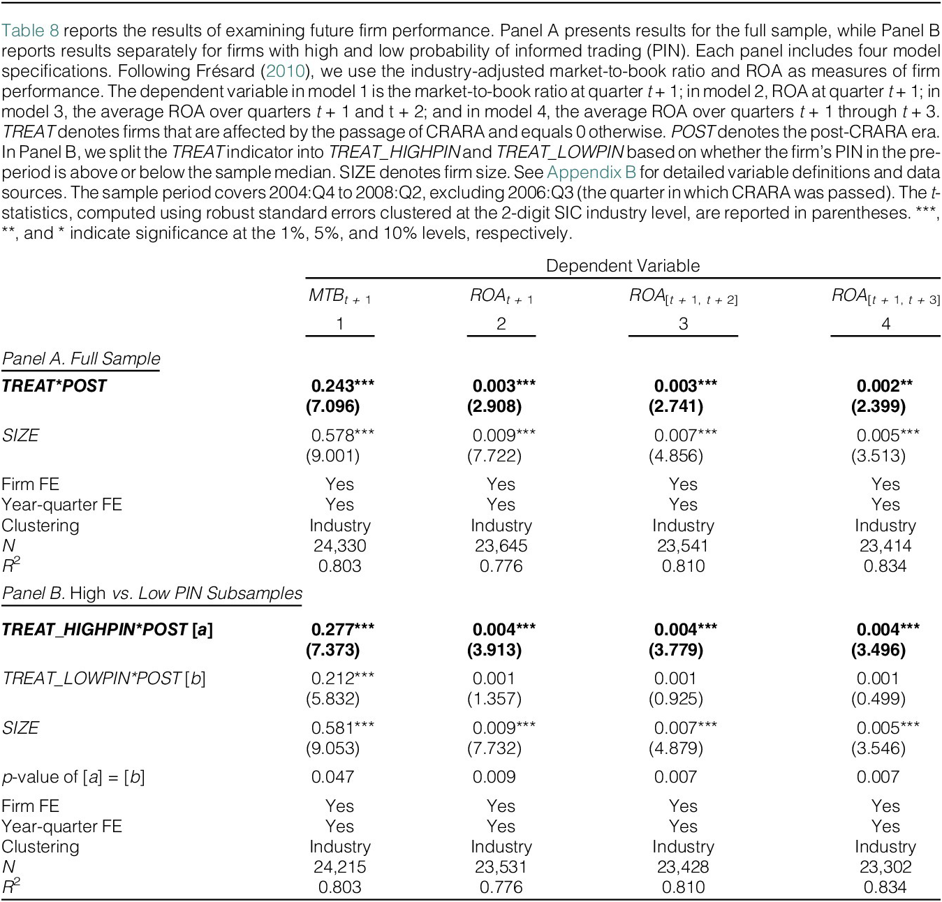
Table 8 presents the results. We follow Frésard (Reference Frésard2010) and measure future performance with industry-adjusted market-to-book (MTB) and return on assets (ROA). We measure ROA over various horizons—one-quarter-ahead ROA (ROA [t + 1]) and average ROA over the next 2 and 3 quarters (ROA [t + 1, t + 2] and ROA [t + 1, t + 3])—and regress these measures on TREAT*POST and SIZE. Using these measures, we find evidence of improvement in firm performance. In model 1, we find a significant coefficient on TREAT*POST, suggesting that treatment firms experience a significant increase in market-to-book following the passage of the act. In models 2–4, we also find significant coefficients on TREAT*POST, indicating that the treatment firms significantly improve accounting performance after CRARA.

TABLE 8 Long description
The table is divided into two panels. The header identifies four columns of dependent variables: 1 M T B sub t plus 1, 2 R O A sub t plus 1, 3 R O A sub t plus 1, t plus 2, and 4 R O A sub t plus 1, t plus 3.
Panel A. Full Sample:
- T R E A T asterisk P O S T: Coefficients are 0.243, 0.003, 0.003, and 0.002, with t-statistics in parentheses ranging from 2.399 to 7.096. All are statistically significant.
- S I Z E: Coefficients are 0.578, 0.009, 0.007, and 0.005, all significant at the 1 percent level.
- Fixed Effects: Firm F E and Year-quarter F E are included (Yes) for all models.
- Clustering: Industry for all models.
- N: Observations range from 24,330 in model 1 to 23,414 in model 4.
- R-squared: Values range from 0.776 to 0.834.
Panel B. High vs. Low P I N Subsamples:
- T R E A T underscore H I G H P I N asterisk P O S T [a]: Coefficients are 0.277, 0.004, 0.004, and 0.004, all significant at the 1 percent level.
- T R E A T underscore L O W P I N asterisk P O S T [b]: Coefficients are 0.212 (significant), 0.001, 0.001, and 0.001 (not significant).
- S I Z E: Coefficients are 0.581, 0.009, 0.007, and 0.005.
- p-value of [a] = [b]: Values are 0.047, 0.009, 0.007, and 0.007.
- N: Observations range from 24,215 to 23,302.
- R-squared: Values are identical to Panel A.
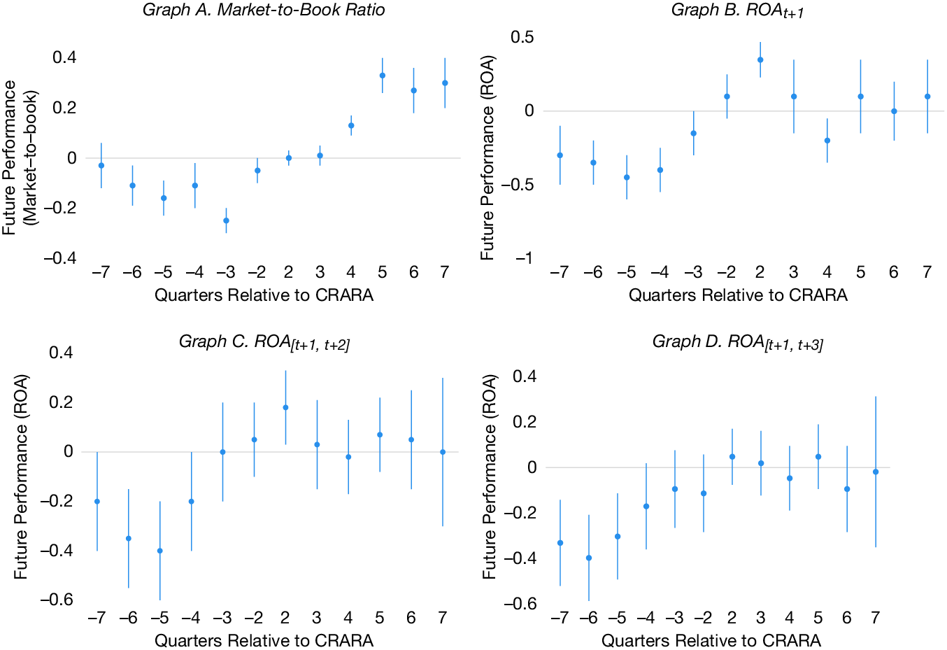
Figure 3 shows the results of assessing the parallel trends assumption. We plot the coefficients that are obtained from estimating regressions by interacting with 12 indicator variables equal to 1 for each quarter surrounding CRARA in place of POST with TREAT. Visual inspection suggests that the effect on market-to-book seems to emerge with some delay, whereas the effect on accounting performance appears to rise more rapidly, and that these effects appear to be somewhat sustained in the post-CRARA period.
Figure 3 shows difference-in-differences coefficients on future performance for each event-time. As measures of future performance, Graphs A–D use the market-to-book ratio at t + 1, ROA at t + 1, average ROA over t + 1 and t + 2, and average ROA over t + 1 to t + 3. We define QTR(−7) as an indicator variable equal to 1 for observations in the 7 quarters before CRARA and 0 otherwise. The remaining indicators are defined analogously. QTR(−1) and QTR(+1) are omitted, serving as the benchmark. The dots (lines) represent coefficient estimates (95% confidence intervals).

FIGURE 3 Long description
A four-panel set of coefficient plots. Each graph shares a common x-axis labeled Quarters Relative to C R A R A, with discrete points at negative 7 through negative 2 and positive 2 through positive 7. The y-axis represents Future Performance.
* Graph A Market-to-Book Ratio. The y-axis ranges from negative 0.4 to 0.4. Coefficients are slightly negative before the event, reaching a trough at quarter negative 3, then show a sharp upward trend starting at quarter 4, peaking around 0.3 in quarters 5 through 7.
* Graph B R O A sub t plus 1. The y-axis ranges from negative 1 to 0.5. Data points fluctuate between negative 0.5 and 0.0 before the event, spike to a peak above 0.3 at quarter 2, and then stabilize near 0.0 for quarters 4 through 7.
* Graph C R O A sub open bracket t plus 1 comma t plus 2 close bracket. The y-axis ranges from negative 0.6 to 0.4. Coefficients are negative between quarters negative 7 and negative 4, then rise toward the zero line. Post-event data points remain near zero with wider 95 percent confidence intervals.
* Graph D R O A sub open bracket t plus 1 comma t plus 3 close bracket. The y-axis ranges from negative 0.6 to 0.4. Similar to Graph C, values are negative in the pre-event period, specifically between negative 7 and negative 5, then trend upward to fluctuate around the zero benchmark from quarter 2 onward.
In Panel B, we split treatment firms into high and low PIN subsamples because managers’ reliance on stock prices as a source of information to guide investment decisions strengthens for firms with more informed trading (Chen et al. (Reference Chen, Goldstein and Jiang2007)). The results support our prediction. The coefficients on TREAT_HIGHPIN*POST are positive and significant at the 1% level, whereas the coefficients on TREAT_LOWPIN*POST are insignificant. The two coefficients differ significantly (p-value < 0.05 or better). Overall, the results support the argument that the credibility of mandatory disclosure by CRAs improves real efficiency via managerial learning from stock prices.Footnote 8
G. Alternative Explanations
1. Corporate Governance
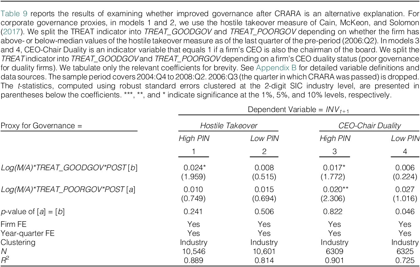
A compelling alternative explanation is that investment-price sensitivity increases among firms affected by CRARA due to increased monitoring. If CRAs better monitor firms following CRARA, managers may pursue fewer self-dealing investments, such as empire-building, resulting in an increase in investment-price sensitivity. To assess this explanation, we conduct falsification tests by exploring whether the increase in investment-price sensitivity associated with CRARA varies with the strength of corporate governance.
We measure the strength of firms’ corporate governance with two proxies: i) Cain, McKeon, and Solomon’s (Reference Cain, McKeon and Solomon2017) H-index capturing hostile takeover threats and ii) CEO-chair duality. As in our cross-sectional tests, we split the TREAT indicator into two indicators, denoting treatment firms with good governance (TREAT_GOODGOV) and those with poor governance (TREAT_POORGOV). Firms with above-median values of the H-index are categorized as well-governed firms, while firms with below-median values are categorized as poorly governed. Firms where CEOs are also the chairperson of the board are characterized as poorly governed, while other firms are characterized as well governed. We present the results in Table 9. Across the two measures of governance, we do not find evidence supporting improved monitoring as an alternative explanation.

TABLE 9 Long description
The table is organized into four columns. The dependent variable for all columns is I N V sub t plus 1. Columns 1 and 2 use Hostile Takeover as the Proxy for Governance, while Columns 3 and 4 use C E O-Chair Duality. Columns 1 and 3 represent High P I N, and Columns 2 and 4 represent Low P I N.
Key data rows include:
* Log M forward slash A times T R E A T underscore G O O D G O V times P O S T [b]: Column 1 is 0.024* with a t-stat of 1.959. Column 2 is 0.008 with a t-stat of 0.515. Column 3 is 0.017* with a t-stat of 1.772. Column 4 is 0.006 with a t-stat of 0.224.
* Log M forward slash A times T R E A T underscore P O O R G O V times P O S T [a]: Column 1 is 0.010 with a t-stat of 0.749. Column 2 is 0.015 with a t-stat of 0.694. Column 3 is 0.020** with a t-stat of 2.306. Column 4 is 0.027 with a t-stat of 1.016.
* p-value of [a] = [b]: Column 1 is 0.241, Column 2 is 0.506, Column 3 is 0.822, and Column 4 is 0.046.
All columns include Firm F E and Year-quarter F E, with clustering by Industry.
Statistical summary:
* N: Column 1 is 10,546; Column 2 is 10,601; Column 3 is 6,309; Column 4 is 6,325.
* R-squared: Column 1 is 0.889; Column 2 is 0.814; Column 3 is 0.901; Column 4 is 0.725.
2. Other Alternative Explanations
We also assess other alternative explanations. First, we evaluate the possibility that CRA disclosure directly benefits managers by providing new information after CRARA. If so, better future performance among treatment firms could be driven by managers learning new information from CRAs, not from stock prices. Second, we assess the Great Recession as an alternative explanation. If the recession significantly limited firms’ ability to access capital markets, especially for firms with no credit ratings (Duchin, Ozbas, and Sensoy (Reference Duchin, Ozbas and Sensoy2010)), investment-price sensitivity would increase for firms with credit ratings relative to those without. Third, we examine managers’ disclosure changes as an alternative explanation. If CRARA results in a decrease in management earnings forecasts (Sethuraman (Reference Sethuraman2019)), reductions in these disclosures will encourage informed traders’ private information production (Chen, Ng, and Yang (Reference Chen, Ng and Yang2021)), resulting in more reliance on stock prices in the post-CRARA period. In the results presented in Tables OA1–OA3 in the Supplementary Material, we conclude that these are unlikely explanations.
H. Robustness Tests
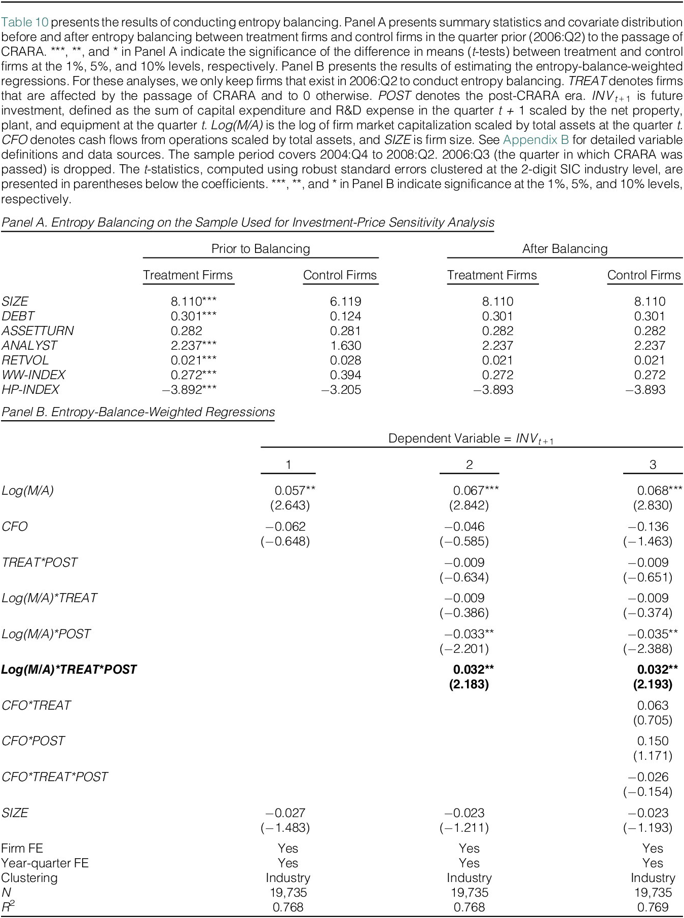
To mitigate the concern of pre-CRARA differences between treatment and control groups, we entropy balance treatment and control firms on a set of covariates based on the factors that Standard & Poor’s considers when it rates the firms (S&P Global Ratings (2017), (2022)): firm size (SIZE), leverage (DEBT), asset turnover (ASSETTURN), the number of analysts following (ANALYST), and uncertainty (RETVOL). We augment these covariates with two proxies for financial constraints, the WW index of Whited and Wu (Reference Whited and Wu2006) (WW-INDEX) and the HP index of Hadlock and Pierce (Reference Hadlock and Pierce2010) (HP-INDEX), because treatment and control firms likely face different levels of financial constraints. We reweight control firms based on these seven variables in the year prior to the enactment of CRARA to ensure covariate balance across treatment and control samples (Hainmueller (Reference Hainmueller2012), McMullin and Schonberger (Reference McMullin and Schonberger2020)). We present the covariate balance between treatment and control firms in Panel A of Table 10. By construction, both samples exhibit no differences across the seven covariates after entropy balancing. We then estimate the entropy-balance-weighted regressions and present the results in Panel B of Table 10. Our results are robust to this alternative research design.Footnote 9

TABLE 10 Long description
Panel A, titled Entropy Balancing on the Sample Used for Investment-Price Sensitivity Analysis, compares Treatment and Control firms Prior to Balancing and After Balancing across seven variables. Prior to balancing, significant differences exist in S I Z E (8.110 vs 6.119), D E B T (0.301 vs 0.124), A N A L Y S T (2.237 vs 1.630), R E T V O L (0.021 vs 0.028), W W-I N D E X (0.272 vs 0.394), and H P-I N D E X (-3.892 vs -3.205). After balancing, all variables for Control firms are adjusted to match the Treatment firms exactly (e.g., S I Z E is 8.110 for both).
Panel B, titled Entropy-Balance-Weighted Regressions, presents three regression models where the dependent variable is I N V sub t+1.
* Model 1 includes L o g (M / A), C F O, and S I Z E, with a L o g (M / A) coefficient of 0.057.
* Model 2 adds interaction terms, showing a significant triple interaction for L o g (M / A) * T R E A T * P O S T of 0.032 (t-stat 2.183).
* Model 3 adds further interactions with C F O, maintaining the significant L o g (M / A) * T R E A T * P O S T coefficient at 0.032 (t-stat 2.193).
All models include Firm F E, Year-quarter F E, and Industry clustering, with N = 19,735 and R-squared values around 0.768.
Next, we address measurement errors present in market-based proxies for investment opportunities (Erickson and Whited (Reference Erickson and Whited2000), (Reference Erickson and Whited2006), (Reference Erickson and Whited2012)) by using a method of Erickson et al. (Reference Erickson, Jiang and Whited2014). This method leverages higher-order cumulants derived from the distribution of market-to-book, aiming to address the impact of fluctuations in market values overlooked by managers. We also show the robustness of our results to alternative definitions of market-based investment opportunities. For our analyses, we follow Bai et al. (Reference Bai, Philippon and Savov2016) and use the log of the market value of equity to total assets (Log(M/A)). We assess whether our results are sensitive to the unlogged M/A and the traditional Tobin’s Q. In Table 11, we find our results are robust to the correction of measurement error in investment opportunities and alternative definitions of investment opportunities. We also assess the robustness of the results from cross-sectional tests and find that the significant differences we report in Table 5 remain, with an exception for high versus low levels of insider trading. See Table OA6 of the Supplementary Material.

TABLE 11 Long description
The table presents regression results where the dependent variable is I N V sub t plus 1. It consists of two columns of results.
* M forward slash A: Column 1 shows 0.310 with a t-statistic of 93.79. Column 2 is blank.
* Q: Column 1 is blank. Column 2 shows 0.300 with a t-statistic of 98.96.
* C F O: Column 1 shows minus 0.289 -8.001. Column 2 shows minus 0.282 -7.821.
* T R E A T asterisk P O S T: Column 1 shows minus 0.122 -6.250. Column 2 shows minus 0.142 -7.253.
* M forward slash A asterisk T R E A T: Column 1 shows minus 0.139 -22.24. Column 2 is blank.
* M forward slash A asterisk P O S T: Column 1 shows minus 0.004 -0.522. Column 2 is blank.
* M forward slash A asterisk T R E A T asterisk P O S T: Column 1 shows 0.017 1.980. Column 2 is blank.
* Q asterisk T R E A T: Column 1 is blank. Column 2 shows minus 0.143 -25.08.
* Q asterisk P O S T: Column 1 is blank. Column 2 shows 0.002 0.381.
* Q asterisk T R E A T asterisk P O S T: Column 1 is blank. Column 2 shows 0.016 2.111.
* C F O asterisk T R E A T: Column 1 shows 1.698 3.838. Column 2 shows 1.387 3.119.
* C F O asterisk P O S T: Column 1 shows minus 0.558 -0.920. Column 2 shows minus 0.611 -1.006.
* C F O asterisk T R E A T asterisk P O S T: Column 1 shows 2.831 3.739. Column 2 shows 3.188 4.185.
* S I Z E: Column 1 shows minus 0.085 -13.68. Column 2 shows minus 0.085 -13.62.
* Firm F E: Yes for both columns.
* Year-quarter F E: Yes for both columns.
* Clustering: Industry for both columns.
* N: 24,195 for column 1 and 24,129 for column 2.
* Pseudo R super 2: 0.173 for column 1 and 0.167 for column 2.
V. Conclusion
This article examines the effects of the credibility of mandatory disclosure by CRAs on stock price informativeness and managerial learning from stock prices. Using CRARA in 2006 as a setting, we find increases in stock price informativeness and investment-price sensitivity for affected firms compared to control firms. Cross-sectional analyses show the increase in investment-price sensitivity strengthens for growth firms, firms confronting more competition, firms with multiple uncertainties, firms with poorer managerial information, and firms with poor earnings quality. Further, affected firms experience an improvement in future performance compared to control firms. These findings contribute to the managerial learning literature by examining the credibility of mandatory disclosures from an information intermediary, rather than focusing on mandatory disclosures by firms.
We add several caveats and avenues for future research. First, our study is subject to the inherent challenge that information in stock prices, not to mention information type, is unobservable. As such, our findings are subject to the possibility that correlated omitted factors are responsible for our results. Nonetheless, the detailed assessment of alternative explanations and the results of improved future performance support price-based learning. Relatedly, readers should exercise caution in drawing causal inferences because having an S&P credit rating is endogenous and the market feedback effect of mandatory disclosures, either by firms or information intermediaries, is context specific. Thus, we believe that our results should be interpreted in the context of CRARA, and a different conclusion may arise in other settings because, as highlighted by Goldstein and Yang (Reference Goldstein and Yang2019), whether disclosures improve or impede managerial learning depends upon the type of information being disclosed by a given intermediary. We leave this for future research. Another interesting question for future research is how disclosures by CRAs affect managerial learning from bond prices.
Appendix A. Details on the Provisions of the Credit Rating Agency Reform Act of 2006
This appendix provides details of the provisions from the Senate Report 109-326 and Public Law 109-291 regarding Credit Rating Agency Reform Act of 2006.

Long description
The table is organized into four main rows.
Row 1: Enacted. The date is September 29, 2006.
Row 2: Purpose of the legislation. To improve ratings quality for investor protection and public interest by fostering accountability, transparency, and competition in the credit rating agency industry.
Row 3: Overview of the regulatory landscape. It notes that the largest N R S R O s, S and P and Moody’s, have significant power but were previously virtually unregulated. Following scandals like Enron and WorldCom, this act addresses the lack of oversight, conflicts of interest, and anticompetitive practices in rating agencies.
Row 4: Details of the provisions of C R A R A. This section lists eight bulleted requirements for agencies registering as N R S R O s:
• Disclose ratings performance and conflicts of interest.
• Provide procedures and methodologies for determining ratings.
• Implement policies to prevent misuse of nonpublic information.
• Provide the organizational structure of the agency.
• Disclose the presence or absence of a code of ethics.
• Disclose any conflict of interest related to rating issuance.
• Provide a confidential list of the 20 largest issuers and subscribers by net revenue.
• Provide any other information deemed necessary by the Commission for public interest or investor protection.
Appendix B. Variable Definitions and Data Sources
Outcome Variables
- CAR_3DAY:
-
Cumulative abnormal return in the 3-day period centering on quarterly earnings announcement dates (−1, 0, 1). Abnormal return is measured as the natural logarithm of 1 plus actual return of firm i on day d minus the natural logarithm of 1 plus expected return of firm i on day d. Expected returns are estimated using a market model which is estimated from 90 calendar days prior to the quarterly earnings announcement date to 28 calendar days prior to the quarterly earnings announcement date. We start from 90 days prior to the earnings announcement date to avoid any effect of previous quarterly earnings announcements and estimate until 28 days prior to the quarterly earnings announcement date to prevent any anticipation of upcoming earnings surprises. Source: CRSP Daily Stock File, Compustat Fundamentals Quarterly.
- CAR_4DAY:
-
Cumulative abnormal return in the 4-day period centering on quarterly earnings announcement dates (−1, 0, 1, 2). Abnormal return is measured as the natural logarithm of 1 plus actual return of firm i on day d minus the natural logarithm of 1 plus expected return of firm i on day d. Expected returns are estimated using a market model which is estimated from 90 calendar days prior to the quarterly earnings announcement date to 28 calendar days prior to the quarterly earnings announcement date. We start from 90 days prior to the earnings announcement date to avoid any effect of previous quarterly earnings announcements and estimate until 28 days prior to the quarterly earnings announcement date to prevent any anticipation of upcoming earnings surprises. Source: CRSP Daily Stock File, Compustat Fundamentals Quarterly.
- ΔRATINGt + k:
-
Changes in credit rating over future horizons, where k = 1, 2, and 3. Standard & Poor’s rates an issuer’s long-term debt from AAA (indicating a strong capacity to pay interest and repay principal) to D (indicating actual default). We translate rating letters into numbers (1–21), with a larger number indicating a better rating. Source: Standard & Poor’s senior debt ratings from Compustat Fundamentals Quarterly.
- PIN:
-
The probability of informed trading, which measures the ratio of trades by informed traders as a proportion of total trades in the stock. It is expressed in percentage points. PIN data are obtained from Brown and Hillegeist (Reference Brown and Hillegeist2007). Source: https://terpconnect.umd.edu/~stephenb/pinsdatanew.html.
- NONSYNC:
-
Return nonsynchronicity, calculated as the log of 1 minus the R 2 from firm-specific regressions of weekly stock returns on the weekly market and industry (both current and lagged) returns over the year. Source: CRSP.
- ILLIQUIDITY:
-
The log of stock illiquidity. Following Amihud (Reference Amihud2002), it is measured as the average of the ratio of daily unsigned stock returns scaled by dollar trading volume multiplied by 106. Source: CRSP.
-
$ IN{V}_{t+1} $
 :
-
Future investment, measured as the sum of capital expenditures and research and development (R&D) expenses for a firm i in quarter t + 1 scaled by the net property, plant, and equipment as of the end of quarter t. Source: Compustat Fundamentals Quarterly.
- ROA:
-
Following Frésard (Reference Frésard2010), industry-adjusted return on assets (ROA) is measured as the ratio of operating income before depreciation and amortization expenses to total assets. Source: Compustat Fundamentals Quarterly.
- MTB:
-
Following Frésard (Reference Frésard2010), industry-adjusted market-book ratio (MTB) is measured as market value of equity plus book value of assets minus book value of equity minus deferred taxes, scaled by total assets. Source: Compustat Fundamentals Quarterly.

Explanatory and Partitioning Variables
- TREAT:
-
An indicator variable equals to 1 for firms whose long-term debt is rated by Standard & Poor’s and to 0 otherwise. Source: Compustat Standard & Poor’s Senior Debt Ratings.
- POST:
-
An indicator variable equal to 1 for the quarters 2006:Q4 to 2008:Q2 to denote the post-CRARA period and to 0 otherwise.
- SURPRISE:
-
Earnings surprise, defined as the difference between actual earnings minus mean analyst consensus forecast immediately preceding the actual earnings announcement, scaled by the stock price at the end of the prior quarter. Source: IBES Detail History.
- AT:
-
Natural logarithm of firm i’s total assets at quarter t. Source: Compustat Fundamentals Quarterly.
- BTM:
-
Firm i’s book value of equity divided by its market value of equity. Source: Compustat Fundamentals Quarterly.
- CFO:
-
Firm i’s Cash flow from operations deflated by total assets. Source: Compustat Fundamentals Quarterly.
- LEV:
-
Long-term debt deflated by total assets at the end of quarter t – 1. Source: Compustat Fundamentals Quarterly.
- TIER:
-
Firm i’s times-interest earned ratio, where the ratio is calculated as operating income before depreciation and interest expense divided by interest expense, both at the end of quarter t. Source: Compustat Fundamentals Quarterly.
- RND:
-
Firm i’s research and development expense at quarter t deflated by total assets at quarter t– 1. Source: Compustat Fundamentals Quarterly.
- EARNINGS:
-
Earnings before extraordinary items at quarter t, deflated by total assets at quarter t– 1. Source: Compustat Fundamentals Quarterly.
- SD_ROA:
-
Firm i’s standard deviation of ROA using 5 quarters data from quarter t– 4 to t. ROA is net income before extraordinary items at quarter t deflated by total assets at t– 1. Source: Compustat Fundamentals Quarterly.
- LOSS:
-
An indicator variable equals to 1 if firm i’s basic earnings before extraordinary items is less than 0 in quarter t, and to 0 otherwise. Source: Compustat Fundamentals Quarterly.
- CAPINT:
-
Firm i’s capital intensity, calculated as property, plant, and equipment net of depreciation at quarter t, deflated by total assets at the end of t– 1. Source: Compustat Fundamentals Quarterly.
- M/A:
-
Market capitalization for firm i at quarter t divided by total assets. Source: Compustat Fundamentals Quarterly.
- Log(M/A):
-
The natural log of market capitalization for firm i at quarter t divided by total assets. Source: Compustat Fundamentals Quarterly.
- Q:
-
The ratio of market value of equity plus book value of debt to total assets.
- DEBT:
-
Firm i’s long-term debt plus short-term debt, scaled by total assets in quarter t. Source: Compustat Fundamentals Quarterly.
- ASSETTURN:
-
Firm i’s quarterly sales scaled by total assets. Source: Compustat Fundamentals Quarterly.
- ANALYST:
-
Number of analysts following for firm i in a quarter t. Source: IBES Summary History.
- WW-INDEX:
-
Financial constraint index of Whited and Wu (Reference Whited and Wu2006).
It is defined as (−0.091*CF) – (0.062*DIVPOS) + (0.021*TLTD) – (0.044*LNTA) + (0.102*ISG) – (0.035*SG), where CF is the ratio of cash flow to total assets, DIVPOS is an indicator that takes the value of 1 if the firm pays cash dividend, TLTD is the ratio of the long-term debt to total assets, LNTA is the natural log of total assets, ISG is the firm’s 3-digit industry sales growth, and SG is firm sales growth.
- HP-INDEX:
-
Financial constraint index of Hadlock and Pierce (Reference Hadlock and Pierce2010). It is measured as (−0.737*Size) + (0.043*Size 2) – (0.040*Age), where Size equals the log of total assets and Age is the number of years the firm is listed with a nonmissing stock price on Compustat. In calculating this index, Size is winsorized at the log of $4.5 billion, and Age is winsorized at 37 years.
- TREAT_HIGHPIN:
-
An indicator variable equals 1 for treatment firms with the above-median value of the probability of informed trading (PIN) as of the last quarter of the pre-period (2006:Q2) and 0 otherwise. PIN data are obtained from Brown and Hillegeist (Reference Brown and Hillegeist2007).
- TREAT_LOWPIN:
-
An indicator variable equals 1 for treatment firms with the below-median value of PIN as of the last quarter of the pre-period (2006:Q2) and to 0 otherwise. PIN data are obtained from Brown and Hillegeist (Reference Brown and Hillegeist2007).
- TREAT_LOWEQ:
-
An indicator variable equals 1 for treatment firms with the above-median value of a discretionary accrual measure as of the last quarter of the pre-period (2006:Q2) and to 0 otherwise. We employ two versions of discretionary accruals as earnings quality proxies. We calculate working capital accruals from the statement of cash flows following Hribar and Collins (Reference Hribar and Collins2002). We follow Ahmed et al. (Reference Ahmed, Li and Xu2020) and use the absolute values of discretionary accruals that are estimated based on modified Jones and modified Dechow–Dichev models. Source: Compustat Fundamentals Quarterly.
Modified Jones model:
$$ {\displaystyle \begin{array}{l} Working\ capital\;{accrual}_t={\beta}_0+{\beta}_1 Adj\_\varDelta {sales}_t+{\beta}_2 Inverse\_{Assets}_{t-1}+\\ {}{\beta}_3{PPE}_t+\sum {\beta}_{4,k} ROA\_{Dummy}_{k,t}+\sum {\beta}_{5,k} Salesgrowth\_{Dummy}_{k,t}+\\ {}\sum {\beta}_{6,k} MTB\_{Dummy}_{k,t-1}+{\varepsilon}_t\end{array}} $$
Modified Dechow-Dichev model:
$$ {\displaystyle \begin{array}{l}Working\ capital {accrual}_t={\beta}_0+{\beta}_1{CFO}_{t-1}+{\beta}_2{CFO}_t+{\beta}_3{CFO}_{t+1}\\ {}+{\beta}_4{PPE}_t+{\beta}_5\varDelta {Sales}_t+\sum {\beta}_{6,k}ROA\_{Dummy}_{k,t}+\sum {\beta}_{7,k}Salesgrowth\_{Dummy}_{k,t}\\ {}\sum {\beta}_{8,k}MTB\_{Dummy}_{k,t-1}+{\varepsilon}_t\end{array}} $$
Adj_Δsales is the changes in sales minus receivables between quarter t – 4 and t, scaled by lagged total assets; Inverse_Assets is the inverse of lagged total assets; PPE is gross property, plant and equipment scaled by lagged total assets; ROA_Dummy is an indicator variable equal to 1 when firm i’s ROA is in kth quintile of ROA and 0 otherwise; Salesgrowth_Dummy is an indicator variable equal to 1 when firm i’s sales growth is in kth quintile of sales growth and 0 otherwise; MTB_Dummy is an indicator variable equal to 1 when firm i’s lagged MTB is in kth quintile of MTB and 0 otherwise. These models are estimated for each 2-digit SIC industry and each quarter with a minimum of 10 observations.
- TREAT_HIGHEQ:
-
An indicator variable equals 1 for treatment firms with the below-median value of a discretionary accrual measure as of the last quarter of the pre-period (2006:Q2) and to 0 otherwise. We employ two versions of discretionary accruals as earnings quality proxies. We calculate working capital accruals from the statement of cash flows following Hribar and Collins (Reference Hribar and Collins2002). We follow Ahmed et al. (Reference Ahmed, Li and Xu2020) and use the absolute values of discretionary accruals that are estimated based on modified Jones and modified Dechow–Dichev models. Source: Compustat Fundamentals Quarterly.See the definition of TREAT_LOWEQ for discretionary accrual models.
- TREAT_HIGHINSIDER:
-
An indicator variable equals to 1 for treatment firms with above-median value of insider trading activities as of the last quarter of the pre-period (2006:Q2) and to 0 otherwise. Insider trading activities are measured as the total number of transactions (both buys and sells) by management, deflated by the beginning-of-quarter market capitalization. Source: Thomson Reuters Insiders.
- TREAT_LOWINSIDER:
-
An indicator variable equals to 1 for treatment firms with below-median value of insider trading activities as of the last quarter of the pre-period (2006:Q2) and to 0 otherwise. Insider trading activities are measured as the total number of transactions (both buys and sells) by management, deflated by the beginning-of-quarter market capitalization. Source: Thomson Reuters Insiders.
- TREAT_HIGHMKTSURP:
-
An indicator variable equals 1 for treatment firms with the above-median value of earnings surprise. Earnings surprise, following Chen et al. (Reference Chen, Goldstein and Jiang2007), is measured as the abnormal stock returns in the 3-day period centering on each of the four quarterly earnings announcement dates in the year before the shock. Then, use the average of absolute abnormal returns as a proxy for the earnings surprise. Source: CRSP, Compustat Fundamentals Quarterly.
- TREAT_LOWMKTSURP:
-
An indicator variable equals 1 for treatment firms with the below-median value of earnings surprise. Earnings surprises, following Chen et al. (Reference Chen, Goldstein and Jiang2007), is measured as the abnormal stock returns in the 3-day period centering on each of the four quarterly earnings announcement dates in the year before the shock. Then, use the average of absolute abnormal returns as a proxy for the earnings surprise. Source: CRSP, Compustat Fundamentals Quarterly.
- TREAT_HIGHRISK:
-
An indicator variable equals 1 for treatment firms with the above-median value of firms’ overall risk measure as of the last quarter of the pre-period (2006:Q2) and to 0 otherwise. The data about overall risk are obtained from Hassan et al. (Reference Hassan, Hollander, van Lent and Tahoun2019). Source: https://www.firmlevelrisk.com/download.
- TREAT_LOWRISK:
-
An indicator variable equals 1 for treatment firms with the below-median value of firms’ overall risk measure as of the last quarter of the pre-period (2006:Q2) and to 0 otherwise. The data about overall risk are obtained from Hassan et al. (Reference Hassan, Hollander, van Lent and Tahoun2019). Source: https://www.firmlevelrisk.com/download.
- TREAT_MORESEG:
-
An indicator variable equals 1 for treatment firms with the above-median value of the number of segments as of the last fiscal year of the pre-period and to 0 otherwise. The number of segments is the number of geographic segments plus the number of business segments. Source: Compustat Historical Segments.
- TREAT_LESSSEG:
-
An indicator variable equals 1 for treatment firms with the below-median value of the number of segments as of the last fiscal year of the pre-period and to 0 otherwise. The number of segments is the number of geographic segments plus the number of business segments. Source: Compustat Historical Segments.
- TREAT_GROWTH:
-
An indicator variable equals 1 for treatment firms with the above-median value of market-to-book ratio as of the last quarter of the pre-period (2006:Q2) and to 0 otherwise. Source: Compustat Fundamentals Quarterly.
- TREAT_VALUE:
-
An indicator variable equals 1 for treatment firms with the below-median value of market-to-book ratio as of the last quarter of the pre-period (2006:Q2) and to 0 otherwise. Source: Compustat Fundamentals Quarterly.
- TREAT_HIGHCOMP:
-
An indicator variable equals 1 for treatment firms with the above-median value of average ranks of two competition measures (the inverse of industry concentration and total product similarity) as of the last fiscal year of the pre-period and to 0 otherwise. Data about industry concentration and total product similarity are obtained from the Hoberg–Phillips data library. Source: http://hobergphillips.tuck.dartmouth.edu/.
- TREAT_LOWCOMP:
-
An indicator variable equals 1 for treatment firms with the below-median value of average ranks of two competition measures (the inverse of industry concentration and total product similarity) as of the last fiscal year of the pre-period, and to 0 otherwise. Data about industry concentration and total product similarity are obtained from the Hoberg–Phillips data library. Source: http://hobergphillips.tuck.dartmouth.edu/.
- TREAT_GOODGOV:
-
An indicator variable equals 1 for treatment firms with the above-median value of the hostile takeover index or firms with no CEO-chair duality status as of the last quarter of the pre-period (2006:Q2). The hostile takeover measure was obtained from Cain, McKeon, and Solomon (Reference Cain, McKeon and Solomon2017). CEO duality source: Execucomp.
- TREAT_POORGOV:
-
An indicator variable equals 1 for treatment firms with the below-median value of the hostile takeover index or firms with CEO-chair duality status as of the last quarter of the pre-period (2006:Q2). The hostile takeover measure was obtained from Cain, McKeon, and Solomon (Reference Cain, McKeon and Solomon2017). CEO duality source: Execucomp.


Control Variables
- CFO:
-
Cash flows from operations available from the cash flow statement scaled by the quarter-end book value of total assets of firm i in quarter t. Source: Compustat Fundamentals Quarterly.
- SIZE:
-
The natural logarithm of firm i’s market value of equity as of the end of quarter t. Source: Compustat Fundamentals Quarterly.
- PRC_INV:
-
The inverse of stock price. Source: CRSP.
Supplementary Material
To view supplementary material for this article, please visit http://doi.org/10.1017/S0022109026102725.