1. Introduction
When a wind turbine generates electricity from wind, it leaves behind a wake featured by low wind speed and high turbulence intensity. In a wind farm, the wake can result in a decrease of energy production and an increase of fatigue loads for downstream turbines. For this reason, to understand and control the wake for mitigating these negative impacts has become one of the major challenges faced by the wind energy industry and the wind energy science community (Meneveau Reference Meneveau2019; Veers et al. Reference Veers, Dykes, Lantz, Barth, Bottasso, Carlson, Clifton, Green, Green and Holttinen2019; Porté-Agel, Bastankhah & Shamsoddin Reference Porté-Agel, Bastankhah and Shamsoddin2020; van Wingerden et al. Reference van Wingerden2020). For floating offshore wind turbines (FOWTs), the motion of the platform further complicates the dynamics of wind turbine wakes. In this study, we investigate the effects of the side-to-side motion of an FOWT on the dynamics of wind turbine wakes, and show that such a motion can trigger wake meandering and help the recovery of wind turbine wakes for low ambient turbulence intensity scenarios.
In the literature, a number of studies have been conducted to identify the features of wind turbine wakes and to reveal the underlying physics, using field measurements (Méchali et al. Reference Méchali, Barthelmie, Frandsen, Jensen and Réthoré2006; Hong et al. Reference Hong, Toloui, Chamorro, Guala, Howard, Riley, Tucker and Sotiropoulos2014; Sun, Gao & Yang Reference Sun, Gao and Yang2020), wind tunnel experiments (Medici & Alfredsson Reference Medici and Alfredsson2006; Chamorro & Porté-Agel Reference Chamorro and Porté-Agel2009; Espana et al. Reference Espana, Aubrun, Loyer and Devinant2012; Bastankhah & Porté-Agel Reference Bastankhah and Porté-Agel2016) and numerical simulations (Kang, Yang & Sotiropoulos Reference Kang, Yang and Sotiropoulos2014; Yang et al. Reference Yang, Hong, Barone and Sotiropoulos2016; Yang, Pakula & Sotiropoulos Reference Yang, Pakula and Sotiropoulos2018; Li & Yang Reference Li and Yang2020). An essential feature discovered by these works is the unsteady nature of the wind turbine wake, especially its low-frequency, large-amplitude lateral motion, referred to as wake meandering (Medici & Alfredsson Reference Medici and Alfredsson2006; Larsen et al. Reference Larsen2007; Yang et al. Reference Yang, Pakula and Sotiropoulos2018; Li & Yang Reference Li and Yang2020). From the time-averaged point of view, wake meandering spreads the wake in a large region and reduces the time-averaged velocity deficit (Li & Yang Reference Li and Yang2021). On the other hand, wake meandering results in unsteady loads on downstream turbines since it frequently alters the incoming wind of the downwind turbines between the full wake, the partial wake and the freestream (Larsen et al. Reference Larsen, Madsen, Thomsen and Larsen2008). Two mechanisms have been proposed to explain the origin of wake meandering: (i) the large-eddy mechanism, and (ii) the shear layer instability mechanism. The first mechanism regards the wind turbine wakes as passive scalars that are transported by eddies larger than the rotor diameter in the atmospheric boundary layer (ABL) so that the wake trajectory is deformed as one travels downstream. With the Taylor frozen flow hypothesis, the first mechanism is employed for developing the dynamic wake meandering (DWM) model (Larsen et al. Reference Larsen, Madsen, Thomsen and Larsen2008; Madsen et al. Reference Madsen, Larsen, Larsen, Troldborg and Mikkelsen2010; Keck et al. Reference Keck, de Maré, Churchfield, Lee, Larsen and Aagaard Madsen2014). On the other hand, the second mechanism considers wake meandering as an intrinsic property of turbine wake, which is triggered by the selective amplification of upstream disturbance. Recently, the computational simulations of Yang & Sotiropoulos (Reference Yang and Sotiropoulos2019) and the field measurements of Heisel, Hong & Guala (Reference Heisel, Hong and Guala2018) both confirmed the coexistence of both mechanisms at utility scale.
One key difference between the two mechanisms is that the inflow large eddies cause wake meandering characterized by a broadband spectral energy, whereas the shear layer instability triggers meandering featured by a sharp-frequency signature, which varies in different cases, but often falls in the range  $0.1< St<0.5$ (Heisel et al. Reference Heisel, Hong and Guala2018) (where the Strouhal number
 $St$ is defined as
 $St=fD/U_\infty$, with
 $f$ the frequency,
 $U_\infty$ the freestream velocity and
 $D$ the rotor diameter). In comparison, the wake meandering induced by inflow large eddies may exist at much lower frequencies since the governing scales of large eddies are proportional to (or even exceed) the thickness of the atmospheric boundary layer (Smits, McKeon & Marusic Reference Smits, McKeon and Marusic2011), which is of the order of 1 km. Examination on the two meandering mechanisms has been carried out using field measurements, wind tunnel experiments and numerical simulations. To verify the conjecture of the large-eddy mechanism, Trujillo et al. (Reference Trujillo, Bingöl, Larsen, Mann and Kühn2011) compared the prediction of the DWM model with LiDAR (light detection and ranging) measurements of instantaneous wake centre positions behind a 95 kW wind turbine, and found a cross-covariance of about 0.58. Moreover, Espana et al. (Reference Espana, Aubrun, Loyer and Devinant2011, Reference Espana, Aubrun, Loyer and Devinant2012) studied the wake meandering process by modelling the wind turbine as a porous disk in a wind tunnel and confirmed that the wake meandering is dominated by eddies with integral length larger than the rotor diameter. Wind tunnel experiments of Muller, Aubrun & Masson (Reference Muller, Aubrun and Masson2015) also revealed coherence between the inflow transverse velocity and the wake centre position in the frequency range
 $St<0.5$, indicating that eddies larger than
 $2D$ can trigger wake meandering. The shear layer instability mechanism is often examined by comparing the measured/computed wake meandering frequency with the typical frequency of bluff bodies. Medici & Alfredsson (Reference Medici and Alfredsson2006) carried out wind tunnel experiments of a miniature wind turbine (
 $D=0.18$ m), and observed low-frequency periodic wake fluctuations with
 $0.12 < St < 0.25$ (varying with the rotor thrust and the yaw angle). Later, Chamorro & Porté-Agel (Reference Chamorro and Porté-Agel2010) found that different thermal stability conditions can alter the meandering frequency in the range
 $0.33< St<0.40$ for a miniature wind turbine. The wind tunnel experiment of Barlas, Buckingham & van Beeck (Reference Barlas, Buckingham and van Beeck2016) revealed the effect of inflow turbulence on wake meandering, showing that the energy spectra peak at
 $St \approx 0.25$ becomes undetectable when the turbulence intensity (TI) is increased from 6.8 % to 14 % (with the integral length scale decreased from approximately
 $3D$ to
 $1D$). Studies on the TI dependence of
 $St$ for the wake of a bluff body include Knisely (Reference Knisely1990), where the inflow turbulence affects the dynamics of the separation bubble. Iungo et al. (Reference Iungo, Viola, Camarri, Porté-Agel and Gallaire2013) performed a linear stability analysis (LSA) on the time-averaged flow from a wind tunnel experiment, and found that the measured wake meandering frequencies match well the most amplified frequency computed from the LSA. Mao & Sørensen (Reference Mao and Sørensen2018) scrutinized the meandering of the wake behind a porous disk triggered by atmospheric eddies and found that the most amplified perturbation falls in a certain frequency range with
 $St \in [0.25, 0.63 ]$. Gupta & Wan (Reference Gupta and Wan2019) investigated the far wake meandering behind a tidal turbine with periodically varying inflows using large-eddy simulations, and developed a low-order model based on the complex Ginzburg–Landau (CGL) equation.
For FOWTs, we speculate that the disturbances introduced by the platform motion may trigger wake meandering. In the literature, distortion of near wake structures by the surge and pitch motions of the platform was observed in computational results obtained using the free vortex method (Farrugia, Sant & Micallef Reference Farrugia, Sant and Micallef2016; Lee & Lee Reference Lee and Lee2019) and the unsteady Reynolds-averaged Navier–Stokes (URANS) method in recent studies (Liu et al. Reference Liu, Xiao, Incecik and Wan2016; Tran & Kim Reference Tran and Kim2016). Such influence of platform pitch and surge motions on the wake was also analysed in several wind tunnel experiments, and different effects were observed (Rockel et al. Reference Rockel, Camp, Schmidt, Peinke, Cal and Hölling2014, Reference Rockel, Peinke, Hölling and Cal2017; Fu et al. Reference Fu, Jin, Zheng and Chamorro2019, Reference Fu, Zhang, Zheng and Chamorro2020; Schliffke, Aubrun & Conan Reference Schliffke, Aubrun and Conan2020; Feist, Sotiropoulos & Guala Reference Feist, Sotiropoulos and Guala2021). For instance, Rockel et al. (Reference Rockel, Camp, Schmidt, Peinke, Cal and Hölling2014, Reference Rockel, Peinke, Hölling and Cal2017) considered the effects of platform pitch motion on the far wake evolution and observed a decrease of wake replenishing due to a time-averaged upward wake deflection. Schliffke et al. (Reference Schliffke, Aubrun and Conan2020) reported no apparent influence on the time-averaged wake at  $4.6$ rotor-diameters downstream even with large-amplitude surge motions, according to their wind tunnel measurement of an actuator disk type wind turbine model. So far, most work has been focused on the surge and the pitch (i.e. fore–aft motions) of the platform. However, FOWTs may be subject to side-to-side motions due to lateral forces and moments from integrated aerodynamic forces over the rotor, the moment of the generator, the gyroscopic moment of the rotor (DNV 2019), and oblique waves (Lyu, Zhang & Li Reference Lyu, Zhang and Li2019), etc. Recently, Fu et al. (Reference Fu, Jin, Zheng and Chamorro2019) measured the wake of a miniature wind turbine rolling at relatively low Strouhal numbers
 $St < 0.02$ in a wind tunnel. However, they found that the effect of roll motion resides only in the near wake and become negligible at 7 rotor-diameters downstream. To the best of the authors’ knowledge, no systematic studies have been carried out to examine the possibility of wake meandering induced by the side-to-side motion of an FOWT.
As a first step, this work focuses on the horizontal side-to-side motion of the platform considering that it is in the lateral direction of the wake and may have the largest potential to trigger wake meandering. The NREL offshore 5 MW baseline wind turbine is simulated using large-eddy simulation (LES). The side-to-side motion of the platform is simplified as imposed harmonic motions. A wide range of amplitudes and frequencies are selected in the LES together with local LSA to look for those, which can induce wake meandering.
The rest of the paper is organized as follows. The numerical methods and simulation set-ups are presented in § 2. Then simulation results are shown in § 3, including the wake statistics and the local LSA. At last, discussions and the conclusion are given in §§ 4 and 5, respectively.
2. Numerical methods and simulation setups
2.1. Flow solver
The air flow around the wind turbine is simulated using the LES module of the virtual flow simulator code, VFS-Wind (Yang et al. Reference Yang, Sotiropoulos, Conzemius, Wachtler and Strong2015). The air is assumed to be an incompressible Newtonian fluid, which has a constant density and viscosity. The flow is governed by the filtered incompressible Navier–Stokes equations as follows:
 \begin{gather} J\,\frac{ \partial U^j }{ \partial \xi^j } =0, \end{gather}
 \begin{gather}\frac{1}{J}\,\frac{\partial U^i}{\partial t} = \frac{\xi^i_l}{J}\left(-\frac{\partial }{\partial \xi^j} \left(U^ju_l\right)+\frac{\mu}{\rho}\,\frac{ \partial }{\partial \xi^j}\left(\frac{g^{jk}}{J}\,\frac{\partial u_l}{\partial \xi^k}\right) -\frac{1}{\rho}\,\frac{\partial}{\partial \xi^j}\left( \frac{\xi^j_l p}{J}\right)-\frac{1}{\rho}\,\frac{\partial \tau_{lj}}{\partial \xi^j} +f_l\right), \end{gather}
where  $i,j,k,l=\{1,2,3\}$ are tensor indices, and
 $\xi ^i$ are the curvilinear coordinates that are related to the Cartesian coordinates
 $x_l$ with the transformation metrics
 $\xi ^i_l = \partial \xi ^i/\partial x_l$;
 $J$ denotes the Jacobian of the geometric transformation,
 $U^i = (\xi ^i_l / J)u_l$ is the contravariant volume flux with
 $u_l$ the velocity in Cartesian coordinates;
 $\mu$ denotes the fluid dynamic viscosity and
 $\rho$ is the fluid density;
 $g^{jk} = \xi ^j_l\xi ^k_l$ are the components of the contravariant metric tensor. The pressure is denoted by
 $p$, and
 $f_l$ denotes body forces to account for the effects of wind turbines on the flow. In the momentum equation,
 $\tau _{ij}$ is the subgrid-scale stress (Smagorinsky Reference Smagorinsky1963)
 \begin{equation} \tau_{ij}-\tfrac{1}{3}\tau_{kk}\delta_{ij}={-}\mu_t \overline{S_{ij}}, \end{equation}
where  $\overline {S_{ij}}$ is the filtered strain-rate tensor,
 $\overline {(\cdot )}$ denotes the grid filtering operation and
 $\mu _t$ is the eddy viscosity computed by
 \begin{equation} \mu_t = C_s \varDelta^2 |\bar{S}|, \end{equation}
where  $\varDelta$ is the filter width,
 $|\bar {S}| \,{=}\, (2 \overline {S_{ij}}\ \overline {S_{ij}})^{1/2}$ is the magnitude of the strain-rate tensor, and
 $C_s$ is the Smagorinsky constant computed via a dynamic procedure (Germano et al. Reference Germano, Piomelli, Moin and Cabot1991).
The governing equations are discretized on a structured curvilinear grid. The second-order central differencing scheme is employed for the spatial discretization, together with a second-order fractional step scheme (Ge & Sotiropoulos Reference Ge and Sotiropoulos2007) for the temporal integration. The momentum equation is solved with a matrix-free Newton–Krylov method (Knoll & Keyes Reference Knoll and Keyes2004). The pressure Poisson equation, derived from the continuity constraint, is solved using the generalized minimal residual (GMRES) method with an algebraic multi-grid acceleration (Saad Reference Saad1993).
2.2. Wind turbine modeling
A class of well-validated actuator surface (AS) models (Yang & Sotiropoulos Reference Yang and Sotiropoulos2018) is employed to model the rotor and the nacelle of the wind turbine. It represents a rotor blade with a simplified two-dimensional (2-D) surface defined by the chord length and the twist angle, with distributed forces computed from the lift and the drag ( $\boldsymbol {L}$ and
 $\boldsymbol {D}$) determined as follows:
 \begin{equation} \boldsymbol{L} = \frac{c}{2}\,\rho C_{L}|V_{ref}|^2 \boldsymbol{e_{L}} \end{equation}
and
 \begin{equation} \boldsymbol{D} = \frac{c}{2}\,\rho C_{D}|V_{ref}|^2 \boldsymbol{e_{D}}, \end{equation}
where  $c$ denotes the local chord length,
 $C_{L}$ and
 $C_{D}$ are the lift and drag coefficients defined in 2-D airfoil tables as functions of Reynolds number and angle of attack,
 $\boldsymbol {e}_{L}$ and
 $\boldsymbol {e}_{D}$ are the unit directional vectors of the lift and the drag, and
 $V_{ref}$ is the local incoming velocity relative to the moving blades averaged over the local chord width. A three-dimensional (3-D) stall delay model (Du & Selig Reference Du and Selig1998) and a tip loss correction (Shen et al. Reference Shen, Mikkelsen, Sørensen and Bak2005) are applied. Then
 $\boldsymbol {L}$ and
 $\boldsymbol {D}$ are employed to calculate the body forces in (2.2) by distributing uniformly the resultant force along the chord width as follows:
 \begin{equation} \boldsymbol{f} = (\boldsymbol{L}+\boldsymbol{D})/c. \end{equation}
In the actuator surface model for the nacelle, the normal component of the force is computed by satisfying the non-penetration boundary condition, and the tangential component is computed using a specified friction coefficient and the relative flow velocity, respectively.
In the employed actuator surface model, the blades and nacelles are discretized using independent triangular surface meshes. The interaction between the turbine and the incoming flow is taken into account via body forces. At each time step, the position and the velocity of the grid nodes discretizing the blades and nacelles are updated according to the rotor angular velocity and the FOWT motion. The forces on the blades and the nacelle are then calculated and distributed to the background grid for solving the flow. The transfer of quantities between the actuator surface and the background grid nodes is achieved via a smoothed discrete delta function (Yang et al. Reference Yang, Zhang, Li and He2009).
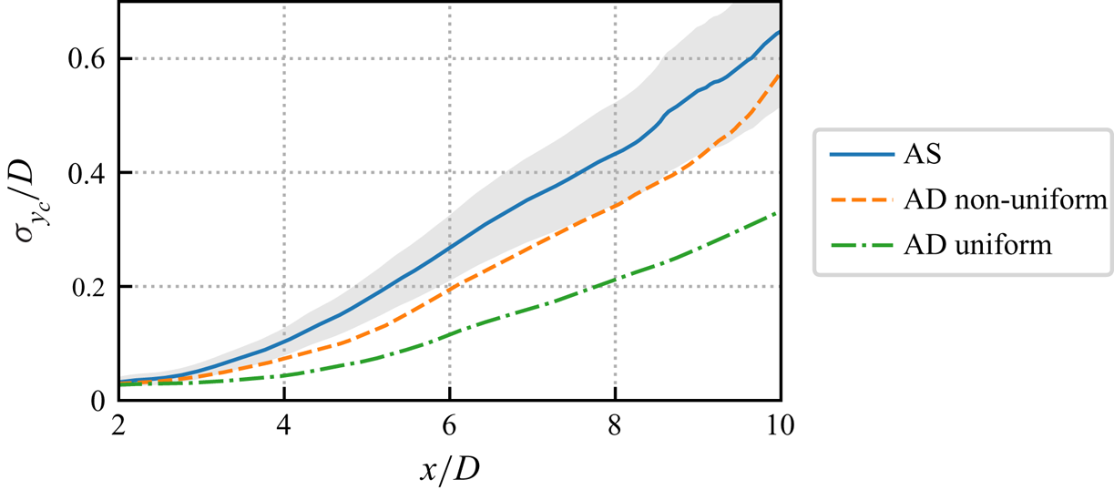
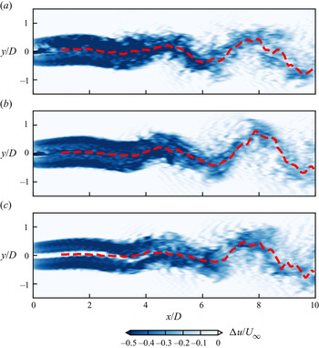
It is also worth noting that the actuator surface model employed in this work requires relatively high computational cost; further work may consider the actuator disk model in both experiments and simulations to simply the turbine modelling. The predictive capability of the actuator disk model for the wake of an oscillating turbine is evaluated in Appendix A.
2.3. Simulation set-up
In the present cases, the NREL offshore 5 MW baseline wind turbine (Jonkman et al. Reference Jonkman, Butterfield, Musial and Scott2009) is employed. It has a rotor with diameter 126 m and a cuboidal shape nacelle ( $2.3\,\text {m} \times 2.3\,\text {m} \times 14.2\,\text {m}$). The simulation represents the rated operation condition with wind speed
 $U_\infty = 11.4\,\text {m}\,\text {s}^{-1}$ and tip speed ratio
 $\lambda = 7$. The Reynolds number based on the inflow velocity and the rotor's diameter is
 $Re \approx 9.6\times 10^7$. Two types of inflows are considered: (i) an idealized uniform inflow to focus only on the effects of side-to-side motion to isolate it from inflow turbulence; (ii) inflows with turbulence and shear to assess their interplay effects.
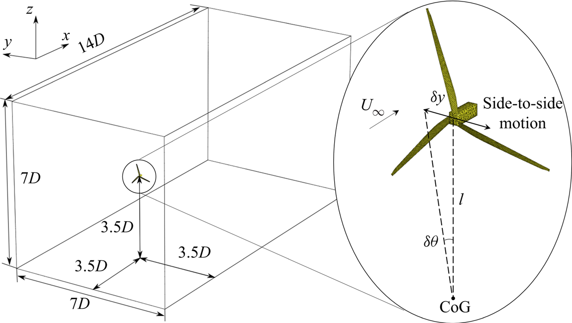
For the cases under uniform inflow without turbulence, the computational domain, shown in figure 1, is a cuboid with  $L_x \times L_y \times L_z = 14D \times 7D \times 7D$, where
 $x$,
 $y$ and
 $z$ denote the streamwise, horizontal and vertical directions, respectively. The turbine is placed
 $3.5D$ from the inlet and located at the centre of the cross-section. The origin of the coordinate system coincides with the wind turbine's hub centre. The inflow velocity is imposed on the inlet boundary at
 $x = -3.5D$. The Neumann condition for velocity (
 $\partial u_i/\partial x=0$) is applied on the outlet boundary at
 $x = 10.5D$. The free slip condition is imposed on the four lateral boundaries. The computational domain is discretized with a Cartesian grid (a degeneration of the curvilinear grid). The streamwise grid is uniform with
 ${\rm \Delta} x = D/20$. In the
 $y$ and
 $z$ directions, the grid spacing is
 ${\rm \Delta} y = {\rm \Delta} z = D/40$ near the wake centreline, i.e. in the region
 $y \times z \in [-1.5D, 1.5D] \times [-1.5D, 1.5D]$. Out of this near turbine region, the grid is gradually stretched in both lateral directions. The total number of nodes is
 $N_x \times N_y \times N_z = 281 \times 141 \times 141 \approx 5.6$ million. Such a grid resolution is fine enough for the actuator model to predict the velocity deficit and turbulence intensity in turbine wakes with reasonable accuracy based on a previous grid refinement study (Yang et al. Reference Yang, Sotiropoulos, Conzemius, Wachtler and Strong2015).
Schematics of the computational domain for cases without wind shear and the rotor side-to-side motion.

In addition to the uniform inflow, cases with inflow turbulence and wind shear are set to investigate their interplay effects with turbine motions. To isolate the effects of turbulence and shear, they are treated separately. For the cases with inflow turbulence only, uniform inflows superimposed with turbulence generated using Mann's synthetic turbulence technique (Mann Reference Mann1998) are employed for six different values of turbulence intensity (TI) – i.e. 0 %, 1.5 %, 3.8 %, 4.7 %, 10.6 %, 15.8 % – which denotes the ratio between the standard deviation of streamwise velocity to its mean ( $\sigma _u/U$). Based on a four-year wind measurement at 45 km offshore, Türk & Emeis (Reference Türk and Emeis2010) reported that for wind speed
 $11\,{\rm m}\,{\rm s}^{-1} < U < 13\,{\rm m}\,{\rm s}^{-1}$, the minimal value of TI is smaller than 1 %, its mean value is approximately 4.5 %, and the 90 % quantile falls at approximately 7–8 %. These cases employ the same computational domain and the same grid as those under uniform inflow.
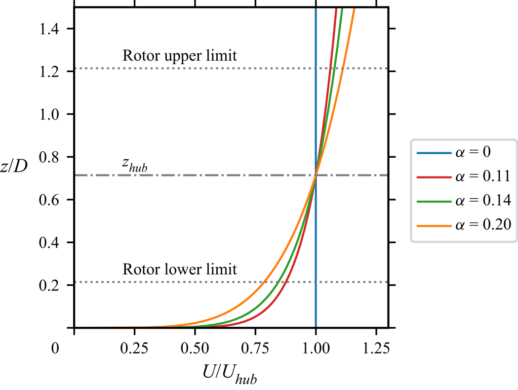
For the cases with vertical wind shear, the vertical profile of the streamwise velocity at the inlet is generated using the power law as
 \begin{equation} U(z) = U_{hub}\left( \frac{z}{z_{hub}} \right)^\alpha, \end{equation}
with different exponential coefficients, i.e.  $\alpha =0$, 0.11, 0.14 and 0.20;
 $\alpha = 0.14$ corresponds to the normal wind condition defined by the IEC standard for offshore wind turbines (IEC 2019), and the other values represent lower and higher wind shear conditions. These profiles are illustrated in figure 2. No velocity fluctuation is added at the inlet boundary. It is noted that turbulence can be produced by the shear in the vertical direction. For the considered cases, the streamwise length of the computational domain is comparable to the thickness of the atmospheric boundary layer, which is not enough for turbulence to become fully developed. The simulation results show that the turbulence intensity
 $\sigma _u/U_\infty$ measured
 $2D$ aside from the hub location is 0.62 %, 0.60 %, 0.59 % for the cases with
 $\alpha = 0.11$, 0.14 and 0.20, respectively, and grows to approximately 1.0 % at
 $8D$ turbine downstream for all the considered non-zero shear exponents. It is worth noting that for the cases with vertical shear, the rotor is placed at (
 $z_{hub}=90$ m) above the ground, such that the grid and the computational domain are different from other cases. In these cases, the grid is modified such that
 ${\rm \Delta} y = {\rm \Delta} z$ are equal to
 $D/40$ in the near ground region
 $z \in (0,2D)$, and
 ${\rm \Delta} z$ is gradually stretched to the top boundary located
 $11.11D$ (1 km) from the ground.
Vertical profiles of the streamwise velocity for the cases under inflow with vertical shear. The velocity distribution is given by the power law with different exponents  $\alpha$.

Each simulation takes about 40 rotor revolutions to fully develop the wake initially. The time series of the total kinetic energy are examined as well to ensure that a statistically steady state is achieved. After this transitional stage, the instantaneous flow fields are saved for further investigation.
2.4. Side-to-side motions
In the simulations, the wind turbine is imposed with a simple harmonic motion in the transverse direction as shown in figure 1. Two independent control variables are employed, i.e. the motion amplitude ( $A$) and the period (
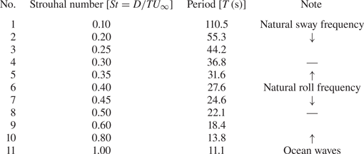
 $T$), with their values listed in tables 1 and 2. The rotor's displacement is defined as
 $\delta y = A \sin (2{\rm \pi} t/T )$.
Amplitudes of the simple harmonic motion of the rotor hub and the corresponding roll motion amplitudes.

The Strouhal numbers and periods of the simple harmonic motions; the last column describes approximately the corresponding ranges of the different physics. The Strouhal number is calculated with the reference velocity  $U_\infty = 11.4\,{\rm m}\,{\rm s}^{-1}$ and rotor diameter
 $D=126\,\textrm {m}$.

In the present work, only motions with relatively small amplitudes are considered, to ensure that the hub acceleration is within the mechanical design requirement (Nejad, Bachynski & Moan Reference Nejad, Bachynski and Moan2019). It is worth noting that such a side-to-side motion can stem from either the translation along the  $y$ axis (the sway motion) or the rotation along the
 $x$ axis (the roll motion) with respect to the centre of gravity (CoG) of the floating wind turbine and the platform. For small roll motion, the side-to-side hub displacement
 $\delta y$ and the roll angle
 $\delta \theta$ can be approximated with
 $\delta y \approx l\,\delta \theta$, where
 $l \approx 100\,\textrm {m}$ is the distance from the hub to the CoG (Robertson et al. Reference Robertson2014). Strictly speaking, the roll motion induces an extra vertical displacement, so it is not fully equivalent to the sway motion. However, such a vertical displacement is rather small for the motion amplitudes considered in this work and it is thus neglected, e.g. the vertical displacement is approximately 0.1 m (
 $<0.001D$) for the case with the largest motion amplitude
 $A = 0.04D$. It is noted that such a side-to-side motion can be triggered by sources such as oblique waves, atmospheric turbulence and the meandering of upstream turbine wakes.
From the wave-structure interaction point of view, the horizontal side-to-side motions of an FOWT can be divided primarily into two groups, i.e. those in the wave frequencies and those at the natural frequencies of the sway or the roll motion (Jonkman & Musial Reference Jonkman and Musial2010; Robertson et al. Reference Robertson2014; Leroy et al. Reference Leroy, Gilloteaux, Lynch, Babarit and Ferrant2019). For this reason, the present work selects a rather large frequency range to analyse the influence of different motions from both groups, as shown in table 2. The high-frequency part corresponds to the motions induced directly by the first-order wave forces, i.e. with periods approximately 10–15 s at operational sea states (Toffoli & Bitner-Gregersen Reference Toffoli and Bitner-Gregersen2017). On the other hand, the natural frequencies, although changing from case to case due to different turbine and platform designs, usually fall into a lower frequency range. For instance, the periods corresponding to the natural frequencies of roll and sway motions are approximately 25–30 s and 100–120 s, respectively, for currently available prototype floating platforms (Jonkman & Musial Reference Jonkman and Musial2010; Robertson et al. Reference Robertson2014). These lower frequencies are also considered in the present work as shown in table 2. It is noted that the tension leg platform (TLP) design may have very short rolling natural periods ( $T<10$ s, corresponding to
 $St>1.0$ for the present rotor design) (Zhao, Yang & He Reference Zhao, Yang and He2012). However, it will be shown in § 3.2 that high-frequency motions contribute little to the far wake meandering.
3. Results
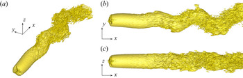
The effects of side-to-side motion on the wake meandering are presented in this section. A typical three-dimensional wake structure is illustrated in figure 3, showing the LES result of the case with  $St = 0.25$ and
 $A/D =0.04$. As can be seen, the wake meandering is essentially two-dimensional, residing primary in the
 $xy$ plane with negligible motion in
 $z$ direction. For this reason, only results on the horizontal plane located at hub height (
 $z = z_{hub}$) are presented hereafter, if not otherwise specified.
Three-dimensional structure of the instantaneous wake for the case with  $St = 0.25$ and
 $A = 0.04D$ illustrated by the velocity iso-surface
 $U = 0.8U_\infty$: (a) perspective view, (b) top view, and (c) side view.

This section consists of three subsections. The first two subsections deal only with the idealized uniform inflow condition to focus on the effect of the FOWT side-to-side motion. Subsection 3.1 presents the case with  $St = 0.25$ and
 $A/D =0.04$ to show the typical wake behaviour of an oscillating FOWT and to introduce the data processing methods employed for extracting wake characteristics. In § 3.2, the influence of motion amplitudes and frequencies is analysed by using both LES data and LSA. Finally, the effects of inflow turbulence and vertical wind shear are addressed in § 3.3.
3.1. Effects of wind turbine oscillations
3.1.1. Instantaneous wake characteristics
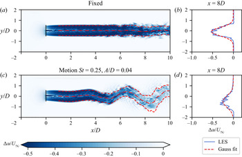
The influence of turbine side-to-side motion on the instantaneous wake is revealed in figure 4, where snapshots of the instantaneous wakes behind a fixed wind turbine and behind an oscillating one are compared. Figures 4(a) and 4(c) compare the contours of the instantaneous streamwise velocity deficit with the centreline and width of the wake extracted with a Gaussian fit defined as
 \begin{equation} {\rm \Delta} u(x,y) = u(x,y) - U_\infty = {\rm \Delta} u_c(x) \exp{\left(-\frac{(y-y_c(x))^2}{2 s^2(x)}\right)}, \end{equation}
where  $u(x,y)$ is the streamwise velocity and
 $s(x)$ is the standard deviation of the Gaussian distribution to be fitted with the velocity profile. The wake centre position
 $y_c$ is defined with the peak of the Gaussian fit, and is plotted with red dash-dotted lines. The wake width (red dashed lines) is defined as
 $r_{1/2}(x) = \sqrt {2\ln 2} s(x)$, which gives the distance from
 $y_c(x)$ to the position where
 ${\rm \Delta} u = \frac {1}{2}{\rm \Delta} u_c$. This fitting technique based on self-similarity, which is often applied to extract the features of time-averaged wakes (Xie & Archer Reference Xie and Archer2015; Bastankhah & Porté-Agel Reference Bastankhah and Porté-Agel2016), has been demonstrated as being able to extract features of instantaneous wakes (Li & Yang Reference Li and Yang2021), especially when the inflow turbulence is subtracted. Other methods – e.g. calculating the instantaneous wake centre position
 $y_c$ as the weight centre of
 ${\rm \Delta} u$ (Bastankhah & Porté-Agel Reference Bastankhah and Porté-Agel2017) or
 ${\rm e}^{-{\rm \Delta} u}$ (Muller et al. Reference Muller, Aubrun and Masson2015) – have been also employed when inflow turbulence presents.
Instantaneous streamwise velocity deficit in the wake behind a fixed wind turbine (a), and a wind turbine subject to side-to-side simple harmonic motion with  $St = 0.25$ and amplitude
 $A/D = 0.04$ (c). The wind turbines are illustrated with black solid lines. The red dash-dotted lines and the dashed lines indicate the centrelines and the wake width, respectively. They are obtained with the Gaussian fit of the velocity deficit profile, as shown in (b,d) for the wakes of the fixed wind turbine and the moving wind turbine, respectively.

As can be seen in figure 4(a), the centreline of the wake behind the fixed wind turbine is approximately straight in the near wake and fluctuates mildly in the far wake ( $x>6D$). Moreover, the width of the wake behind the fixed turbine remains almost constant at all downstream locations, suggesting that the wake recovery is slow for the fixed turbine for the simulated case without inflow turbulence. In contrast, the oscillating wind turbine generates a wake with large-amplitude oscillations as shown in figure 4(c), revealing a significant impact of the side-to-side motion on turbine wakes. The meandering amplitude is found to be comparable to the turbine diameter in the far wake, while the amplitude of the side-to-side motion is only
 $A = 0.04D$. This rapid growth shows that the initial perturbation induced by the turbine motion is vastly amplified as one travels downstream. Besides the wake centreline oscillation, the velocity deficit in the far wake is also significantly affected, being weaker behind the oscillating turbine when compared with the fixed turbine as shown in figures 4(a) and 4(c). This difference is more evident in figures 4(b) and 4(d), where the transverse profiles of the velocity deficit at downstream location
 $x=8D$ are plotted. The blue curves represent the instantaneous velocity deficit, and the red dashed lines are their Gaussian fits defined with (3.1). It is clear that the centreline velocity deficit
 ${\rm \Delta} u_c$ is stronger and the wake width is narrower for the fixed wind turbine when compared with the oscillating wind turbine. As for the distribution of the velocity deficit, the wake behind the fixed turbine is symmetric and can be fitted well with the Gaussian curve. The wake of the oscillating wind turbine, on the other hand, shows obvious asymmetry. Despite the observed asymmetry, the essential features of the meandering wake – i.e. the centreline position, the velocity deficit and the width – are well captured by the Gaussian fitting. It is worth noting that these instantaneous wake profiles deform from one instant to another, especially in the meandering case. Further investigation on the time-averaged wake profile in the frame of references fixed in space and following the meandering wake centre will be provided in §§ 3.1.2 and 3.1.3, respectively.
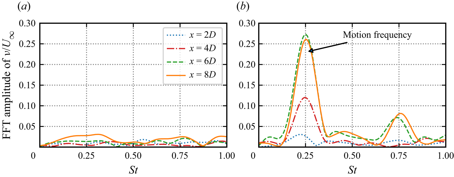
The wakes downstream of the fixed and the oscillating wind turbines are further compared by examining the frequency spectra of the spanwise velocity fluctuations in figure 5, which are computed with instantaneous spanwise velocities ( $v$) recorded along the time-averaged wake centreline (
 $y=0$) at four turbine downstream locations (
 $x = \{2D,4D,6D,8D\}$) using the discrete Fourier transform. As shown in figure 5(a), the velocity behind the fixed wind turbine contains only small-scale fluctuations, which are influenced by the hub vortex in the wake of the nacelle and are distributed over a wide range of frequencies. No obvious growth can be found for the fluctuation amplitude as one travels downstream. In contrast, the spectra behind the oscillating wind turbine consist of a distinct peak at the frequency of the imposed motion (
 $St=0.25$). Moreover, the fast Fourier transform (FFT) magnitude at
 $St=0.25$ grows significantly with downstream distances, revealing the onset of the instability of the wake, which significantly amplifies the disturbances initiated by the side-to-side motion. The FFT magnitude at other frequencies remains approximately the same except at three times the imposed frequency. It is also observed that the amplitude at the imposed frequency ceases to grow from
 $x=6D$ to
 $x=8D$, while the peak at a higher frequency (
 $St \approx 0.75$) starts to appear at
 $x=6D$, which indicates the saturation of the linear growth process and the energy transfer from low to high frequencies via nonlinear effects. According to the stability theory (Schmid, Henningson & Jankowski Reference Schmid, Henningson and Jankowski2002; Drazin & Reid Reference Drazin and Reid2004), nonlinear effects result in energy growth at the sum and difference frequencies of the base perturbation, so that the second harmonic (
 $St = 0.25 +0.25 = 0.5$) appears first, then it interacts with the first harmonic (
 $St=0.25$) to generate the third harmonic (
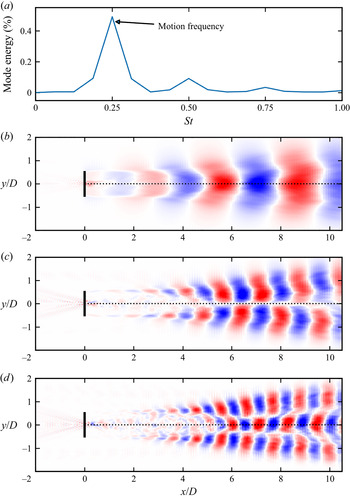
 $St=0.5+0.25=0.75$). The absence of the second harmonic on the wake centreline, which seems to contradict this theory at first glance, is related to this specific location, i.e. the wake centreline. To show this, we plot the coherent structures of the whole wake revealed by the spectral proper orthogonal decomposition (SPOD) (Towne, Schmidt & Colonius Reference Towne, Schmidt and Colonius2018) in figure 6. As can be seen in figure 6(a), an energy concentration does exist at the second harmonic (
 $St = 0.50$). Interestingly, its coherent structure, as shown in figure 6(c), is approximately anti-symmetric with very weak velocity fluctuations near the centreline, which explains why the FFT magnitude computed based on the centreline velocity fluctuations has no apparent component at
 $St = 0.50$ as shown in figure 5(b). In contrast, the first and third harmonics, appearing in the spectra of the centreline velocity fluctuation, both have symmetrical spatial modes (figure 6b,d)
Fast Fourier transform (FFT) amplitude of the normalized spanwise velocity ( $v/U_\infty$) in the wake behind the fixed wind turbine (a), and the wind turbine subject to side-to-side FOWT motion with
 $St = 0.25$,
 $A/D=0.04$ (b). Data are collected at four downstream locations (
 $x = \{2D,4D,6D,8D\}$) along
 $y=0$.

Spectral proper orthogonal decomposition (SPOD) of the wake of an FOWT oscillating at  $St = 0.25$, the normalized modal energy as a function of Strouhal number (a), the principal SPOD mode of the transverse velocity
 $v$ of the first harmonic
 $St = 0.25$ (b), the second harmonic
 $St = 0.50$ (c), and the third harmonic
 $St = 0.75$ (d).

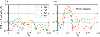
Similar to the above analyses, the spectra of the wake centre displacement is computed and shown in figure 7. It is observed that the amplitudes of the wake centre oscillations behind the oscillating wind turbine are one to two orders of magnitude higher than those of the fixed wind turbine at the frequency of the imposed side-to-side motion. For other frequencies, the FFT magnitudes from the oscillating wind turbine are comparable to those of the fixed wind turbine, which does not have any distinct peak frequencies. Furthermore, it is observed that the FFT magnitude at the peak frequency grows monotonically as one travels downstream from the turbine and is comparable to the rotor diameter in the far wake ( $x=6D, 8D$).
FFT amplitude of the normalized wake centre displacement  $y_c/D$ behind the fixed wind turbine (a) and the wind turbine subject to side-to-side FOWT motion at
 $St = 0.25$,
 $A/D=0.04$ (b). Data are collected at four downstream locations (
 $x = \{2D,4D,6D,8D\}$) along
 $y=0$.

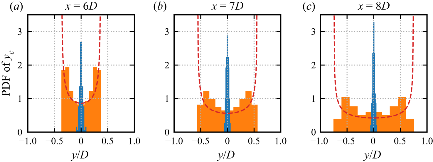
Another interesting observation is that the spanwise distribution of instantaneous wake centre positions becomes very different for the oscillating turbine when compared with the fixed one. These instantaneous wake centres are sampled from instantaneous flow fields at evenly distributed time steps. In figure 8, the probability density functions (PDFs) of instantaneous wake positions at turbine downstream locations  $x=6D, 7D, 8D$ are compared. It is found that the PDF for the wake centres of the fixed wind turbine approximately follows the normal distribution located in a very narrow band, which barely changes as one moves downstream, being consistent with the instantaneous wake shown in figure 4(a). In contrast, the PDF of instantaneous wake centres behind the oscillating wind turbine spreads much wider and expands as one travels downstream. More importantly, the PDF shows a distinct pattern, with two peaks near the two extremities and a trough near
 $y=0$, which is significantly different from that observed for the fixed wind turbine and that of wake meandering induced by inflow turbulence, whose PDFs are approximately Gaussian (Li & Yang Reference Li and Yang2021). In contrast, this PDF is close to that of a simple harmonic motion (red dashed line), with a trough around the equilibrium position and two peaks at extremities (Tennekes & Lumley Reference Tennekes and Lumley1972). This is expected as the turbine side-to-side motion is imposed with a harmonic function as well. More importantly, the differences between the PDF of the wake centres of an oscillating turbine and that of a simple harmonic motion should be noticed, namely that the two peaks near the two extremities move quickly towards the centre as one moves to further turbine downstream locations. From the practical point of view, this PDF implies that the wake of an oscillating wind turbine may partially shelter the downstream turbine more often than a fixed wind turbine.
Probability density functions of wake centre positions  $y_c$ at turbine downstream locations
 $x=6D, 7D, 8D$ for the fixed wind turbine (blue) and the oscillating wind turbine (orange) with
 $St = 0.25$,
 $A/D=0.04$. The PDF of the fixed wind turbine is multiplied by a factor of
 $1/5$ to plot them in the same figure. The red dashed lines show the PDF of an idealized harmonic motion with the amplitude defined by the extremity of
 $y_c$ of the oscillating wind turbine case.

3.1.2. Time-averaged wake in the meandering frame of reference
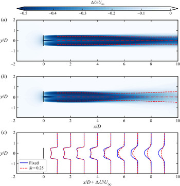
With the instantaneous wake centre positions tracked with the Gaussian fit method, wake characteristics on the meandering frame of reference (MFR) are studied, as in Trujillo et al. (Reference Trujillo, Bingöl, Larsen, Mann and Kühn2011). Figure 9 plots the velocity deficits ensemble-averaged on the MFR for both fixed and side-to-side oscillating cases. As can be seen, the ensemble-averaged velocity deficits are approximately symmetric with respect to the wake centreline for both cases. In the near wake (until  $x=3D$ turbine downstream), it is observed that the velocity deficit profiles from the side-to-side oscillating case are almost the same as those from the fixed case, as shown in figure 9(c). Differences are observed at further downstream locations, where the wake behind the oscillating rotor recovers more rapidly and expands slightly wider, being consistent with the observation of the instantaneous velocity as shown in figure 4. For instance, at the
 $x = 8D$ turbine downstream, the wake centreline velocity deficits are
 ${\rm \Delta} u_c = -0.27 U_\infty$ and
 ${\rm \Delta} u_c = -0.50 U_\infty$ for cases with/without rotor oscillation, respectively. Such differences between the two cases increase with turbine downstream distance, indicating a stronger influence of wake meandering on wake recovery at far wake locations.
Time-averaged wake deficit in the meandering frame of reference for the fixed turbine case (a) and the oscillating turbine case with  $St = 0.25$ and
 $A/D = 0.04$ (b). The velocity deficit profiles are compared in (c). The dash-dot lines and the dashed lines in (a,b) illustrate the fitted wake centreline and the wake half-width, respectively.

The turbulence intensity defined in the meandering frame of reference is examined in figure 10, which is defined as
 \begin{equation} \text{TI} = \sqrt{\frac{2k}{3}}/U_\infty, \end{equation}
where  $k$ is the turbulence kinetic energy
 $k = \frac {1}{2}(u'^2 + v'^2 + w'^2)$. It is noticed that
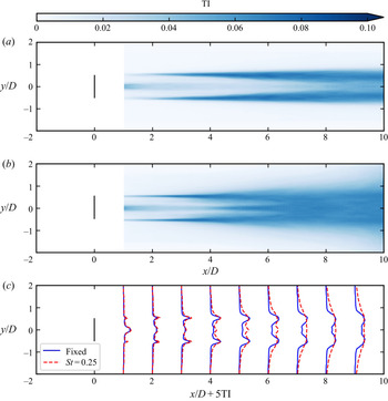
 $u^{\prime },v^{\prime },w^{\prime }$ are the root-mean-square of the fluctuations of the three velocity components defined with respect to the mean velocity averaged on the meandering frame of reference. As can be seen, the TI profiles have two peaks near the wake boundaries and gradually expand inwards and outwards for both cases. Such expansion is faster in the oscillating turbine case. At
 $x\ge 7D$, the two peaks of TI merge as one on the centreline for the oscillating turbine case, which is retained for the fixed case even at the
 $x=9D$ turbine downstream. The maximum TI is approximately the same for both cases, at approximately
 $6.8\,\%$ at
 $x=8D$ for both cases, while the distribution of TI is much wider for the oscillating turbine case.
Time-averaged rotor added turbulence intensity in the meandering frame of reference for the fixed rotor case (a) and the moving rotor case with  $St = 0.25$ and
 $A/D = 0.04$ (b). The turbulence intensity profiles from both cases are compared in (c).

3.1.3. Time-averaged wake in fixed frame of reference
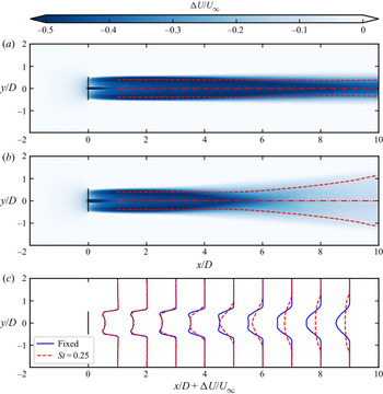
The effects of turbine motion on the time-averaged wake are examined in this subsection in the ground fixed frame of reference (FFR). First, we show the contour of streamwise velocity deficit in figure 11. It is observed that the time-averaged velocity deficits of the fixed and oscillating turbine cases are close to each other in the near wake region ( $x<3D$). At further downstream locations, the wake of the fixed wind turbine as shown in figure 11(a) shows only a mild expansion, and the shear layer grows gradually in both inward and outward directions. The maximum deficit along the wake centreline remains approximately
 ${\rm \Delta} U = U- U_\infty = -0.49 U_\infty$ at
 $x=8D$. By contrast, the wake behind the oscillating wind turbine as shown in figure 11(b) shows an obvious broader wake expansion starting from
 $x=4D$, as a result of large-amplitude meandering motion, which spreads the low speed region to a larger extent. A direct result of this broad wake expansion is the faster recovery of momentum deficit in the wake core. As shown in figure 11(c), the time-averaged velocity deficit is approximately
 ${\rm \Delta} U \approx -0.18U_\infty$ at
 $x=8D$, being significantly lower than that behind the fixed wind turbine (
 ${\rm \Delta} U \approx -0.49U_\infty$). This deficit of the oscillating turbine is also weaker than
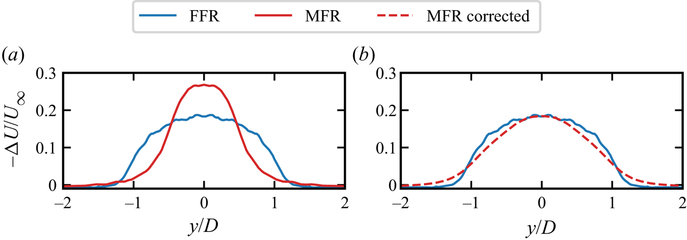
 ${\rm \Delta} u_c = -0.27U_\infty$ in the MFR, as shown in figure 12(a). The differences between the velocity deficits on the FFR and MFR are found to be much reduced by taking the meandering motion into account, as shown in figure 12(b), where
 ${\rm \Delta} U$ in the FFR shows a good agreement with the weighted averaged of
 ${\rm \Delta} U$ in the MFR using the wake centre PDF plotted in figure 8.
Time-averaged streamwise velocity deficit in the fixed frame of reference in the wake behind a fixed wind turbine (a) and a wind turbine subject to side-to-side simple harmonic motion with  $St = 0.25$ and amplitude
 $A/D = 0.04$ (b), and a comparison of velocity deficit profiles for both cases in (c).

Comparison between the time-averaged velocity deficit profile in the fixed frame of reference (FFR) and the meandering frame of reference (MFR) at  $x=8D$ for the case with
 $St=0.25$ and
 $A=0.04D$: (a) velocity deficits in both frames of references compared directly, (b) comparison of the velocity deficit in the MFR corrected with the PDF of wake centre locations with that in the FFR.

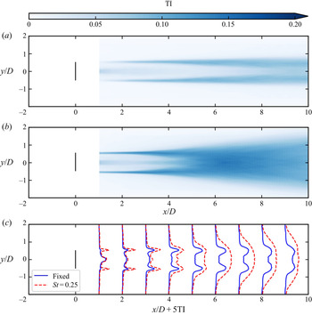
Except for the benefit of the faster wake recovery, the wake meandering also results in stronger unsteady loads for the downstream turbines, which is unfavourable for the structure of the downstream turbines. The obtained contours and profiles of the TI are shown in figure 13. As expected, the oscillating motion of the wind turbine has drastically intensified the turbulence intensity in the wake in terms of both magnitude and spatial extent. Specifically, it is observed that the TI behind the hub and the tip of the rotor is intensified in the near wake because of turbine oscillation. Starting from  $x=2D$, the TI grows in the shear layer of the wake and extends both inward to the wake core and outward to the freestream as one travels downstream. At approximately
 $x=5D$, the shear layers from the tips meet at the wake centre for the oscillating turbine case. At further turbine downstream locations, the TI ceases to grow and slightly decreases, starting from
 $x=7D$. At
 $x=8D$, the TI in the oscillating turbine case is significantly higher than that in the fixed turbine case (maximum TI
 $\approx$ 13.4 %, 8.5 % for the two cases, respectively). It is noticed that this level of turbulence intensity is within the range of the wind turbine design standard (
 $\textrm {TI}_{ref} = 14\,\%$ for turbulence category B as per IEC 61400-1).
Turbulence intensity (TI) in the ground fixed frame of reference of the wake behind a fixed wind turbine (a) and a wind turbine subject to the side-to-side harmonic motion ( $St = 0.25$ and
 $A/D = 0.04$) (b). The transverse profiles of TI in both cases are compared in (c).

3.2. Effects of motion frequencies and amplitudes
After showing the results from a specific case, in this subsection we perform local LSA and carry out simulations with a series of frequency and amplitude combinations to examine how the onset of wake meandering depends on these control parameters.
3.2.1. Local linear stability analysis
Previous studies on wind turbine wakes in the literature have demonstrated their convective instability (Iungo et al. Reference Iungo, Viola, Camarri, Porté-Agel and Gallaire2013; Sarmast et al. Reference Sarmast, Dadfar, Mikkelsen, Schlatter, Ivanell, Sørensen and Henningson2014; Mao & Sørensen Reference Mao and Sørensen2018; Gupta & Wan Reference Gupta and Wan2019), i.e. the wake behaves as an amplifier of upstream disturbances. For a prescribed base flow, the linear stability theory can predict the spatial amplification rate for an infinitely small disturbance at different excitation frequencies. In the following, a local LSA is performed to assess the response of the wake to small disturbances with different frequencies. The time-averaged flow behind a fixed wind turbine is simplified using locally axis-parallel and axisymmetric assumptions, i.e. the velocity is simplified as  $(\bar U(r,x),0,0)$ in the streamwise, radial and azimuthal directions (where
 $\bar {U}$ is the temporally and azimuthally averaged streamwise velocity), and employed as the base flow for the LSA. The perturbation velocity components
 $(u_x,u_r,u_\theta )$ and the perturbation pressure
 $p$ are assumed to be the form
 $(u_x,u_r,u_\theta,p) = (\hat {u}_x,\hat {u}_r,\hat {u}_\theta,\hat {p}) (\exp ({\rm i}k x + {\rm i}n\theta - {\rm i}\omega t) )$, where
 $\hat {\cdot }$ denotes the shape function in the radial direction and
 $n$ is the azimutal wave number of the perturbation mode. For the cases considered in the present work, the azimuthal wave number is equal to one, i.e.
 $n=1$, as the side-to-side motion velocity (
 $u_y$) can be projected in the radial and azimuthal directions as
 $u_r = u_y \cos \theta$ and
 $u_\theta = u_y \sin \theta$. Spatial stability analyses are performed with angular frequency
 $\omega = 2{\rm \pi} f$ (real number) and wavenumber
 $k=k_r+{\rm i}k_i$ (complex number). Substituting the perturbation variables into the linearized Navier–Stokes equations yields
 \begin{gather} {\rm i} k \hat{u}_x + \frac{\hat{u}_r}{r} + \frac{{\rm d} \hat{u}_r}{{\rm d} r} + \frac{{\rm i} n \omega}{r}\,\hat{u}_\theta = 0, \end{gather}
 \begin{gather}{\rm i} ( k \bar{U} -\omega ) \hat{u}_x + \frac{{\rm d} \bar{U}}{{\rm d} r}\,\hat{u}_r ={-} {\rm i} k \hat{p}, \end{gather}
 \begin{gather}{\rm i} ( k \bar{U} - \omega ) \hat{u}_r ={-} \frac{{\rm d} \hat{p}}{{\rm d} r}, \end{gather}
 \begin{gather}{\rm i} ( k \bar{U} - \omega ) \hat{u}_\theta ={-} \frac{{\rm i} n}{r}\,\hat{p}. \end{gather}
The above equations are the same as those derived by Batchelor & Gill (Reference Batchelor and Gill1962) for axisymmetric jets/wakes, except that the viscous terms are excluded, because their contribution is less important for base flow velocity profiles with inflection points (Schmid et al. Reference Schmid, Henningson and Jankowski2002). The linearized Navier–Stokes equations are discretized with Chebyshev polynomials on  $128$ Gauss–Lobatto nodes
 $\xi \in [-1,1 ]$ and stretched to
 $r \in [0, r_{max}]$ through an algebraic mapping (Schmid et al. Reference Schmid, Henningson and Jankowski2002) defined as
 $r = a ({(1+\xi )}/{(b-\xi )})$ with
 $a = {r_{max}}/{(r_{max}-2)}$ and
 $b=1+{2a}/{r_{max}}$. The size of the computational domain is chosen as
 $r_{max} = 15D$. The size of the domain and the number of discretization points are verified to be large enough to not affect the stability analyses. The far field boundary condition is that the perturbations vanish at
 $r = r_{max}$. On the wake centreline,
 $\hat {u}_x = 0$,
 $\hat {p}=0$ and
 $\hat {u}_r + i \hat {u}_{\theta } = 0$ are imposed following Batchelor & Gill (Reference Batchelor and Gill1962).
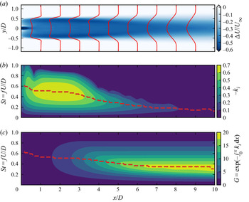
Figure 14 shows the results of local LSA conducted at different downstream locations. As can be seen in figure 14(a), the velocity deficit profiles in the region between the core of the wake and the freestream is characterized by a shear layer. The thickness of this shear layer gradually increases in the turbine downstream direction due to the momentum mixing between the wake and the freestream, and consequently makes the local stability properties vary with the downstream distance as shown in figure 14(b). In the near wake ( $x<3D$), the steep velocity variation in the shear layer results in a broad range of unstable frequencies
 $St \in (0, 0.9)$ approximately, with the most unstable frequency at
 $St \approx 0.5$. At further turbine downstream locations, both the most unstable frequency and the range of the unstable frequencies decrease. This trend of decrease of the most unstable frequency via the downstream distance is in agreement with the work of Gupta & Wan (Reference Gupta and Wan2019), where LSA is applied to the time-averaged wake of a tidal turbine. Such downstream variations of the spatial growth rate indicate that perturbations that are the most unstable in the near wake become stable when propagating downstream and cease to grow subsequently. On the other hand, perturbations at lower frequencies may excel in the far wake since they can grow for a longer distance. To demonstrate this accumulation effect via downstream distances, figure 14(c) displays the contours of the integrated amplification factor defined as
 $G =\exp {(-\int _0^x k_i \,\textrm {d}\kern0.7pt x)}$. As expected, it is found that the frequency with the largest amplification factor
 $G$, shown with the red dashed line, also decreases in the streamwise direction until approximately
 $x=7D$. In the far wake, perturbations with evident amplifications fall in the frequency range
 $0.1< St<0.8$. The strongest amplification factors are predicted for
 $0.2< St<0.4$, explaining the large-amplitude wake meandering triggered by turbine side-to-side motion with
 $St=0.25$ as presented in § 3.1. Furthermore, this frequency range is rather low compared to the commonly encountered excitement frequencies generated by wind turbines, e.g. the rated rotor frequency and the blade passing frequency are approximately equal to
 $0.2\,\textrm {Hz}$ (
 $St \approx 2.2$) and
 $0.6\,\textrm {Hz}$ (
 $St \approx 6.6$), respectively, for the NREL 5 MW wind turbine (Jonkman et al. Reference Jonkman, Butterfield, Musial and Scott2009) as well as other wind turbines at utility scale. As a result, unstable modes of the wake are unlikely to be triggered by the rotation of blades alone, being consistent with the literature that the hub vortex at lower frequencies plays an important role in triggering the shear layer instability and the far wake meandering for the bottom-fixed turbine (Kang et al. Reference Kang, Yang and Sotiropoulos2014). Moreover, this range is also lower than the wave frequencies at operational sea states (
 $St \approx 1.0$) as shown in table 2, indicating that floating wind turbines moving at wave frequencies cannot trigger significant wake meandering. On the other hand, this low frequency range (
 $0.2< St<0.4$) overlaps partially with the natural frequencies of the roll or sway motions as shown in table 2. However, it is noted that the Strouhal numbers computed as
 $St = D/(TU_\infty )$ shown in table 2 are based on the diameter
 $D = 126$ m and the rated wind speed
 $U_\infty = 11.4$ m s
 $^{-1}$ of the NREL 5 MW wind turbine, thus may vary for other turbine designs and wind speeds.
Local linear stability analysis results of the wake behind the fixed wind turbine: (a) the streamwise velocity deficit obtained from large-eddy simulations is employed as the base flow for the linear stability analysis; (b) contours of local spatial growth rate  $-k_i$; and (c) the integrated amplification factor
 $G = \exp {(- \int _0^x k_i \,\textrm {d}\kern0.7pt x)}$. The red dashed lines in (b,c) indicate the most amplified frequency along the streamwise locations.

Although the above LSA can provide useful information on the instability properties of the wake, it is worth noting that the analyses are carried out based on several assumptions for the base flow and the disturbances, i.e. (i) the axis-parallel and axisymmetric assumption for the base flow, (ii) the small perturbation assumption for linearizing the Navier–Stokes equations, and (iii) the inviscid flow assumption. Often, these prerequisites are not fully satisfied in real applications, where the base flow is more complex and the disturbances are of finite amplitudes, such that nonlinear effects may manifest. To further investigate the wake characteristics and to verify the results from the LSA, results from LES cases with the frequencies and amplitudes presented in tables 1 and 2 will be analysed in the following subsections.
3.2.2. Instantaneous wake
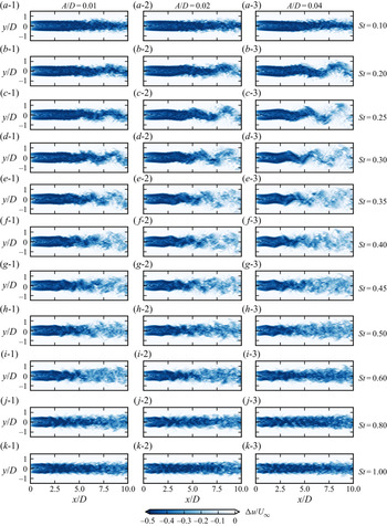
Snapshots of the instantaneous streamwise velocity deficits are plotted for comparison in figure 15. As observed, the wake behaviour varies via the turbine oscillation frequency, being consistent with the LSA. For cases with the lowest and highest motion frequencies, i.e. for  $St = 0.1$ and
 $St \ge 0.8$, no apparent wake meandering is observed, and the wake is almost straight. For the cases with the lowest motion frequency (
 $St = 0.1$), the spanwise motion of the wake is very mild and the wake is close to that behind a fixed turbine. Although increasing the amplitude of the side-to-side motion to
 $A/D=0.04$ can deform the wake slightly into a sinusoidal form, the amplitude of the wake centre displacement is still much smaller than the wake width. For cases with the largest frequencies (
 $St \ge 0.8$), the wake centreline is approximately straight, indicating that the overall meandering motion of the wake is negligible. On the other hand, small-scale fluctuations are observed on the wake boundary, which, however, do not show apparent amplifications as one travels downstream, and remain locally near the boundary without apparent interactions with the core of the wake. Moreover, it is observed that these small-scale fluctuations do not seem to grow in magnitude when increasing the amplitude of the side-to-side motion for which roughly the same instantaneous wakes are observed for cases at
 $St \ge 0.8$ with different amplitudes. In contrast, the cases with
 $0.20 \le St \le 0.60$ show a much stronger far wake meandering, which is consistent with the larger amplification factor predicted by the LSA. Specifically, the cases with
 $0.20 \le St \le 0.40$ exhibit apparent sinusoidal form deformations with a continuous growth of the wake meandering amplitude via the downstream distance until the far wake. Larger meandering amplitudes are also observed when the motion amplitude is increased. For cases with higher Strouhal numbers (
 $0.4 < St \le 0.6$), however, the sinusoidal deformation of the wake is limited only in a certain near-wake region, beyond which the sinusoidal shape wake structures can no longer be identified visually, and the effects of motion amplitude on the wake meandering are hard to tell directly from these instantaneous snapshots.
Instantaneous streamwise velocity deficit behind a wind turbine subject to side-to-side simple harmonic motion for various frequencies and amplitudes. Figures in the same row have the same motion frequency, denoted by the Strouhal number given in the last column. Figures in the same column have the same motion amplitude.

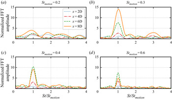
The frequency characteristics of the oscillating wake motion are further examined with the spanwise velocity along the wake centreline as shown in figure 16. In this figure, the spanwise velocity  $v$ is converted into the frequency domain with FFT to obtain the FFT amplitude
 $\phi _v$, which is then normalized by the magnitude of the turbine oscillating velocity
 $\phi _v^0 = 2{\rm \pi} f A$ to indicate the amplification effect of turbine wake. As can be seen, the peak frequencies of
 $\phi _v$ coincide with the turbine motion frequency for all cases, whereas the magnitudes of the peaks (indicating the amplification ratio of the spanwise velocity) vary with the motion frequency. The largest amplification is achieved at
 $x=8D$ for the case with motion frequency
 $St=0.3$. The peak at the three-times frequency is also observed for the case with motion frequency
 $St=0.3$ (figure 16b), but is not apparent for other motion frequencies (figure 16a,c,d). These observations are consistent with instantaneous flow fields shown in figure 15. For the case with low motion frequency, i.e.
 $St=0.2$, the meandering motion just starts even at
 $x/D=8$, and needs more downstream evolution for the nonlinear effect to become evident. For the cases with high motion frequency, i.e.
 $St=0.4$, 0.6, on the other hand, the sinusoidal shape pattern exists for only a short distance, and the wake transits to a chaotic pattern shortly, such that it is hard to distinguish the nonlinear interaction between frequencies.
FFT amplitude of the spanwise velocity  $\phi _v$ normalized by
 $\phi _v^0$ the turbine's oscillating velocity amplitude at
 $y=0$ for different turbine motion frequencies. The amplitude of motion is
 $A=0.01D$.

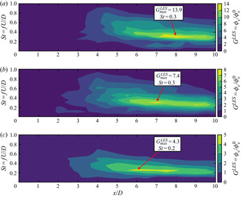
We compute the amplification factor of the spanwise velocity in the wake for different turbine oscillation frequencies and amplitudes, as shown in figure 17. The amplification factor is defined as  $G^{LES} = \phi _v/\phi _v^0$, with
 $\phi _v$ the amplitude of the spanwise velocity at the turbine motion frequency. The amplification factors at every
 $0.5D$ for
 $x\in [0D, 10D]$ are computed. The obtained amplification factors are presented in figures 17(a), 17(b) and 17(c) for the cases with turbine motion amplitudes
 $A/D=0.01, 0.02, 0.04$, respectively. As can be seen, all three figures show a similar pattern. It is observed that the amplification of the spanwise velocity is the most intensive for turbine motions with
 $St \in [0.2,0.3]$ and gradually weakens for lower or higher frequencies. For the cases with the smallest turbine motion amplitude, i.e.
 $A = 0.01D$ in figure 17(a), the location and size of the region with high amplification factors are closer to those predicted by the local LSA (as shown in figure 14c) when compared with the cases with higher oscillation amplitudes. In terms of the magnitudes of the amplification factors, the LES predictions are observed as being, in general, lower than the LSA predictions, because the hypotheses employed in LSA – i.e. the infinite small perturbation, axis-parallel base flow and inviscid fluid – are not fully satisfied. Moreover, it is observed that the differences between LSA and LES predictions are enlarged with increasing turbine motion amplitudes as shown in figures 17(b) and 17(c), which suggests that the nonlinearity caused by the finite-size perturbations plays a role in reducing the growth rate, being consistent with nonlinear stability theory (Schmid et al. Reference Schmid, Henningson and Jankowski2002) and a previous work on tidal turbine wakes (Gupta & Wan Reference Gupta and Wan2019). Furthermore, figure 17 shows that the increase of turbine motion amplitudes slightly lowers the most amplified frequency and narrows the region with high amplification factors.
Contours of the amplification factor  $G^{LES}$ computed from the LES results for different turbine motion amplitudes: (a)
 $A/D =0.01$, (b)
 $A/D=0.02$, (c)
 $A/D = 0.04$. The amplification factor is defined as
 $G^{LES} = \phi _v/\phi _v^0$, where
 $\phi _v$ is the amplitude of spanwise velocity in the wake obtained with the discrete Fourier transform of the time series of the spanwise velocity obtained from LES along the time-averaged wake centreline, and
 $\phi _v^0 = 2{\rm \pi} f A$ is the velocity amplitude of the wind turbine's simple harmonic motion. The largest amplification factor is marked together with its Strouhal number.

3.2.3. Time-averaged wake
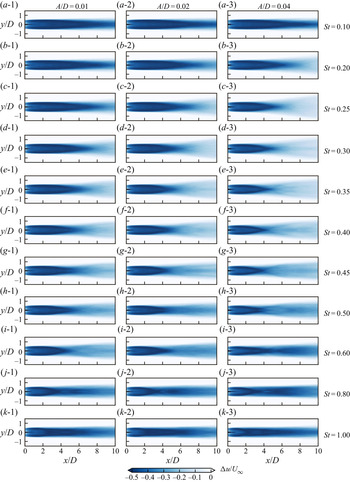
To investigate the influence of turbine motion on the wake recovery, we analyse the time-averaged velocity deficits computed from different cases. In figure 18, we show contours of the time-averaged streamwise velocity deficits. As can be seen, the recovery of the time-averaged wake for cases with  $St = 0.1$ and
 $St \ge 0.8$ is slow, and the wake is close to that of a fixed wind turbine. In contrast, the velocity deficit contours are significantly altered for cases with motion frequencies in the range
 $0.20 \le St \le 0.60$. One interesting observation is that the time-averaged wake recovery is not always enhanced by increasing the turbine motion amplitude as one may expect. One example is the cases with
 $St = 0.6$ (figures 18i-1,i-2,i-3), where the wake recovers slower for
 $A/D = 0.04$ than for
 $A/D = 0.01$.
Time-averaged streamwise velocity deficit at the hub-height plane. The wind turbine is subject to side-to-side simple harmonic motion defined with various frequencies and amplitudes. Figures in the same row have the same motion frequency, denoted by the Strouhal numbers given in the last column. Figures in the same column have the same motion amplitude.

The effect of turbine motion on wake recovery is further examined by the quantitative comparison shown in figure 19, where the velocity deficit averaged over one rotor diameter in the spanwise direction is displayed. In general, it is found that the velocity in the wake recovers faster for an oscillating turbine (lines in colour) than for a fixed turbine (the black line), except when the motion frequency is low ( $St = 0.1$). It is also found that wakes with different turbine motion frequencies respond differently when increasing the motion amplitude. For cases with relative low motion frequencies (
 $St=0.2, 0.25, 0.3$), larger motion amplitudes enhance the wake recovery. The opposite is found for the far wakes in the cases with motion frequency
 $St \ge 0.5$, where wake recovery slows down when the motion amplitude is increased. For the cases with
 $St = 0.4$, wake recovery is almost the same for all three amplitudes, if focusing on
 $\widetilde {{\rm \Delta} U}$ at
 $x=10D$.
Velocity deficit averaged in time and in space (over one rotor diameter) for cases with different turbine oscillation frequencies and motion amplitudes.

3.2.4. Wake turbulence
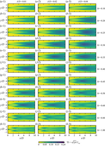
Figure 20 displays the contours of the turbulence intensity in the fixed frame of reference on the hub-height plane for cases with different motion amplitudes and frequencies. It is worth noting that the turbulence intensity compared in this subsection also considers the velocity fluctuations due to the large-amplitude wake meandering. A distinct separation of the two types of velocity fluctuations as done in figure 13 is not straightforward here, especially for cases with high motion frequencies where the meandering is hard to define. As can be seen, the cases with high turbulence intensity are those with large-amplitude meandering motions shown in figure 15, i.e. cases with turbine motion frequencies in the range  $0.2 \le St \le 0.6$, indicating that the turbulence intensity defined on the fixed frame of reference includes significant contributions from the meandering motion for these cases.
Turbulence intensity at the hub-height plane. The wind turbine is subject to side-to-side simple harmonic motion defined with various frequencies and amplitudes. Figures in the same row have the same motion frequency, denoted by the Strouhal numbers given in the last column. Figures in the same column have the same motion amplitude.

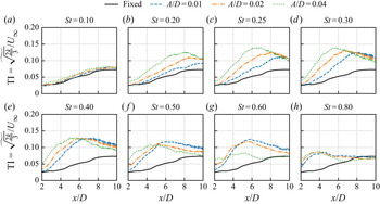
Figure 21 compares the turbulence intensity averaged in the spanwise direction over one rotor diameter on the hub-height plane. Except for the case with the lowest frequency ( $St=0.10$) of turbine motion, all cases show significant increases of TI when compared with the fixed one (black line). For cases with the same Strouhal number in the frequency range
 $0.20 \le St \le 0.60$, it is found that increasing the amplitude of turbine motion increases the TI for a certain range of turbine downstream distances, which becomes shorter for large motion frequencies. At further downstream locations beyond this range, the TI values due to different motion amplitudes are similar to each other for the case with
 $St=0.25$, while the TI values are larger for smaller motion amplitude in cases with
 $0.3 \le St \le 0.6$. For the case with the highest frequency (
 $St=0.80$), the TI values from the cases with different amplitudes are approximately the same as each other, being higher than the fixed turbine case for
 $x/D<8$ and approximately the same as the fixed turbine at further downstream locations. For all cases, the TI first increases to a peak and then decreases. The value of the peak and its location are dependent on both the frequency and the amplitude of the turbine motion. When comparing cases with the same motion frequency, it is found that the peak location moves upstream with increasing motion amplitude for
 $0.2 \le St \le 0.6$. The maximum value of TI increases with turbine motion amplitude for cases with low frequencies (
 $0.2\le St \le 0.40$), while it decreases for
 $St =0.5, 0.6$.
Turbulence intensity (averaged in space over one rotor width) for cases with different turbine oscillation frequencies and motion amplitudes.

3.3. Effects of inflow turbulence and shear
The above analyses have been focused on cases under uniform inflow. In this subsection, how inflows with turbulence or shear affect the onset of wake meandering is assessed for the oscillating turbine with  $St=0.25$ and
 $A/D=0.04$, in order to examine the existence of wake meandering induced by turbine side-to-side motion under more realistic wind conditions.
3.3.1. Inflow turbulence
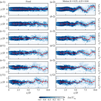
The effects of inflow turbulence on the onset of meandering induced by turbine side-to-side motion are examined in this subsection. As can be seen in figure 22, the wake of the fixed turbine is rather steady when the inflow turbulence is null or small, e.g. for cases with  $\sigma _u/U \le 3.8\,\%$. At these low turbulence levels, the effect of side-to-side motion on triggering the meandering motion can be distinguished visually. For inflows with higher turbulence intensity (
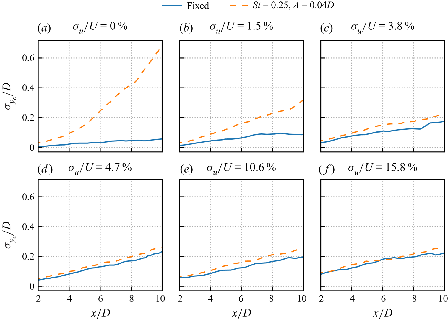
 $\sigma _u/U \ge 4.7\,\%$), the meandering patterns between the fixed and oscillating turbines are similar to each other, as seen in figure 22. In figure 23, the standard deviations of instantaneous wake positions are compared for different inflow turbulence intensities. It is observed that the meandering amplitudes are in general increased because of the turbine side-to-side motion. However, such increases become smaller for higher inflow turbulence intensities, and are negligible for the case with
 $\sigma _u/U = 15.8\,\%$.
Comparison of instantaneous velocity deficits behind a fixed turbine (in the first column) and an oscillating turbine (in the second column) for different inflow turbulence intensities  $\sigma _u/U$. Inflows are synchronized for figures in the same row; turbine side-to-side motion synchronized in phase for figures in the second column. Fitted wake centrelines are plotted with red dashed lines.

Standard deviation of instantaneous wake centre locations for cases with different inflow turbulence intensities  $\sigma _u/U$.

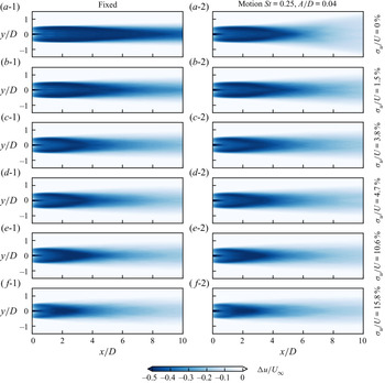
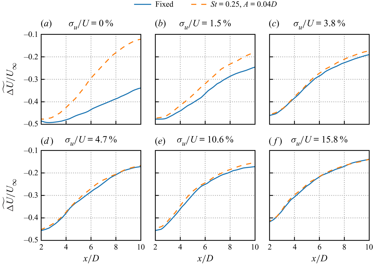
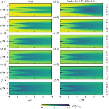
The time-averaged velocity deficits for cases with different inflow turbulence intensities are examined in figures 24 and 25. For the fixed turbine cases, increasing the inflow TI monotonically accelerates wake recovery. In contrast, the wake recovery is slowed down when the inflow turbulence intensity is increased from 0 % to 1.5 % for the oscillating turbine case. As shown in figure 25, the wake recovery enhancement due to the side-to-side motion of the turbine is observed only for cases with  $\sigma _u/U \le 3.8\,\%$, while it becomes negligible when
 $\sigma _u/U \ge 4.7\,\%$.
Comparison of time-averaged velocity deficits in the fixed frame of reference behind a fixed turbine (in the first column) and an oscillating turbine (in the second column) for different inflow turbulence intensities  $\sigma _u/U$.

Velocity deficit in the wake behind a fixed and an oscillating wind turbine averaged in time and in space (over the width of the turbine) for cases with different inflow turbulence intensities  $\sigma _u/U$.

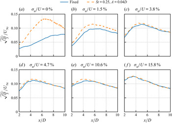
The wake turbulence is analysed in figures 26 and 27. From both figures, it is found that the effect of side-to-side motion on the wake turbulence also diminishes with increasing inflow turbulence intensities. By carefully analysing figure 27(a), one can find that the pure side-to-side motion induces TI of approximately 4 % in the near wake (at  $x=2D$). It is worth noting that this TI can be employed to indicate the energy of the perturbation induced by the turbine side-to-side motion. This energy level is found to be lower than that induced by the inflow turbulence for cases with
 $\sigma _u/U = 3.8\,\%$ (figure 27c), i.e. the inflow may violently destroy the harmonic perturbations induced by the turbine side-to-side motion, and hampers their development. This comparison could explain why the wake evolution is dominated by the inflow turbulence rather than the turbine side-to-side motion for cases with high inflow turbulence intensity.
Comparison of the turbulence intensity  $\sqrt {{{2k}/{3}}}/U_\infty$ in the fixed frame of reference behind a fixed turbine (in first column) and an oscillating turbine (in the second column) for inflow with different
 $\sigma _u/U$.

Turbulence intensity in the wake behind a fixed and an oscillating wind turbine averaged in time and in space (over the width of the turbine) for inflows with different  $\sigma _u/U$.

3.3.2. Wind shear effects
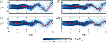
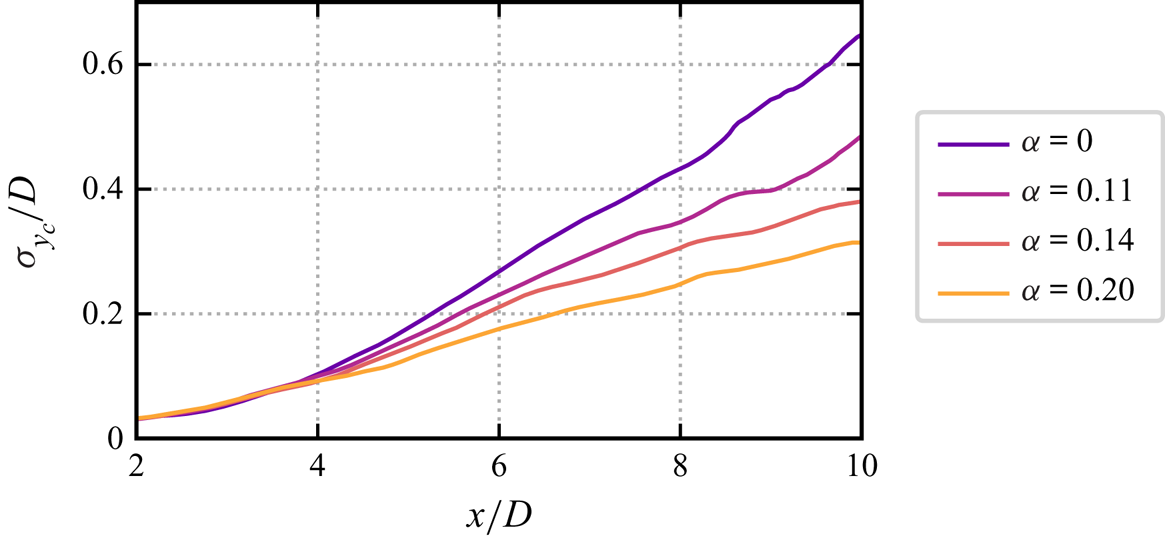
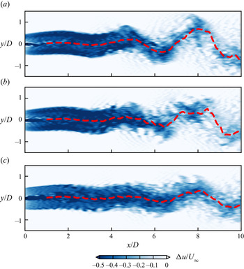
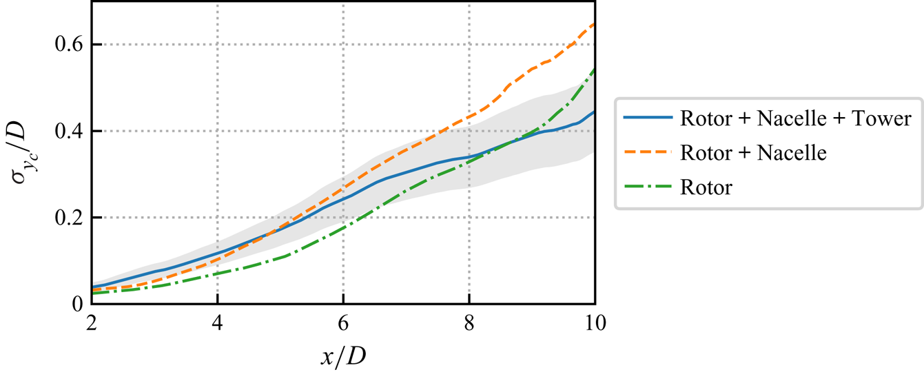
This subsection investigates the effects of vertical wind shear on the onset of wake meandering induced by turbine side-to-side motion. The vertical shear results in wind speed variation on the rotor's sweeping plane, and thus challenges the hypothesis of axisymmetric flow employed for local LSA. Results of LES are employed to verify how the wake meandering can be affected by including vertical wind shear. Figure 28 shows the instantaneous streamwise velocity deficit on the hub-height plane. As can be seen, similar wake meandering patterns are observed, although the axisymmetry is lost for cases with non-zero wind shear exponents. The quantitative comparison in figure 29 shows that the wake meandering amplitude, indicated by the standard deviation of the wake centre locations  $\sigma _{y_c}$, decreases with increasing wind shear exponent
 $\alpha$, suggesting an attenuation effect of the wind shear on the wake meandering. It is worth noting that the shear-generated turbulence will also be involved in the streamwise evolution of the wake. We argue that the vertical shear is the major factor for the different trends shown in figure 29, as the turbulence intensities resulting from the vertical shear are fairly small and approximately the same for the considered non-zero shear exponents (see details in § 2.3).
Instantaneous wake deficit behind the oscillating wind turbine for different wind shear exponents  $\alpha = 0$ (a),
 $\alpha = 0.11$ (b),
 $\alpha = 0.14$ (c),
 $\alpha = 0.20$ (d).

Standard deviation of the instantaneous wake centre location  $\sigma _{y_c}$ for cases with different inflow wind shear exponents.

4. Discussion
The most important finding from this work is that turbine side-to-side motion can be a novel origin for the onset of wake meandering. This finding is of particular importance for FOWTs because their compliant foundations are easily subject to motions induced by waves/winds. Platform motions at certain frequencies can be amplified in the far wake due to wake instability, and lead to wake meandering with amplitude comparable to the turbine rotor diameter. As revealed by the frequency analysis, the meandering motion is strongly related to that of the side-to-side motion and well preserved in the entire wake, being distinctively different from the meandering motion caused by inflow turbulence. The PDF of the instantaneous wake centre positions, which features two peaks, one at each extremity, being consistent with the PDF of the side-to-side FOWT motion, is significantly different from the normal distribution commonly observed for wake meandering in the literature. On the other hand, the mechanism of the wake meandering induced by turbine side-to-side motion is related to the mechanism discovered in the literature (Iungo et al. Reference Iungo, Viola, Camarri, Porté-Agel and Gallaire2013; Kang et al. Reference Kang, Yang and Sotiropoulos2014; Mao & Sørensen Reference Mao and Sørensen2018; Gupta & Wan Reference Gupta and Wan2019; Yang & Sotiropoulos Reference Yang and Sotiropoulos2019). These meandering mechanisms can be classified based on the role of turbine wake: (1) amplifier of disturbances (i.e. the shear layer instability mechanism); (2) passive scalar following the inflow (i.e. the large-eddy mechanism). When the wake acts as a passive scalar, the meandering frequency will be determined by the typical frequency of the inflow large-scale eddies, which may have a much broader spectrum. When it acts as an amplifier, the meandering mechanism can be considered as an intrinsic property of the wake, and the range of frequencies is similar to the vortex-shedding frequencies of a bluff body (Heisel et al. Reference Heisel, Hong and Guala2018; Yang & Sotiropoulos Reference Yang and Sotiropoulos2019). In the literature, such disturbances are from either the inflow (Mao & Sørensen Reference Mao and Sørensen2018; Gupta & Wan Reference Gupta and Wan2019) or the hub vortex (Iungo et al. Reference Iungo, Viola, Camarri, Porté-Agel and Gallaire2013; Kang et al. Reference Kang, Yang and Sotiropoulos2014). The results presented in this work show that disturbances caused by turbine side-to-side motion with frequencies falling into the same range can also trigger the onset of meandering. Simulations with different inflows show that the meandering induced by turbine side-to-side motion is influenced by and coupled with the inflow turbulence. When the inflow turbulence intensity is low ( ${\rm TI} \le 1.5\,\%$ for the present cases), the side-to-side motion mechanism dominates the evolution of wake meandering. For high turbulence intensity (e.g.
 ${\rm TI}=15.8\,\%$), on the other hand, the inflow turbulence mechanism suppresses the side-to-side motion mechanism. For intermediate inflow turbulence intensities, the two mechanisms are coupled with each other, which needs further systematic study. We want to emphasize that the onset of the meandering induced by turbine side-to-side motion does not need any inflow disturbances, while the meandering induced by inflow turbulence occurs only when the inflow turbulence intensity is high enough. Based on the above arguments, this work complements the existing wake meandering mechanism from both theoretical and practical points of view: (1) the disturbance introduced by turbine side-to-side motion is a new source for triggering the shear layer instability; (2) the wake meandering induced by turbine side-to-side motion should be considered at low inflow turbulence intensity, together with that induced by inflow turbulence at moderate and high inflow turbulence intensities.
Second, the considered ideal cases are related to real FOWT conditions. The target wind turbine in this study (NREL 5 MW reference wind turbine) is one of the most studied turbines for FOWT research. The frequencies and amplitudes considered in the present cases are feasible in realistic applications. The turbine motion amplitudes, being less than  $0.04D$, are within the design requirement for offshore wind turbines (Nejad et al. Reference Nejad, Bachynski and Moan2019). The frequencies resulting in the significant far wake meandering fall in the range
 $0.2 \le {St} \le 0.6$, although, being lower than the wave frequencies commonly encountered (corresponding to
 $St > 1.0$ for the present turbine design), they are within the range of the natural motion frequencies of the floating platform, indicating the importance of considering wake meandering induced by FOWT motion in the design of FOWT farms. For example, the well-studied reference offshore wind turbine platform, the DeepCwind semi-submersible platform (Robertson et al. Reference Robertson2014), has natural roll period about 26 s (
 $St \approx 0.4$), which will dominate the platform motion when second-order wave forces are considered (Mahfouz et al. Reference Mahfouz, Molins, Trubat, Hernández, Vigara, Pegalajar-Jurado, Bredmose and Salari2021). The present work shows that this design may trigger large-amplitude far wake meandering when the platform oscillates at its natural roll frequency under low ambient turbulence. On one hand, the induced wake meandering can help wake recovery. On the other hand, wake meandering at a frequency close to the platform's natural frequency may even trigger large motion of the platform of downstream turbines like a chain reaction, which may eventually propagate in the entire wind farm. This trade-off between benefit and risk must be considered carefully when designing the hydrodynamic properties of a platform.
Third, the present work demonstrates that local LSA can be employed to develop low-order models for predicting wake meandering caused by side-to-side motion of FOWTs. The comparison between the predictions from LSA and LES shows that local LSA can predict the least stable frequency and the amplification factor with a reasonable accuracy, especially when the imposed turbine motion is small (e.g.  $A/D = 0.01$). Although the amplification factors are overpredicted by LSA, especially for turbine motions with high amplitudes as a result of the nonlinear effect, the local LSA employed in this work can at least give an upper bound for the meandering motion in the far wake. Besides the nonlinearity effects, the inviscid fluid assumption may also lead to overpredictions of the amplification factor for LSA, which can be incorporated in future studies to further improve the accuracy of the present LSA, such as including the nonlinearity from using the complex Ginzburg–Landau equation (Gupta & Wan Reference Gupta and Wan2019), and adding the eddy viscosity to the linearized Navier–Stokes equations as shown by Rukes et al. for a turbulent jet flow (Rukes, Paschereit & Oberleithner Reference Rukes, Paschereit and Oberleithner2016), for which the eddy viscosity could be obtained using a data-driven approach (Zhang, Michelén-Ströfer & Xiao Reference Zhang, Michelén-Ströfer and Xiao2020).
5. Summary and conclusions
The effects of side-to-side harmonic oscillations of a floating offshore wind turbine on the wake evolution are investigated using large-eddy simulations of the NREL 5 MW offshore wind turbine parametrized with the actuator surface model. In the simulated cases, side-to-side motions of the turbine with different frequencies and amplitudes are prescribed. The simulation results show that side-to-side motions with frequencies in the range  $0.2 \le St \le 0.6$, which overlap with the wake meandering frequencies due to the shear layer instability, can trigger far wake meandering (see figure 15). To the best of the authors’ knowledge, this work for the first time shows that turbine side-to-side motion of very small amplitude (which can be just 1 % of rotor diameter) can trigger wake meandering of amplitude of the order of rotor diameter. It suggests that turbine side-to-side motion is a novel origin for triggering the onset of the shear layer instability mechanism. However, the sinusoidal shape wake meandering patterns observed in the simulated cases, with the meandering frequency and the PDF of instantaneous wake positions dominated by the side-to-side motion of FOWTs, are different from those induced by inflow turbulence (see figure 8).
The effects of inflow turbulence and vertical shear on the onset of meandering induced by turbine side-to-side motion are examined. The vertical shear is found to reduce the meandering amplitude in the hub-height plane (see figure 28). The effect of inflow turbulence, on the other hand, is more complex. It is found that the wake meandering induced by turbine side-to-side motion is suppressed by inflow large eddies once the inflow turbulence intensity is higher than 4.7 % for the considered motion amplitudes (see figures 22 and 23). However, the relative importance of inflow turbulence and FOWT motion will be analysed further by expanding the parameter space in future work.
Moreover, this work shows that such wake meandering induced by FOWT side-to-side motion can be predicted acceptably using local LSA. Using only the streamwise velocity component of the time-averaged wake behind a stationary turbine as the base flow, local LSA is able to predict the unstable frequency range with reasonable accuracy at negligible computational expense (see figure 14). In the meantime, the simulation results also show that local LSA slightly overpredicts the most unstable frequency and greatly overpredicts the amplification factors for high amplitudes of the side-to-side FOWT motion because of the nonlinear effect (see figure 17), which cannot be considered yet in the employed local LSA.
We emphasize that the most important finding from this work is that turbine side-to-side motion can be a novel origin for the onset of wake meandering when the inflow turbulence is low. From a practical point of view, turbine side-to-side motion has a twofold influence on downstream neighbours. On one hand, violent wake meandering in the far wake induces strong unsteady loads. On the other hand, the meandering enhances the mixing between the wake and the freestream, and consequently accelerates the recovery of the time-averaged velocity deficit, which benefits the overall power output of the wind farm. Moreover, analyses using the methodologies employed in this work, i.e. LES and LSA, can be integrated in the design stage of FOWT. The present work shows that the wake's unstable frequencies lie over a broad range and overlap with the floater's natural frequencies, thus this kind of wake meandering is highly probable with the present floater designs. Predicting the unstable frequency range of the wake as done in this work can provide an important criterion for the design of the floater's natural frequency no matter whether the wake meandering induced by the turbine side-to-side motion is considered helpful or harmful.
It is worth noting that the scenario considered in the present work is rather idealized (i.e. only simple harmonic side-by-side turbine motion is considered) to facilitate the analyses of the wake's essential features. In real-world applications, an FOWT is subject to complex motions of six degrees of freedom induced by both wave (Liu et al. Reference Liu, Xiao, Incecik and Wan2016) and wind in the ocean atmospheric boundary layer (Rockel et al. Reference Rockel, Camp, Schmidt, Peinke, Cal and Hölling2014; Wise & Bachynski Reference Wise and Bachynski2020). Investigations on other types of FOWT motion are underway, which will be presented in future work. These interactions between the wind, the FOWT and the waves, which can be solved using fully coupled two-phase CFD solvers (Li et al. Reference Li, Deng, Queutey, Bouscasse, Ducrozet, Gentaz, Le Touzé and Ferrant2019; Zhu, Goraya & Masud Reference Zhu, Goraya and Masud2019; Gatin et al. Reference Gatin, Liu, Vukčević and Jasak2020; Li et al. Reference Li, Bouscasse, Ducrozet, Gentaz, Le Touzé and Ferrant2021; Zhu & Masud Reference Zhu and Masud2021), are not considered, and will also be studied in a systematic way in future work.
Funding
This work was partially supported by the NSFC Basic Science Center Program for ‘Multiscale Problems in Nonlinear Mechanics’ (grant no. 11988102). This work was also supported by the National Natural Science Foundation of China (grant no. 12172360).
Declaration of interests
The authors report no conflict of interest.
Appendix A. Effect of rotor parametrization method
This appendix evaluates the predictive capability of the actuator disk (AD) model for the wake of an oscillating turbine by comparing the AD results with those from the actuator surface (AS) model. Two types of AD model with the same thrust are examined, the first with radially dependent force, and the second with uniformly distributed force. The AS model for the nacelle is employed for both AD models. In this work, the AS simulation is carried out first to obtain the time-averaged thrust and its radial distribution. The AD simulations are then carried out with the thrust obtained from the AS simulation.
Figures 30 and 31 compare the instantaneous wake and the standard deviation of the wake centre locations  $\sigma _{y_c}$ from the AD simulation with those from the AS simulation. As can be seen, using the uniformly loaded AD model results in significant underprediction of the wake meandering amplitude (about 50 % for
 $\sigma _{y_c}$ at
 $x=8D$ when compared with the AS prediction). Including the radial thrust distribution in the AD model can remarkably improve the AD predictions, reducing the maximum error to approximately 20 %. This improvement shows the importance of correctly modelling the radial force distribution for the AD model to predict the wake meandering of an oscillating turbine. Further studies may consider the wake rotation (Wu & Porté-Agel Reference Wu and Porté-Agel2011), i.e. to include the tangential forces on the non-uniform AD model, to check its effect on the wake meandering.
Instantaneous wake deficit behind an oscillating wind turbine simulated with different rotor parametrization approaches: (a) actuator surface method; (b) actuator disk method with radially dependent thrust equal to actuator surface method; (c) actuator disk method with uniform thrust distribution. The red dashed lines show the fitted instantaneous wake centre.

Standard deviation of the instantaneous wake centre location  $\sigma _{y_c}$ for cases with different rotor parametrization approaches. The grey shadow indicates the
 ${\pm }20\,\%$ limits around the AS result.

Appendix B. Effect of wind turbine tower and nacelle
This appendix evaluates the effect of a turbine's rotor, nacelle and tower on the wake meandering induced by turbine side-to-side motion. The nacelle and tower are modelled according to the NREL 5 MW wind turbine design (Jonkman et al. Reference Jonkman, Butterfield, Musial and Scott2009) using the actuator surface model (Yang & Sotiropoulos Reference Yang and Sotiropoulos2018). Three cases are considered: (1) with the nacelle, the tower and the rotor; (2) with the nacelle and rotor; (3) with the rotor only. In these simulations, the rotor is placed at  $z= 90$ m above the ground under uniform inflow to ensure that the height of the tower is correct. For simplification, the same side-to-side motion is imparted to the rotor, nacelle and tower together.
As can be seen from figure 32, all three cases show similar wake meandering patterns. However, it is found that the absence of a nacelle results in a jet in the wake centre, contrary to those cases with a nacelle. The quantitative comparison of the wake meandering amplitude (indicated by the standard deviation of wake centre position  $\sigma _{y_c}$) is shown in figure 33. It is seen that the predictions from the model with a nacelle and the model with both nacelle and tower are approximately the same at downstream locations near the turbine (
 $x/D<6$), and diverge at further downstream locations with higher meandering amplitude from the model with a nacelle. Moreover, it is seen that the meandering amplitude from the model with a nacelle (orange line) is higher than the one without (green line). This observation indicates that the nacelle wake can enhance the wake meandering, which is consistent with findings in the literature (Kang et al. Reference Kang, Yang and Sotiropoulos2014; Foti et al. Reference Foti, Yang, Shen and Sotiropoulos2019).
Instantaneous wake deficit behind an oscillating wind turbine at  $St = 0.25$ and
 $A=0.04D$. The red dashed lines show the fitted instantaneous wake centre. Panel (a) shows rotor
 $+$ nacelle
 $+$ tower, (b) shows rotor
 $+$ nacelle, and (c) shows rotor.

Standard deviation of the instantaneous wake centre location  $\sigma _{y_c}$ for cases with different model simplifications. The grey shadow indicates the
 ${\pm }20\,\%$ limits around the rotor
 $+$ nacelle
 $+$ tower result.