1. Introduction
In recent decades, major advances have been made in formalizing causation and causal inference (Pearl Reference Pearl2000; Spirtes, Glymour, and Scheines Reference Spirtes, Glymour and Scheines2000) and in using these formalisms to address traditional philosophical issues such as the nature of scientific explanation (Woodward Reference Woodward2003; Woodward and Hitchcock Reference Woodward and Hitchcock2003). At the heart of these formal theories lie causal models that involve elements such as causal graphs, probability distributions, Bayesian nets, and structural equations. Causal models are appreciated because they allow for inferring causal relations from observed probabilistic correlations and for predicting the effects of manipulations and interventions, and because they can be used for representing and explaining causal relationships in very general, formal terms.
Proponents of the causal modeling approach usually emphasize and exemplify the wide scope of this approach, for instance, by demonstrating its applicability to mechanistic explanations in biology and medicine (Casini et al. Reference Casini, Illari, Russo and Williamson2011; Clarke, Leuridan, and Williamson Reference Clarke, Leuridan and Williamson2014; Gebharter and Kaiser Reference Gebharter, Kaiser, Kaiser, Scholz, Plenge and Hüttemann2014). Similarly, Woodward’s (Reference Woodward2003) interventionist theory of causation and causal explanation, which makes extensive use of causal graphs, is supposed to be applicable to a wide range of causal relationships, including those in the biological realm (Woodward Reference Woodward2011, Reference Woodward2013).
In this article, I agree that causal modeling is a powerful approach to formally represent, explain, and discover causal relations. However, I also think that its scope should not be overestimated and that it is important to also recognize the limits of the causal modeling approach. This article explicates one of these limits: the explanation of spatially and structurally complex biological phenomena.Footnote 1 Based on the analysis of a case study from molecular biology, protein–DNA recognition, I show that the formal tools of causal graph theory are too limited to offer adequate causal explanations of the biological phenomena that essentially involve complex spatial and chemical-structural relations (e.g., complementarity of chemical structures, spatial fit between protein and DNA, DNA deformations).
Interestingly, Woodward has basically conceded this point, but he does not see this as a limitation of his causal modeling or interventionist approach to scientific explanation. Taking a relaxed stance, he argues that complex spatiotemporal information can just be added to the backbone of causal difference-making information and can be used to “organize” (Woodward Reference Woodward2011, 423) or “fine-tune” (Woodward Reference Woodward2013, 55) it. This article shows that things are not that easy. Some biological processes involve complex spatial and structural relations that are central to explaining these processes but that cannot be represented in causal graph models without rendering the model unexplanatory, unmanageable, or contradictory. To be clear: This is not a claim about biological practice, for instance, the claim that biologists wrongly use causal graphs to model certain phenomena. Rather, the purpose of this article is primarily philosophical. Given the increased popularity of causal modeling approaches, it is important to recognize not only their strengths but also their limits: which kinds of causal phenomena studied in biology cannot be explained by means of causal graphs, and why is this so?
I proceed as follows. Section 2 briefly reviews the core notions and assumptions made in the causal modeling literature. In section 3, I introduce my case study and carve out three kinds of information that any adequate explanatory model of protein–DNA recognition must include. Section 4 meets an important objection that challenges the overall project of this article and thereby clarifies the causal character of the explanation of protein–DNA recognition. I then construct a causal graph model of protein–DNA recognition (sec. 5), discuss different ways of including spatial-structural information in the model, and argue that each modeling strategy fails to yield an adequate explanation of the phenomenon (sec. 6).
2. Causal Modeling
Causal models can be grouped into two kinds: causal Bayesian networks and structural equation models. For the purposes of this article, I focus on causal Bayesian networks (also called causal graph models) and leave structural equations aside. Causal graph models combine mathematics and philosophy: the mathematical elements are directed acyclic graphs (DAGs) and probability theory; the philosophical elements are assumptions about the relationship between causation and probability (Spirtes et al. Reference Spirtes, Glymour and Scheines2000).
A DAG is an ordered pair G = <V, E>, where V is a set of variables and E is a set of directed edges (graphically represented by arrows). A variable can be binary, its values representing, for instance, the instantiation or noninstantiation of some property, or can have multiple values or even be continuous.
Besides the DAG, a causal model consists of a probability distribution P that assigns a real number 0 ≥ r ≥ 1 to every value combination of variables in V such that the sum of all assigned r equals 1. The pair of DAG G and probability distribution P over V is referred to as a Bayesian network if and only if G and P satisfy the Markov condition. A DAG becomes a causal graph as soon as its edges are interpreted causally: an edge leading from variable X1 to variable X2 is interpreted such that X1 is a direct cause of X2. When DAGs are interpreted causally, the Markov condition is assumed to be the correct connection between causal structure and probabilistic independence. This assumption is called the causal Markov condition (CMC): a DAG G and a probability distribution P over variable set V satisfy CMC iff every variable X in V is probabilistically independent of X’s nondescendants given X’s parents (i.e., INDEPPr(X, N-Des(X) | Pa(X))). CMC captures the intuition that conditioning on all common causes and on intermediate causes breaks down the probabilistic influence between two formerly correlated variables. Since causal models satisfy CMC, they allow for probabilistic prediction and manipulation.
3. Protein–DNA Recognition
Proteins that recognize and bind to specific DNA sequences are crucial to many biological processes. As transcription factors (TFs), they regulate gene transcription and thereby control processes such as cell differentiation. It is essential for the functioning of TFs that they recognize and bind selectively to only one or just a few specific DNA sequences out of the millions present in a genome. Understanding this specificity of protein–DNA recognition and binding is of considerable theoretical and practical importance.
Current biological research on protein–DNA recognition and binding is multifaceted. Among the different aspects that researchers study are the following:Footnote 2
1. Binding Sites Detection: Where in the genome are protein-binding sites located? Which DNA sequence does a particular TF bind? (See, e.g., Cai and Huang Reference Cai and Huang2012.)
2. Affinity/Specificity Measurements: How do the binding affinities of a TF vary for different sequences? How is the specificity of a TF measured? (See, e.g., Stormo and Zhao Reference Stormo and Zhao2010.)
3. Structure Determination: What is the structure of a protein–DNA complex? Which structural motifs do TFs use to bind to the DNA? (See, e.g., Harrison Reference Harrison1991.)
4. Recognition Mechanism Identification: How does a TF recognize its specific binding site? What are the mechanisms by which a TF reads out the DNA? (See e.g., Strauch Reference Strauch2001; Rohs et al. Reference Rohs, Jin, West, Joshi, Honig and Mann2010.)
In this article, I focus on the fourth set of questions and examine whether causal graph theory is an adequate tool for modeling mechanisms of protein–DNA recognition, without claiming that there must be a single model that captures all the different aspects of protein–DNA recognition and binding that are investigated in biological practice. To assess whether causal graph theory can be applied to mechanisms of protein–DNA recognition, I will first examine how biologists model and mechanistically explain how a TF recognizes its specific binding site. The aim of analyzing explanatory practice in biology is to reveal the kinds of information that are relevant to explaining this phenomenon and that thus must be included in any explanatory model of how protein–DNA recognition works.Footnote 3
Understanding the mechanisms of protein–DNA recognition has a long history. Initially, X-ray crystallography was used to uncover the structure of protein–DNA complexes (e.g., Pavletich and Pabo Reference Pavletich and Pabo1991). Crystallographic studies revealed that the surface of the DNA—in particular, its major groove—presents a distinctive pattern of hydrogen bond donors and acceptors and hydrophobic patches and that this pattern is recognized by a complementary set of donors and acceptors presented by the amino acid side chains of a TF. In other words, the TF recognizes the unique chemical signatures of the DNA bases of its binding site because its amino acids form a set of hydrogen bonds and hydrophobic contacts with the DNA bases. The specificity is conveyed not only through the number and kind of bonds formed but also through the uniqueness of the bonding geometry. These mechanisms of protein–DNA recognition are now commonly referred to as direct readout or “base readout” (Rohs et al. Reference Rohs, Jin, West, Joshi, Honig and Mann2010, 233).
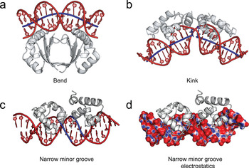
It was soon realized that the story is more complex than this because there is no one-to-one correspondence between DNA and protein sequences. For most TFs, the direct readout of base pairs through hydrogen bonds is thus not sufficient to explain their specificity. TFs recognize not only the chemical structure but also the shape of their DNA binding site. Depending on its sequence, DNA conformation can deviate from idealized B-DNA in various ways, each of which can be recognized by certain TFs. One of these ways is for the overall cylindrical shape of the DNA double helix to be deformed. For example, the DNA can be gradually bent, which can position elements of the DNA backbone such that these otherwise nonspecific contacts can become highly specific (fig. 1a). Another of these ways is for the geometry of the DNA to vary locally, for example, for the minor groove to be narrowed or the DNA to possess a kink. Minor groove narrowing typically enhances negative electrostatic potential, which then can be read by TFs (figs. 1c and 1d). Local kinks promote DNA conformations that optimize protein–DNA and protein–protein contacts (fig. 1b). Recognition mechanisms such as these are called indirect readout or “shape readout” (Rohs et al. Reference Rohs, Jin, West, Joshi, Honig and Mann2010, 233).
Examples of shape readout mechanisms (Rohs et al. Reference Rohs, Jin, West, Joshi, Honig and Mann2010, fig. 2).

In sum, biologists explain how a particular TF recognizes its specific binding site by describing the direct and indirect readout mechanisms that the TF combines to achieve the specificity required for its correct functioning. This explanation not only involves specifying the linear sequences of DNA and TF binding sites and revealing their complementarity by identifying the contacts that are made between bases and amino acids; it also requires describing their bonding geometry and how DNA and TF spatially fit, how the conformation of the DNA deviates from idealized B-DNA, and how this deviation facilitates further protein–DNA contacts.
I conclude that three kinds of information are relevant to explaining how protein–DNA recognition works:
1. binding information about the kinds of bonds that are formed between amino acid residues and DNA base pairs (direct contacts) and about the parts of the DNA and the TF that indirectly interact with each other (indirect contacts);
2. chemical-structural information about the primary sequences of DNA and TF binding sites and about the complementarity of their chemical structures;
3. spatial information about the conformations of DNA and the TF and why they spatially fit, and about how the DNA shape contributes to recognition.
Information of all three kinds is essential to explaining any mechanism of protein–DNA recognition because all three factors—causal interactions, chemical structural relations, and spatial relations—are crucial to the working of these mechanisms. Understanding how a TF recognizes a specific DNA sequence (out of the millions present in the genome) requires knowing how the TF reads out the chemical structure of the DNA binding site, how the two molecules spatially fit together, and how the structural complementarity and spatial fit enable specific bonds to be formed. Hence, any explanatory model of protein–DNA recognition is adequate only if it includes all three kinds of information.
4. Just a Matter of Noncausal Explanation?
Before I start modeling the phenomenon of protein–DNA recognition by means of causal graphs, this section addresses a possible objection and thereby further clarifies the main claim of the article. One might object that I am accusing causal graph theory of not being able to do something that it was never intended to do, namely, represent noncausal explanations such as the explanation of how a particular protein recognizes its specific binding site. My response to this objection is threefold.
First, I do not agree that explanations of protein–DNA recognition are noncausal. Describing the recognition mechanisms that are at work in a particular case includes also specifying which functional groups of the DNA and the protein interact with each other to form certain kinds of bonds. The formation of chemical bonds, however, clearly is a causal process, which is why the explanation of protein–DNA recognition will be, at least partially, also causal.
Second, granted that binding information is information about causal relations, an opponent might still insist that the rest of the explanation represents noncausal relations, namely, chemical structures, shapes, and spatial relations. Since causal graph theory was designed to represent causal dependencies only, as the opponent claims, why should one care about the news that these noncausal relations cannot be adequately represented in a causal graph model? One possible response to this objection is to point to the fact that philosophers actually are interested in this question. Whether noncausal relations such as supervenience or constitution relations can be represented in causal graph models or can be dealt with in an interventionist framework is controversially discussed (e.g., Casini et al. Reference Casini, Illari, Russo and Williamson2011; Gebharter and Kaiser Reference Gebharter, Kaiser, Kaiser, Scholz, Plenge and Hüttemann2014; Baumgartner and Gebharter Reference Baumgartner and Gebharter2015; Woodward Reference Woodward2015). Thus, why not extend this discussion to other kinds of noncausal relations that play a central role in biological mechanisms?
Third, another, stronger response is to challenge the assumption that chemical-structural and spatial information is noncausal. According to many theories of causation, the shapes of DNA and the TF and the complementarity of their chemical structures turn out to be causes of the TF binding to DNA. In counterfactual terms, the complementarity of the chemical structures of DNA and the TF is a cause of the binding because if the chemical structures were not complementary, DNA and the TF would not bind. In an interventionist framework, for example, the bending of the DNA is a cause of the binding of a particular TF to the DNA because there is an ideal intervention such that if I intervene in the shape of the DNA and remove its bending, I will prevent the binding. Likewise, the three-dimensional conformation of the TF typically makes a difference to the binding and, thus, is a cause of it.Footnote 4 But if much of the chemical-structural and spatial information describes causes, then the question of this article seems to be even more pressing: Is there a way to include this causal information in a causal graph model? Can causal graph theory be used to model and explain spatially and structurally complex biological phenomena such as protein–DNA recognition, or does it reach its limits?
5. How to Model Protein–DNA Recognition by Causal Graphs
How can we construct a formal causal model of the mechanisms by which a TF recognizes its specific DNA binding site? What happens before the recognition is that the TF diffuses into the nucleus, establishes some nonspecific electrostatic interactions with the DNA backbone, which allows it to slide along the DNA (Strauch Reference Strauch2001), and finally encounters the DNA binding site in proper orientation. If recognition then occurs, it results in the binding of the TF to the DNA.
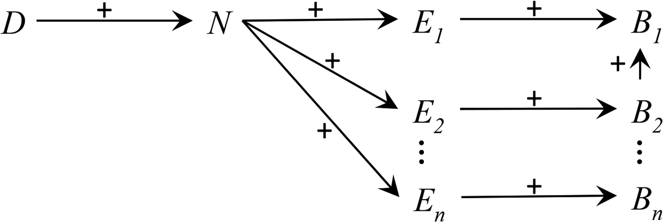
This causal chain of events (diffusion → nonspecific interactions → encountering → binding) is useful in understanding the causal context of the recognition process, but it does not explain how recognition itself occurs and how it ensures the specificity of the binding. As I pointed out in section 3, the latter requires, for instance, specifying which functional groups of the TF and the DNA encounter each other and which kinds of chemical bonds are formed. This binding information can be captured in a causal graph model not by introducing single variables for the encountering (E) and binding (B) of the TF and DNA, but rather by introducing fine-grained variables that represent subevents, such as the encountering of a certain region of the protein with a certain region of the DNA (E1, E2, … , En) and the formation of a certain kind of bond between a functional group of the protein and another of the DNA (B1, B2, … , Bn). The resulting causal graph model M1 is depicted in figure 2.
Causal graph model M1 for protein–DNA recognition.

In its simplest version, the variables in M1 are binary variables, representing events such as “TF diffuses into nucleus” (D), “nonspecific electrostatic interactions between TF and DNA backbone” (N), “a certain region of TF encounters a certain region of DNA binding site” (En), and “formation of two hydrogen bonds between amine-residue of lysine25 and the carbonyl- and pyridyl-group of DNA base guanine26” (B2). As binary variables, each of them can take one of the two values “taking place” and “not taking place.” Alternatively, they might be interpreted as quantitative variables. D and N would then stand for the number or concentration of particular TFs diffusing into the nucleus and nonspecifically interacting with the DNA backbone; E1, E2, … , En and B1, B2, … , Bn would stand for the number of encounterings and bond formations of the respective kinds. The arrows between the variables represent D being a direct cause of N, which is a direct cause of E1, E2, … , En, which are direct causes of B1, B2, … , Bn. The “+” stands for a positive causal influence: raising the probability that N takes a high value raises the probability that, for example, E3 takes a high value. Since the binding of an amino acid residue to a nucleotide base may raise the probability that another bond is established, the causal graph model also contains arrows between the B variables (e.g., the arrow between B1 and B2).
6. Where the Limits of Causal Graph Models Lie
The causal graph model M1 succeeds in representing binding information. Explaining how a TF recognizes a specific DNA sequence out of the millions present in a genome, however, not only requires specifying the chemical bonds that are formed but also requires elucidating the shapes of the TF and DNA, how they spatially fit, and how DNA conformation enables certain other interactions to occur (spatial information) and revealing the complementarity of the chemical structures of the TF and DNA (chemical-structural information). The latter two kinds of information, however, are missing in M1.
The causal modelers might agree with me at this point and concede the inadequacy of M1. But they might insist that it is possible to render M1 adequate by including the missing explanatorily relevant spatial and chemical-structural information. I see two major modeling strategies one could pursue. In what follows, I successively explain them and show why both fail to yield adequate explanations of protein–DNA recognition.Footnote 5
One option is to include the missing spatial and chemical-structural information in the characterization of the variables E1, E2, … , En and B1, B2, … , Bn. For instance, one could not only characterize B12 as “formation of two hydrogen bonds between amine-residue of lysine25 and the carbonyl- and pyridyl-group of DNA base guanine26” but also add “where the lysine25 residue is covalently bound to serine17 residue and leucine39 residue, forms a salt bridge to arginine9 residue, has a close distance to DNA bases cytosine28 and guanine42, etc.”
This strategy encounters three problems. First, storing complex spatial and structural information in the characterization of the variables renders M1 unmanageable because the measurement of the values of the variables becomes very complicated or even unfeasible in practice. This is a problem for causal models of this phenomenon in general, not a problem that pertains to explanation in particular. Second, the strategy results in a causal model in which the spatial and structural information is highly fragmented because information about the shapes of the TF and DNA, their spatial orientation to each other, the effect of DNA conformation on interactions between the TF and DNA, the chemical structures of the TF and DNA, and their complementarity is distributed over the variables E1, E2, … , En and B1, B2, … , Bn. This fragmentation is devastating to the explanatory power of the causal model since the resulting model fails to elucidate how spatial and chemical-structural relations contribute to the specificity of the recognition process (e.g., that TF and DNA spatially fit together and that DNA deformation enables specific interactions between the two macromolecules). Third, the modeling strategy gives rise to a causal model in which a great deal of the explanatorily relevant information is contained in the characterization of the variables, and not in the causal graphs that represent causal dependency relations. This suggests that the causal graphs are less informative and bear less explanatory weight than the characterization of the variables. But this seems to conflict with the typical way of conceiving causal graph models and reinforces the impression that one tries to add something that does not really fit.
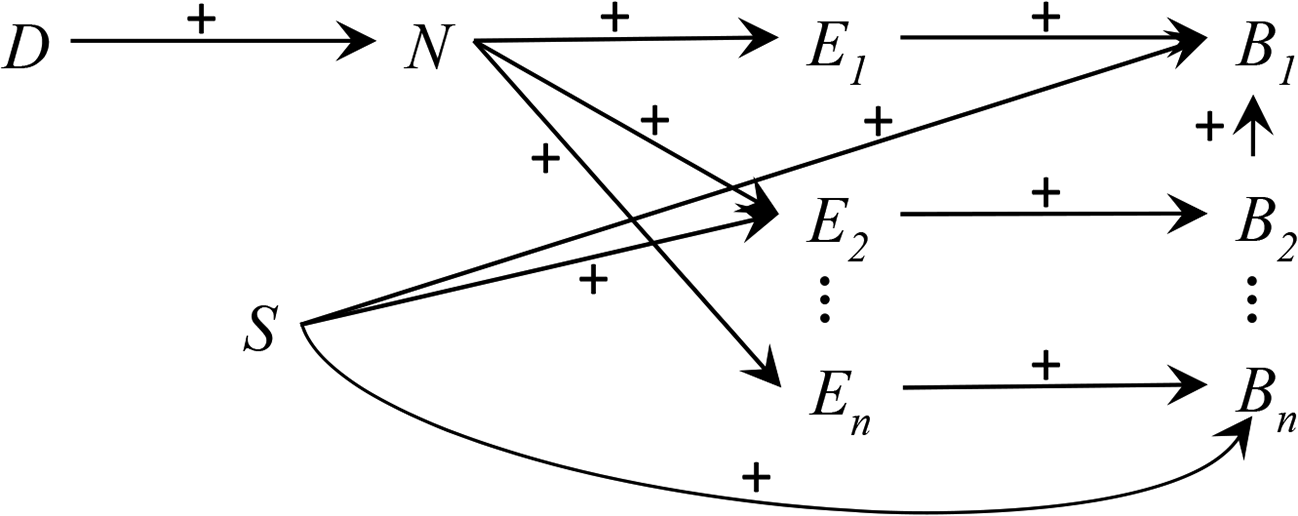
A second option is to add to the causal model one or more variables that are supposed to represent the spatial and chemical-structural information. One could, for instance, add the variable S that stands for the TF and DNA having certain conformations and chemical structures, the TF being oriented toward the DNA such that certain amino acid residues encounter certain DNA bases, the sequences of the TF and DNA being complementary. The resulting causal model M2 is depicted in figure 3.
Causal graph model M2 for protein–DNA recognition.

M2 accounts for the fact that whether or not a certain amino acid residue of the TF forms bonds to a certain DNA base depends not only on whether a particular TF region encounters the DNA binding site but also on whether the TF and DNA shapes enable the encountering in the first place (which is captured in fig. 3 by the arrow from S to E2), whether TF and DNA structures are complementary, and whether DNA deformation affects the binding (represented in fig. 3 by the arrows from S to B1 and Bn).
Despite these advantages, the revised causal model M2 is still not satisfactory. First, it has the feel of putting the missing relevant spatial and chemical-structural information in “by hand”: something that does not smoothly, automatically fit must be added under additional, atypical efforts. What reinforces this feeling is that all different spatial and chemical-structural information is represented by a single variable. It would be more adequate to add different variables (S1, S2, … , Sn) for the TF conformation, the DNA shape, the spatial orientation of the TF toward DNA, the amino acid sequence of the TF, the chemical structure of the DNA binding site, and the complementarity of the TF and the DNA structures. These different variables could also be quantitative variables that represent, for instance, relative distances among sets of TF molecules and sets of DNA molecules. But this modeling strategy encounters the problem that the variables are no longer conceptually independent of each other, which violates a central requirement of causal graph theory. For example, because a specific TF conformation (S3) requires a specific amino acid sequence (S5), a change in the value of S5 will simultaneously change the value of S3. Likewise, to say that TF and DNA binding sites are complementary (S2) is to say that certain kinds of chemical bonds can be formed (B1, B2, … , Bn), which is why S2 and B1, B2, … , Bn will be conceptually dependent. Finally, even if we could add different variables for each element of spatial and chemical-structural information, the characterization of S1, S2, … , Sn would remain very complex. This is due to the complexity of the shapes and spatial relations and to the large number of functional groups involved in the binding (see Rohs et al. Reference Rohs, Jin, West, Joshi, Honig and Mann2010). The second modeling strategy thus encounters the same objections as the first: storing complex information in the characterization of the variables renders the causal model unmanageable and contradicts the basic assumption of causal graph theory that directed graphs that represent causal dependency relations are central elements of causal models and thus neither are less informative nor bear less explanatory weight than the variables themselves.
To conclude, even if it might be in principle or technically possible to include information about complex spatial relations and chemical structures in a causal graph model, this can only be done at the expense of the adequacy of the causal model as it renders the causal model nonexplanatory (because the information gets highly fragmented) and unmanageable and entails inconsistencies with basic assumptions of causal graph theory (namely, that variables must be conceptually independent and that causal dependency relations are central). Hence, the causal graph approach reaches its limits when it comes to explaining spatially and structurally complex biological phenomena.
7. Conclusions
I agree that causal modeling is central to scientific practice and that formal theories of causal modeling and explanation, such as causal graph theory, are powerful. However, I think that their significance is not universal and that it is important to also notice the limits of causal graph theory. In this article, I have used an example from molecular biology to reveal one of these limitations: causal graph models fail to provide causal explanations of biological processes that involve complex spatial and chemical-structural relations.
My analysis of different modeling strategies has also shown why causal graph theory reaches its limits when trying to model cases such as protein–DNA recognition. One major obstacle is the huge extent and complexity of information about the parts of the involved molecules and their interactions that must be captured in the model. The other major obstacle is that there seems to be no way for a causal model to render intelligible the shapes of the two molecules, how they spatially fit together, and why this spatial fit enables certain other interactions to occur.