1 Introduction
When a liquid is forced to rapidly wet or dewet a solid surface, the capillary force fails to compete with the viscous drag, leading to the entrainment of gas or liquid on the solid, typically in the form of liquid films, droplets and gas bubbles (Snoeijer & Andreotti Reference Snoeijer and Andreotti2013). This dynamical wetting transition between wet and dry surfaces is encountered in a variety of natural and technological contexts, such as sliding drops (Podgorski, Flesselles & Limat Reference Podgorski, Flesselles and Limat2001), solid–liquid impact (Xu, Zhang & Nagel Reference Xu, Zhang and Nagel2005; Duez et al. Reference Duez, Ybert, Clanet and Bocquet2007) and coating (Weinstein & Ruschak Reference Weinstein and Ruschak2004). It is also of fundamental importance for clarifying various models of a moving contact line, whose underlying mechanisms remain under debate (Blake Reference Blake2006).
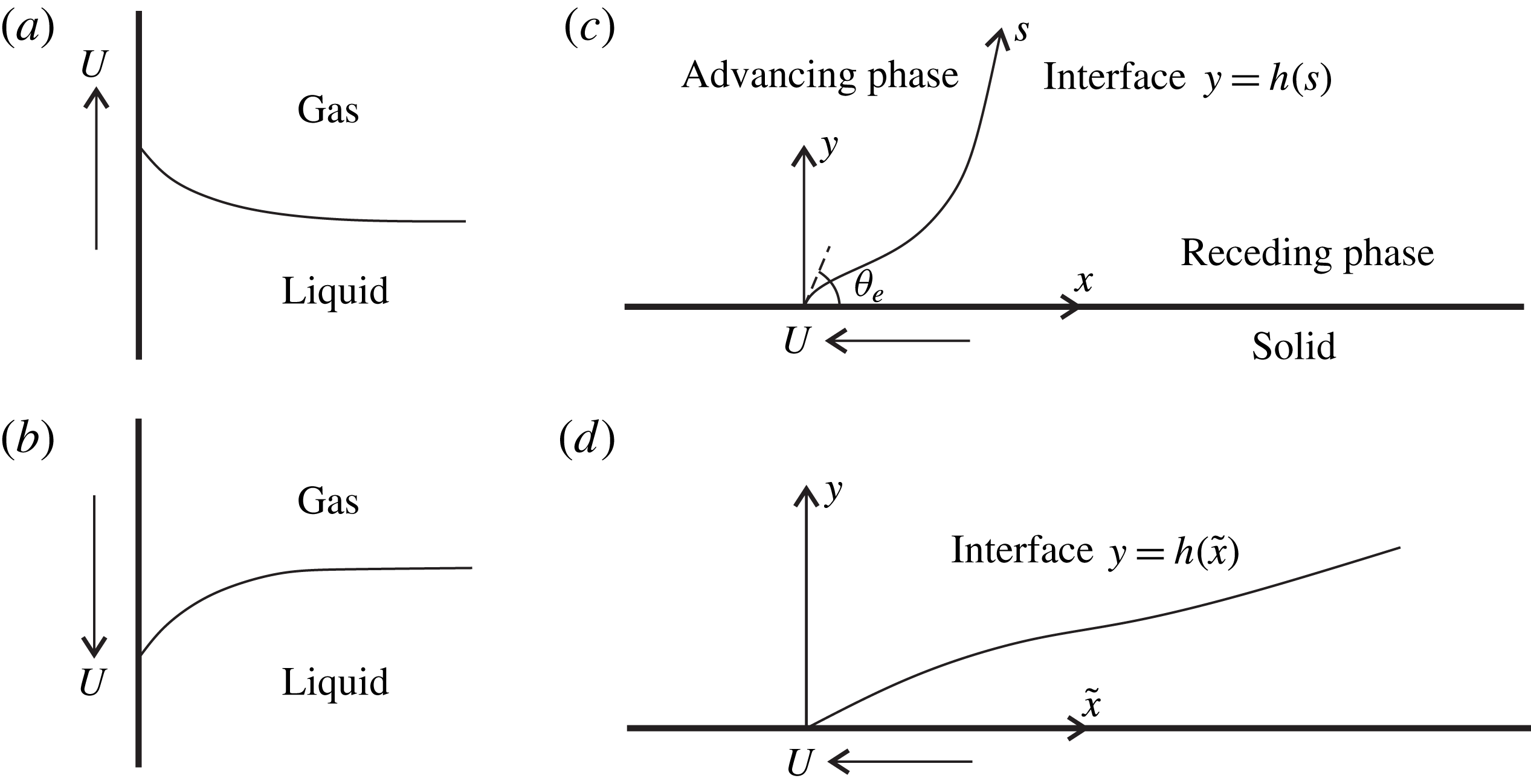
A representative set-up to investigate dynamical wetting transition is dip coating, in which a solid plate is withdrawn from or plunged into a liquid, as sketched in figure 1(a,b). In either configuration, the receding phase, either liquid or gas, will be entrained when the plate speed exceeds a threshold (Blake & Ruschak Reference Blake and Ruschak1979; Snoeijer et al. Reference Snoeijer, Delon, Fermigier and Andreotti2006; Benkreira & Ikin Reference Benkreira and Ikin2010; Marchand et al. Reference Marchand, Chan, Snoeijer and Andreotti2012), below which the gas–liquid interface behaves as a stationary meniscus. Of interest is how the critical speed depends on the properties of the fluids as well as their interactions with the plate.
The case of plate withdrawal, corresponding to receding contact lines, has been well understood in the framework of hydrodynamic theory, especially when the solid is hydrophilic and characterized by a small contact angle, usually measured in the liquid phase, such that classical lubrication theory (Oron, Davis & Bankoff Reference Oron, Davis and Bankoff1997) can be employed. It is the balance of capillarity, viscous force and gravity in the liquid phase that dominates the dynamics, while the gas can be neglected. The critical speed for liquid entrainment can be analytically predicted via an asymptotic matching procedure and is found to depend on both microscopic contact-line physics and macroscopic flow geometry (Eggers Reference Eggers2004, Reference Eggers2005; Chan, Snoeijer & Eggers Reference Chan, Snoeijer and Eggers2012). Moreover, it is demonstrated that the onset of liquid entrainment occurs when the corresponding apparent contact angle vanishes, i.e. the plate looks completely wettable on a macroscopic length scale. Beyond the transition, the entrained liquid film can exhibit a variety of interfacial morphologies due to the presence of the contact line (Snoeijer et al. Reference Snoeijer, Delon, Fermigier and Andreotti2006, Reference Snoeijer, Ziegler, Andreotti, Fermigier and Eggers2008; Galvagno et al. Reference Galvagno, Tseluiko, Lopez and Thiele2014; Gao et al. Reference Gao, Li, Feng, Ding and Lu2016), in addition to the traditional Landau–Levich–Derjaguin film (Landau & Levich Reference Landau and Levich1942; Derjaguin Reference Derjaguin1943).
Sketch of the dip-coating geometry. (a) Plate withdrawal. (b) Plate plunging. (c) Interfacial profile close to the contact line. (d) A coordinate transformation is introduced to reduce the slope angle of the interface.

The gas entrainment by advancing contact lines, on the other hand, is much more involved. Recent experiments have established the important role of the gas phase despite its small viscosity (Benkreira & Ikin Reference Benkreira and Ikin2010; Marchand et al. Reference Marchand, Chan, Snoeijer and Andreotti2012; Vandre, Carvalho & Kumar Reference Vandre, Carvalho and Kumar2012). This is due to the strong confinement of the gas by the plate and the liquid–gas interface close to the onset of transition. The thickness of the gas layer can even be comparable to the mean free path of gas molecules when the ambient pressure is sufficiently low (Sprittles Reference Sprittles2015, Reference Sprittles2017). In general, one has to numerically solve a two-phase Stokes flow (e.g. Vandre, Carvalho & Kumar Reference Vandre, Carvalho and Kumar2013), which is challenging due to the multi-scaled feature associated with the well-known contact-line singularity (Huh & Scriven Reference Huh and Scriven1971; Dussan & Davis Reference Dussan V and Davis1974). Alternatively, by considering the balance between capillarity, viscous force and contact-line friction, Ledesma-Aguilar, Hernández-Machado & Pagonabarraga (Reference Ledesma-Aguilar, Hernández-Machado and Pagonabarraga2013) presented a generic theory for the onset of liquid entrainment, without taking into account the macroscopic geometry. A more quantitative prediction was reported by Chan et al. (Reference Chan, Srivastava, Marchand, Andreotti, Biferale, Toschi and Snoeijer2013), who generalized the classical lubrication theory to two-fluid systems with small interfacial curvature and arbitrary interfacial slope, extending a prior work on a receding contact line with negligible gas (Snoeijer Reference Snoeijer2006). The critical speed of fluid entrainment in dip coating, obtained by numerically solving the generalized lubrication equation, seems promising for a wide range of wettability and viscosity ratio. However, an analytical prediction is still lacking, in contrast to the case of receding contact lines.
In this paper, we move forward by reporting an asymptotic solution of the onset of fluid entrainment in a generic two-fluid system. Accordingly, the entrainments of both liquid and gas act as two special limiting cases and are described in the same framework. The proposed procedure can also be easily extended to other geometries such as bubble/drop spreading and forced wetting in a capillary.
2 Theory
Consider the vertical translation of a solid plate with speed
 $U$
in two immiscible fluids, as sketched in figure 1. To study liquid and gas entrainment in a unified way, we employ a coordinate system with
 $x$
-axis directed towards the receding phase, and the fluid interface is described by
 $y=h(s)$
with
 $s$
the arclength (figure 1
c). We define the capillary number
 $Ca=\unicode[STIX]{x1D707}_{rec}U/\unicode[STIX]{x1D6FE}$
and the viscosity ratio
 $R=\unicode[STIX]{x1D707}_{adv}/\unicode[STIX]{x1D707}_{rec}$
, where
 $\unicode[STIX]{x1D6FE}$
is the surface tension, and
 $\unicode[STIX]{x1D707}_{rec}$
and
 $\unicode[STIX]{x1D707}_{adv}$
are the viscosity of the receding and advancing phase, respectively. Note that the gas is the receding phase for the case of plate plunging and
 $Ca$
is defined using gas viscosity; the capillary number based on liquid viscosity is simply
 $CaR$
. The contact angle
 $\unicode[STIX]{x1D703}_{e}$
is also measured in the receding phase. In the following, all lengths are scaled by the capillary length
 $\ell _{\unicode[STIX]{x1D6FE}}=\sqrt{\unicode[STIX]{x1D6FE}/(\unicode[STIX]{x0394}\unicode[STIX]{x1D70C}g)}$
, where
 $\unicode[STIX]{x0394}\unicode[STIX]{x1D70C}$
is the density difference of the two fluids and
 $g$
is the gravitational acceleration.
We focus on the situation where
 $\text{max}\{Ca,CaR\}\ll 1$
up to the entrainment. This means
 $\unicode[STIX]{x1D703}_{e}$
should not be too large, and
 $R$
remains finite for gas entrainment (Chan et al.
Reference Chan, Srivastava, Marchand, Andreotti, Biferale, Toschi and Snoeijer2013). For the case of gas entrainment into wetting liquids, the capillary number is typically
 $O(1)$
and is beyond the validity of the present theory. However, it will be shown that satisfactory results can still be obtained. To obtain the critical capillary number for fluid entrainment,
 $Ca_{c}$
, we explore the condition under which steady interfacial solutions exist. We develop an inner solution valid close to the contact line where viscous bending of the interface occurs (Voinov Reference Voinov1976; Cox Reference Cox1986), and an outer solution far away from it, and then match them following the procedure of Eggers (Reference Eggers2005). While the outer solution can be easily obtained for small capillary numbers, a crucial step here is to derive an analytical form of the inner solution.
2.1 Inner solution
The interface close to the contact line is determined by the balance between capillarity and viscous forces, and is governed by the generalized lubrication equations (Chan et al. Reference Chan, Srivastava, Marchand, Andreotti, Biferale, Toschi and Snoeijer2013)
 $$\begin{eqnarray}\frac{\text{d}\unicode[STIX]{x1D705}}{\text{d}s}=\frac{3Ca}{h(h+3\unicode[STIX]{x1D706})}f(\unicode[STIX]{x1D703};R),\quad \frac{\text{d}\unicode[STIX]{x1D703}}{\text{d}s}=\unicode[STIX]{x1D705},\quad \frac{\text{d}h}{\text{d}s}=\sin \unicode[STIX]{x1D703},\end{eqnarray}$$
with the boundary conditions at the contact line,
 $$\begin{eqnarray}s=0:\quad h=0,\quad \unicode[STIX]{x1D703}=\unicode[STIX]{x1D703}_{e}.\end{eqnarray}$$
Here,
 $\unicode[STIX]{x1D703}$
and
 $\unicode[STIX]{x1D705}$
denote the slope angle measured in the receding phase and the curvature of the interface, respectively;
 $\unicode[STIX]{x1D706}$
is an extremely small length to weaken the contact-line singularity, and reduces to the Navier slip length when
 $\unicode[STIX]{x1D703}\ll 1$
and
 $R=0$
. Note that this regularization still differs from that employing the Navier slip condition in general conditions, and is expected to induce a roughly logarithmic correction to the macroscopic solution. The function
 $f(\unicode[STIX]{x1D703};R)$
originates from the correction of the quasi-parallel flow employed in classical lubrication theory (Oron et al.
Reference Oron, Davis and Bankoff1997) by a wedge flow (Huh & Scriven Reference Huh and Scriven1971), and enables the application of (2.1) at large interface slopes. It can be written as
 $$\begin{eqnarray}f(\unicode[STIX]{x1D703};R)={\textstyle \frac{1}{3}}\,f_{Cox}(\unicode[STIX]{x1D703};R)\sin ^{2}\unicode[STIX]{x1D703},\end{eqnarray}$$
where
 $f_{Cox}(\unicode[STIX]{x1D703};R)$
is a complicated function first given by Cox (Reference Cox1986) (see appendix A).
We show that (2.1) can be simplified to the form of a classical lubrication equation governing the dynamics of a receding contact line, even though the contact line is advancing. To this end, we introduce a new coordinate
 $\tilde{x}=\tilde{x}(x)$
such that the interfacial profile is described by
 $y=h(\tilde{x})$
with a redefined slope
 $\tilde{\unicode[STIX]{x1D703}}\equiv \text{d}h/\text{d}\tilde{x}$
. While the form of the transformation will be determined later, we require that
 $\tilde{x}$
is positive and increases monotonically with the arclength
 $s$
or the interface height
 $h$
, and hence
 $\tilde{\unicode[STIX]{x1D703}}$
is non-negative. It can be proved that (see appendix B)
 $$\begin{eqnarray}\frac{\text{d}\unicode[STIX]{x1D705}}{\text{d}s}+\left(\ln \frac{\tilde{\unicode[STIX]{x1D703}}\tilde{\unicode[STIX]{x1D703}}^{\prime }}{\sin \unicode[STIX]{x1D703}}\right)^{\prime }\unicode[STIX]{x1D705}^{2}=\frac{\sin ^{2}\unicode[STIX]{x1D703}}{\tilde{\unicode[STIX]{x1D703}}^{2}\tilde{\unicode[STIX]{x1D703}}^{\prime }}\frac{\text{d}^{3}h}{\text{d}\tilde{x}^{3}},\end{eqnarray}$$
where a prime denotes the derivative with respect to
 $\unicode[STIX]{x1D703}$
. Note that (2.4) is independent of the specific form of the transformation and is a purely geometric relation, which connects the two forms of the curvature force,
 $\text{d}\unicode[STIX]{x1D705}/\text{d}s$
and
 $\text{d}^{3}h/\text{d}\tilde{x}^{3}$
, present in the generalized and classical lubrication equation, respectively. For the interface close to a moving contact line, we have
 $\unicode[STIX]{x1D705}\sim \max \{Cah^{-1},CaRh^{-1}\}$
and
 $\text{d}\unicode[STIX]{x1D705}/\text{d}s\sim \max \{Cah^{-2},CaRh^{-2}\}$
(Cox Reference Cox1986), and hence
 $\unicode[STIX]{x1D705}^{2}\ll |\text{d}\unicode[STIX]{x1D705}/\text{d}s|$
under the assumption of
 $\text{max}\{Ca,CaR\}\ll 1$
. Therefore, the second term in (2.4) can be neglected provided the coefficient of this term is regular. Substitution into (2.1) yields
 $$\begin{eqnarray}\frac{1}{\tilde{\unicode[STIX]{x1D703}}^{2}\tilde{\unicode[STIX]{x1D703}}^{\prime }}\frac{\text{d}^{3}h}{\text{d}\tilde{x}^{3}}=\frac{Ca}{h(h+3\unicode[STIX]{x1D706})}f_{Cox}(\unicode[STIX]{x1D703};R).\end{eqnarray}$$
By setting
 $\tilde{\unicode[STIX]{x1D703}}^{2}\tilde{\unicode[STIX]{x1D703}}^{\prime }=3/f_{Cox}(\unicode[STIX]{x1D703};R)$
, the new interface slope is determined as
 $$\begin{eqnarray}\tilde{\unicode[STIX]{x1D703}}(\unicode[STIX]{x1D703};R)=[9g(\unicode[STIX]{x1D703};R)]^{1/3}\equiv \left[9\int _{0}^{\unicode[STIX]{x1D703}}\frac{\text{d}\unicode[STIX]{x1D703}}{f_{Cox}(\unicode[STIX]{x1D703};R)}\right]^{1/3},\end{eqnarray}$$
which also provides a definition of
 $\tilde{x}$
through
 $$\begin{eqnarray}\tilde{x}=\int _{0}^{s}\frac{\sin \unicode[STIX]{x1D703}}{\tilde{\unicode[STIX]{x1D703}}}\,\text{d}s.\end{eqnarray}$$
Substitution of (2.6) into (2.5) yields
 $$\begin{eqnarray}\frac{\text{d}^{3}h}{\text{d}\tilde{x}^{3}}=\frac{3Ca}{h(h+3\unicode[STIX]{x1D706})}.\end{eqnarray}$$
The corresponding boundary conditions at the contact line can be easily obtained as
 $$\begin{eqnarray}\tilde{x}=0:\quad h=0,\quad \frac{\text{d}h}{\text{d}\tilde{x}}=\tilde{\unicode[STIX]{x1D703}}_{e}\equiv \tilde{\unicode[STIX]{x1D703}}(\unicode[STIX]{x1D703}_{e};R).\end{eqnarray}$$
Note that
 $g(\unicode[STIX]{x1D703};R)$
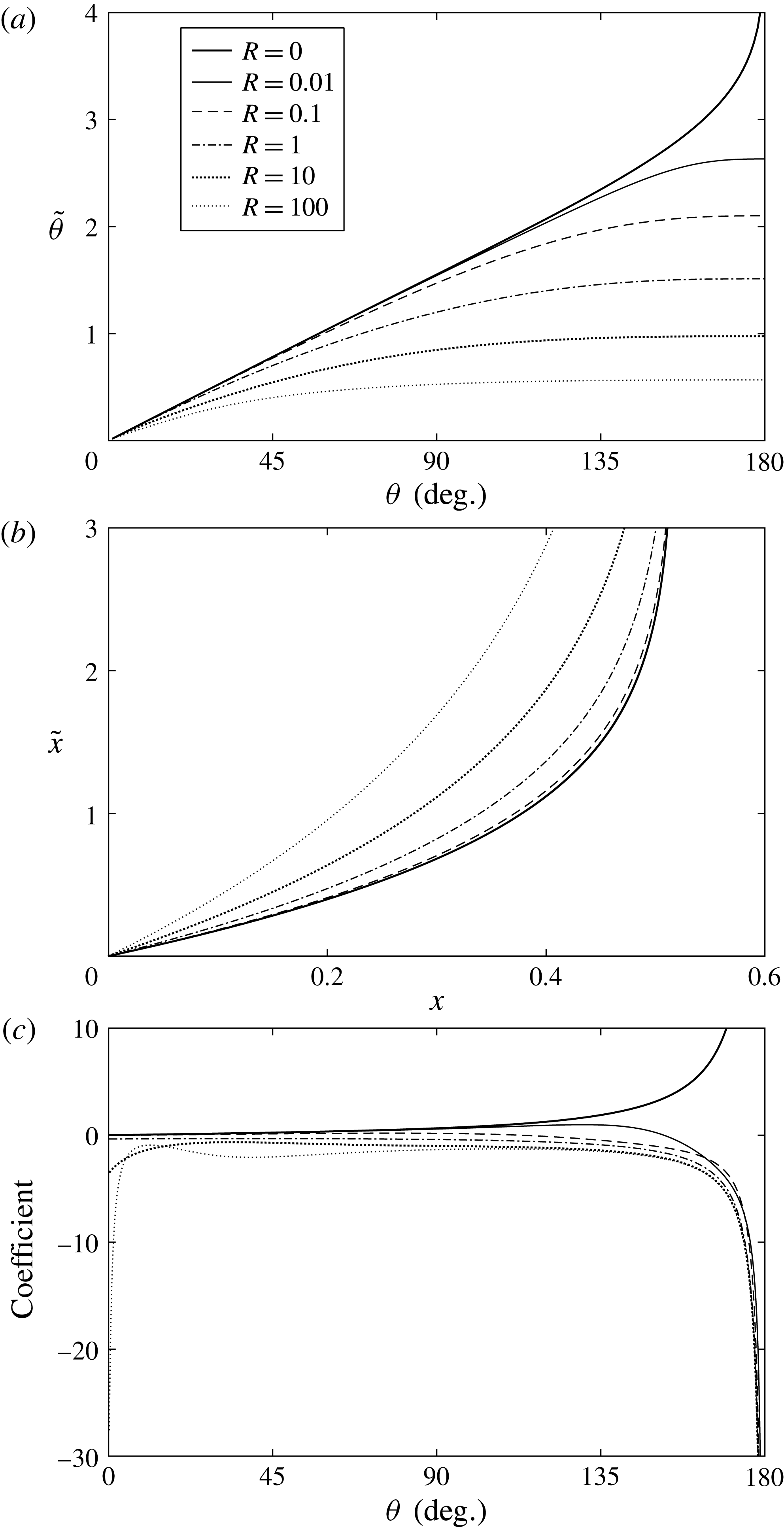
in (2.6) is exactly the well-known function reported by Cox (Reference Cox1986), and its behaviour has been discussed in detail therein. To depict the effect of the transformation, we plot the variation of
 $\tilde{\unicode[STIX]{x1D703}}(\unicode[STIX]{x1D703};R)$
with
 $\unicode[STIX]{x1D703}$
in figure 2(a), for representative values of
 $R$
. In figure 2(b), we show the relation between
 $\tilde{x}$
and
 $x$
for a stationary meniscus with
 $\unicode[STIX]{x1D703}_{e}=60^{\circ }$
. It can be seen that the interface angle is significantly reduced with the transformation; the interface is effectively stretched along the substrate, as also sketched in figure 1(d). For small slope angles, i.e.
 $\unicode[STIX]{x1D703}\ll 1$
, we have
 $\tilde{\unicode[STIX]{x1D703}}\approx \unicode[STIX]{x1D703}$
and
 $\tilde{x}\approx s\approx x$
; therefore, the proposed transformation plays a minor role on the interface. Furthermore, the coefficient of the second term in (2.4) is illustrated in figure 2(c). It is clear that the coefficient remains finite except when
 $\unicode[STIX]{x1D703}$
is close to
 $180^{\circ }$
, a region corresponding to a strong interface bending and beyond the scope of the present work. (Note that the coefficient is large but still finite at
 $\unicode[STIX]{x1D703}_{e}=0$
at large
 $R$
.) Therefore, the neglect of the second term at small capillary numbers is justified.
(a) Variation of
 $\tilde{\unicode[STIX]{x1D703}}$
as a function of
 $\unicode[STIX]{x1D703}$
. (b) Relation between
 $\tilde{x}$
and
 $x$
for the case of a stationary meniscus with
 $\unicode[STIX]{x1D703}_{e}=60^{\circ }$
. (c) Variation of the coefficient,
 $(\ln (\tilde{\unicode[STIX]{x1D703}}\tilde{\unicode[STIX]{x1D703}}^{\prime }/\sin \unicode[STIX]{x1D703}))^{\prime }$
, in (2.4) as a function of
 $\unicode[STIX]{x1D703}$
.

The simplified equation (2.8) has the form of classical lubrication equation, which governs the small-slope film flow characterized by a receding contact line and an effective interface slope
 $\tilde{\unicode[STIX]{x1D703}}_{e}$
at the substrate. It admits an analytical solution (Duffy & Wilson Reference Duffy and Wilson1997), which, for
 $\unicode[STIX]{x1D706}\ll \tilde{x}\ll 1$
, has the asymptotic form
 $$\begin{eqnarray}h(\tilde{x})=\frac{Ca^{1/3}\tilde{\unicode[STIX]{x1D703}}_{e}\exp [-\tilde{\unicode[STIX]{x1D703}}_{e}^{3}/(9Ca)]}{12^{2/3}\unicode[STIX]{x03C0}\unicode[STIX]{x1D706}\text{Ai}^{2}(t_{1})}\tilde{x}^{2}-\frac{(12Ca)^{1/3}\text{Ai}^{\prime }(t_{1})}{\text{Ai}(t_{1})}\tilde{x}+O(\unicode[STIX]{x1D706}),\end{eqnarray}$$
where
 $\text{Ai}(t_{1})$
is the Airy function of the first kind with the parameter
 $t_{1}$
to be determined by matching to the outer solution.
2.2 Outer solution
In the outer region where the flow can be neglected, the interface behaves as a stationary meniscus determined by the balance between gravity and surface tension. An analytical solution of the interface morphology is available (Landau & Lifshitz Reference Landau and Lifshitz1984; de Gennes, Brochard-Wyart & Quéré Reference de Gennes, Brochard-Wyart and Quéré2004). To match the inner solution, of relevance is the interface profile close to the contact line. For a meniscus with an apparent contact angle
 $\unicode[STIX]{x1D703}_{ap}$
, we introduce the apparent curvature of the interface at the contact line,
 $$\begin{eqnarray}\unicode[STIX]{x1D705}_{ap}=2\cos \left(\frac{\unicode[STIX]{x1D703}_{ap}}{2}+\frac{\unicode[STIX]{x03C0}}{4}\right).\end{eqnarray}$$
Then the interface profile close to the contact line can be written in terms of
 $\tilde{x}$
as (see appendix B)
 $$\begin{eqnarray}h(\tilde{x})=\tilde{\unicode[STIX]{x1D703}}_{ap}\tilde{x}+\frac{\unicode[STIX]{x1D705}_{ap}\tilde{\unicode[STIX]{x1D703}}_{ap}\tilde{\unicode[STIX]{x1D703}}_{ap}^{\prime }}{2\sin \unicode[STIX]{x1D703}_{ap}}\tilde{x}^{2}+O(\tilde{x}^{3}),\end{eqnarray}$$
for
 $\tilde{x}\ll 1$
, where
 $\tilde{\unicode[STIX]{x1D703}}_{ap}\equiv \tilde{\unicode[STIX]{x1D703}}(\unicode[STIX]{x1D703}_{ap};R)$
is the apparent slope of the meniscus at the contact line in the transformed frame.
2.3 Matching
Following Eggers (Reference Eggers2005), the matching of the inner and outer solutions, i.e. (2.10) and (2.12), leads to a system of equations for
 $\unicode[STIX]{x1D703}_{ap}$
and
 $t_{1}$
,
 $$\begin{eqnarray}\left.\begin{array}{@{}c@{}}\displaystyle \tilde{\unicode[STIX]{x1D703}}_{ap}=-\frac{(12Ca)^{1/3}\text{Ai}^{\prime }(t_{1})}{\text{Ai}(t_{1})},\\ \displaystyle \cos \left(\frac{\unicode[STIX]{x1D703}_{ap}}{2}+\frac{\unicode[STIX]{x03C0}}{4}\right)\frac{\tilde{\unicode[STIX]{x1D703}}_{ap}\tilde{\unicode[STIX]{x1D703}}_{ap}^{\prime }}{\sin \unicode[STIX]{x1D703}_{ap}}=\frac{Ca^{1/3}\tilde{\unicode[STIX]{x1D703}}_{e}\exp [-\tilde{\unicode[STIX]{x1D703}}_{e}^{3}/(9Ca)]}{12^{2/3}\unicode[STIX]{x03C0}\unicode[STIX]{x1D706}\text{Ai}^{2}(t_{1})},\end{array}\right\}\end{eqnarray}$$
provided that the other parameters are known. An analysis of these equations shows that the solutions with non-negative
 $\unicode[STIX]{x1D703}_{ap}$
can exist only when
 $Ca$
is less than a threshold,
 $Ca_{c}$
, which corresponds to
 $t_{1}=t_{max}\approx -1.0188$
, the largest maximum point of
 $\text{Ai}(t_{1})$
, and hence
 $\tilde{\unicode[STIX]{x1D703}}_{ap}=\unicode[STIX]{x1D703}_{ap}=0$
. Accordingly, we have
 $\tilde{\unicode[STIX]{x1D703}}_{ap}\tilde{\unicode[STIX]{x1D703}}_{ap}^{\prime }/\sin \unicode[STIX]{x1D703}_{ap}=1$
, and the second matching condition in (2.13) yields the critical capillary number
 $$\begin{eqnarray}Ca_{c}=\frac{\tilde{\unicode[STIX]{x1D703}}_{e}^{3}}{9}\left[\ln \left(\frac{Ca_{c}^{1/3}\tilde{\unicode[STIX]{x1D703}}_{e}}{2^{5/6}3^{2/3}\unicode[STIX]{x03C0}\unicode[STIX]{x1D706}\text{Ai}^{2}(t_{max})}\right)\right]^{-1},\end{eqnarray}$$
above which the interface would be unsteady, leading to the entrainment of the receding fluid. For convenience, the explicit form of
 $Ca_{c}$
can be written as
 $$\begin{eqnarray}Ca_{c}=\frac{\tilde{\unicode[STIX]{x1D703}}_{e}^{3}}{3W_{0}(\tilde{\unicode[STIX]{x1D703}}_{e}^{6}/(A\unicode[STIX]{x1D706})^{3})},\end{eqnarray}$$
where
 $A=2^{5/6}3\unicode[STIX]{x03C0}\text{Ai}^{2}(t_{max})\approx 4.818$
, and
 $W_{0}(t)$
is the Lambert
 $W$
function defined on the interval
 $t\geqslant -1/e$
(Corless et al.
Reference Corless, Gonnet, Hare, Jeffrey and Knuth1996). Note that the denominator can be approximated as
 $9L-3\ln L$
with
 $L=\ln (\tilde{\unicode[STIX]{x1D703}}_{e}^{2}/(A\unicode[STIX]{x1D706}))$
for
 $\unicode[STIX]{x1D706}\ll 1$
.
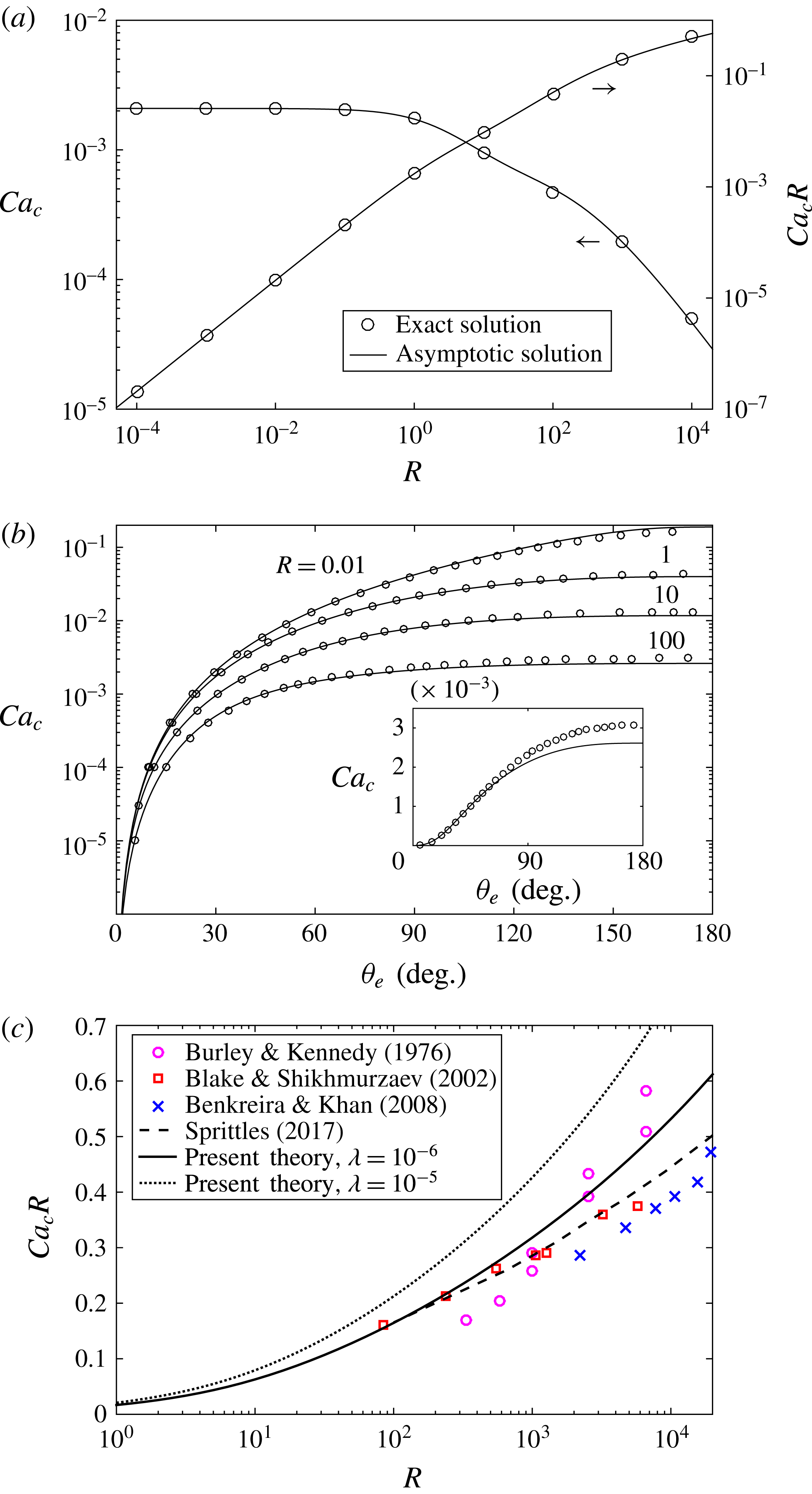
Variation of the critical capillary number with (a) the viscosity ratio
 $R$
at
 $\unicode[STIX]{x1D703}_{e}=30^{\circ }$
and (b) the contact angle
 $\unicode[STIX]{x1D703}_{e}$
for typical values of
 $R$
. The solid curves and circles represent the asymptotic solution, (2.14), and the exact solution obtained by numerically solving the generalized lubrication equation (Chan et al.
Reference Chan, Srivastava, Marchand, Andreotti, Biferale, Toschi and Snoeijer2013), respectively. The dimensionless slip length
 $\unicode[STIX]{x1D706}=10^{-5}$
. The inset in (b) reproduces the results of
 $R=100$
on linear scales. (c) Comparison of the present asymptotic solution at
 $\unicode[STIX]{x1D703}_{e}=90^{\circ }$
with experiments (Burley & Kennedy Reference Burley and Kennedy1976; Blake & Shikhmurzaev Reference Blake and Shikhmurzaev2002; Benkreira & Khan Reference Benkreira and Khan2008) and numerical simulations (Sprittles Reference Sprittles2017) for gas entrainment (
 $R\gg 1$
).

3 Results
The expression of
 $Ca_{c}$
, (2.14), has similar form to that of plate withdrawal with small contact angles (Chan et al.
Reference Chan, Snoeijer and Eggers2012), but with
 $\unicode[STIX]{x1D703}_{e}$
replaced by
 $\tilde{\unicode[STIX]{x1D703}}_{e}$
, which solely embodies the contributions of both viscosity ratio and large interface slope. For comparison, we have also calculated the critical capillary number by numerically solving the generalized lubrication equation via a shooting method, following Chan et al. (Reference Chan, Srivastava, Marchand, Andreotti, Biferale, Toschi and Snoeijer2013). As shown in figure 3(a), for
 $\unicode[STIX]{x1D703}_{e}=30^{\circ }$
, the asymptotic solution of
 $Ca_{c}$
agrees with the exact results very well over eight decades (
 $10^{-4}$
–
 $10^{4}$
) of
 $R$
, ranging from liquid to gas entrainment. The agreement is still satisfactory even though
 $Ca_{c}R$
is not so small (
 ${\sim}0.1$
) at large values of
 $R$
.
As a special case, the liquid entrainment in plate withdrawal, corresponding to receding contact lines, has been well studied based on classical lubrication theory (Chan et al.
Reference Chan, Snoeijer and Eggers2012). By setting
 $R=0$
, we have
 $\tilde{\unicode[STIX]{x1D703}}_{e}\approx \unicode[STIX]{x1D703}_{e}$
for
 $\unicode[STIX]{x1D703}_{e}\ll 1$
, and the formula of
 $Ca_{c}$
obtained by Chan et al. (Reference Chan, Snoeijer and Eggers2012) is recovered from (2.14). It is interesting to note that, when
 $R=0$
,
 $\tilde{\unicode[STIX]{x1D703}}_{e}$
can actually be well approximated by
 $\unicode[STIX]{x1D703}_{e}$
even for the latter up to
 $3\unicode[STIX]{x03C0}/4$
(Voinov Reference Voinov1976), suggesting the validity of classical lubrication theory at large contact angles. A further examination of figure 3(a) shows that
 $Ca_{c}$
is insensitive to
 $R$
provided
 $R\lesssim 0.1$
, and hence results of classical lubrication theory are also acceptable when the viscosity of the advancing phase is not negligible.
The more challenging case of gas entrainment corresponds to
 $R\gg 1$
. As shown in figure 3(a), the critical capillary numbers based on gas and liquid viscosity, i.e.
 $Ca_{c}$
and
 $Ca_{c}R$
, respectively, exhibit a significant dependence on
 $R$
, indicating the important role of both phases. It has been demonstrated by Cox (Reference Cox1986) that
 $g(\unicode[STIX]{x1D703};R)$
and
 $Ca_{c}$
depend linearly on
 $\ln (R)/R$
as
 $R\rightarrow \infty$
. Accordingly, since
 $\tilde{\unicode[STIX]{x1D703}}^{3}=9g(\unicode[STIX]{x1D703};R)$
, our results show a similar dependence, but with an additional logarithmic correction.
The effect of the contact angle
 $\unicode[STIX]{x1D703}_{e}$
on
 $Ca_{c}$
is illustrated in figure 3(b) for representative values of
 $R$
. For fixed
 $R$
, the dynamical wetting transition is delayed at large contact angles due to the increased interface curvature close to the contact line. For most parameters considered, agreement between the asymptotic and exact results can be obtained. For the case of gas entrainment, i.e.
 $R\gg 1$
, it can be seen that the asymptotic and exact results agree when the plate is hydrophobic, corresponding to
 $\unicode[STIX]{x1D703}_{e}<90^{\circ }$
. When the plate is hydrophilic, a substantial deviation can be observed, as shown in the inset with linear scales of the coordinates; in fact, the interface is strongly curved close to the contact line and the generalized lubrication theory, based on the assumption of small interfacial curvature, is not believed to be quantitative in this region (Chan et al.
Reference Chan, Srivastava, Marchand, Andreotti, Biferale, Toschi and Snoeijer2013). For
 $\unicode[STIX]{x1D703}_{e}\ll R^{-1}$
, one can obtain
 $\tilde{\unicode[STIX]{x1D703}}_{e}\approx \unicode[STIX]{x1D703}_{e}$
once again, indicating a scaling law
 $Ca_{c}\sim \unicode[STIX]{x1D703}_{e}^{3}$
. Recalling that
 $\unicode[STIX]{x1D703}_{e}$
is measured in the gas phase, this relation has also been suggested by Duez et al. (Reference Duez, Ybert, Clanet and Bocquet2007), but is demonstrated here in a more stringent way. However, in a wider range of contact angles,
 $Ca_{c}$
is roughly proportional to the cube of
 $\tilde{\unicode[STIX]{x1D703}}_{e}$
rather than
 $\unicode[STIX]{x1D703}_{e}$
.
Finally, in figure 3(c) we compare the present asymptotic solution with available experimental measurements (Burley & Kennedy Reference Burley and Kennedy1976; Blake & Shikhmurzaev Reference Blake and Shikhmurzaev2002; Benkreira & Khan Reference Benkreira and Khan2008) and numerical simulations based on Stokes equations (Sprittles Reference Sprittles2017), for the case of gas entrainment (
 $R\gg 1$
). A similar comparison has also been performed by Chan et al. (Reference Chan, Srivastava, Marchand, Andreotti, Biferale, Toschi and Snoeijer2013) using the exact solution of the generalized lubrication equation. The microscopic contact angle employed here is
 $\unicode[STIX]{x1D703}_{e}=90^{\circ }$
, consistent with Sprittles (Reference Sprittles2017), but different from the values in most experiments where the liquids are typically wetting. Note that the critical capillary number based on the liquid viscosity,
 $Ca_{c}R$
, is
 $O(1)$
, violating the present assumptions. Furthermore, we used two representative values of the slip length,
 $\unicode[STIX]{x1D706}=10^{-6}$
and
 $10^{-5}$
, which are of the same order but still differ from the value
 $\unicode[STIX]{x1D706}=6.67\times 10^{-6}$
used in the simulations of Sprittles (Reference Sprittles2017). With these in mind, the agreement of the results in figure 3(c) is satisfactory, even though a systematic overestimation of the critical speed can be observed. We believe more quantitative agreement can be obtained for the case of gas entrainment induced by a hydrophobic plate, where the critical capillary number is small. This work calls for further experimental and numerical work on this situation.
4 Conclusions and discussion
We have proposed a transformation of interfaces, through which a dynamical wetting flow with arbitrary slope angle and viscosity ratio can reduce to a small-slope problem of receding contact lines. As a result, the onset of fluid entrainment, including the special cases of both liquid and gas entrainment, is analytically predicted for a typical configuration of dip coating, without any adjustable parameters. The critical speed is found to be proportional to
 $\tilde{\unicode[STIX]{x1D703}}_{e}^{3}$
or
 $g(\unicode[STIX]{x1D703}_{e};R)$
with a logarithmic correction.
While the present theory is devoted to the dip coating of a vertical plate, an advantage of the proposed procedure is that it can be easily extended to other flow geometries, such as dip coating of an inclined plate (Eggers Reference Eggers2004), the early stage of droplet spreading (Eddi, Winkels & Snoeijer Reference Eddi, Winkels and Snoeijer2013) and dynamical wetting in a capillary tube (Hocking Reference Hocking2001). The difference lies mainly in the outer solution, with the inner solution remaining unchanged. In particular, the challenging situation where gas plays an important role can be handled, especially when the contact angle defined in the gas phase is small.
The presented transformation also provides a novel connection between the Cox–Voinov law and classical lubrication theory. So far two asymptotic solutions have been developed in the so-called intermediate region (Cox Reference Cox1986) for both advancing and receding contact lines. For arbitrary interface slopes, the well-known Cox–Voinov law reads
 $$\begin{eqnarray}g(\unicode[STIX]{x1D703};R)-g(\unicode[STIX]{x1D703}_{m};R)=\pm Ca\ln (x/\ell _{m}),\end{eqnarray}$$
for
 $\ell _{m}\ll x\ll 1$
, where
 $\unicode[STIX]{x1D703}_{m}$
is a slope angle at a microscopic length scale
 $\ell _{m}$
(Voinov Reference Voinov1976; Cox Reference Cox1986); the ‘
 $+$
’ and ‘
 $-$
’ signs correspond to advancing and receding contact lines, respectively. Alternatively, the interface morphology with small slopes is governed by the classical lubrication equation, which admits an asymptotic solution (Duffy & Wilson Reference Duffy and Wilson1997; Eggers Reference Eggers2005)
 $$\begin{eqnarray}{h^{\prime }}^{3}(x)-\unicode[STIX]{x1D703}_{m}^{3}=\pm 9Ca\ln (x/\ell _{m}).\end{eqnarray}$$
This is commonly regarded as a special limit of the Cox–Voinov law (4.1). With the transformation (2.6), it is trivial to find that a generic contact-line problem can always be approximately described by a classical lubrication equation with argument
 $\tilde{x}$
, and therefore
 $$\begin{eqnarray}{h^{\prime }}^{3}(\tilde{x})-\tilde{\unicode[STIX]{x1D703}}^{3}(\unicode[STIX]{x1D703}_{m};R)=\pm 9Ca\ln (\tilde{x}/\ell _{m})\approx \pm 9Ca\ln (x/\ell _{m}),\end{eqnarray}$$
where
 $\tilde{x}/x\sim O(1)$
and the associated coefficient in the logarithmic function is neglected since
 $x\gg \ell _{m}$
. Eventually, upon using (2.6), the Cox–Voinov law (4.1) is reproduced from results of classical lubrication theory.
Acknowledgements
We acknowledge the financial support by NSFC (grant numbers 11422220, 11672287 and 11621202), the Chinese Academy of Sciences (grant number KJZD-EW-J01), Youth Innovation Promotion Association CAS, and the Strategic Priority Research Program of the Chinese Academy of Sciences (grant number XDB22040403).
Appendix A. Expression of Cox’s function
Following Cox (Reference Cox1986) and Chan et al. (Reference Chan, Srivastava, Marchand, Andreotti, Biferale, Toschi and Snoeijer2013), the function
 $f_{Cox}(\unicode[STIX]{x1D703};R)$
takes the following form:
 $$\begin{eqnarray}\displaystyle \left.\begin{array}{@{}rcl@{}}\displaystyle f_{Cox}(\unicode[STIX]{x1D703};R) & = & \displaystyle \frac{2\sin \unicode[STIX]{x1D703}\,[R^{2}f_{1}(\unicode[STIX]{x1D703})+2Rf_{3}(\unicode[STIX]{x1D703})+f_{1}(\unicode[STIX]{x03C0}-\unicode[STIX]{x1D703})]}{Rf_{1}(\unicode[STIX]{x1D703})f_{2}(\unicode[STIX]{x03C0}-\unicode[STIX]{x1D703})+f_{1}(\unicode[STIX]{x03C0}-\unicode[STIX]{x1D703})f_{2}(\unicode[STIX]{x1D703})},\\ \displaystyle f_{1}(\unicode[STIX]{x1D703}) & = & \unicode[STIX]{x1D703}^{2}-\sin ^{2}\unicode[STIX]{x1D703},\\ \displaystyle f_{2}(\unicode[STIX]{x1D703}) & = & \unicode[STIX]{x1D703}-\sin \unicode[STIX]{x1D703}\cos \unicode[STIX]{x1D703},\\ \displaystyle f_{3}(\unicode[STIX]{x1D703}) & = & \unicode[STIX]{x1D703}(\unicode[STIX]{x03C0}-\unicode[STIX]{x1D703})+\sin ^{2}\unicode[STIX]{x1D703}.\end{array}\right\} & & \displaystyle\end{eqnarray}$$
Appendix B. Details of the derivation
To display how to reach (2.4) and (2.12), we start from the differential relation
 $\text{d}h=\sin \unicode[STIX]{x1D703}\,\text{d}s=\tilde{\unicode[STIX]{x1D703}}\,\text{d}\tilde{x}$
, which yields
 $$\begin{eqnarray}\frac{\text{d}}{\text{d}\tilde{x}}=\frac{\tilde{\unicode[STIX]{x1D703}}}{\sin \unicode[STIX]{x1D703}}\frac{\text{d}}{\text{d}s}.\end{eqnarray}$$
Accordingly, the derivatives of
 $h$
with respect to
 $\tilde{x}$
have the form
 $$\begin{eqnarray}\displaystyle & \displaystyle \frac{\text{d}^{2}h}{\text{d}\tilde{x}^{2}}=\frac{\text{d}\tilde{\unicode[STIX]{x1D703}}}{\text{d}\tilde{x}}=\tilde{\unicode[STIX]{x1D703}}^{\prime }\frac{\text{d}\unicode[STIX]{x1D703}}{\text{d}\tilde{x}}=\frac{\tilde{\unicode[STIX]{x1D703}}\tilde{\unicode[STIX]{x1D703}}^{\prime }}{\sin \unicode[STIX]{x1D703}}\frac{\text{d}\unicode[STIX]{x1D703}}{\text{d}s}=\frac{\unicode[STIX]{x1D705}\tilde{\unicode[STIX]{x1D703}}\tilde{\unicode[STIX]{x1D703}}^{\prime }}{\sin \unicode[STIX]{x1D703}}, & \displaystyle\end{eqnarray}$$
 $$\begin{eqnarray}\displaystyle & \displaystyle \frac{\text{d}^{3}h}{\text{d}\tilde{x}^{3}}=\frac{\text{d}}{\text{d}\tilde{x}}\left(\frac{\unicode[STIX]{x1D705}\tilde{\unicode[STIX]{x1D703}}\tilde{\unicode[STIX]{x1D703}}^{\prime }}{\sin \unicode[STIX]{x1D703}}\right)=\frac{\tilde{\unicode[STIX]{x1D703}}}{\sin \unicode[STIX]{x1D703}}\frac{\text{d}}{\text{d}s}\left(\frac{\unicode[STIX]{x1D705}\tilde{\unicode[STIX]{x1D703}}\tilde{\unicode[STIX]{x1D703}}^{\prime }}{\sin \unicode[STIX]{x1D703}}\right)=\frac{\tilde{\unicode[STIX]{x1D703}}^{2}\tilde{\unicode[STIX]{x1D703}}^{\prime }}{\sin ^{2}\unicode[STIX]{x1D703}}\frac{\text{d}\unicode[STIX]{x1D705}}{\text{d}s}+\frac{\tilde{\unicode[STIX]{x1D703}}}{\sin \unicode[STIX]{x1D703}}\frac{\text{d}}{\text{d}s}\left(\frac{\tilde{\unicode[STIX]{x1D703}}\tilde{\unicode[STIX]{x1D703}}^{\prime }}{\sin \unicode[STIX]{x1D703}}\right)\unicode[STIX]{x1D705} & \displaystyle \nonumber\\ \displaystyle & \displaystyle \quad =\frac{\tilde{\unicode[STIX]{x1D703}}^{2}\tilde{\unicode[STIX]{x1D703}}^{\prime }}{\sin ^{2}\unicode[STIX]{x1D703}}\frac{\text{d}\unicode[STIX]{x1D705}}{\text{d}s}+\frac{\tilde{\unicode[STIX]{x1D703}}}{\sin \unicode[STIX]{x1D703}}\frac{\text{d}}{\text{d}\unicode[STIX]{x1D703}}\left(\frac{\tilde{\unicode[STIX]{x1D703}}\tilde{\unicode[STIX]{x1D703}}^{\prime }}{\sin \unicode[STIX]{x1D703}}\right)\unicode[STIX]{x1D705}^{2}, & \displaystyle\end{eqnarray}$$
where a prime denotes differentiation with respect to
 $\unicode[STIX]{x1D703}$
, and
 $\text{d}\unicode[STIX]{x1D703}/\text{d}s=\unicode[STIX]{x1D705}$
has been used. Rearranging (B 3) gives
 $$\begin{eqnarray}\frac{\text{d}\unicode[STIX]{x1D705}}{\text{d}s}+\frac{\sin \unicode[STIX]{x1D703}}{\tilde{\unicode[STIX]{x1D703}}\tilde{\unicode[STIX]{x1D703}}^{\prime }}\frac{\text{d}}{\text{d}\unicode[STIX]{x1D703}}\left(\frac{\tilde{\unicode[STIX]{x1D703}}\tilde{\unicode[STIX]{x1D703}}^{\prime }}{\sin \unicode[STIX]{x1D703}}\right)\unicode[STIX]{x1D705}^{2}=\frac{\sin ^{2}\unicode[STIX]{x1D703}}{\tilde{\unicode[STIX]{x1D703}}^{2}\tilde{\unicode[STIX]{x1D703}}^{\prime }}\frac{\text{d}^{3}h}{\text{d}\tilde{x}^{3}},\end{eqnarray}$$
which is equivalent to (2.4).
The outer solution of the interface profile in terms of
 $\tilde{x}$
near the contact line can be obtained by the Taylor expansion
 $$\begin{eqnarray}\displaystyle h(\tilde{x}) & = & \displaystyle \left.\frac{\text{d}h}{\text{d}\tilde{x}}\right|_{\tilde{x}=0}\tilde{x}+\left.\frac{1}{2}\frac{\text{d}^{2}h}{\text{d}\tilde{x}^{2}}\right|_{\tilde{x}=0}\tilde{x}^{2}+O(\tilde{x}^{3})\nonumber\\ \displaystyle & = & \displaystyle \tilde{\unicode[STIX]{x1D703}}_{ap}\tilde{x}+\frac{\unicode[STIX]{x1D705}_{ap}\tilde{\unicode[STIX]{x1D703}}_{ap}\tilde{\unicode[STIX]{x1D703}}_{ap}^{\prime }}{2\sin \unicode[STIX]{x1D703}_{ap}}\tilde{x}^{2}+O(\tilde{x}^{3}),\end{eqnarray}$$
for
 $\tilde{x}\ll 1$
, where the apparent curvature
 $\unicode[STIX]{x1D705}_{ap}$
is given in (2.11).