





1. Introduction
Understanding the dynamics of inertial particles in surface gravity waves is important in coastal and oceanic environments. A general physical description of this dynamics helps interpret the transport of sediment, plastic waste and other pollutants. Consequently, many studies have examined wave-driven material transport from a wave-averaged perspective, often starting from Stokes drift for tracers and then extending to inertial particles (Van Den Bremer & Breivik Reference Van Den Bremer and Breivik2018; Sutherland et al. Reference Sutherland, DiBenedetto, Kaminski and van den Bremer2023). Related studies have analysed the inertial-particle dynamics in unsteady flows based on the Maxey–Riley framework (Maxey & Riley Reference Maxey and Riley1983). Early perturbation-based theories by Eames (Reference Eames2008) and Santamaria et al. (Reference Santamaria, Boffetta, Martins Afonso, Mazzino, Onorato and Pugliese2013) provide explicit predictions for wave-averaged inertial-particle drift beneath surface waves, but they are both developed in the deep water limit and rely on weak inertia assumptions (small particle relaxation time and subsequent small Stokes number,
 $\textit{St}$
). Bakhoday-Paskyabi (Reference Bakhoday-Paskyabi2015) broadened the wave classes to include finite-depth and weakly nonlinear irrotational waves, while still adopting a small
 $\textit{St}$
formulation to examine net particle transport. DiBenedetto et al. (Reference DiBenedetto, Clark and Pujara2022) further extended the perturbation-based theory to arbitrary depth and to regimes where the particle Reynolds number need not be small, with the aim of predicting wave-averaged drift and dispersion. Complementary laboratory studies have measured enhanced-settling velocity of inertial particles in wavy flow, with dependencies on particle and wave properties (Clark et al. Reference Clark, DiBenedetto, Ouellette and Koseff2020; De Leo et al. Reference De Leo, Cutroneo, Sous and Stocchino2021). Bang & Pujara (Reference Bang and Pujara2025) provided laboratory experiments with weakly negatively buoyant spheres, assessed the ad hoc Maxey–Riley equation (MRE) with nonlinear drag and examined modifications of path instability in wavy conditions. In their treatment, however, the nonlinear-drag correction is evaluated using a fixed reference settling state, so that the particle relaxation time and the corresponding
 $\textit{St}$
are held at their reference values rather than being updated along the particle trajectory.
While wave-averaged perspectives are essential for large-scale transport modelling, they do not provide direct information on the phase dependence of particle response within a wave period. It is therefore useful to describe the particle dynamics in a phase-resolved manner, in which the relative motion is conditioned on the wave phase and the associated orbital kinematics. Such phase-resolved descriptions are also practically relevant for wave-resolving transport models and hybrid approaches where the wave field is represented explicitly and particles are advanced through that field. In these settings, the net transport emerges from the accumulation of the dynamics within a wave cycle, and closures based solely on wave-averaged drift cannot represent the phase-resolved modulation of the settling and the associated force balance. This becomes particularly relevant outside the Stokes drag regime. When the particle Reynolds number is not small, the drag coefficient depends nonlinearly on the slip velocity, and the ad hoc MRE using empirical nonlinear-drag correlations (e.g. the Schiller–Naumann correction) becomes dependent on the slip velocity. These considerations motivate complementary approaches that target the slip dynamics directly and retain slip-dependent behaviour in phase-resolved analyses when nonlinear drag is important.
In this paper, we focus on the phase-resolved settling dynamics of negatively buoyant spheres in surface gravity waves, with emphasis on the particle–fluid relative motion. Because the particle velocity in a wave field contains both a gravity-driven settling component and the wave-induced orbital motion of the carrier flow, it is more natural to characterise wave effects using the slip velocity, which determines the relative motion entering the hydrodynamic force balance. Building on a Maxey–Riley framework with nonlinear drag, we reformulate the dynamics in a slip-velocity form and derive an equation of motion that is naturally suited for phase-by-phase theory–experiment comparison. A key distinction from prior perturbation-based developments aimed at wave-averaged drift is that, under a quasi-steady nonlinear-drag closure, the particle relaxation time and
 $\textit{St}$
are not fixed parameters but vary with the instantaneous slip velocity. We therefore treat
 $\textit{St}$
as a dynamic quantity that varies with the instantaneous slip velocity and develop a perturbation solution in the small wave nonlinearity parameter
 $\varepsilon$
for the phase-dependent slip response. This yields a harmonic representation in wave phase
 $\phi$
, capturing the dominant first-harmonic response and higher-order harmonics arising from nonlinear interactions in the slip dynamics.
To test the phase-resolved theory, we conduct laboratory experiments with simultaneous particle tracking velocimetry (PTV) and particle image velocimetry (PIV), which provide time-resolved particle trajectories together with a wave-induced velocity field of the carrier flow. From these measurements we compute the slip velocity along each trajectory and condition the statistics on the local wave phase. The resulting phase-binned ensemble averages quantify how the vertical-slip modulation varies with particle and wave parameters, and are compared with perturbation-based predictions.
The remainder of the paper is organised as follows. In § 2 we introduce the surface-wave kinematics and the governing particle equation of motion, derive the slip-velocity formulation and present the perturbation expansion in
 $\varepsilon$
while accounting for the slip-dependent
 $\textit{St}$
. In § 3 we describe the experimental facility, the simultaneous PTV/PIV methodology and the phase estimation and averaging procedures used to obtain the phase-resolved slip statistics. In § 4 we present the measured phase-dependent slip modulations, examine whether and where the terminal regime is attained and compare the observed amplitudes and phase lags with the perturbation-based predictions across particle and wave parameters. Concluding remarks are given in § 5.
2. Particle motion in surface gravity waves
2.1. Equation of motion for a particle in surface gravity waves
In this study, we consider two-dimensional particle motion in the
 $x{-}z$
plane. The equation of motion for a small rigid sphere in a non-uniform unsteady flow under the assumptions of small particle Reynolds number and a particle diameter much smaller than the characteristic flow scales, can be written in the simplified form (Maxey & Riley Reference Maxey and Riley1983)
 \begin{equation} m_{\!p} \frac {{\rm d} \boldsymbol{v'}}{{\rm d}t'} = (m_{\!p} - m_{\!f}) \boldsymbol{g}+m_{\!f} \frac {D \boldsymbol{u'}}{\textit{Dt}'} - C_m m_{\!f} \left [ \frac {{\rm d} \boldsymbol{v'}}{{\rm d}t'} - \frac {D \boldsymbol{u'}}{\textit{Dt}'}\right ] + \boldsymbol{F_{\textit{drag}}}, \end{equation}
where history forces and Faxén corrections are neglected in the present formulation, and their possible influence is discussed in § 4.3. In (2.1), the particle velocity
 $\boldsymbol{v'}$
is defined as the Lagrangian time derivative of particle position
 $\boldsymbol{x_{\!p}'}(t')$
, so that
 ${\rm d}\boldsymbol{x_{\!p}'}/{\rm d}t'=\boldsymbol{v'}=(v_x',v_z')$
, and the fluid velocity at the particle position is
 $\boldsymbol{u'}(\boldsymbol{x_{\!p}'},t')=(u_x',u_z')$
. Here,
 $t'$
is time and
 $\boldsymbol{g}=(0,-g)$
is the gravitational acceleration. The two derivatives are defined as
 $\mathrm{d}/\mathrm{ d}t = \partial /\partial t + \boldsymbol{v}\boldsymbol{\cdot }\boldsymbol{\boldsymbol{\nabla }}$
following the inertial particle, and
 $D/\textit{Dt} = \partial /\partial t + \boldsymbol{u}\boldsymbol{\cdot }\boldsymbol{\boldsymbol{\nabla }}$
following a fluid parcel. The particle mass is
 $m_{\!p}$
, the mass of the displaced fluid is
 $m_{\!f}$
and
 $C_m$
is the added mass coefficient of the particle. The drag force on a spherical particle is written as
 \begin{equation} \boldsymbol{F_{\textit{drag}}}=\frac {\pi }{8}\rho _{\!f} d_{\!p}^2C_D|\boldsymbol{v'}-\boldsymbol{u'}|(\boldsymbol{v'}-\boldsymbol{u'}), \end{equation}
where
 $\rho _{\!f}$
is the fluid density,
 $d_{\!p}$
is the diameter of a spherical particle and
 $C_D$
is the drag coefficient usually expressed as a function of the particle Reynolds number based on the slip velocity,
 $\textit{Re}_{\!p} = |\boldsymbol{v'}-\boldsymbol{u'}|d_{\!p}/\nu$
, where
 $\nu$
is kinematic viscosity. Substituting the drag force into (2.1) and rearranging terms yields
 \begin{equation} \frac {{\rm d}\boldsymbol{v'}}{{\rm d}t'}=\frac {\gamma -1}{\gamma + C_m}\boldsymbol{g} + \frac {1+C_m}{\gamma + C_m} \frac {D\boldsymbol{u'}}{\textit{Dt}'} - \frac {3}{4d_{\!p}}\frac {C_D}{\gamma + C_m} |\boldsymbol{v'}-\boldsymbol{u'}| (\boldsymbol{v'}-\boldsymbol{u'}), \end{equation}
where
 $\gamma =\rho _{\!p}/\rho _{\!f}$
is the density ratio of the particle to the fluid. To enable a systematic parametric study over varying particle and wave conditions, we rewrite the equation of motion in dimensionless form. Following the non-dimensionalisation of DiBenedetto et al. (Reference DiBenedetto, Clark and Pujara2022), we define
 $\boldsymbol{x_{\!p}}=k\boldsymbol{x_{\!p}'}$
,
 $\boldsymbol{v}=\boldsymbol{v'}/c$
,
 $\boldsymbol{u}=\boldsymbol{u'}/c$
and
 $t=\omega t'$
, where
 $k$
is a wavenumber,
 $\omega$
is an angular frequency and the wave celerity
 $c=\omega /k$
. With this scaling, (2.1) becomes
 \begin{equation} \frac {{\rm d}\boldsymbol{v}}{{\rm d}t} = -\frac {\gamma -1}{\gamma +C_m} \frac {1}{\tanh kh}{\boldsymbol{e}_z} + \frac {1+C_m}{\gamma +C_m} \frac {D\boldsymbol{u}}{\textit{Dt}} - \frac {3}{4k d_{\!p}} \frac {C_D}{\gamma +C_m} |\boldsymbol{v}-\boldsymbol{u}|(\boldsymbol{v}-\boldsymbol{u}), \end{equation}
where
 $\boldsymbol{e}_z=(0,1)$
is the unit vector in the vertical direction and the gravitational acceleration has been eliminated using the linear dispersion relation,
 $\omega ^2 = gk \tanh kh$
, where
 $h$
is the water depth.
Using the dimensionless form (2.4), the equation of motion can be rewritten in a compact form (DiBenedetto et al. Reference DiBenedetto, Clark and Pujara2022)
 \begin{equation} \frac {{\rm d}\boldsymbol{v}}{{\rm d}t} = -\frac {1-\beta }{\tanh kh}\boldsymbol{e_z} + \beta \frac {D\boldsymbol{u}}{\textit{Dt}} -\frac {\boldsymbol{v}-\boldsymbol{u}}{\textit{St}}, \end{equation}
where
 $\beta =(1+C_m)/(\gamma +C_m)$
is a density ratio parameter. This study considers spherical particles, for which
 $C_m=0.5$
, hence
 $\beta =3/(2\gamma +1)$
. Negatively buoyant particles (
 $\gamma \gt 1$
) satisfy
 $\beta \in (0,1)$
, whereas positively buoyant particles (
 $\gamma \lt 1$
) satisfy
 $\beta \in (1,3)$
. Here,
 $\textit{St}=\omega \tau _{\!p}$
is the Stokes number, and the particle relaxation time
 $\tau _{\!p}$
is defined as
 \begin{equation} \tau _{\!p}=\frac {4d_{\!p}(\gamma +C_m )}{3C_D |\boldsymbol{v'}-\boldsymbol{u'}|}. \end{equation}
The Stokes number thus represents the time scale ratio of inertial-particle settling to the wave period. Equation (2.6) makes explicit that
 $\tau _{\!p}$
, and hence
 $\textit{St}$
, are dynamic quantities through their dependence on the slip velocity
 $\boldsymbol{v'}-\boldsymbol{u'}$
.
The MRE is originally derived under the assumption that the sufficiently small particle is in the Stokes regime, for which the drag coefficient is given by the Stokes drag
 $C_{D,\textit{St}}=24/\textit{Re}_{p}$
. In that limit, the relaxation time reduces to the constant
 \begin{equation} \tau _{p,\textit{lin}} = \frac {d_{\!p}^2 (\gamma + C_m) }{18\nu }. \end{equation}
The corresponding Stokes number
 $\textit{St}_{\textit{lin}}=\omega \tau _{p,\textit{lin}}$
depends only on particle and fluid properties and the wave frequency, but is independent of the instantaneous slip velocity.
For finite particle Reynolds numbers, however, the Stokesian drag model severely overestimates the drag force, and it becomes necessary to employ a nonlinear-drag model, such as the Schiller–Naumann correction (Clift et al. Reference Clift, Grace and Weber2005), which is a quasi-steady closure calibrated against steady-state drag data. In practice, several studies have adopted an ad hoc form of the MRE by replacing the Stokes drag with a nonlinear-drag model, particularly the Schiller–Naumann correction (van Hinsberg et al. Reference van Hinsberg, Clercx and Toschi2017; Petersen et al. Reference Petersen, Baker and Coletti2019; DiBenedetto et al. Reference DiBenedetto, Clark and Pujara2022; Baek et al. Reference Baek, Park and Seo2025; Bang & Pujara Reference Bang and Pujara2025). In such approaches, the drag correction is commonly evaluated using a quiescent reference settling state, obtained by rearranging (2.5) under
 ${\rm d}\boldsymbol{v'}/{\rm d}t'=0$
and
 $\boldsymbol{u}'=0$
. As a result, the corresponding terminal settling velocity, together with the associated drag coefficient, particle relaxation time and Stokes number, is treated as a fixed quantity.
In the present study, we also consider particles at finite particle Reynolds numbers (
 $27.0\leq \textit{Re}_{p,t} \leq 551$
), where
 $\textit{Re}_{p,t}=d_{\!p}v_s'/\nu$
is a particle Reynolds number based on the measured terminal settling velocity in the quiescent fluid
 $v_s'$
, and therefore adopt the Schiller–Naumann drag model. Unlike the previous fixed-state treatment, however, we retain the dependence of the nonlinear drag on the slip velocity by evaluating it using the instantaneous slip velocity. The drag coefficient based on the Schiller–Naumann correction is written as
 \begin{equation} C_{D,\textit{SN}} = \frac {24}{\textit{Re}_{\!p}}\big ( 1+ 0.15 \textit{Re}_{\!p}^{0.687} \big ), \end{equation}
where the subscript
 $\textit{SN}$
denotes the Schiller–Naumann form. Introducing
 $D_{\textit{SN}}=1+ 0.15 \textit{Re}_{\!p}^{0.687}$
, the particle relaxation time becomes
 \begin{equation} \tau _{p,\textit{SN}} = \frac {d_{\!p}^2 (\gamma + C_m) }{18\nu \,D_{\textit{SN}}}. \end{equation}
Under the Schiller–Naumann closure,
 $D_{\textit{SN}}$
is evaluated from the instantaneous particle Reynolds number and therefore varies with the instantaneous slip velocity. We define the corresponding Stokes number as
 \begin{equation} \textit{St} \equiv \textit{St}_{\textit{SN}} = \omega \, \tau _{p,\textit{SN}}, \end{equation}
omitting the subscript
 $\textit{SN}$
for brevity.
We consider progressive, two-dimensional, regular surface gravity waves described by linear wave theory. For waves propagating in the positive
 $x$
-direction over a flat bed at
 $z'=-h$
, the fluid velocities defined in
 $z'\in [-h,0]$
are
 \begin{equation} u_x'=\frac {gka}{\omega } \frac {\cosh k(z'+h)}{\cosh {kh}} \cos (kx'-\omega t'), \end{equation}
 \begin{equation} u_z'=\frac {gka}{\omega } \frac {\sinh k(z'+h)}{\cosh {kh}} \sin (kx'-\omega t'), \end{equation}
where
 $a$
is the wave amplitude. With the same non-dimensionalisation as above, the dimensionless wave-induced velocities become
 \begin{equation} u_x=\varepsilon \frac {\cosh (z+kh)}{\cosh {kh}} \cos (x-t), \end{equation}
 \begin{equation} u_z=\varepsilon \frac {\sinh (z+kh)}{\cosh {kh}} \sin (x-t), \end{equation}
where
 \begin{equation} \varepsilon = \frac {ka}{\tanh kh} \end{equation}
is the wave nonlinearity parameter introduced by DiBenedetto et al. (Reference DiBenedetto, Clark and Pujara2022), which is
 $\mathcal{O}(10^{-2})$
for the conditions considered in this study.
The surface displacement is
 $\eta '=a \cos (x-t)$
, in which the wave amplitude and period were measured using an ultrasonic wave gauge. Measurements of wave parameters of experimental conditions and wave-induced flow fields are described in § 3.2.
2.2. Phase-resolved slip-velocity formulation of the Maxey–Riley equation
Following the perturbation expansion derived in Appendix A.2, the Schiller–Naumann correction is expanded about the quiescent terminal settling state (leading-order state). Denoting the leading-order drag correction by
 $D_0 = 1+0.15 \textit{Re}_{p,t}^{0.687}$
, the corresponding leading-order Stokes number is defined as
 $\textit{St}_0 = \textit{St}_{\textit{lin}}/D_0$
.
The relaxation time associated with this reference state is therefore
 $\tau _{p,\textit{lin}}/D_0$
, and the corresponding theoretical terminal settling velocity is
 \begin{equation} v_{t0}'=\frac {\tau _{p,\textit{lin}}}{D_0}(1-\beta )g, \quad v_{t0}=\frac {v_{t0}'}{c}=\frac {\textit{St}_0 (1-\beta )}{\tanh kh}. \end{equation}
Thus,
 $\textit{St}_0$
and
 $v_{t0}$
are fixed quantities associated with the leading-order terminal state, whereas
 $\textit{St}$
in the governing equation varies with the instantaneous slip velocity.
In a wave field, the particle velocity is the resultant of the orbital motion of the carrier fluid and the particle–fluid relative motion. A consistent comparison with still-water measurements therefore requires consideration of the slip velocity, defined as
 $\boldsymbol{w}=\boldsymbol{v}-\boldsymbol{u}$
, which directly quantifies the relative motion that governs the hydrodynamic forces, such as the drag and added mass forces, on the particle.
Following the rearrangement presented in Appendix A, the MRE can be rewritten in terms of the slip velocity and the spatial gradient of the carrier flow (Daitche Reference Daitche2013). Adopting the non-dimensionalisation introduced in § 2.1, the equation of motion with the slip velocity can be written as (identical to (A1))
 \begin{equation} \frac {{\rm d}\boldsymbol{w}}{{\rm d}t} = - \frac {\boldsymbol{w}}{\textit{St}} - \frac {1-\beta }{\tanh kh}\,\boldsymbol{e}_z - (1-\beta ) \frac {{\rm d} \boldsymbol{u}}{{\rm d}t} - \beta \, \boldsymbol{w\boldsymbol{\cdot }\boldsymbol{\nabla }u}. \end{equation}
Denoting the wave phase as
 $\phi =x_{\!p}-t$
, (2.15) can be written in phase-dependent form as
 \begin{equation} \frac {{\rm d}\boldsymbol{w}}{{\rm d}\phi } = \frac {1}{\dot {\phi }} \left [ -\frac {\boldsymbol{w}}{\textit{St}} -\frac {1-\beta }{\tanh kh}\,\boldsymbol{e}_z- (1-\beta ) \frac {{\rm d}\boldsymbol{u}}{{\rm d}t} - \beta \,\boldsymbol{w \boldsymbol{\cdot }\boldsymbol{\nabla }u} \right ]\!, \end{equation}
where
 $\dot {\phi }={-1} + {u}_{x} +{w}_{x}$
, and an overdot indicates
 $\mathrm{d}/\mathrm{d}t$
. We adopt a right-handed coordinate system, so that
 $\phi =0$
corresponds to a wave crest at which the horizontal orbital velocity in the propagation direction is maximal.
Expanding
 $\dot {\phi }$
as a geometric series, Taylor expanding
 $|\boldsymbol{w}|$
and introducing the perturbation expansion of the slip velocity,
 $\boldsymbol{w}=\boldsymbol{w}_0+\varepsilon \,\boldsymbol{w}_1 + \varepsilon ^2\,\boldsymbol{w}_2 +{\cdots}$
, we find the phase evolutions of slip velocity to be (as derived in Appendix A.2)
 \begin{align} w_x(z,\phi ) &= w_{x0} + \varepsilon \,w_{x1} + \varepsilon ^2\, w_{x2} + \mathcal{O}\big(\varepsilon ^3\big) \nonumber \\ &= \varepsilon \, R_{x1} \sin (\phi + \theta _{x1}) + \varepsilon ^2 \bigl [ a_0 + R_{x2} \sin (2\phi + \theta _{x2}) \bigr ] + \mathcal{O}\big(\varepsilon ^3\big), \\[-12pt]\nonumber \end{align}
 \begin{align} w_z(z,\phi ) &= w_{z0} + \varepsilon \,w_{z1} + \varepsilon ^2\, w_{z2} + \mathcal{O}\big(\varepsilon ^3\big) \nonumber \\ &= -v_s + \varepsilon \, R_{z1} \sin (\phi + \theta _{z1}) + \varepsilon ^2 \bigl [ b_0 + R_{z2} \sin (2\phi + \theta _{z2}) \bigr ] + \mathcal{O}\big(\varepsilon ^3\big), \end{align}
where
 $R_{x1}$
,
 $R_{x2}$
,
 $R_{z1}$
and
 $R_{z2}$
are the amplitudes of the single-harmonic representation of each order, and
 $\theta _{x1}$
,
 $\theta _{x2}$
,
 $\theta _{z1}$
and
 $\theta _{z2}$
are the corresponding phase shifts. Their detailed expressions are given in Appendix A.2. They are algebraic functions of
 $\textit{St}_0$
,
 $\beta$
,
 $v_s$
,
 $A(z)$
and
 $B(z)$
where
 $v_s=v_s'/c$
,
 $A(z) = \cosh (z+kh) / \cosh kh$
and
 $B(z) = \sinh (z+kh) / \cosh kh$
.
The leading-order vertical slip in (2.17b
) is theoretically given by
 $w_{z0}=-v_{t0}$
. For predictions corresponding to the individual experimental cases, this value is calibrated using the directly measured dimensionless quiescent settling velocity
 $v_s$
, so that
 $w_{z0}=-v_s$
. Because the first- and second-order coefficients are derived about the same leading-order solution,
 $v_{t0}$
is consistently replaced by
 $v_s$
in these predictions. In figures 1 and 2, however, the coefficients are presented as generic parametric functions rather than for individual experimental particles;
 $v_s$
therefore cannot be prescribed. For these figures, the theoretical relation
 $v_{t0} = \textit{St}_0 (1-\beta ) / \tanh kh$
is used while
 $\textit{St}_0$
is varied parametrically. Consistently, the dependence of the instantaneous
 $\textit{St}$
on the slip velocity remains incorporated through the higher-order expansion of
 $D_{\textit{SN}}$
.
First-order amplitudes and phase shifts of the phase-resolved slip velocity as functions of Stokes number
 $\textit{St}_0$
for
 $kh=1.18$
. (a,b) Amplitudes
 $R_{x1}$
and
 $R_{z1}$
at
 $z'/h=-0.5$
, with the curve colour indicating
 $\beta$
. (c,d) Phase shifts
 $\theta _{x1}$
and
 $\theta _{z1}$
, with the curve colour indicating
 $z'/h$
. Solid curves show the present prediction, and dotted curves show the corresponding reference based on DiBenedetto et al. (Reference DiBenedetto, Clark and Pujara2022).

Figure 1. Long description
Panels (a) and (b) plot horizontal and vertical first-order slip amplitudes at mid-depth against St_0 for β = 0.2, 0.5 and 0.8. Both amplitudes are near zero at small St_0 and increase as St_0 approaches one; larger β gives smaller amplitude. Panels (c) and (d) plot horizontal and vertical phase shifts for depths from the bed to the surface. Present and ordering-reduced reference curves coincide as St_0 tends to zero. At finite St_0 they separate, most clearly in the vertical component: the present solution moves below π/2, whereas the reference remains above π/2.
Same as figure 1, but for
 $kh=3.17$
.

Figure 2. Long description
The layout and variables are the same as Figure 1 but for kh = 3.17. At mid-depth, horizontal and vertical first-order slip amplitudes increase with St_0 and are smaller for larger β. Phase shifts vary with depth. Present and ordering-reduced reference curves approach the same limits at small St_0, but diverge as St_0 increases. In the vertical phase panel, the present prediction lies below π/2 at finite St_0 whereas the ordering-reduced reference lies above π/2, showing the effect of retaining the settling-through-wave-shear contribution.
The perturbation solution in (2.17) contains both first- and second-order contributions. The first-order terms describe the dominant phase-locked slip modulation and provide the basis for comparing the present slip formulation with the small-
 $\textit{St}$
ordering reduction of DiBenedetto et al. (Reference DiBenedetto, Clark and Pujara2022). The second-order terms introduce a second harmonic and a phase-mean correction through
 $a_0$
and
 $b_0$
; in the present parameter range, the latter remains small compared with the leading quiescent settling contribution. Accordingly, figures 1 and 2 focus on the first-order response and the associated ordering difference, while the full second-order expression is retained later for comparison with the measured phase-resolved slip modulations.
The comparison with DiBenedetto et al. (Reference DiBenedetto, Clark and Pujara2022) involves two distinct points. The first concerns the drag closure. The Schiller–Naumann correction used here is a local quasi-steady finite-
 $\textit{Re}_{\!p}$
drag closure, in which the drag-relevant response is evaluated from the instantaneous relative motion. This interpretation is consistent with the way nonlinear-drag corrections have been used in previous implementations of the ad hoc MRE. This concerns only the local evaluation of drag, and is distinct from whether the particle motion has attained a terminal drag–weight balance in waves, which is assessed separately in § 4.2.
The second point concerns the ordering used to reduce the first-order response. In the small-
 $\textit{St}$
reduction of DiBenedetto et al. (Reference DiBenedetto, Clark and Pujara2022),
 $\varepsilon$
and
 $\textit{St}$
are taken to be of the same order, with the additional ordering
 $v_s \ll \textit{St}$
. Appendix A.3 compares the present first-order slip solution,
 $w_{x1}$
and
 $w_{z1}$
, with the corresponding particle velocity expression of DiBenedetto et al. (Reference DiBenedetto, Clark and Pujara2022); applying their small-
 $\textit{St}$
ordering, hereafter the D22 ordering, to the present solution recovers their first-order particle velocity expression. The difference is that, in the present experimental parameter range, the
 $v_s$
-dependent wave-shear contribution removed by the D22 ordering remains comparable to the wave-acceleration contribution and is therefore retained in the phase-resolved slip balance.
Figures 1 and 2 illustrate the dependence of the first-order slip amplitudes and phase shifts on
 $\textit{St}_0$
for negatively buoyant particles, together with the D22 ordering-reduced reference. These figures are intended to show the structure of the first-order response before introducing the particle-specific parameters required for the second-order nonlinear-drag correction. Unlike the perturbation expansion used for direct comparison with the experiments, in which the leading-order reference state
 $v_{t0}$
is calibrated using the measured quiescent settling velocity
 $v_s$
, these generic curves are constructed using
 $v_{t0}$
, while
 $\textit{St}_0$
is varied parametrically. The first-order response is therefore expressed solely in terms of
 $\textit{St}_0$
,
 $kh$
,
 $\beta$
and depth. To keep the amplitude comparison legible, panels (a,b) show
 $R_{x1}$
and
 $R_{z1}$
only at the representative depth
 $z'/h = -0.5$
, with the colour indicating
 $\beta$
. The corresponding ordering-reduced reference, i.e. the present first-order slip solution with the
 $v_s$
-dependent wave-shear terms removed and reduced under the D22 ordering, is shown by dotted curves. The amplitude increases with
 $\textit{St}_0$
, reflecting the larger inertial lag as the particle response time becomes comparable to the wave time scale, and decreases as
 $\beta$
increases, reflecting weaker inertia for particles closer to the fluid density. Panels (c,d) show the phase shifts
 $\theta _{x1}$
and
 $\theta _{z1}$
. Since phase shifts are independent of
 $\beta$
, the colour in these panels indicates
 $z'/h$
. As
 $\textit{St}_0 \to 0$
, the present prediction and the reference curves approach the same limiting values, with
 $\theta _{x1} \to \pi$
and
 $\theta _{z1} \to \pi /2$
. Thus, the two curves do not differ appreciably in the small-
 $\textit{St}$
limit. At finite
 $\textit{St}_0$
, however, the phase curves separate. Notably, in the vertical component, the present prediction decreases below
 $\pi /2$
, whereas the reference curve remains above
 $\pi /2$
.
The origin of the phase difference is evident from the first-order harmonic balance. At first order, the slip response is expressed through the coefficients
 $p_x$
,
 $q_x$
,
 $p_z$
and
 $q_z$
in (A23). These coefficients contain two contributions: a wave-acceleration contribution proportional to
 $(1-\beta )$
, and a wave-shear contribution proportional to
 $v_s$
, which arises because a settling particle samples a vertically sheared wave orbital velocity field. For the present experiments, the relevant comparison is between this wave-shear contribution and the wave-acceleration contribution in the vertical quadrature coefficient
 $q_z$
 \begin{equation} \mathcal{R}_{\textit{shear/acc}} = \frac {\textit{St}_0 A v_s}{{\textit{St}_0}^2 (1-\beta ) B} = \frac {A}{(1-\beta ) B}\boldsymbol{\cdot }\frac {v_s}{\textit{St}_0 }. \end{equation}
Using the experimental values of
 $\textit{St}_0$
,
 $v_s$
,
 $A$
and
 $B$
, this ratio ranges from 0.93 to 2.17 over the present wave–particle cases; the corresponding wave and particle conditions are described in §§ 3.2 and 3.3, respectively. Thus, the wave-shear contribution is comparable to, and often larger than, the wave-acceleration contribution in
 $q_z$
.
This comparison is important because
 $q_z$
determines the branch of the vertical-slip phase. As described in Appendix A.3, the wave-shear contribution is removed in the D22 ordering, yielding
 $q_z^{D22}\lt 0$
. By contrast, retaining this contribution gives
 $q_z \gt 0$
, and the sign change places the vertical-slip phase on opposite sides of
 $\pi /2$
: the reference curve of DiBenedetto et al. (Reference DiBenedetto, Clark and Pujara2022) lies on the branch
 $\theta _{z1}\gt \pi /2$
, whereas the present prediction lies on the branch
 $\theta _{z1} \lt \pi /2$
. The departure in figures 1(d) and 2(d) should therefore be interpreted as the finite-
 $\textit{St}_0$
phase-resolved slip effect of a particle settling through wave shear. For the first-order vertical slip, the reduced- and enhanced-settling extrema occur at
 $\phi = \pi /2-\theta _{z1}$
and
 $\phi =3\pi /2-\theta _{z1}$
, respectively. Since the wave phase decreases along the particle trajectory,
 $\theta _{z1}\lt \pi /2$
corresponds to a temporal advance of both extrema relative to the corresponding wave crest and trough phases, whereas
 $\theta _{z1}\gt \pi /2$
corresponds to a delay. Therefore, the present solution predicts that the extrema occur before the corresponding crest and trough phases, while the D22 ordering-reduced prediction places them after these phases. In § 4.3, these theoretical predictions are compared with the measurements using the modulation amplitudes and the phase alignment of the horizontal and vertical-slip components.
3. Laboratory experiments
3.1. Experimental set-up
The experiments were conducted in a rectangular wave flume, as illustrated in figure 3. The flume is 36 m long, 1 m wide and 1.2 m high, with transparent glass sidewalls for optical access. Waves were generated using a piston-type wavemaker, and wave absorbers were installed at both ends of the flume. During the experiments, the water temperature was 24.5
 $^\circ \textrm {C}$
, corresponding to a kinematic viscosity of
 $\nu = 9.03 \times 10^{-7}\ \mathrm{m^2\ s^{-1}}$
and a density of
 $\rho _w = 997.2 \ \mathrm{kg\ m^{-3}}$
.
The test section was located 11.7 m downstream of the wavemaker. At this location, a 5 cm-high reflective mirror was mounted on the bottom of the flume at 45
 $^\circ$
to generate a vertical laser sheet. To inject particles, spherical inertial particles were initially placed on a particle swing. After the wave reached a target height, a linear actuator, triggered by an Arduino board at a predetermined injection time, lowered the swing along with the particles to allow the progressing wave to sweep them from the swing and release the particles into the water column. Because departure from the swing occurs under gravity, however, the exact instant of release is not identical across trials, even for the same actuator motion. Consequently, both the release phase and the initial particle–fluid slip at release vary from trial to trial.
Both the injection point and the vertical laser sheet were aligned with the centreline of the flume in the transverse direction. Additionally, an ultrasonic wave gauge (BANNER S18UUAQ) was installed 25 cm off the centreline in the transverse direction to independently measure the wave parameters at the injection location.
Schematic diagram of the experimental set-up.

3.2. Wave conditions and flow measurements
Three regular wave conditions were tested in the experiments, referred to as cases W1, W2 and W3. Cases W1 and W2 correspond to a weakly nonlinear and a linear wave, respectively, in intermediate water depth,
 $h=55$
cm, whereas case W3 corresponds to a linear wave condition in deep water,
 $h=80$
cm.
Free-surface elevations at the particle injection location were measured using an ultrasonic wave gauge with a sampling interval of 3 ms. The free-surface elevation was measured during 50 s after the wave height reached the target heights. The measurements were conducted separately from the particle injection experiments to avoid interference and ensure accurate wave characterisation, and each wave case was repeated five times to assess repeatability.
For each wave case, the wave height
 $H$
and wave period
 $T$
were estimated from the time series using both sinusoidal curve fitting and zero-crossing analysis. The wavenumber
 $k$
was subsequently computed from the linear dispersion relation,
 $\omega ^2 = gk \tanh (kh)$
, based on the known water depth
 $h$
and measured wave period for each case. Table 1 summarises the wave parameters for each condition, including several dimensionless quantities: the relative depth
 $kh$
, the wave steepness
 $ka$
and two wave nonlinearity parameters
 $\varepsilon$
and
 $H/gT^2$
.
Summary of parameters of each wave condition.

Table 1. Long description
The table has nine columns, labeled from left to right: Case; angular frequency omega in radians per second; wavenumber k in inverse metres; wave amplitude a in millimetres; wave celerity c in metres per second; relative water depth kh; wave steepness ka; nonlinearity parameter epsilon; and H divided by g T squared, reported as values multiplied by 10 to the minus 3.W1: omega = 4.16; k = 2.14; a = 16.8; c = 1.95; kh = 1.18; ka = 0.0358; epsilon = 0.0434; H divided by g T squared = 1.50 times 10 to the minus 3.W2: omega = 5.02; k = 2.81; a = 4.65; c = 1.79; kh = 1.55; ka = 0.0131; epsilon = 0.0143; H divided by g T squared = 0.605 times 10 to the minus 3.W3: omega = 6.22; k = 3.96; a = 4.90; c = 1.57; kh = 3.17; ka = 0.0194; epsilon = 0.0195; H divided by g T squared = 0.979 times 10 to the minus 3.
While W2 and W3 are sufficiently described by linear wave theory, W1 is expected to lie in the weakly nonlinear regime, for which the theoretical expectation for the wave field differs from the linear prediction. For such waves the free-surface elevation is better approximated by a finite-depth second-order Stokes expansion
 \begin{equation} \eta ' = A_1\cos (x-t) + A_2\cos 2(x-t) + \mathcal{O}\big ((ka)^3 \big ), \end{equation}
where the amplitude ratio is
 $A_2/A_1 = ka (3-\tanh ^2 kh)/4\tanh ^3 kh$
. For W1, the measured amplitude ratio is
 $A_2/A_1 = 0.044$
, while the theoretical value is
 $0.037$
. The corresponding theoretical expectation for the wave-induced velocity field, to second order in
 $\varepsilon$
, is then
 \begin{equation} u_x=\varepsilon \frac {\cosh (z+kh)}{\cosh {kh}} \cos (x-t) + 3 \varepsilon ^2 \frac {\cosh {2(z+kh)}}{\sinh ^22kh} \cos 2(x-t) + \mathcal{O}\big(\varepsilon ^3\big), \end{equation}
 \begin{equation} u_z=\varepsilon \frac {\sinh (z+kh)}{\cosh {kh}} \sin (x-t) + 3 \varepsilon ^2 \frac {\sinh {2(z+kh)}}{\sinh ^22kh} \sin 2(x-t) + \mathcal{O}\big(\varepsilon ^3\big). \end{equation}
In the experimental analysis, however, the carrier flow used to compute the slip is obtained directly from the measured PIV field rather than from (3.1)–(3.2).
In the slip-based perturbation solution (2.17), the leading-order state corresponds to the terminal settling state in quiescent water, so that
 $w_{x0}=0$
and
 $w_{z0}=-v_s$
. The first-order slip response driven by the wave-induced flow therefore appears at
 $\mathcal{O}(\varepsilon )$
, whereas the
 $\mathcal{O}(\varepsilon ^2)$
terms in the wave-induced flow velocity affect only higher-order slip corrections. Accordingly, although the wave-induced flow in the weakly nonlinear regime includes an
 $\mathcal{O}(\varepsilon ^2)$
contribution, the slip theory used below retains the forcing up to
 $\mathcal{O}(\varepsilon )$
as the relevant leading-order forcing.
A PIV system was employed to measure the wave-induced flow field. The flow was seeded with silver-coated hollow glass sphere particles with a mean diameter of 10
 ${\unicode{x03BC}}$
m (Dantec, S-HGS-10). The imaging system consisted of a continuous wave diode-pumped solid-state (CW DPSS) laser with a wavelength of 532 nm and output power of 5 W (Dantec, RayPower 5000), a set of beam-shaping cylindrical lenses attached to the laser supply to transform the laser beam into a horizontal sheet, a reflective mirror mounted on the flume bed to redirect the sheet vertically with a thickness of 2 mm and a high-speed camera (Photron, FASTCAM Mini UX50), equipped with a 24–70 mm lens. The laser operated continuously, allowing image sequences of wave-induced flow fields to be captured at 250 frames per second (fps). The resolution of each image was 1280
 $\times$
1024 pixels.
To capture the settling behaviour of particles after injection, the field of view (FOV) was adjusted according to water depth conditions: intermediate depth cases (W1 and W2) and deep water case (W3). While the transverse location of laser sheet was kept constant, the camera mounting position was adjusted to ensure that the region near the free surface remained within the FOV under different water depths. The image resolution was set to 0.36 and 0.51 mm/pixel for the intermediate depths and deep water depth, respectively.
The PIV analysis was performed using the open-source MATLAB-based software PIVlab (Thielicke & Stamhuis Reference Thielicke and Stamhuis2014). The PIV measurements were conducted beneath the wave trough to avoid interference from surface reflections. The region of interest (ROI) for PIV analysis was determined based on the wave height and the width of the generated laser sheet, with care taken to minimise contamination from laser light reflected by the mirror and the free surface. The resulting ROI varied for each water depth condition as follows: 21.9 cm
 $\times$
33.9 cm for W1, 21.9 cm
 $\times$
35.0 cm for W2 and 31.1 cm
 $\times$
49.6 cm for W3. Prior to analysis, image preprocessing steps such as contrast-limited adaptive histogram equalisation and background subtraction based on average pixel intensity were applied to enhance image quality. Velocity fields were computed using a multipass fast Fourier transform-based cross-correlation algorithm, starting with an initial interrogation window size of 128
 $\times$
128 pixels and refined through two iterations to a final size of 32
 $\times$
32 pixels. Subpixel displacement estimation was performed using a Gaussian peak fit over a 2
 $\times$
3-point neighbourhood (Thielicke & Stamhuis Reference Thielicke and Stamhuis2014; Baek et al. Reference Baek, Park and Seo2025; Lee et al. Reference Lee, Park, Noh, Kim and Baek2025). The overlap ratio was 50 %, resulting in final vector spacings of 5.76 mm for the intermediate depth cases and 8.16 mm for the deep water case. As a postprocessing step, a standard-deviation-based filter was applied to remove spurious vectors. In addition, to mitigate velocity errors associated with the tracking of the injected inertial particles, vectors whose underlying pixel intensity within the ROI fell within the top 10 % of the image brightness distribution were replaced by interpolated values from neighbouring cells.
Summary of parameters of each particle condition.

Table 2. Long description
The table has nine columns, labeled from left to right: Particle; Material; particle diameter d_p in micrometres; particle density rho_p in kilograms per cubic metre; measured terminal settling velocity v_s prime in millimetres per second; theoretical terminal velocity v_t0 prime in millimetres per second; particle relaxation time tau_p,t in seconds; terminal particle Reynolds number Re_p,t; and Galileo number Ga.• M1: material POM; d_p = 3000; rho_p = 1360; v_s prime = 166 plus or minus 0.7; v_t0 prime = 159; tau_p,t = 0.0828; Re_p,t = 551; Ga = 344.• M2: material POM; d_p = 2000; rho_p = 1360; v_s prime = 119 plus or minus 0.5; v_t0 prime = 111; tau_p,t = 0.0580; Re_p,t = 264; Ga = 187.• G1: material SLG; d_p = 925 plus or minus 75; rho_p = 2580; v_s prime = 145 plus or minus 1.3; v_t0 prime = 145 plus or minus 5.0; tau_p,t = 0.0287; Re_p,t = 149; Ga = 120.• G2: material SLG; d_p = 780 plus or minus 70; rho_p = 2580; v_s prime = 117 plus or minus 1.3; v_t0 prime = 127 plus or minus 5.8; tau_p,t = 0.0252; Re_p,t = 101; Ga = 92.8.• G3: material SLG; d_p = 655 plus or minus 55; rho_p = 2580; v_s prime = 103 plus or minus 1.4; v_t0 prime = 105 plus or minus 5.3; tau_p,t = 0.0208; Re_p,t = 75.0; Ga = 71.4.• E1: material PE; d_p = 925 plus or minus 75; rho_p = 1350; v_s prime = 50.8 plus or minus 1.3; v_t0 prime = 56.0 plus or minus 5.2; tau_p,t = 0.0299; Re_p,t = 52.0; Ga = 58.0.• E2: material PE; d_p = 780 plus or minus 70; rho_p = 1350; v_s prime = 42.0 plus or minus 1.5; v_t0 prime = 46.9 plus or minus 5.8; tau_p,t = 0.0251; Re_p,t = 36.3; Ga = 44.9.• E3: material PE; d_p = 655 plus or minus 55; rho_p = 1350; v_s prime = 37.2 plus or minus 1.6; v_t0 prime = 37.5 plus or minus 5.1; tau_p,t = 0.0200; Re_p,t = 27.0; Ga = 34.6.
3.3. Particle properties and tracking methodology
To represent negatively buoyant inertial particles commonly encountered in coastal environments, such as plastics and sediment, we tested spherical particles made of polyoxymethylene (POM), polyethylene (PE) and soda-lime glass (SLG), with material densities in the range of
 $(1.35-2.58)\times 10^3\, \mathrm{kg\,m^{-3}}$
. Eight different particle types with varying sizes and materials were used. The densities and diameters of the PE and SLG particles were specified by the manufacturer (Cospheric LLC), whereas the density of the POM particles was determined from the direct measurements of their mass and given diameters. The properties of all experimental particles are summarised in table 2. The representative diameters of the PE and SLG particles were taken as the mean values of the specified size ranges. The reported size ranges were provided by the manufacturer as 90 % confidence intervals; assuming a normal distribution of particle diameters, we converted these to equivalent 95 % confidence intervals. The terminal settling velocities
 $v_s'$
of the particles were measured in quiescent water in the same wave flume based on more than 20 repeated experiments for each particle, and the corresponding standard deviations are reported. We also report a particle relaxation time, denoted by
 $\tau _{p,t}$
, obtained by evaluating (2.6) at the quiescent terminal settling state. Specifically, the Schiller–Naumann correction was evaluated using the terminal particle Reynolds number
 $\textit{Re}_{p,t}=v_s' d_{\!p}/\nu$
. Thus,
 $\tau _{p,t}$
represents a fixed reference value associated with still-water settling, not a slip-dependent value. The Galileo number
 $\textit{Ga}$
was defined as
 \begin{equation} \textit{Ga} = \frac {\sqrt {(\gamma - 1) g d_{\!p}^3} }{\nu }, \end{equation}
which characterises the relative importance of settling-induced fluid inertia to viscous effects in the wake generated by the settling particle, as it depends solely on particle and fluid properties rather than the experimentally measured terminal settling velocity. Table 2 shows that
 $\textit{Ga}$
and
 $\textit{Re}_{p,t}$
exhibit a consistent ordering of particle types in terms of their settling characteristics.
Among the tested particles, the POM particles (M1 and M2) have relatively large Galileo numbers,
 $\textit{Ga}=344$
and
 $187$
, respectively. These values are above the approximate path instability threshold discussed by Bang & Pujara (Reference Bang and Pujara2025) for weakly negatively buoyant spheres settling in surface gravity waves. This raises the possibility that path-instability-related motion may contribute to the slip fluctuations of the POM particles, in addition to the wave-induced modulation. To examine this point, we computed the power spectra of the slip-velocity fluctuations using the normalisation adopted by Bang & Pujara (Reference Bang and Pujara2025); the details are provided in § 4.4.
To measure particle velocities, we employed an in-house PTV algorithm to track the settling trajectory of inertial particles (Baek et al. Reference Baek, Park and Seo2025). The settling behaviour of the injected particles was captured at 250 fps, while the velocity field was simultaneously measured by PIV using tracer particles. To distinguish the experimental particles from the tracer particles and to increase their contrast relative to the background, image preprocessing steps were applied, consisting of gamma correction, high dynamic range (HDR) mapping using a hyperbolic tangent fit and background subtraction based on the temporally minimum intensity of each pixel. The HDR mapping was defined as
 \begin{equation} I' = \frac {1}{2} \left [ 1+\tanh \bigl ( \alpha (I-I_t) \bigr ) \right ]\!, \end{equation}
where
 $I$
and
 $I'$
denote the normalised grey-scale pixel intensities before and after the HDR process, respectively. The parameter
 $\alpha$
was set to 10 to control the contrast strength, and
 $I_t$
was set to 0.3, effectively acting as an intensity threshold. This HDR mapping therefore performs both contrast enhancement and soft thresholding of low-intensity background regions.
After binarising the preprocessed images, the initial locations of multiple particles in the first frame were selected for tracking. Individual particles in the binary image were identified as connected pixel clusters, and their centres were computed as the centroids of these connected components. The PTV algorithm predicted the particle position in the next frame by extrapolating the particle velocity estimated from a fit to the particle locations over the previous 10 frames. The resulting particle trajectories were fitted with a smoothing spline in order to obtain a differentiable representation of the particle displacement and to reduce the influence of outliers. The smoothing parameter was set to 0.99 to retain most of the measured variability while suppressing high-frequency noise and limiting the impact of outliers. The resulting piecewise polynomial representation of the trajectories was then differentiated to obtain the instantaneous velocities of the settling particles.
3.4. Slip-velocity measurement
For each wave case, settling experiments were conducted with eight particle types, with more than ten repeated trials for every wave and particle combination. Particle trajectories and corresponding velocities were obtained using the PTV procedure described in § 3.3. To evaluate the carrier flow at the instantaneous particle positions, we constructed three-dimensional interpolants of the PIV velocity fields in
 $(x,z,t)$
using MATLAB function griddedInterpolant with linear interpolation in all three dimensions and no extrapolation. Since PTV and PIV were conducted simultaneously at the same frame rate, temporal interpolation was only required at grid points where PIV velocities were missing due to the post-processing procedure.
Figure 4 summarises the vertical profiles of the vertical-slip velocity, normalised by
 $v_s$
, for all particles and wave cases. Here,
 $z_{\!p}(t)$
denotes the instantaneous vertical position of a particle along its trajectory (a Lagrangian quantity), whereas
 $z$
denotes the instantaneous vertical coordinate used to plot the depth-binned profile. The
 $i$
th depth bin is bounded by
 $\zeta _i$
and
 $\zeta _{i+1}$
, and its centre is denoted by
 $z_i = (\zeta _i + \zeta _{i+1})/2$
. Within each trial, samples satisfying
 $\zeta _i \le z_{\!p}(t) \lt \zeta _{i+1}$
were averaged to obtain one trial-wise mean value for that bin. These mean values of trial-wise bin were then averaged across trials at the same bin. The dashed lines show the resulting trial-wise depth-binned profiles, whereas the solid lines show their ensemble average,
 $\langle w_z(z_{\!p},t) \rangle _{[z]}$
. The subscript
 $[z]$
indicates that the quantity is conditioned on depth bins and plotted against the bin-centre coordinate
 $z_i$
. The horizontal bars at each marker represent 95 % confidence intervals obtained from bootstrap resampling. Marker shapes distinguish the three wave cases, with
 $\bigcirc$
,
 $\triangle$
and
 $\square$
corresponding to W1, W2 and W3, respectively. The vertical locations of markers indicate the centres of the depth bins; for each trial, the instantaneous vertical slip was first averaged within ten equally spaced depth bins over the FOV, and these binned values were then ensemble averaged over all repetitions. This binning and averaging procedure reduces the high-frequency noise inherent in velocities obtained by differentiating particle positions. The dash-dotted horizontal lines indicate the mean vertical position at
 $t'=5\tau _{p,t}$
after the start of tracking. In a steady flow, the quasi-steady form of the MRE predicts an exponential approach of the particle slip to its terminal value
 \begin{equation} \boldsymbol{v'}(t')=v_{t0}'\left [1-\exp \left ( -\frac {t'}{\tau _{p,t}} \right ) \right ]\!, \end{equation}
so that the particle velocity reaches 99 % of its terminal velocity at
 $t'=4.61\tau _{p,t}$
. Bang & Pujara (Reference Bang and Pujara2025) reported an analogous behaviour for weakly inertial particles in surface gravity waves: when the density parameter satisfies
 $(1-\beta )=\mathcal{O}(\varepsilon )$
, the vertical slip relaxes exponentially, consistent with the steady-flow limit. Heavy particles, such as M1, M2 and G1, exhibit a pronounced initial transient associated with this inertial relaxation; they display longer initial motion durations and traverse larger transient distances before entering the terminal regime. Particles with smaller
 $\textit{Re}_{p,t}$
(G2, G3 and E1–3), on the other hand, would be expected to relax more rapidly and reach the terminal regime sooner. However, the measurements show that their settling velocities tend to be accelerated during descent rather than converging to a constant velocity. We attribute this delayed convergence to the relatively strong local wave-induced acceleration compared with the particle inertia, which sustains unsteady slip and prevents full relaxation within the FOV. This point will be revisited in § 4.2.
In a wavy flow, separately injected particles rarely experience the same wave phase at a given vertical position. In other words, even if
 $z_{\!p}$
is identical across different trials, the particles experience different local wave accelerations. Consequently, averaging solely with respect to the vertical coordinate is insufficient to characterise the slip dynamics in surface gravity waves. To investigate the wave-induced settling behaviour, it is therefore necessary to adopt a phase-resolved description and, on that basis, to define wave-averaged particle drift and motion.
Profiles of vertical-slip velocity, normalised by terminal settling velocity
 $v_s$
; (a–b) POM particles, (c–e) SLG particles and (f–h) PE particles, which follow particle case notion in table 2. Solid lines and dashed lines indicate the ensemble-averaged profile and profiles of each trial, respectively. Markers
 $\bigcirc$
,
 $\triangle$
and
 $\square$
represent each wave case. The dash-dotted line display the mean vertical position at
 $t'=5\tau _{p,t}$
after the start of tracking each particle.

Figure 4. Long description
Eight panels show normalized vertical slip versus particle depth for M1-M2 POM, G1-G3 glass and E1-E3 PE particles. Thin dashed curves are individual trials and solid curves are ensemble averages for W1, W2 and W3. Horizontal dash-dotted lines mark the mean depth reached after five particle relaxation times. Most profiles evolve toward a normalized terminal-slip magnitude of one as particles descend. The E particles show the largest spread among trials. Several W1 glass and PE cases remain below the terminal reference through much of the field of view, consistent with incomplete relaxation.
3.5. Wave phase estimation and phase-averaging procedure
Using the fluid velocity at the particle position,
 $\boldsymbol{u}(\boldsymbol{x_{\!p}},t)$
, the instantaneous wave phase was obtained via the Hilbert transform. Here,
 $\hat {\phi }$
denotes the phase returned directly by the Hilbert transform, for which
 $\hat {\phi }=0$
at the maximum positive value of the periodic signal. The phase estimated from the horizontal orbital velocity,
 $\hat {\phi }_x$
, therefore coincides with the standard phase
 $\phi =x_{\!p} -t$
, for which
 $\phi =0$
corresponds to the maximum horizontal wave orbital velocity. In contrast, the phase estimated from the vertical orbital velocity
 $\hat {\phi }_z$
is zero at the wave trough. To express both components in a consistent convention,
 $\hat {\phi }_z$
was converted to the standard phase as
 $\phi = \hat {\phi }_z -\pi /2$
. The horizontal and vertical phase estimates were obtained independently from the corresponding measured velocity components. The instantaneous phase along the particle trajectories was then calculated by linear interpolation and segmented into individual wave periods.
Within each wave period, we computed the wave-averaged particle positions
 $\widetilde {z_{\!p}}$
and the wave-averaged vertical-slip velocity
 $\widetilde {w_z} (z_{\!p},t)$
, where
 $\widetilde {(\,\boldsymbol{\cdot }\,)}$
denotes averaging over one wave period. Because the wave-averaged particle positions differed among individual trials, the data were binned by vertical coordinate
 $z$
. The wave-averaged slip velocities were then ensemble averaged within each bin over all trials, yielding
 $\langle \widetilde {w_z}(z_{\!p},t) \rangle _{[z]}$
, as shown in figure 5.
Figure 5 shows that heavy particles, such as POM (M1 and M2) and SLG (G1–3) and W1 and W2 cases exhibit fewer wave-averaged data points because their residence time within the FOV is short. The combination of large particle inertia and relatively strong orbital velocities in W1 and W2 causes these particles to traverse the measurement region over only a limited number of wave periods, leading to sparser vertical coverage. Consistent with figure 4, the E1–3 particles display noticeably larger variability in the vertical slip over the entire depth. While most trials cluster around the ensemble mean, several individual trajectories indicate distinct terminal slips. This variability is likely related to the weaker inertia of these particles, which makes their motion more sensitive to local wave-induced acceleration and to small differences in particle geometry. Therefore, the wave-averaged slip profiles should not be interpreted as evidence of a single fully developed terminal state for every case, but rather as a diagnostic of how the relative motion evolves toward such a state within the finite FOV.
Wave-averaged vertical profiles of vertical-slip velocity, normalised by terminal settling velocity
 $v_s$
; (a–b) POM particles, (c–e) SLG particles and (f–h) PE particles, markers are the same with figure 4. Horizontal and vertical bars indicate 95 % confidence interval of the bootstrapping.

Figure 5. Long description
Panels M1-M2, G1-G3 and E1-E3 show wave-period-averaged vertical slip binned by depth. Symbols distinguish W1, W2 and W3; horizontal and vertical bars are 95 percent bootstrap confidence intervals. Heavy POM and glass particles have fewer depth samples because they pass through the field of view quickly. Across particle classes, the mean slip generally moves toward the normalized quiescent terminal value of one with depth. PE particles retain noticeably larger trial-to-trial variability, and some near-surface W1 cases remain below the terminal reference.
To further connect these observations with previous wave-averaged drift theories, we also computed the wave-averaged vertical particle velocity,
 $\widetilde {v_z}(z_{\!p},t)$
, using the same phase-segmentation and wave-averaging procedure. Unlike the slip velocity in figure 5, the particle velocity includes both the particle–fluid relative motion and the wave-induced carrier-flow contribution sampled along the particle trajectory. Therefore, figure 6 is used to compare the directly measured particle velocity with an existing wave-averaged drift prediction, not to test the present slip-based theory.
For this comparison, we use the vertical drift velocity from equation (2.12) of DiBenedetto et al. (Reference DiBenedetto, Clark and Pujara2022)
 \begin{equation} v_{z-\textit{drift}} = -v_s \left [ 1+ \frac {[1-\textit{St}^2 (1-\beta )]^2 + [\textit{St} (1-\beta )]^2}{1+v_s^2}u_{\textit{SD}} +\frac {1}{2} \tanh kh \frac {{\rm d}u_{\textit{SD}}}{{\rm d}z_{p0}}\right ]\!, \end{equation}
where
 \begin{equation} u_{\textit{SD}}(z_{p0}) = \varepsilon ^2 \frac {\cosh (2(z_{p0} +kh))}{2 \cosh ^2 kh}. \end{equation}
Here,
 $u_{\textit{SD}}$
is the dimensionless Stokes-drift profile. The prediction is evaluated using the present wave and particle parameters and plotted on the same horizontal axis as the measurements. Because the predicted drift correction is of
 $\mathcal{O}(\varepsilon ^2)$
, it departs from unity by well under 1 % for the present wave conditions; the insets in figure 6 therefore magnify the near-unity region so that the prediction is visible on the scale of the measurements.
Figure 6 shows the profiles of
 $-\langle \widetilde {v_z}(z_{\!p},t) \rangle _{[z]} /v_s$
. A value of unity corresponds to the quiescent terminal settling velocity; values larger than unity indicate enhanced downward settling, whereas values smaller than unity indicate reduced downward settling. Overall, the measured profiles tend toward unity within the observed depth range, indicating that the wave-averaged particle motion approaches the quiescent terminal settling velocity over the finite FOV.
A common feature of figures 5 and 6 is that the measured wave-averaged slip and particle velocities tend toward their quiescent terminal references with increasing depth, rather than immediately attaining the enhanced near-surface drift predicted by DiBenedetto et al. (Reference DiBenedetto, Clark and Pujara2022). In particular,
 $v_{z-\textit{drift}}$
predicts enhanced downward drift near the free surface, where the Stokes-drift contribution is strongest, but the corresponding enhancement is not clearly attained in the present measurements. This suggests that, in the near-surface region, the particles remain in an acceleration-dominated response and have not yet relaxed to the local terminal drag–gravity balance; the associated force-balance interpretation is discussed further in § 4.2.
Wave-averaged vertical profiles of particle velocity, normalised by the terminal settling velocity
 $v_s$
. The horizontal axis is
 $-\langle \widetilde {v_z}(z_{\!p},t)\rangle _{[z]}/v_s$
, so that unity corresponds to the quiescent-water terminal settling speed and values larger than unity indicate enhanced downward settling. Markers denote the experimental measurements, with horizontal and vertical bars indicating 95 % bootstrap confidence intervals. Dash-dotted lines show the wave-averaged drift prediction
 $v_{z-\textit{drift}}$
of DiBenedetto et al. (Reference DiBenedetto, Clark and Pujara2022), plotted using the same sign convention and normalisation. The inset in each panel magnifies the near-unity region.

Figure 6. Long description
For each particle class, the horizontal coordinate is normalized downward wave-averaged particle velocity; one is the quiescent terminal settling speed and values above one indicate enhancement. Symbols with 95 percent bootstrap intervals are measurements, and dash-dotted curves are the DiBenedetto et al. wave-averaged drift prediction; insets magnify the near-unity range. Their theoretical correction is only a small departure above one near the surface. Measured profiles instead tend toward one with increasing depth, with no clear systematic near-surface settling enhancement.
4. Phase-resolved slip-velocity change
4.1. Phase-binned ensemble statistics and effective sampling depth
In this section we quantify the phase-resolved modulation of the particle slip velocity during settling. The trimming procedure described below has two distinct purposes. The first step excludes the inertial transient associated with particle injection. As described in § 3.1, each particle is swept off the injector by the progressing wave. During this sweep and the moments immediately after, the particle motion is dominated by the complex local flow around the swing and by the initial momentum imparted at release. This one-off injection transient is a non-stationary motion tied to how the particle enters the flow, and is distinct from the wave-induced oscillatory slip modulation studied here. The remaining steps are conservative outlier filters aimed only at isolated tracking artefacts, such as brief segments where inertial particles momentarily merge with tracer particles in the binary image or spurious depth jumps from mismatched directions. Each trial was trimmed as follows. Samples with
 $t'\lt 5\tau _{p,t}$
from the start of tracking were discarded to exclude the injection-related inertial transient. The still-water relaxation reaches 99 % of the terminal velocity at
 $t'=4.61\tau _{p,t}$
, and
 $5\tau _{p,t}$
is adopted as a practical cutoff, at most approximately
 $0.41$
s for the heaviest particle (M1), which is much shorter than a single wave period in all three wave cases. Over the remaining segment, we fitted a linear trend to vertical slip and rejected outliers whose detrended residuals exceeded
 $3\sigma _{w_z}$
, where
 $\sigma _{w_z}$
is the standard deviation of the residuals. Finally, to suppress rare excursions in particle depth, we computed the mean and standard deviation of the trimmed depth samples within each trial and retained only those within
 $3\sigma _z$
of the mean, where
 $\sigma _z$
denotes the depth standard deviation for each trial. After trimming, the instantaneous wave phase
 $\phi$
was evaluated at the particle position and partitioned into 180 uniformly spaced phase bins over
 $[0,2\pi )$
. The
 $i$
th phase bin is bounded by
 $\varphi _i$
and
 $\varphi _{i+1}$
, with bin centre
 $\phi _i=(\varphi _i + \varphi _{i+1})/2$
. Within each trial, samples satisfying
 $\varphi _i \le \phi \lt \varphi _{i+1}$
were averaged to obtain one trial-wise mean slip velocity for that phase bin. These mean values of trial-wise phase bin were then averaged across trials at the same bin. The resulting phase-binned ensemble mean is denoted by
 $\langle \boldsymbol{w} (z_{\!p}, \phi ) \rangle _{[\phi ]}$
. Following the convention introduced in § 3.4, the subscript
 $[\phi ]$
indicates that the quantity is conditioned on phase bins and plotted against the phase-bin centre
 $\phi _i$
. The uncertainty of the ensemble mean was quantified using a bootstrap method.
Figure 7 illustrates the phase-resolved slip statistics for the G1 particle under all three wave conditions, and serves as the representative example on which the analysis procedure for all other particles is based. Figures 7(a) and 7(b) show the phase-binned ensemble means of the horizontal and vertical-slip components,
 $\langle w_x (z_{\!p} , \phi ) \rangle _{[\phi ]}$
and
 $\langle w_z (z_{\!p} , \phi ) \rangle _{[\phi ]}$
, together with the individual trial curves shown as dashed lines; the error bars denote the 95 % bootstrap confidence intervals of the ensemble mean at every
 $20^\circ$
. Both components exhibit clear phase-locked oscillations whose amplitude and phase depend on the wave condition, with the strongest modulation observed for W1. We also note that the phase-mean vertical slip for G1 under W1 is visibly smaller in magnitude than
 $v_s$
. This provides an early indication of incomplete relaxation toward the terminal regime, which is examined systematically across all cases in § 4.2. Figure 7(c) reports the number of samples contributing to each phase bin,
 $N_\phi$
. The counts vary over
 $[0,2\pi )$
, because the particle does not spend equal time at all wave phases within a cycle. Accordingly, we report bootstrap confidence intervals based on the corresponding number of samples, rather than adopting a fixed scaling, so that this non-uniform sampling is reflected in the reported uncertainty. Figure 7(d) presents a polar representation of the vertical slip using the minimum-subtracted normalised radius,
 $r_z(\phi ) = \langle w_z \rangle _{[\phi ]} - \min _\phi w_z$
, which highlights the phase-dependent modulation of the vertical slip. A purely sinusoidal response appears as a cardioid in this representation, whereas departures from that single-lobed form indicate contributions from higher harmonics or incomplete phase locking, as discussed further in § 4.2. The filled marker indicates the area centroid
 $\boldsymbol{x_c}$
of
 $r_z(\phi )$
, providing a compact summary of both the magnitude of the phase asymmetry and its preferred orientation in phase.
Phase-resolved (a) horizontal (b) vertical-slip velocities of the G1 particle, normalised by terminal settling velocity
 $v_s$
. Dashed lines with light colours indicate individual trials. Error bars display 95 % confidence interval estimated by bootstrapping in every 20
 $^\circ$
. (c) Number of averaging samples
 $N_{\phi }$
at each phase. (d) Polar representation of the vertical slip, plotted using the minimum-subtracted quantity,
 $r_z= \langle w_z \rangle _{[\phi ]} - \min _\phi w_z$
. The filled markers indicate the area centroid
 $\boldsymbol{x_c}$
of
 $r_z$
.

Figure 7. Long description
Panels (a) and (b) show phase-binned horizontal and vertical slip for G1, normalized by terminal settling speed. Thin dashed curves are individual trials, thick curves are ensemble means and error bars are 95 percent bootstrap intervals. W1 produces the largest phase-locked oscillation; its mean downward vertical slip is also smaller than the terminal reference. Panel (c) shows that sample counts vary with phase. Panel (d) maps the minimum-subtracted vertical-slip response into polar coordinates; approximately single-harmonic responses form a cardioid, and filled points mark the area centroids.
Before comparing the experimental phase-resolved slip statistics with the perturbation solutions, we introduce an effective depth
 $z_{\textit{eff}}$
to represent the depth range sampled in each wave–particle case. The expressions in (2.17) depend on both
 $z$
and
 $\phi$
, whereas the experimental phase-resolved slip is obtained by phase binning and ensemble averaging across at least ten independent trials. As a result, samples contributing to a given phase bin inevitably come from a finite range of depths within the FOV.
Because the slip is genuinely a function of both
 $z$
and
 $\phi$
, no one-dimensional averaging can eliminate all variability within the bin. The practical question is therefore which averaging direction least distorts the phase-locked modulation of interest. Averaging within a depth bin would combine samples acquired at unrelated wave phases, since independently injected particles pass through a given depth at uncorrelated phases; this tends to obscure, or even partially cancel, the phase-dependent signal. By contrast, phase-wise binning preserves the phase-locked structure, while the vertical-structure functions
 $A(z)$
and
 $B(z)$
vary smoothly and monotonically. Thus, the remaining depth dependence is less damaging and can be incorporated through effective depth factors defined from the empirical depth distribution of the samples. We therefore introduce the effective depth factors
 \begin{align} A_{\textit{eff}} = \frac {\cosh (z_{\textit{eff}}+kh)}{\cosh kh},\\[-12pt]\nonumber \end{align}
 \begin{align} B_{\textit{eff}} = \frac {\sinh (z_{\textit{eff}}+kh)}{\cosh kh}. \end{align}
By definition, these satisfy the relation of
 ${A_{\textit{eff}}}^2 - {B_{\textit{eff}}}^2 = 1/\cosh ^2 kh$
.
To estimate
 $z_{\textit{eff}}$
, we first obtain the empirical distribution of particle depths collected by the trimmed trajectories across all trials for a given wave–particle case. Using this distribution as a probabilistic weight, we compute depth-weighted expectations of the vertical-structure functions, and then determine
 $A_{\textit{eff}}$
and
 $B_{\textit{eff}}$
. Figure 8 illustrates an example of this procedure for the E3 particles, for which the vertical slip exhibits the most pronounced increase. Figure 8(a) shows the empirical cumulative density functions
 $\hat {F}_n (z_{\!p}')$
of the sampled depths, which is approximately linear, indicating uniform sampling over the observed depth range. Figure 8(b) shows the fraction of samples retained after trimming
 $N_{{keep}}/N_{{raw}}$
, where
 $N_{{raw}}$
counts all frames in a trial and
 $N_{{keep}}$
counts those that remain after trimming. Across all wave–particle cases, at least 90 % of raw samples are retained, with most cases retaining about 95 %. Figure 8(c,d) compares the trial-wise expected values of the vertical-structure functions with the corresponding effective values for the wave–particle case, for the horizontal and vertical components, respectively.
Statistical characteristics of the particle-depth distribution for the E3 particles. (a) Empirical cumulative distribution function of sampled particle depths. (b) Ratio of the number of samples retained after trimming to the raw data. (c,d) Trial-wise expected values of the linear-wave vertical-structure functions and the corresponding effective values for the wave–particle case, shown for the horizontal and vertical components.

Figure 8. Long description
Panel (a) gives empirical cumulative distributions of sampled E3 depths for W1-W3; their near-linear form indicates approximately uniform sampling over the observed depth range. Panel (b) shows retained-to-raw sample ratios by trial; every case exceeds about 0.90 and most are near 0.95. Panels (c) and (d) show trial-wise expected horizontal and vertical linear-wave structure functions. The values fluctuate only slightly about the corresponding effective case values, represented by horizontal dashed references for each wave condition.
4.2. Terminal-regime verification
Before analysing the phase-resolved terminal settling behaviour, we first verify whether the particles reach the terminal regime within the FOV. In still water, the approach to terminal settling is governed by the balance between submerged weight and drag. In a wave-induced flow, however, the particle is additionally subjected to an unsteady pressure gradient forcing associated with the local wave acceleration, which can interfere with the relaxation toward the terminal regime. We therefore quantify the relative importance of the dominant force terms by comparing their magnitudes in (2.1).
For the vertical component, the equation of motion can be written as
 \begin{equation} \left ( m_{\!p} + C_m m_{\!f} \right ) \frac {{\rm d}v_z'}{{\rm d}t'} = W_{\textit{sub}} + (1 + C_m) m_{\!f} \frac {\textit{Du}_z'}{\textit{Dt}'} + F_{\textit{drag},z}, \end{equation}
where
 $W_{\textit{sub}}=(m_{\!p} - m_{\!f} ) g$
is the submerged weight. In order to compare the forcing terms, we define two normalised force ratios as
 \begin{align} \mathcal{R}_{\textit{drag}} &= \frac {|F_{\textit{drag},z}|}{W_{\textit{sub}}}, \\[-12pt]\nonumber \end{align}
 \begin{align} \mathcal{R}_{w\textit{ave}} &= \frac {|(1+C_m) m_{\!f} (\textit{Du}_z'/\textit{Dt}')| }{W_{\textit{sub}}}. \end{align}
The vertical drag force using (2.8) is
 $F_{\textit{drag},z} = 3\pi \mu _{\!f} d_{\!p} D_{\textit{SN}}\,w_z'$
, where
 $\mu _{\!f}$
is the dynamic viscosity. Figure 9 summarises the resulting force ratios for each particle and wave condition. The dashed lines indicate
 $t' = 5\tau _{p,t}$
. Here,
 $\mathcal{R}_{\textit{drag}}$
is evaluated from the instantaneous measured slip velocity using the nonlinear-drag model, while
 $\mathcal{R}_{w\textit{ave}}$
is evaluated from the material derivative of the interpolated vertical flow velocity at the particle position. A five-point stencil is used to suppress differentiation noise. To enhance visibility, the time series of force ratios for the individual trials are represented as thin light curves using a 0.5 s moving mean (125 frames), and the thick curves show the corresponding ensemble mean for each wave case. A key observation is that the degree of terminal-regime attainment varies systematically across the wave–particle cases. The glass (G) particles experience a submerged weight approximately five times larger than that of the polymer (M and E) particles, and therefore exhibit smaller values of
 $\mathcal{R}_{w\textit{ave}}$
. For the more clearly terminal cases,
 $\mathcal{R}_{\textit{drag}}$
rises rapidly toward unity and remains close to it thereafter, indicating that drag becomes comparable to submerged weight once the initial relaxation has passed. By contrast, the W1 cases for G1–3 and E1–3 do not maintain
 $\mathcal{R}_{\textit{drag}} \approx 1$
within the available FOV. In these cases, the wave-induced forcing remains appreciable while the drag–weight balance is only partially established, indicating incomplete relaxation toward the terminal regime. This interpretation is consistent with figures 4 and 5, in which the corresponding wave-averaged vertical-slip profiles continue to increase toward
 $v_s$
over the observed depth range rather than collapsing rapidly onto an approximately constant level.
Time evolution of force ratios normalised by submerged weight: (a)
 $\mathcal{R}_{\textit{drag}}$
and (b)
 $\mathcal{R}_{w\textit{ave}}$
, shown for each particle and wave condition. The light curves show individual trials, smoothed with a 0.5 s moving mean; thick curves show the ensemble mean for each wave case. Dashed vertical lines indicate when
 $t=5\omega \tau _{p,t}$
.

Figure 9. Long description
Each particle has a left panel for drag force divided by submerged weight and a right panel for wave-induced forcing divided by submerged weight. Light curves are smoothed individual trials and thick black, red and cyan curves are W1-W3 ensemble means; vertical dashed lines mark five relaxation times. In terminal cases the drag ratio rises rapidly toward one and stays near it, while the wave-force ratio falls toward zero. W1 cases G1-G3 and E1-E3 show appreciable wave forcing and do not maintain drag ratio near one within the field of view, indicating incomplete relaxation.
Polar representation of the phase-resolved vertical settling response
 $r_z$
for each particle class under the three wave conditions. Dashed curves indicate the phase-mean value of
 $r_z= \langle w_z \rangle _{[\phi ]} - \min _\phi w_z$
; (a–b) POM particles, (c–e) SLG particles and (f–h) PE particles.

Figure 10. Long description
Polar radius is the minimum-subtracted phase-resolved vertical slip for M1-M2, G1-G3 and E1-E3 under W1-W3; dashed circles indicate each phase-mean radius. A response dominated by one sinusoidal harmonic appears as a smooth cardioid with one main lobe. Lower-energy W2 and W3 cases generally follow that shape. W1 produces larger departures, with noticeable distortion for glass particles and pronounced multi-lobed patterns for E1-E3. These distortions are consistent with the cases that remain more weakly relaxed within the measurement region.
The phase dependence of the settling response provides a complementary view of the same trend. Figure 10 shows polar plots of the phase-resolved vertical settling response
 $r_z$
for all wave–particle cases, with the dashed curves indicating the phase-mean value of
 $r_z$
. If the phase-resolved slip response is dominated by a single sinusoidal component, the polar representation forms a smooth cardioid pattern, with a single dominant ‘lobe’ in which the minima and maxima are separated by a phase difference of
 $\pi$
. While the lower-energy cases (W2 and W3) tend to exhibit such a smoother cardioid-like structure, the cases identified above as more weakly relaxed depart more clearly from that form. In particular, the E1–3 particles under W1 display pronounced multi-lobed patterns, indicating a strongly non-equilibrated response over the wave cycle, while the W1 cases for G1–3 show weaker but still noticeable distortions. Together, figures 9 and 10 indicate that
 $\mathcal{R}_{w\textit{ave}}$
, in combination with particle inertia, controls the transient time required to approach the terminal regime. When the local wave-induced acceleration remains appreciable relative to the submerged weight, the particle does not relax rapidly toward the quiescent settling reference, and the phase-resolved response is no longer described adequately by a single dominant harmonic.
On this basis, we identify the E1–3 particles under W1 as the clearest non-terminal cases in the present dataset, with the W1 cases for G1–3 particles exhibiting qualitatively similar but weaker delayed-relaxation behaviour. We therefore retain all of these cases in the subsequent quantitative comparison and use their systematic departure from the perturbation prediction to diagnose where the leading-order reference
 $v_s$
in (2.17b
) ceases to apply.
4.3. Comparison of phase-resolved slip velocities with perturbation solutions
Using the effective depth factors
 $A_{\textit{eff}}$
and
 $B_{\textit{eff}}$
, we evaluate the perturbation predictions at
 $z=z_{\textit{eff}}$
and compare them with the phase-ensemble slip measurements. Table 3 summarises experimental parameters for each wave–particle case. Here,
 $\overline {w}_{z,\textit{theo.}}$
denotes the phase-mean vertical slip predicted by the perturbation solution, and
 $\overline {w}_{z,\textit{exp.}}$
denotes the phase-mean vertical slip obtained from a harmonic fit of the experimental data. In the perturbation expansion, the phase-mean vertical slip is dominated by the leading-order constant contribution
 $v_s$
, with an additional second-order correction,
 $b_0$
. Accordingly, both phase-mean values represented in the table include the sum of the leading-order term and the second-order correction.
 $N_t$
is the number of trials for each wave–particle case.
Summary of parameters of each experimental case. Here,
 $N_t$
is the number of trajectories for each particle.

Table 3. Long description
The table has nine columns, labeled from left to right: Wave; Particle; density ratio gamma; reference Stokes number St0; effective horizontal wave-structure factor A_eff; effective vertical wave-structure factor B_eff; experimental phase-mean vertical slip; theoretical phase-mean vertical slip; and N_t, the number of trajectories. The 24 rows are grouped below by wave condition.Wave W1• W1-M1: gamma = 1.36; St0 = 0.344; A_eff = 0.703; B_eff = 0.411; experimental mean vertical slip = 0.0819; theoretical mean vertical slip = 0.0852; N_t = 12.• W1-M2: gamma = 1.36; St0 = 0.241; A_eff = 0.717; B_eff = 0.432; experimental mean vertical slip = 0.0564; theoretical mean vertical slip = 0.0611; N_t = 10.• W1-G1: gamma = 2.58; St0 = 0.119; A_eff = 0.729; B_eff = 0.450; experimental mean vertical slip = 0.0654; theoretical mean vertical slip = 0.0746; N_t = 15.• W1-G2: gamma = 2.58; St0 = 0.105; A_eff = 0.731; B_eff = 0.452; experimental mean vertical slip = 0.0555; theoretical mean vertical slip = 0.0601; N_t = 12.• W1-G3: gamma = 2.58; St0 = 0.087; A_eff = 0.733; B_eff = 0.455; experimental mean vertical slip = 0.0491; theoretical mean vertical slip = 0.0531; N_t = 13.• W1-E1: gamma = 1.35; St0 = 0.124; A_eff = 0.734; B_eff = 0.458; experimental mean vertical slip = 0.0229; theoretical mean vertical slip = 0.0261; N_t = 10.• W1-E2: gamma = 1.35; St0 = 0.104; A_eff = 0.735; B_eff = 0.458; experimental mean vertical slip = 0.0168; theoretical mean vertical slip = 0.0216; N_t = 13.• W1-E3: gamma = 1.35; St0 = 0.083; A_eff = 0.738; B_eff = 0.463; experimental mean vertical slip = 0.0163; theoretical mean vertical slip = 0.0191; N_t = 11.Wave W2• W2-M1: gamma = 1.36; St0 = 0.415; A_eff = 0.605; B_eff = 0.438; experimental mean vertical slip = 0.0902; theoretical mean vertical slip = 0.0930; N_t = 12.• W2-M2: gamma = 1.36; St0 = 0.291; A_eff = 0.624; B_eff = 0.462; experimental mean vertical slip = 0.0621; theoretical mean vertical slip = 0.0667; N_t = 11.• W2-G1: gamma = 2.58; St0 = 0.144; A_eff = 0.634; B_eff = 0.474; experimental mean vertical slip = 0.0811; theoretical mean vertical slip = 0.0814; N_t = 12.• W2-G2: gamma = 2.58; St0 = 0.127; A_eff = 0.643; B_eff = 0.486; experimental mean vertical slip = 0.0602; theoretical mean vertical slip = 0.0656; N_t = 12.• W2-G3: gamma = 2.58; St0 = 0.105; A_eff = 0.640; B_eff = 0.482; experimental mean vertical slip = 0.0554; theoretical mean vertical slip = 0.0580; N_t = 11.• W2-E1: gamma = 1.35; St0 = 0.150; A_eff = 0.638; B_eff = 0.479; experimental mean vertical slip = 0.0252; theoretical mean vertical slip = 0.0285; N_t = 10.• W2-E2: gamma = 1.35; St0 = 0.126; A_eff = 0.642; B_eff = 0.484; experimental mean vertical slip = 0.0199; theoretical mean vertical slip = 0.0235; N_t = 14.• W2-E3: gamma = 1.35; St0 = 0.101; A_eff = 0.637; B_eff = 0.478; experimental mean vertical slip = 0.0182; theoretical mean vertical slip = 0.0208; N_t = 12.Wave W3• W3-M1: gamma = 1.36; St0 = 0.515; A_eff = 0.340; B_eff = 0.326; experimental mean vertical slip = 0.1044; theoretical mean vertical slip = 0.1056; N_t = 13.• W3-M2: gamma = 1.36; St0 = 0.361; A_eff = 0.365; B_eff = 0.352; experimental mean vertical slip = 0.0734; theoretical mean vertical slip = 0.0757; N_t = 14.• W3-G1: gamma = 2.58; St0 = 0.179; A_eff = 0.367; B_eff = 0.354; experimental mean vertical slip = 0.0919; theoretical mean vertical slip = 0.0925; N_t = 14.• W3-G2: gamma = 2.58; St0 = 0.157; A_eff = 0.376; B_eff = 0.364; experimental mean vertical slip = 0.0739; theoretical mean vertical slip = 0.0745; N_t = 10.• W3-G3: gamma = 2.58; St0 = 0.130; A_eff = 0.378; B_eff = 0.366; experimental mean vertical slip = 0.0638; theoretical mean vertical slip = 0.0658; N_t = 15.• W3-E1: gamma = 1.35; St0 = 0.186; A_eff = 0.380; B_eff = 0.368; experimental mean vertical slip = 0.0300; theoretical mean vertical slip = 0.0323; N_t = 14.• W3-E2: gamma = 1.35; St0 = 0.156; A_eff = 0.378; B_eff = 0.365; experimental mean vertical slip = 0.0269; theoretical mean vertical slip = 0.0267; N_t = 18.• W3-E3: gamma = 1.35; St0 = 0.125; A_eff = 0.379; B_eff = 0.366; experimental mean vertical slip = 0.0233; theoretical mean vertical slip = 0.0237; N_t = 16.
Phase-resolved horizontal slip velocity after removing the phase-mean component. Panels (a–b) show POM particles, (c–e) SLG particles and (f–h) PE particles. Shaded bands indicate 95 % confidence interval of the ensemble mean obtained by bootstrapping. Solid lines indicate harmonic fits to the ensemble-averaged slip modulations, and dashed lines show the corresponding perturbation solution evaluated at
 $z=z_{\textit{eff}}$
using (2.17).

Figure 11. Long description
Panels for M1-M2, G1-G3 and E1-E3 plot zero-mean horizontal slip against wave phase for W1-W3. Shaded bands are 95 percent confidence intervals, solid curves are harmonic fits to the ensemble measurements and dashed curves are perturbation predictions at the effective depth. The measured signals are predominantly periodic and approximately sinusoidal. Their modulation is strongest for the more inertial particles and energetic wave cases. The predictions reproduce the main ordering and phase-dependent scale, while some measured peak-to-peak ranges exceed the theoretical values.
Phase-resolved vertical-slip velocity after removing the phase-mean component. Other details are the same as in figure 11.

Figure 12. Long description
The layout follows Figure 11 for the vertical slip component. For M1-M2, G1-G3 and E1-E3, shaded bands show 95 percent confidence intervals, solid curves are harmonic fits to measured phase-binned slip and dashed curves are perturbation predictions at the effective depth. The theory reproduces the dominant oscillatory scale for cases reaching the terminal regime. Across many cases the measured vertical waveform occurs slightly earlier in phase than predicted, corresponding to the systematic negative optimal phase shift quantified in Figure 13.
Figures 11 and 12 compare the phase-resolved horizontal and vertical-slip measurements with the corresponding perturbation solutions. In both figures, the phase-mean values are subtracted from the measurements and theories to isolate phase-dependent modulations induced by the wave motion. The shaded band indicates the 95 % confidence interval of ensemble mean, estimated by bootstrapping. The solid lines show harmonic fits to the ensemble-averaged slip modulations
 $(\hat {w}_x,\hat {w}_z)$
, including a constant term and the first and second harmonics (i.e. up to the second harmonic). The dashed lines show the corresponding perturbation predictions evaluated at
 $z=z_{\textit{eff}}$
using
 $A_{\textit{eff}}$
and
 $B_{\textit{eff}}$
.
Characteristic quantity comparison between measurements and perturbation predictions. (a–c) Report the horizontal slip
 $w_x$
and (d–f) the vertical slip
 $w_z$
: (a,d) phase-mean value
 $\overline {w}$
; (b,e) peak-to-peak modulation range
 $w^{p\text{-}p}$
; (c, f) optimal phase shift
 $\delta ^{\ast }$
obtained by maximising the normalised waveform correlation
 $\rho (\delta )$
. Marker shapes denote the wave cases, with
 $\circ$
,
 $\triangle$
and
 $\square$
for W1, W2 and W3, respectively, while
 $\diamond$
marks the W1 cases for G1–3 and E1–3 that did not reach the terminal regime (see § 4.2). In (c, f) the marker size is proportional to the corresponding
 $\rho ^{\ast }$
. Marker face colours indicate
 $\textit{Ga}$
.

Figure 13. Long description
Top-row panels summarize horizontal slip and bottom-row panels vertical slip. Phase-mean measurements lie close to the one-to-one prediction except for diamond-marked W1 glass and PE cases that did not reach terminal settling. Peak-to-peak modulation increases with the prediction but experimental values are commonly somewhat larger. Optimal phase shifts mostly remain within plus or minus one-half π; horizontal offsets are generally smaller, while vertical offsets tend toward about minus one-quarter π, indicating measured vertical slip is phase-advanced. Marker size represents waveform correlation and color represents Galileo number.
The standard phase convention allows the signs of the slip modulation to be interpreted directly. Since
 $u_x\propto \cos \phi$
and
 $u_z\propto \sin \phi$
,
 $\phi =0$
corresponds to the phase of maximum positive horizontal orbital velocity, i.e. the wave crest, and
 $\phi =\pi$
to maximum negative horizontal orbital velocity, i.e. the wave trough. In the small-
 $\textit{St}$
acceleration-dominated limit, the first-order vertical response satisfies
 $w_{z1}\sim \cos \phi$
. Thus, near
 $\phi =0$
, the vertical-slip perturbation is positive. Since the leading vertical slip is
 $w_z=-v_s+\varepsilon w_{z1}{}+{\cdots}$
, this corresponds to a reduced downward slip magnitude,
 $|w_z|\lt v_s$
. Near
 $\phi =\pi$
, the vertical-slip perturbation is negative, so the downward slip magnitude is enhanced,
 $|w_z|\gt v_s$
. At finite
 $\textit{St}$
, the present solution predicts that the reduced- and enhanced-settling extrema occur temporally before the corresponding crest and trough phases, as explained in § 2.2.
The measurements exhibit clear phase-locked oscillations, with amplitudes and phase shifts that depend on the wave–particle condition. The modulation magnitude generally increases with particle inertia, consistent with a delayed adjustment of the particle velocity to the rapidly varying wave-induced forcing. When inertial response is slow compared with the wave time scale – especially for heavier particles or larger wave orbital velocities – the particle experiences appreciable changes in the ambient flow during its relaxation to the instantaneous fluid velocity, which manifests as larger phase-dependent difference from the mean value of slip.
To quantitatively assess the agreement between the theories and the measurements, we compare three characteristic quantities for each wave–particle condition for both the horizontal and vertical-slip components. Figure 13 summarises these comparisons: (a–c) correspond to the horizontal slip
 $w_x$
whereas (d–f) correspond to the vertical slip
 $w_z$
. In each row, the first panel shows the phase-mean value
 $\overline {w}$
, the second shows the peak-to-peak (crest-to-trough) modulation range
 $w^{p{-}p}$
and the third shows the optimal phase shift
 $\delta ^\ast$
, which quantifies the alignment between the predicted and measured slip-velocity modulations as a function of
 $\textit{St}$
. Marker shapes distinguish the wave cases, with circles, triangles and squares corresponding to W1, W2 and W3, respectively. The W1 cases for G1–3 and E1–3 particles, identified in § 4.2 as cases that do not fully reach the terminal regime within the FOV, are shown separately using diamond markers. Marker face colours indicate
 $\textit{Ga}$
, representing the settling-induced fluid inertia for each particle case.
To assess the phase alignment in a way that reflects the phase-resolved modulation over the wave cycle, rather than only the location of local extrema, the experimental and theoretical phase-resolved signals are compared by introducing a phase shift
 $\delta$
and identifying the optimal value
 $\delta ^\ast$
that maximises their similarity. For each slip component, the phase-mean value is first removed, so that
 \begin{equation} f(\phi ) = w_{\!j}(\phi ) - \overline {w_{\!j}}, \quad j=x,z. \end{equation}
We then define the normalised phase-resolved modulation correlation using the phase-domain inner product
 \begin{equation} \rho (\delta ) = \dfrac {\displaystyle \int _0^{2\pi } f_{\textit{exp}}(\phi )\,f_{\textit{theo}}(\phi + \delta )\, {\rm d}\phi }{\displaystyle \left ( \int _0^{2\pi } {f_{\textit{exp}}(\phi )}^2 {\rm d}\phi \right )^{1/2} \, \left ( \int _0^{2\pi } {f_{\textit{theo}}(\phi +\delta )}^2 {\rm d}\phi \right )^{1/2}}. \end{equation}
The optimal phase shift is
 \begin{equation} \delta ^\ast = \arg \max _\delta \rho (\delta ), \end{equation}
and the corresponding maximum
 $\rho ^\ast =\rho (\delta ^\ast )$
provides a measure of the overall modulation similarity, including the effects of higher harmonics. In figure 13(c, f) the marker size is scaled by
 $\rho ^\ast$
, so that larger markers correspond to a close waveform match between theory and experiment.
Because the phase-mean slip is dominated by the leading-order settling contribution, with only small higher-order corrections, the predicted and measured phase-mean values are generally comparable for both components, as seen in figure 13(a,d). The horizontal phase-mean
 $\overline {w_x}$
remains close to zero across all cases, consistent with the absence of a leading-order horizontal terminal contribution, whereas the vertical phase-mean
 $\overline {w_z}$
closely follows the measured dimensionless terminal settling velocity
 $v_s$
. The non-terminal cases marked by diamonds, however, deviate from the one-to-one line, with measured phase-mean values smaller in magnitude than the corresponding predictions; this reflects that the leading-order reference
 $v_s$
has not yet been attained within the FOV for these cases. The peak-to-peak modulation ranges in figure 13(b,e) show that the perturbation solution captures the dominant scaling of the oscillatory slip amplitude for both components across the wave–particle cases. The optimal phase shifts in figure 13(c, f) mostly remain within approximately
 $\pm 0.5\pi$
, with the horizontal component generally exhibiting smaller
 $|\delta _x^{\ast }|$
than the vertical component
 $|\delta _z^{\ast }|$
. The values of
 $\rho ^{\ast }$
, represented by marker size, remain large for the cases that reach the terminal regime, indicating that the remaining phase shifts occur within slip modulations that are still broadly similar between theory and experiment. The vertical component nevertheless exhibits a mild systematic residual, with
 $\delta _z^{\ast }$
tending towards negative values (
 $\approx -\pi /4$
); that is, the measured vertical slip is advanced beyond the prediction. Since
 $\delta _z^{\ast }$
measures the departure of the data from the prediction, its consistent sign across wave and particle conditions therefore points to a systematic bias in the theory–experiment comparison. Possible sources of this residual are discussed below.
Residual discrepancies in the peak-to-peak ranges and in
 $\delta ^{\ast }$
can arise from several sources that are not fully captured by the present perturbation model. First, Eulerian mean currents inherent in the wave tank can bias both the inferred phase-mean slip and the phase of the oscillatory component by effectively shifting the local reference frame experienced by the particle. Second, the comparison relies on evaluating the perturbation solution at a single effective depth
 $z=z_{\textit{eff}}$
, whereas the particles traverse a finite vertical range within the FOV; depth variations in wave kinematics and the associated forcing can therefore lead to systematic differences in both amplitude and phase when the modulation is integrated over a trajectory. Third, some terms omitted from the reduced Maxey–Riley formulation may contribute to the remaining discrepancies. In particular, the classical Basset history term was not included, because its inclusion would make the force balance depend on the accumulated past history of the relative motion, rather than only on the instantaneous phase-resolved state, and would therefore alter the present harmonic formulation. In oscillatory wave-driven motion, however, such memory effects may still become non-negligible because the particle repeatedly experiences unsteady relative motion over successive wave cycles. Faxén corrections associated with finite particle size, as well as lift effects, may likewise become more important for the lighter polymer particles under strong wave accelerations. Finally, the large variance in the settling velocity of the PE particles, as shown in figure 4, can compromise the estimation of the ensemble-averaged slip-velocity changes. When the trial-to-trial variability is large, a finite ensemble can over- or under-represent particular trials. In principle, this limitation could be mitigated by acquiring a much larger number of repeated trials, which would improve statistical convergence and reduce sensitivity to each slip-velocity profile.
4.4. Spectral assessment of path instability
The phase-resolved comparison in § 4.3 focuses on the slip modulation conditioned on the imposed wave phase. In addition to this wave-conditioned response, the measured slip fluctuations may contain components associated with the intrinsic motion of the settling particles. One possible source is wake-induced path instability. For a sphere settling at sufficiently large settling-induced fluid inertia, the wake can lose its axial symmetry, and the resulting wake-induced loads can produce oblique, oscillatory or irregular particle motions even in quiescent fluid (Raaghav et al. Reference Raaghav, Poelma and Breugem2022; Cabrera-Booman et al. Reference Cabrera-Booman, Plihon and Bourgoin2024). In surface gravity waves, Bang & Pujara (Reference Bang and Pujara2025) showed that such wake-induced motions can persist in a wavy background flow.
In this study, this is particularly relevant for the POM particles, M1 and M2, whose Galileo numbers are
 $\textit{Ga}=344$
and
 $\textit{Ga}=187$
, respectively (see table 2). These values exceed the approximate threshold,
 $\textit{Ga}\approx 155$
, discussed by Bang & Pujara (Reference Bang and Pujara2025) for weakly negatively buoyant spheres settling in surface gravity waves. We therefore examined the power spectra of the slip-velocity fluctuations to assess whether the measured response contains frequency components that are not explained solely by the imposed wave forcing.
Following the normalisation used by Bang & Pujara (Reference Bang and Pujara2025), the spectra are reported as
 $P(f)/v_g' d_{\!p}$
versus
 $f d_{\!p}/v_g'$
, where
 $v_g'=\sqrt {(\gamma -1)gd_{\!p}}$
. For each trial, the slip velocity was processed using the same filtering and trimming procedure as described in §§ 3 and 4. The temporal mean of each time series was then subtracted before computing the spectrum, so that
 $(\boldsymbol{v}' - \boldsymbol{u}')^*$
denotes the zero-mean slip-velocity fluctuation.
Figure 14 shows the resulting spectra for all tested particles. The vertical dotted lines indicate the dimensionless wave-forcing frequency,
 $d_{\!p}/(T \,v_g')$
, for W1–W3. Several spectra exhibit maxima near these wave-frequency lines, indicating that the imposed wave motion leaves a clear spectral signature in the measured slip-velocity fluctuations. Such agreement in frequency alone, however, does not demonstrate coupling between the imposed wave motion and wake-induced particle dynamics. In panels (a–b), for example, the peaks are displaced from the corresponding wave-frequency lines. For the large
 $\textit{Ga}$
particles, these displacements are consistent with additional intrinsic particle-motion variability, including possible wave-induced path instability, although their origin cannot be isolated from the present wave-condition measurements alone.
Power spectral density of zero-mean slip-velocity fluctuations for all tested particles, normalised following Bang & Pujara (Reference Bang and Pujara2025): (a–b) POM, (c–e) SLG and (f–h) PE. Solid and dashed lines denote the horizontal and vertical slip-velocity fluctuations,
 $(v'-u')^*_x$
and
 $(v'-u')^*_z$
, respectively. The spectra are shown as
 $P(f)/(v'_g d_{\!p})$
against
 $f d_{\!p}/v'_g$
, where
 $v'_g=\sqrt {(\gamma -1)g d_{\!p}}$
. Vertical dotted lines indicate the dimensionless wave-forcing frequency,
 $d_{\!p}/(T v'_g)$
, for each wave condition. Shaded bands denote the standard error of the ensemble-mean spectrum across trials.

Figure 14. Long description
Panels M1-M2, G1-G3 and E1-E3 plot normalized power spectral density against normalized frequency for W1-W3. Solid and dashed curves are horizontal and vertical slip fluctuations; shaded bands show standard error, and vertical dotted lines mark each wave-forcing frequency. Several spectra peak near those forcing lines, demonstrating a wave-frequency signature. Some large-Galileo-number particle spectra have peaks displaced from the forcing frequency, consistent with additional intrinsic particle-motion variability, while lighter particles also contain substantial low-frequency energy.
The departure from a wave-frequency response appears in another form for the lighter particles. In panels (f–h), appreciable energy appears at the lowest resolved non-zero frequency, while the next spectral maximum is aligned with the imposed wave-forcing frequency. As discussed in § 4.2, these particles show gradual relaxation or acceleration of the slip within the FOV. Since only the temporal mean of each record is removed before computing the spectra, this slow variation remains in the fluctuation signal and appears at the lowest resolved frequency. The lowest-frequency peak should therefore not be interpreted as a separate long-period oscillatory mode, but as a spectral signature of the slowly varying slip level.
The spectra therefore complement the phase-resolved analysis by identifying where additional variability may enter the measured slip response. Peaks displaced from the wave-forcing frequency in the large
 $\textit{Ga}$
cases are consistent with possible path-instability-induced particle-motion variability, whereas the lowest-frequency energy in the lighter particle cases is consistent with incomplete relaxation within the finite FOV. On the other hand, since wake-induced path instability can produce additional fluctuations in the particle motion, it may contribute to the differences between the measured and predicted slip-velocity modulation, including the peak-to-peak ranges reported in figure 13(b,e). The excess of the experimental peak-to-peak range over the prediction is generally more pronounced in the horizontal component than in the vertical component. This directional difference is consistent with Bang & Pujara (Reference Bang and Pujara2025), who found that path-instability-induced velocity fluctuations were substantially stronger in the horizontal direction than in the vertical direction. The enhanced horizontal peak-to-peak ranges observed for the high-
 $\textit{Ga}$
M particles may therefore be partly associated with path instability. However, experimental peak-to-peak ranges larger than the predictions are also observed across the broader set of particle cases, including cases for which path instability is not expected to be significant. The overall discrepancy therefore cannot be attributed solely to path instability. A more direct separation of these effects would require quiescent-water reference spectra, longer trajectories and direct trajectory or wake diagnostics under matched wave conditions.
5. Concluding remarks
In this study we examined how inertial particles settle in surface gravity waves, with emphasis on the phase-resolved modulation of the particle–fluid relative motion. Because the particle velocity in a wave field combines steady settling with wave-induced orbital advection, we used the slip velocity
 $\boldsymbol{w}=\boldsymbol{v} - \boldsymbol{u}$
as the most direct measure of wave effects on the hydrodynamic forcing experienced by the particle. Starting from the Maxey–Riley framework, we rewrote the governing equations of motion in slip-velocity form and formulated a phase-resolved description based on the wave phase
 $\phi$
. Using a small wave nonlinearity parameter
 $\varepsilon$
, we derived a perturbation-based representation of the phase-dependent slip: the leading-order state corresponds to the terminal settling velocity; the first-order response is a wave-induced harmonic modulation; the second-order terms introduce both a second-harmonic component and a small shift to the phase-mean slip. Notably, under the nonlinear-drag closure the particle relaxation time, and hence the Stokes number
 $\textit{St}$
, are not prescribed constants but depend on the instantaneous slip. We therefore employed a consistent perturbation treatment for the resulting nonlinear problem, using the expansion procedures summarised in Appendix A.
A central outcome of the slip-based formulation is that the first-order response separates into a wave-acceleration contribution proportional to
 $(1-\beta )$
and a
 $v_s$
-dependent wave-shear contribution arising as settling particles sample a vertically varying orbital field. In the present parameter range the latter is comparable to, and often larger than, the former (with
 $\mathcal{R}_{\textit{shear/acc}}$
ranging from
 $0.93$
to
 $2.17$
). Retaining this contribution reverses the sign of the vertical quadrature coefficient
 $q_z$
and places the vertical-slip phase on the opposite branch, which is what distinguishes the present prediction from the small-
 $\textit{St}$
reduction of DiBenedetto et al. (Reference DiBenedetto, Clark and Pujara2022).
The experiments, conducted with simultaneous PTV and PIV measurements, show clear wave-induced modulation of the phase-resolved slip. In the lower-energy wave cases the modulation is close to sinusoidal, whereas under stronger wave forcing certain particles display multi-lobed variations in the phase diagram of the slip (see § 4.2). This behaviour is consistent with incomplete relaxation within a wave cycle; i.e. the particle does not attain a drag–weight balance within the available FOV. A force-ratio analysis identifies the local wave-induced acceleration relative to the submerged weight as the quantity controlling this delayed relaxation, so that the clearest non-terminal cases are the low-submerged-weight polymer particles under the most energetic wave case (W1). In the quantitative comparison, this non-terminal behaviour appears mainly as a departure in the phase-mean slip,
 $\overline {w_z}$
. After removing the phase-mean component, the perturbation solution captures the dominant oscillatory modulation, with strong correspondence in peak-to-peak ranges and reasonable phase alignment quantified by the optimal phase shift. A mild systematic residual nevertheless remains in the vertical phase (
 $\delta _z^{\ast } \approx -\pi /4$
). The remaining discrepancies can plausibly be attributed to (i) weak Eulerian mean currents in the facility that bias both the estimated phase-mean slip and the apparent phase of modulation; (ii) representing particles that traverse a finite vertical range by a single effective depth
 $z_{\textit{eff}}$
; and (iii) neglected contributions in the reduced force balance derived from the MRE.
An additional experimental implication is that, in terms of vertical slip, the influence of wave kinematics diminishes with depth. As the vertical orbital velocity decays, the phase-resolved modulation weakens and the slip approaches the terminal settling velocity in quiescent water. Our results highlight an inherent limitation of experiments for weakly inertial particles under strong wave forcing. Persistent unsteady forcing can prevent the weakly inertial particles from attaining a terminal regime over a depth of practical interest, and terminal behaviour may only emerge at depths where orbital motions (and hence wave-induced accelerations) are sufficiently attenuated. Determining this regime boundary – that is, when and where terminal settling becomes attainable – should be investigated further. Finally, because a second-order correction to the phase-mean slip remains in the analytical description, its magnitude and practical impact should be assessed systematically across a wide range of the relevant parameter combinations (
 $\textit{St}_0$
,
 $v_s$
and
 $\beta$
).
Beyond the present laboratory-scale comparison, the phase-resolved slip description also has practical relevance for particle transport models in which the wave field is explicitly resolved and particles are advanced in a Lagrangian manner. In such frameworks, the net transport arises from the accumulation of within-wave-cycle dynamics, so closures based only on settling velocity in quiescent water or on wave-averaged drift cannot represent the phase-dependent modulation of settling and the associated force balance. From this perspective, the present formulation provides a physically based reference for one-way closure of the settling response of negatively buoyant inertial particles, particularly when nonlinear drag is relevant. More broadly, when combined with field observations of waves, currents, turbidity or suspended sediment concentration, such a framework may help interpret particle retention, deposition and dispersal in coastal and harbour waters with greater physical fidelity than phase-averaged descriptions alone.
Future work should therefore target larger measurement volumes and longer observation windows to better resolve the approach to terminal behaviour with depth, and complement experiments with a parametric numerical study spanning particle and wave characteristics. Such studies would also help identify when the multi-lobed feature disappears during relaxation and how it arises dynamically. In particular, MRE-based numerical experiments that do not omit the forcing terms neglected in the present reduced formulation would help probe sensitivities that are difficult to control in the laboratory, such as the injected particle’s initial velocity, enabling a more definitive characterisation of the transition from strongly unsteady, non-terminal motion to weakly modulated, terminal-like settling.
Overall, this study advances understanding of the phase-resolved behaviour of negatively buoyant inertial particles in surface gravity waves and provides a slip-based theoretical framework – through an analytic treatment of the governing equation of motion – that can serve as a foundation for phase-resolved numerical modelling and broader extensions to unsteady wave environments.
Acknowledgements
Y.S.P. acknowledges support from the Institute of Engineering Research and the Institute for Peace and Unification Studies at Seoul National University, Seoul, South Korea.
Funding
This research was supported by the National Research Foundation of Korea (NRF) grant funded by the Korea government (MSIT) (RS-2026-25475182).
Declaration of interests
The authors report no conflict of interest.
Data availability statement
The data of this study are openly available: https://github.com/SeungjunBaekk/particleinwaves, and archived at Zenodo: https://doi.org/10.5281/zenodo.21501481
Appendix A. Phase-resolved particle motion
A.1. Phase-resolved motion equation based on slip velocity
In this appendix, we derive the phase-resolved equation of motion in terms of the slip velocity
 $\boldsymbol{w}=(w_x,w_z)$
, following the rearrangement procedure of Daitche (Reference Daitche2013). Starting from the dimensionless form of the MRE (2.5) and subtracting
 ${\rm d}\boldsymbol{u}/{\rm d}t$
from both sides, the equation for the slip velocity can be written as
 \begin{equation} \frac {{\rm d} \boldsymbol{w}}{{\rm d}t} = -\frac {\boldsymbol{w}}{\textit{St}} - \frac {1-\beta }{\tanh kh}\boldsymbol{e}_z - (1-\beta ) \frac {{\rm d}\boldsymbol{u}}{{\rm d}t} - \beta \, \boldsymbol{w\boldsymbol{\cdot }\boldsymbol{\nabla }\,u}. \end{equation}
We consider a linear surface gravity wave of small wave nonlinearity parameter
 $\varepsilon$
, with velocity field
 \begin{align} u_x &= \varepsilon \, A(z) \cos \phi , \\[-12pt]\nonumber \end{align}
 \begin{align} u_z &= \varepsilon \, B(z) \sin \phi , \end{align}
where
 \begin{equation} A(z) = \frac {\cosh (z+kh)}{\cosh kh}, \quad B(z) = \frac {\sinh (z+kh)}{\cosh kh}, \end{equation}
and the phase variable is
 $\phi = x_{\!p} -t$
.
Since
 $\phi$
is evaluated along the particle trajectory, its time derivative is the material (particle-following) derivative,
 $d/{\rm d}t$
, taken along the trajectory defined by
 $\boldsymbol{v}$
, so that
 \begin{equation} \dot {\phi } \equiv \frac {{\rm d}\phi }{{\rm d}t}=\frac {{\rm d} x_{\!p}}{{\rm d}t}-1=v_x -1 = u_x +w_x -1, \end{equation}
so that the time derivative of the slip velocity can be expressed in phase coordinates as
 \begin{equation} \frac {{\rm d}\boldsymbol{w}}{{\rm d}t}=\dot {\phi }\frac {{\rm d}\boldsymbol{w}}{{\rm d}\phi }. \end{equation}
Substituting this relation into (A1), the phase-resolved equations of motion for the slip velocity components in the
 $x$
- and
 $z$
-directions become
 \begin{align} \frac {{\rm d} w_x}{{\rm d}\phi } &= \frac {1}{u_x+w_x -1} \left[ -\frac {w_x}{\textit{St}} - (1-\beta ) \frac {\partial u_x}{\partial t} \right. \nonumber \\ &\quad \left. - (1-\beta ) \left ( u_x \frac {\partial u_x}{\partial x} + u_z \frac {\partial u_x}{\partial z} \right ) -\beta \left ( w_x \frac {\partial u_x}{\partial x} + w_z \frac {\partial u_x}{\partial z} \right ) \right]\!, \\[-12pt]\nonumber \end{align}
 \begin{align} \frac {{\rm d} w_z}{{\rm d}\phi } &= \frac {1}{u_x+w_x -1} \left[ -\frac {w_z}{\textit{St}} - \frac {1-\beta }{\tanh kh} - (1-\beta )\frac {\partial u_z}{\partial t} \right. \nonumber \\ &\quad \left.- (1-\beta ) \left ( u_x \frac {\partial u_z}{\partial x} + u_z \frac {\partial u_z}{\partial z} \right ) -\beta \left ( w_x \frac {\partial u_z}{\partial x} + w_z \frac {\partial u_z}{\partial z} \right ) \right]\!. \end{align}
A.2. Perturbation expansion in wave nonlinearity
We perform a perturbation expansion of the slip velocity of particle
 $\boldsymbol{w}=(w_x,w_z)$
in the small parameter
 $\varepsilon$
that characterises the dimensionless wave nonlinearity
 \begin{equation} w_x = w_{x0} + \varepsilon \, w_{x1} + \varepsilon ^2 w_{x2} + {\cdots} , \end{equation}
 \begin{equation} w_z = w_{z0} + \varepsilon \, w_{z1} + \varepsilon ^2 w_{z2} + {\cdots} . \end{equation}
For finite particle Reynolds numbers we employ the Schiller–Naumann nonlinear-drag correction
 \begin{equation} D_{\textit{SN}}=1+\alpha \, \textit{Re}_{\!p}^m ,\quad \alpha = 0.15, \quad m =0.687, \end{equation}
with
 $\textit{Re}_{\!p} = d_{\!p}|\boldsymbol{w'}|/\nu =d_{\!p}(c\,|\boldsymbol{w}|)/\nu$
. Since
 $\textit{Re}_{\!p}$
depends on the instantaneous slip speed, the particle relaxation time and Stokes number become slip-dependent.
To obtain a closed hierarchy, we expand
 $|\boldsymbol{w}|$
using (A7a
) and (A7b
), the slip magnitude admits the Taylor expansion
 \begin{equation} |\boldsymbol{w}| = s_0 + \varepsilon s_1 + \varepsilon ^2 s_2 + \mathcal{O}\big(\varepsilon ^3\big), \end{equation}
where
 \begin{align} s_0 &= \sqrt {w_{x0}^2 + w_{z0}^2}, \\[-12pt]\nonumber \end{align}
 \begin{align} s_1 &= \frac {w_{x0}w_{x1} + w_{z0}w_{z1}}{s_0}, \end{align}
 \begin{align} s_2 &= \frac {w_{x0}w_{x2}+w_{z0}w_{z2}}{s_0} + \frac {w_{x1}^2 + w_{z1}^2}{2s_0}-\frac {(w_{x0}w_{x1} + w_{z0}w_{z1})^2}{2s_0^3}. \end{align}
Hence, the particle Reynolds number term in
 $D_{\textit{SN}}$
can be expressed as
 \begin{equation} \textit{Re}_{\!p}^m=(\textit{Re}_0)^m (1+\varepsilon r_1 + \varepsilon ^2 r_2 )^m, \end{equation}
where
 $\textit{Re}_0=d_{\!p}\,(c\,s_0) / \nu$
,
 $r_1=s_1/s_0$
and
 $r_2=s_2/s_0$
.
Applying the generalised binomial expansion yields
 \begin{equation} (1+\varepsilon r_1 + \varepsilon ^2 r_2 )^m = 1+ m \varepsilon r_1 + \varepsilon ^2 \left ( m r_2 + \frac {m(m-1)}{2}r_1^2 \right ) + \mathcal{O}\big(\varepsilon ^3\big). \end{equation}
Accordingly, the Schiller–Naumann drag correction becomes
 \begin{equation} D_{\textit{SN}}(\textit{Re}_{\!p})=D_0+\varepsilon D_1+\varepsilon ^2 D_2+\mathcal{O}\big(\varepsilon ^3\big), \end{equation}
with
 \begin{align} D_0 &= 1+\alpha (\textit{Re}_0)^m , \\[-12pt]\nonumber \end{align}
 \begin{align} D_1 &= \alpha \,m(\textit{Re}_0)^m \,r_1 , \\[-12pt]\nonumber \end{align}
 \begin{align} D_2 &= \alpha \, (\textit{Re}_0 )^m \left ( m r_2 + \frac {m(m-1)}{2}r_1^2 \right )\!. \end{align}
Substituting (A13) into
 $\textit{St} = \textit{St}_{\textit{lin}}/D_{\textit{SN}}$
gives
 \begin{equation} \frac {1}{\textit{St}} =\frac {D_0+\varepsilon D_1+\varepsilon ^2 D_2}{\textit{St}_{\textit{lin}}} =\frac {D_0}{\textit{St}_{\textit{lin}}}\left (1+\varepsilon \frac {D_1}{D_0}+\varepsilon ^2\frac {D_2}{D_0}\right )+\mathcal{O}\big(\varepsilon ^3\big). \end{equation}
Equation (A15) makes explicit how the slip-dependent variability of
 $\textit{St}$
enters the perturbation hierarchy through
 $D_1$
and
 $D_2$
.
To close the system, we also expand
 $\dot {\phi }^{-1}=1/(u_x + w_x -1)$
. Since the dimensionless fluid velocity is always less than unity in our parameter regime, we can expand this factor using a geometric series. Truncating the resulting series at
 $\mathcal{O}(\varepsilon ^2)$
yields
 \begin{align} \dot {\phi }^{-1} &= - \big[ 1 + (u_x + w_x) + (u_x + w_x)^2 + {\cdots} \big]\nonumber \\ &= - \big[ 1 + w_{x0} + {w_{x0}}^2 + \varepsilon \bigl ( A \cos \phi \bigl ( 1+ 2w_{x0} \bigr ) + w_{x1} + 2w_{x0}w_{x1} \bigr ) + \mathcal{O}(\varepsilon ^2) \big]. \end{align}
Substituting the expansions (A7a
), (A7b
) and (A16) into (A6a
) and (A6b
), and collecting terms at each order in
 $\varepsilon$
, we obtain a hierarchy of equations.
At leading order,
 $\mathcal{O}(\varepsilon ^0)$
, the wave field does not contribute, and one obtains
 \begin{align} \frac {{\rm d} w_{x0}}{{\rm d}\phi } &= \frac {1}{\textit{St}_0}\bigl ( 1+w_{x0} + {w_{x0}}^2 \bigr )w_{x0}, \\[-12pt]\nonumber \end{align}
 \begin{align} \frac {{\rm d} w_{z0}}{{\rm d}\phi } &=\frac {1}{\textit{St}_0}\bigl ( 1+w_{x0} + {w_{x0}}^2 \bigr )(w_{z0} + v_{t0}), \end{align}
where
 \begin{equation} \textit{St}_0 = \frac {\textit{St}_{\textit{lin}}}{D_0}, \quad v_{t0} = \frac {\textit{St}_0 (1-\beta )}{\tanh kh}. \end{equation}
The stable solutions are
 $ w_{x0} = 0$
and
 $w_{z0} = -v_{t0}$
. Thus, when deriving the perturbation expansion up to second order in
 $\varepsilon$
, it suffices to retain
 $\dot {\phi }^{-1}$
up to
 $\mathcal{O}(\varepsilon ^1)$
, because the
 $\mathcal{O}(\varepsilon ^0)$
term in the slip-velocity ODE vanishes and the
 $\mathcal{O}(\varepsilon ^2)$
contribution of
 $\dot {\phi }^{-1}$
does not enter the
 $\mathcal{O}(\varepsilon ^2)$
balance.
For predictions corresponding to the individual experimental cases, the theoretical leading-order settling magnitude
 $v_{t0}$
is calibrated using the measured dimensionless quiescent settling velocity
 $v_s$
, so that
 \begin{equation} w_{x0} = 0, \quad w_{z0} = -v_s. \end{equation}
The same replacement is carried through the first- and second-order coefficients because they are derived about this leading-order reference state.
Accordingly, the leading-order slip magnitude
 $s_0 = v_s$
, so that
 \begin{equation} \textit{Re}_{0} = \textit{Re}_{p,t}=\frac {d_{\!p} v_s'}{\nu }, \quad r_1 = \frac {s_1}{v_s}, \quad r_2 = \frac {s_2}{v_s}. \end{equation}
This is a calibration of the leading-order (quiescent) balance using the observed settling state; the slip-dependent variability of drag is then incorporated through higher-order corrections via the expansion of
 $D_{\textit{SN}}$
.
Finally, substituting (A7a
), (A7b
), (A15) and (A16) into (A6a
) and (A6b
) with leading-order solutions and collecting terms in
 $\varepsilon$
yields a hierarchy of linear ODEs with constant coefficients at each order.
At the first order, one obtains
 \begin{align} \frac {{\rm d} w_{x1}}{{\rm d}\phi } &= \frac {1}{\textit{St}_0}w_{x1} + (1-\beta ) A \sin \phi - v_s B \cos \phi , \\[-12pt]\nonumber \end{align}
 \begin{align} \frac {{\rm d} w_{z1}}{{\rm d}\phi } &=\frac {1}{\textit{St}_0}w_{z1} - (1-\beta ) B \cos \phi - v_s A \sin \phi . \end{align}
The solution is given by
 \begin{equation} w_{x1} = p_x \cos \phi + q_x \sin \phi , \quad w_{z1}= p_z \cos \phi + q_z \sin \phi , \end{equation}
where the coefficients are found to be
 \begin{equation} p_x = \frac {-\textit{St}_0^2 (1-\beta )A + \textit{St}_0 B v_s}{1+\textit{St}_0^2} , \quad q_x = \frac {-\textit{St}_0 (1-\beta )A - \textit{St}_0^2 B v_s}{1+\textit{St}_0^2} , \end{equation}
 \begin{equation} p_z = \frac {\textit{St}_0^2 A v_s + \textit{St}_0 (1-\beta ) B}{1+\textit{St}_0^2}, \quad q_z = \frac {\textit{St}_0 A v_s - \textit{St}_0^2 (1-\beta ) B}{1+\textit{St}_0^2}. \end{equation}
At the second order, the
 $\mathcal{O}(\varepsilon ^2)$
contributions to (A6a
) and (A6b
) lead to
 \begin{align} \frac {{\rm d} w_{x2}}{{\rm d}\phi } =& \frac {1}{\textit{St}_{\textit{lin}}}(D_0 w_{x2} + D_1 w_{x1}) - w_{x1} A \sin \phi + w_{z1} B \cos \phi \nonumber \\ &+ (1-\beta )(B^2 - A^2) \sin \phi \cos \phi \nonumber \\ &+ (A \cos \phi +w _{x1}) \left( \frac {D_0}{\textit{St}_{\textit{lin}}}w_{x1} + (1-\beta ) A \sin \phi - v_s B \cos \phi \right)\!, \\[-12pt]\nonumber \end{align}
 \begin{align} \frac {{\rm d} w_{z2}}{{\rm d}\phi } =& \frac {1}{\textit{St}_{\textit{lin}}}(D_0 w_{z2} + D_1 w_{z1}) + w_{x1} B \cos \phi + w_{z1} A \sin \phi \nonumber \\ &+ (1-\beta ) AB + (A \cos \phi +w _{x1}) \left( \frac {D_0}{\textit{St}_{\textit{lin}}}w_{z1} - (1-\beta ) B \cos \phi - v_s A \sin \phi \right)\!. \end{align}
Using the first-order solution (A22), these equations admit solutions that can be expressed in terms of second harmonics of the wave phase
 \begin{align} w_{x2} &= a_0 + a_1 \cos 2\phi + a_2 \sin 2\phi , \\[-12pt]\nonumber \end{align}
 \begin{align} w_{z2} &= b_0 + b_1 \cos 2\phi + b_2 \sin 2\phi , \end{align}
where the coefficients
 $a_0, a_1, a_2, b_0, b_1, b_2$
are algebraic functions of
 $\textit{St}_0$
,
 $\beta$
,
 $v_s$
,
 $A(z)$
,
 $B(z)$
, and the first-order coefficients
 $p_x, p_z, q_x, q_z$
 \begin{align} \begin{split} a_0 &= -\textit{St}_0 \mathrm{\varGamma }_0, \\[3pt] b_0 &= -\textit{St}_0 \mathrm{\varDelta }_0, \\[3pt] a_1 &= \frac {-\mathrm{\varGamma }_1 \textit{St}_0 - 2\mathrm{\varGamma }_2 \textit{St}_0^2}{1+4\textit{St}_0^2}, \\[3pt] b_1 &=\frac {-\mathrm{\varDelta }_1 \textit{St}_0 - 2\mathrm{\varDelta }_2 \textit{St}_0^2}{1+4\textit{St}_0^2}, \\[3pt] a_2 &= \frac {-\mathrm{\varGamma }_2 \textit{St}_0 + 2\mathrm{\varGamma }_1 \textit{St}_0^2}{1+4\textit{St}_0^2}, \\[3pt] b_2 &= \frac {-\mathrm{\varDelta }_2 \textit{St}_0 + 2\mathrm{\varDelta }_1 \textit{St}_0^2}{1+4\textit{St}_0^2}, \end{split} \end{align}
with
 \begin{align} \begin{split} \mathrm{\varGamma }_0 &= \frac {1}{2} \Bigl [ \textit{Bp}_z + \frac {Ap_x+p_x^2 + q_x^2}{\textit{St}_0} -\beta Aq_x - v_s B(A+p_x) + K(p_x p_z + q_x q_z)\Bigr ], \\[3pt] \mathrm{\varGamma }_1 &= \frac {1}{2}\Bigl [\textit{Bp}_z + \frac {A p_x + p_x^2 -q_x^2}{\textit{St}_0} +\beta Aq_x - v_s B(A+p_x) + K(p_x p_z - q_x q_z) \Bigr ], \\[3pt] \mathrm{\varGamma }_2 &= \frac {1}{2} \Bigl [B q_z + \frac {A q_x + 2p_x q_x}{\textit{St}_0} -\beta A p_x + (1-\beta )B^2 - v_s B q_x +K(p_x q_z + q_x p_z)\Bigr ], \\[3pt] \mathrm{\varDelta }_0 &= \frac {1}{2} \Bigl [Aq_z + \frac {Ap_z + p_x p_z + q_x q_z}{\textit{St}_0} + (1-\beta )AB + \beta B p_x - v_s Aq_x + K(p_z^2 + q_z^2)\Bigr ], \\[3pt] \mathrm{\varDelta }_1 &= \frac {1}{2}\Bigl [- Aq_z+ \frac {A p_z + p_x p_z - q_x q_z}{\textit{St}_0} - (1-\beta )AB +\beta \textit{Bp}_x + v_s A q_x + K(p_z^2 - q_z^2)\Bigr ], \\[3pt] \mathrm{\varDelta }_2 &= \frac {1}{2} \Bigl [A p_z + \frac {A q_z + p_x q_z + q_x p_z}{\textit{St}_0} + \beta B q_x - v_s A (A+p_x) + 2Kp_z q_z \Bigr ], \end{split} \end{align}
where
 \begin{equation} K= \frac {m(1-D_0)}{v_s \textit{St}_{\textit{lin}}}. \end{equation}
In summary, the slip velocity admits the perturbation expansion
 \begin{align} w_x(z,\phi ) &= w_{x0} + \varepsilon \, w_{x1} + \varepsilon ^2 w_{x2} + \mathcal{O}\big(\varepsilon ^3\big), \\[-12pt]\nonumber \end{align}
 \begin{align} w_z(z,\phi ) &= w_{z0} + \varepsilon \, w_{z1} + \varepsilon ^2 w_{z2} + \mathcal{O}\big(\varepsilon ^3\big), \end{align}
in which the leading-order term represents the terminal settling slip without waves. The first-order terms provide the dominant phase-dependent oscillatory component of the slip velocity and capture the phase lag relative to the wave, which depends on the particle and wave parameters. The second-order terms introduce nonlinear corrections that further modify and, in general, enhance the slip oscillations.
By combining the sine and cosine contributions into a single harmonic of the wave phase, the phase-resolved slip velocities can be written as
 \begin{align} w_x(z,\phi ) &= \varepsilon R_{x1} \sin (\phi +\theta _{x1}) + \varepsilon ^2 \bigl [ a_0 + R_{x2} \sin (2\phi + \theta _{x2}) \bigr ], \\[-12pt]\nonumber \end{align}
 \begin{align} w_z(z,\phi ) &= -v_s + \varepsilon R_{z1} \sin (\phi +\theta _{z1}) + \varepsilon ^2 \bigl [ b_0 + R_{z2} \sin (2\phi + \theta _{z2}) \bigr ], \end{align}
where the amplitudes are given by
 \begin{align} \begin{split} R_{x1} &= \sqrt {p_x^2 + q_x^2}, \quad R_{x2} = \sqrt {a_1^2 + a_2^2}, \\[3pt] R_{z1} &= \sqrt {p_z^2 + q_z^2}, \quad R_{z2} = \sqrt {b_1^2 + b_2^2}. \end{split} \end{align}
The corresponding phase shifts are
 \begin{align} \begin{split} \theta _{x1} &= \mathrm{atan2}(p_x,q_x), \quad \theta _{x2} = \mathrm{atan2}(a_1,a_2), \\[3pt] \theta _{z1} &= \mathrm{atan2}(p_z,q_z), \quad \theta _{z2} = \mathrm{atan2}(b_1,b_2). \end{split} \end{align}
A.3. Comparison with the small-St ordering of DiBenedetto et al. (Reference DiBenedetto, Clark and Pujara2022)
This appendix clarifies how the present first-order slip solution relates to the small-St particle-velocity solution of DiBenedetto et al. (Reference DiBenedetto, Clark and Pujara2022). In the coefficients of first-order slip solution (A23), the terms proportional to
 $v_s$
arise because a settling particle moves through the vertically sheared wave-induced velocity field. This contribution is the counterpart of the term
 $\boldsymbol{v}_s \boldsymbol{\cdot }\boldsymbol{\nabla }\boldsymbol{u}$
that appears when the particle-following derivative of the carrier velocity is expanded. In DiBenedetto et al. (Reference DiBenedetto, Clark and Pujara2022), the expansion is carried out with
 $\varepsilon$
and
 $\textit{St}$
taken to be of the same order, together with the additional ordering
 $v_s \ll \textit{St}$
. Under that ordering, the contribution
 $-\textit{St}\, \boldsymbol{v}_s \boldsymbol{\cdot }\boldsymbol{\nabla }\boldsymbol{u}$
is of order
 $\mathcal{O}(\varepsilon \textit{St}v_s)$
, which is smaller than the retained
 $\mathcal{O}(\varepsilon \textit{St}^2)$
inertial correction. Therefore, the wave-shear contribution is absent from their retained first-order particle-velocity expression.
Adding the carrier-flow velocity,
 $u_{x1}=A\cos \phi$
and
 $u_{z1}=B\sin \phi$
, to the present slip solution gives
 \begin{align} v_{x1} &= u_{x1}+w_{x1} = (A+p_x)\cos \phi +q_x\sin \phi \nonumber \\ &= \frac {A(1+\beta \textit{St}_0^2)+\textit{St}_0Bv_s}{1+\textit{St}_0^2}\cos \phi -\frac {\textit{St}_0A(1-\beta )+\textit{St}_0^2Bv_s}{1+\textit{St}_0^2}\sin \phi , \\[-12pt]\nonumber \end{align}
 \begin{align} v_{z1} &= u_{z1}+w_{z1} = p_z\cos \phi +(B+q_z)\sin \phi \nonumber \\ &= \frac {\textit{St}_0^2Av_s+\textit{St}_0(1-\beta )B}{1+\textit{St}_0^2}\cos \phi +\frac {B(1+\beta \textit{St}_0^2)+\textit{St}_0Av_s}{1+\textit{St}_0^2}\sin \phi . \end{align}
Applying the same ordering reduction to (A33) removes the
 $v_s$
-dependent terms. Expanding the denominators for
 $\textit{St}_0 \ll 1$
, the particle-velocity expressions reduce to
 \begin{align} v_{x1} &\approx A(1+p_x^{D22}) \cos \phi + q_x^{D22} \sin \phi , \\[-12pt]\nonumber \end{align}
 \begin{align} v_{z1} &\approx p_z^{D22} \cos \phi + B(1+ q_z^{D22})\sin \phi , \end{align}
where
 \begin{align} p_x^{D22} &\approx - {\textit{St}_0}^2 A (1-\beta ), \quad q_x^{D22} \approx - \textit{St}_0 A (1-\beta ), \\[-12pt]\nonumber \end{align}
 \begin{align} p_z^{D22} &\approx {\textit{St}_0} (1-\beta ) B, \quad \quad q_z^{D22} \approx - {\textit{St}_0}^2 (1-\beta )B. \end{align}
These are consistent with the retained-order particle-velocity form, equations (2.10) and (2.11), of DiBenedetto et al. (Reference DiBenedetto, Clark and Pujara2022) when the same shear-free small-
 $\textit{St}$
ordering reduction is imposed.
For the present experiments, however, the ordering
 $v_s \ll \textit{St}_0$
is not quantitatively supported. The ratio of shear-induced contribution to the wave-acceleration contribution of
 $q_z$
in (A23) can be expressed as
 \begin{equation} \mathcal{R}_{\textit{shear/acc}} = \frac {\textit{St}_0 A v_s}{{\textit{St}_0}^2 (1-\beta )B}=\frac {A}{(1-\beta )B}\boldsymbol{\cdot }\frac {v_s}{\textit{St}_0}. \end{equation}
Using the experimental values of
 $\textit{St}_0$
,
 $v_s$
,
 $A_{\textit{eff}}$
and
 $B_{\textit{eff}}$
, this ratio ranges from 0.93 to 2.17 for W1–3 cases. The experimental values and the contribution ratio are summarised in table 4. Thus, the shear-induced contribution is comparable to, and often larger than, the wave-acceleration contribution in the present parameter range. We therefore retain the
 $v_s$
-dependent wave-shear contribution at first order throughout the present analysis.
Summary of parameters for calculating contribution ratio of
 $q_z$
for each experimental case.

Table 4. Long description
The table has nine columns, labeled from left to right: Wave; Particle; wave nonlinearity epsilon; beta; terminal settling speed v_s; reference Stokes number St0; effective horizontal wave-structure factor A_eff; effective vertical wave-structure factor B_eff; and the shear-to-acceleration contribution ratio R_shear/acc. The 24 rows are grouped below by wave condition.Wave W1• W1-M1: epsilon = 0.0434; beta = 0.805; v_s = 0.0852; St0 = 0.344; A_eff = 0.703; B_eff = 0.411; R_shear/acc = 2.17.• W1-M2: epsilon = 0.0434; beta = 0.805; v_s = 0.0611; St0 = 0.241; A_eff = 0.717; B_eff = 0.432; R_shear/acc = 2.15.• W1-G1: epsilon = 0.0434; beta = 0.486; v_s = 0.0745; St0 = 0.119; A_eff = 0.729; B_eff = 0.450; R_shear/acc = 1.96.• W1-G2: epsilon = 0.0434; beta = 0.486; v_s = 0.0601; St0 = 0.105; A_eff = 0.731; B_eff = 0.452; R_shear/acc = 1.80.• W1-G3: epsilon = 0.0434; beta = 0.486; v_s = 0.0529; St0 = 0.087; A_eff = 0.733; B_eff = 0.455; R_shear/acc = 1.91.• W1-E1: epsilon = 0.0434; beta = 0.809; v_s = 0.0261; St0 = 0.124; A_eff = 0.734; B_eff = 0.458; R_shear/acc = 1.76.• W1-E2: epsilon = 0.0434; beta = 0.809; v_s = 0.0216; St0 = 0.104; A_eff = 0.735; B_eff = 0.458; R_shear/acc = 1.74.• W1-E3: epsilon = 0.0434; beta = 0.809; v_s = 0.0191; St0 = 0.083; A_eff = 0.738; B_eff = 0.463; R_shear/acc = 1.91.Wave W2• W2-M1: epsilon = 0.0143; beta = 0.805; v_s = 0.0930; St0 = 0.415; A_eff = 0.605; B_eff = 0.438; R_shear/acc = 1.59.• W2-M2: epsilon = 0.0143; beta = 0.805; v_s = 0.0667; St0 = 0.291; A_eff = 0.624; B_eff = 0.462; R_shear/acc = 1.58.• W2-G1: epsilon = 0.0143; beta = 0.486; v_s = 0.0812; St0 = 0.144; A_eff = 0.634; B_eff = 0.474; R_shear/acc = 1.47.• W2-G2: epsilon = 0.0143; beta = 0.486; v_s = 0.0655; St0 = 0.127; A_eff = 0.643; B_eff = 0.486; R_shear/acc = 1.33.• W2-G3: epsilon = 0.0143; beta = 0.486; v_s = 0.0577; St0 = 0.105; A_eff = 0.640; B_eff = 0.482; R_shear/acc = 1.43.• W2-E1: epsilon = 0.0143; beta = 0.809; v_s = 0.0285; St0 = 0.150; A_eff = 0.638; B_eff = 0.479; R_shear/acc = 1.32.• W2-E2: epsilon = 0.0143; beta = 0.809; v_s = 0.0235; St0 = 0.126; A_eff = 0.642; B_eff = 0.484; R_shear/acc = 1.30.• W2-E3: epsilon = 0.0143; beta = 0.809; v_s = 0.0208; St0 = 0.101; A_eff = 0.637; B_eff = 0.478; R_shear/acc = 1.45.Wave W3• W3-M1: epsilon = 0.0195; beta = 0.805; v_s = 0.1056; St0 = 0.515; A_eff = 0.340; B_eff = 0.326; R_shear/acc = 1.09.• W3-M2: epsilon = 0.0195; beta = 0.805; v_s = 0.0757; St0 = 0.361; A_eff = 0.365; B_eff = 0.352; R_shear/acc = 1.11.• W3-G1: epsilon = 0.0195; beta = 0.486; v_s = 0.0923; St0 = 0.179; A_eff = 0.367; B_eff = 0.354; R_shear/acc = 1.04.• W3-G2: epsilon = 0.0195; beta = 0.486; v_s = 0.0745; St0 = 0.157; A_eff = 0.376; B_eff = 0.364; R_shear/acc = 0.95.• W3-G3: epsilon = 0.0195; beta = 0.486; v_s = 0.0656; St0 = 0.130; A_eff = 0.378; B_eff = 0.366; R_shear/acc = 1.02.• W3-E1: epsilon = 0.0195; beta = 0.809; v_s = 0.0323; St0 = 0.186; A_eff = 0.380; B_eff = 0.368; R_shear/acc = 0.94.• W3-E2: epsilon = 0.0195; beta = 0.809; v_s = 0.0267; St0 = 0.156; A_eff = 0.378; B_eff = 0.365; R_shear/acc = 0.93.• W3-E3: epsilon = 0.0195; beta = 0.809; v_s = 0.0237; St0 = 0.125; A_eff = 0.379; B_eff = 0.366; R_shear/acc = 1.03.
Importantly, this comparable contribution controls the sign of the vertical quadrature coefficient of first-order slip,
 $q_z$
. In the shear-free reduction,
 $q_z^{D22}\lt 0$
. By contrast, retaining the shear-induced term and replacing
 $v_s$
with
 $v_{t0}$
give
 \begin{equation} q_z = \frac {{\textit{St}_0}^2(1-\beta )}{1+{\textit{St}_0}^2} \left ( \frac {A}{\tanh kh} -B \right )\!. \end{equation}
Since
 \begin{equation} \frac {A}{\tanh kh} -B = \frac {\cosh z}{\sinh kh \cosh kh} \gt 0, \end{equation}
then
 $q_z \gt 0$
for negatively buoyant particles. Therefore, the phase-shift difference between the present prediction and (2.11b
) of DiBenedetto et al. (Reference DiBenedetto, Clark and Pujara2022) in figures 1(d) and 2(d) results from retaining the shear-induced contribution that is removed under the small-
 $\textit{St}$
ordering in DiBenedetto et al. (Reference DiBenedetto, Clark and Pujara2022).

 St0
 kh=1.18
 Rx1
 Rz1
 z′/h=−0.5
 β
 θx1
 θz1
 z′/h

 kh=3.17
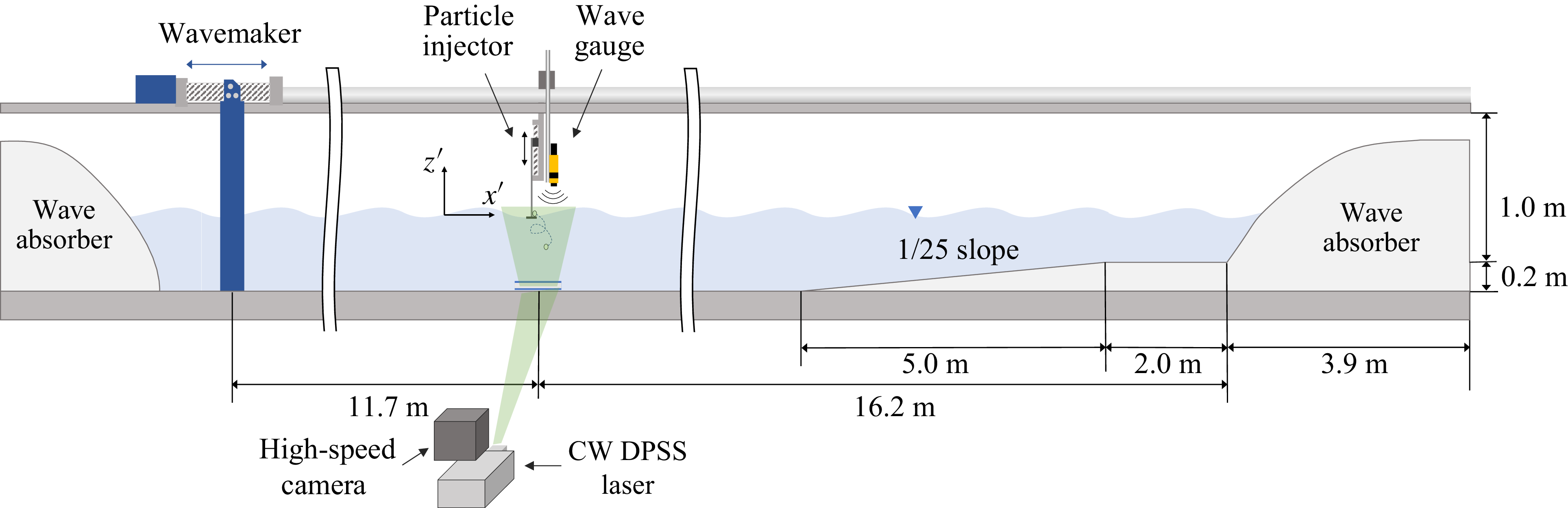

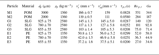

 vs
 ◯
 △
 ◻
 t′=5τp,t

 vs

 vs
 −⟨vz~(zp,t)⟩[z]/vs
 vz−drift

 vs
 ∘
 Nϕ
 rz=⟨wz⟩[ϕ]−minϕwz
 xc
 rz


 Rdrag
 Rwave
 t=5ωτp,t

 rz
 rz=⟨wz⟩[ϕ]−minϕwz
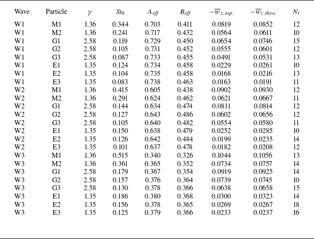
 Nt

 z=zeff


 wx
 wz
 w¯
 wp-p
 δ∗
 ρ(δ)
 ∘
 △
 ◻
 ⋄
 ρ∗
 Ga

 (v′−u′)x∗
 (v′−u′)z∗
 P(f)/(vg′dp)
 fdp/vg′
 vg′=(γ−1)gdp
 dp/(Tvg′)
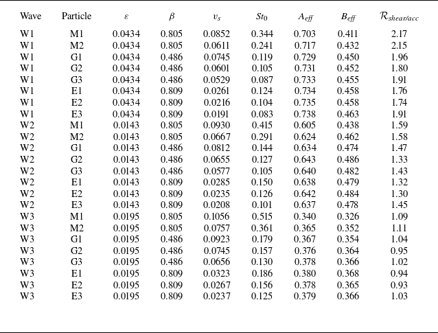
 qz

 Open access

