



1. Introduction
Fluid motion and transport in microgravity are of both fundamental and practical relevance to space thermal management, materials processing, and phase-change technologies. Under terrestrial conditions, gravity provides a natural route for generating buoyancy-driven flow and thereby regulating transport. The canonical example is Rayleigh–Bénard convection, which has long served as a benchmark system for studying thermal turbulence, heat transport, boundary layers and coherent flow organisation (Siggia Reference Siggia1994; Ahlers et al. Reference Ahlers, Grossmann and Lohse2009; Lohse & Xia Reference Lohse and Xia2010; Chillà & Schumacher Reference Chillà and Schumacher2012; Lohse & Shishkina Reference Lohse and Shishkina2023, Reference Lohse and Shishkina2024; Xia et al. Reference Xia, Huang, Xie and Zhang2023, Reference Xia, Chong, Ding and Zhang2025).
In microgravity, by contrast, this mechanism is strongly attenuated, so alternative means of driving fluid motion are required. Mechanical vibration provides a promising alternative, because it is ubiquitous in reduced-gravity environments and can create an effective ‘artificial gravity’ that drives fluid motion and modifies transport processes (Gershuni & Lyubimov Reference Gershuni and Lyubimov1998; Beysens et al. Reference Beysens, Chatain, Evesque and Garrabos2005; Beysens Reference Beysens2006; Lappa Reference Lappa2009; Guo et al. Reference Guo, Wu, Wang, Zhou and Chong2023; Huang et al. Reference Huang, Wu, Guo, Zhao, Wang, Chong and Zhou2024). Correspondingly, theoretical and experimental studies have established vibroconvection as a viable mechanism of heat and mass transport in low-gravity conditions (Mialdun et al. Reference Mialdun, Ryzhkov, Melnikov and Shevtsova2008; Shevtsova et al. Reference Shevtsova, Ryzhkov, Melnikov, Gaponenko and Mialdun2010). However, many low-gravity transport processes involve multiple fluid phases, for which the response to vibration can depend sensitively on phase arrangement and interfacial coupling. These considerations motivate the study of vibroconvection in immiscible two-phase systems, where a deformable interface couples capillarity, phase connectivity and external forcing to the transport process.
Previous studies have established that vibration can substantially alter thermally driven flow. Classical analyses and numerical studies showed that vibration can change convective structures and transport in enclosed fluids under weightless or high-frequency forcing conditions (Gershuni et al. Reference Gershuni, Zhukhovitskii and Yurkov1982; Savino et al. Reference Savino, Monti and Piccirillo1998; Hirata et al. Reference Hirata, Sasaki and Tanigawa2001; Cisse et al. Reference Cisse, Bardan and Mojtabi2004). More recent work has shown that the effect of vibration is not restricted to modulating flow intensity: it can reorganise thermal boundary layers, alter large-scale flow structures and induce distinct transport regimes in thermal convection (Wang et al. Reference Wang, Zhou and Sun2020a ; Guo et al. Reference Guo, Wu, Wang, Zhou and Chong2023; Huang et al. Reference Huang, Guo, Wu, Wang, Chong and Zhou2023, Reference Huang, Wu, Guo, Zhao, Wang, Chong and Zhou2024). Externally forced multiphase systems have likewise been found to exhibit diverse interfacial dynamics, including forcing-dependent symmetry breaking and multiple interfacial states of bubbles (Guan et al. Reference Guan, Tamim, Magoon, Stone and Sáenz2025). These studies indicate that, once a deformable interface is present, the response to vibration is governed not only by bulk convection but also by forcing-selected interfacial states, reflecting a competition between flow reorganisation and interfacial dynamics.
In thermally driven two-phase flows, interfacial physics is central even in the absence of vibration, and the motion of drops and bubbles across sharp interfaces or stratified layers is known to be strongly shaped by interfacial deformation and capillarity (Magnaudet & Mercier Reference Magnaudet and Mercier2020). Early studies of layered thermal convection examined thermal coupling and natural convection in multiple layers of immiscible liquids (Nataf et al. Reference Nataf, Moreno and Cardin1988; Prakash & Koster Reference Prakash and Koster1994), while later experiments addressed turbulent two-layer convection and the coupling between the large-scale circulations across the interface (Xie & Xia Reference Xie and Xia2013). This two-layer turbulent-convection picture has further motivated reduced-order modelling of the coupled large-scale circulations and their reversals (Sun et al. Reference Sun, Xie, Xie, Zhong, Zhang and Xia2024). Recent experiments on thermal convection with two liquid layers and three-layer turbulent thermal convection have further shown that heat transport and flow organisation are strongly affected by the layered configuration and interfacial coupling (Wang et al. Reference Wang, Chen, Wang and Wei2024; Zhao et al. Reference Zhao, Qiu, Zhou, Li, Xi and Xia2024). More recent numerical work showed that interface breakup can arise in two-layer thermally driven turbulence (Liu et al. Reference Liu, Chong, Wang, Ng, Verzicco and Lohse2021a
), that immiscible interfaces can exert a strong influence on transport in layered convection (Liu et al. Reference Liu, Ng, Chong, Lohse and Verzicco2022b
), and that global transport may depend only weakly on
 $\textit{We}$
even though interface fluctuations and interfacial-wave dynamics remain sensitive to it over the Rayleigh–Weber parameter space (Demou et al. Reference Demou, Scapin, Crialesi-Esposito, Costa, Spiga and Brandt2024). In liquid–liquid dispersions, interfacial stabilisation has been shown to control morphology and convective heat-transfer dynamics (Pelusi et al. Reference Pelusi, Scagliarini, Sbragaglia, Bernaschi and Benzi2025b
), while thermally convective emulsions may develop distinct regimes associated with breakup, coalescence and phase inversion (Pelusi et al. Reference Pelusi, Scagliarini, Sbragaglia, Bernaschi and Benzi2025a
).
The organising role of interfaces is also evident in emulsions and other dispersed flows. Interfacial deformation, breakup, coalescence and phase inversion control droplet statistics and bulk transport (Perlekar et al. Reference Perlekar, Biferale, Sbragaglia, Srivastava and Toschi2012; Perazzo et al. Reference Perazzo, Preziosi and Guido2015; Mukherjee et al. Reference Mukherjee, Safdari, Shardt, Kenjeres and van den Akker2019; Soligo et al. Reference Soligo, Roccon and Soldati2019; Bakhuis et al. Reference Bakhuis, Ezeta, Bullee, Marin, Lohse, Sun and Huisman2021; Yi et al. Reference Yi, Toschi and Sun2021, Reference Yi, Wang, van Vuren, Lohse, Risso, Toschi and Sun2022, Reference Yi, Wang, Huisman and Sun2023, Reference Yi, Girotto, Toschi and Sun2024; Ravera et al. Reference Ravera, Dziza, Santini, Cristofolini and Liggieri2021; Ni Reference Ni2024; Sun & Toschi Reference Sun and Toschi2027), while dispersed droplets can modify drag and interfacial transport in wall-bounded and shear-driven flows (Rosti et al. Reference Rosti, Ge, Jain, Dodd and Brandt2019; Hori et al. Reference Hori, Ng, Lohse and Verzicco2023; Su et al. Reference Su, Wang, Zhang, Xu, Wang and Sun2024a , Reference Su, Yi, Zhao, Wang, Xu, Wang and Sun2024b , Reference Su, Zhang, Wang, Yi, Xu, Fan, Wang and Sun2025; Fan et al. Reference Fan, Zhang, Su, Yi, Wang and Sun2025). Related changes in heat transfer and flow fluctuations occur in thermally driven multiphase systems (Wang et al. Reference Wang, Mathai and Sun2019, Reference Wang, Mathai and Sun2020b ; Liu et al. Reference Liu, Chong, Wang, Ng, Verzicco and Lohse2021a ,Reference Liu, Ng, Chong, Lohse and Verzicco b , Reference Liu, Chong, Ng, Verzicco and Lohse2022a ; Qi et al. Reference Qi, Zhao, Fan, Du, Mathai and Sun2026; Meng et al. Reference Meng, Wu, Chong and Zhou2026; Pelusi et al. Reference Pelusi, Sbragaglia, Benzi, Scagliarini, Bernaschi and Succi2021) and in bubbly or particle-laden flows (Lakkaraju et al. Reference Lakkaraju, Schmidt, Oresta, Toschi, Verzicco, Lohse and Prosperetti2011; Mathai et al. Reference Mathai, Lohse and Sun2020; Liu et al. Reference Liu, Chong, Yang, Verzicco and Lohse2022c ). Applications such as inkjet printing likewise underscore the importance of deformation and pinch-off (Lohse Reference Lohse2022). These studies suggest that interfacial deformation and loss of phase connectivity can reorganise transport in vibrated immiscible systems under microgravity.
Vibration-driven immiscible two-phase flow under microgravity can therefore be viewed as a problem in which transport is controlled by the interfacial states selected by the competition between vibration and capillarity. The forcing strength and material contrast are expected to jointly determine the interfacial morphology, while transitions between different interfacial states should, in turn, reorganise the global flow and transport responses. To this end, we carry out direct numerical simulations of an immiscible two-phase layer subjected to a vertical temperature difference and horizontal harmonic vibration under microgravity conditions. We show that the competition between vibration, capillarity and material contrast leads to three interfacial states, and that two critical Weber numbers collapse the corresponding regime transitions. The remainder of the paper is organised as follows. The numerical method is introduced in § 2. The flow morphology, transport responses and regime transitions are presented in § 3. Finally, the main findings are summarised in § 4.
2. Numerical methods
We consider thermally coupled immiscible two-phase flow in a microgravity cell. The thermally coupled two-layer configuration follows the general set-up studied by Liu et al. (Reference Liu, Chong, Yang, Verzicco and Lohse2022b
). The two-dimensional computational domain is a rectangle of width
 $2H$
and height
 $H$
, namely
 $x\in [-H,H]$
and
 $z\in [-H/2,H/2]$
. Additional three-dimensional calculations are performed in a cuboidal domain with dimensions
 $L_x\times L_y\times L_z=2H\times H\times H$
, where
 $z$
is the vertical direction. A constant temperature difference
 $\varDelta$
is imposed in the vertical direction, with the top wall maintained at
 $-\varDelta /2$
and the bottom wall at
 $\varDelta /2$
. Since the present study concerns the microgravity regime, steady gravitational buoyancy is omitted and a horizontal harmonic vibration
 $A\cos (\varOmega t)\hat {\boldsymbol{e}}_x$
is imposed to act as an artificial driving. In the non-inertial frame associated with the imposed vibration, an inertial acceleration in the horizontal direction is introduced into the system, thereby generating vibroconvection (Gershuni & Lyubimov Reference Gershuni and Lyubimov1998; Shevtsova et al. Reference Shevtsova, Ryzhkov, Melnikov, Gaponenko and Mialdun2010; Huang et al. Reference Huang, Wu, Guo, Zhao, Wang, Chong and Zhou2024). Here,
 $A$
and
 $\varOmega$
denote the dimensional vibration amplitude and angular frequency, respectively, and
 $\hat {\boldsymbol{e}}_x$
is the unit vector in the horizontal direction. We employ a one-fluid description to simulate the immiscible two-phase system, in which the two fluids are distinguished by a phase indicator
 $C$
, with
 $C=0$
in fluid 0 and
 $C=1$
in fluid 1. The treatment of thermally coupled multiphase transport follows in the spirit of Liu et al. (Reference Liu, Ng, Chong, Lohse and Verzicco2021b
, Reference Liu, Chong, Yang, Verzicco and Lohse2022b
). All quantities are made dimensionless with respect to the cell height
 $H$
, the imposed temperature difference
 $\varDelta$
, the vibration-induced velocity scale
 $U_v=\alpha _0 A\varOmega \Delta$
, the time scale
 $H/U_v$
and the pressure scale
 $\rho _0U_v^2$
. In this scaling,
 $\alpha _0$
denotes the reference thermal-expansion coefficient of fluid 0. The resulting non-dimensional governing equations for this system read
 \begin{equation} \boldsymbol{\nabla }\boldsymbol{\cdot }\boldsymbol{u}=0, \end{equation}
 \begin{equation} \tilde {\rho }\left (\partial _t\boldsymbol{u}+\boldsymbol{u}\boldsymbol{\cdot }\boldsymbol{\nabla }\boldsymbol{u}\right ) =-\boldsymbol{\nabla }\!p+\sqrt {\frac {\textit{Pr}}{2\textit{Ra}_{vib}}}\boldsymbol{\nabla }\boldsymbol{\cdot }\big [\tilde {\mu }\big (\boldsymbol{\nabla }\boldsymbol{u}+\boldsymbol{\nabla }\boldsymbol{u}^{T}\big )\big ] +\boldsymbol{F}_{st}+\boldsymbol{G}_{vib}, \end{equation}
 \begin{equation} \tilde {\rho }\tilde {c}_p\left (\partial _t \theta +\boldsymbol{u}\boldsymbol{\cdot }\boldsymbol{\nabla }\theta \right ) =\frac {1}{\sqrt {2\textit{Pr}\textit{Ra}_{vib}}}\boldsymbol{\nabla }\boldsymbol{\cdot }\big (\tilde {k}\boldsymbol{\nabla }\theta \big ), \end{equation}
 \begin{equation} \partial _t C+\boldsymbol{u}\boldsymbol{\cdot }\boldsymbol{\nabla }C=0. \end{equation}
Here, the capillary force is written as
 \begin{equation} \boldsymbol{F}_{st}=\frac {1}{\textit{We}}\,\kappa \delta _s\hat {\boldsymbol{n}}, \end{equation}
where
 $\hat {\boldsymbol{n}}=\boldsymbol{\nabla }C/|\boldsymbol{\nabla }C|$
is the unit normal directed from fluid 0 to fluid 1,
 $\kappa =-\boldsymbol{\nabla }\boldsymbol{\cdot }\hat {\boldsymbol{n}}$
is the interfacial curvature and
 $\delta _s=|\boldsymbol{\nabla }C|$
is the surface delta distribution in the continuum-surface-force representation, while the vibration forcing is
 \begin{equation} \boldsymbol{G}_{vib}=a^{-1}\tilde {\rho }\tilde {\alpha }\,\theta \,\cos \big (a^{-1}t\big )\hat {\boldsymbol{e}}_x. \end{equation}
Here,
 $\boldsymbol{u}$
is the dimensionless velocity field,
 $p$
is the dimensionless pressure and
 $\theta$
is the dimensionless temperature. The capillary contribution is represented by
 $\boldsymbol{F}_{st}$
and the vibrational forcing by
 $\boldsymbol{G}_{vib}$
. Surface tension is assumed to be temperature-independent, so thermocapillary (Marangoni) stresses are neglected. This isolates the competition between thermovibrational forcing and capillary restoration, and the results apply most directly when thermocapillary effects are weak. To assess this approximation, we use
 $H$
as the characteristic tangential length and compare the thermocapillary stress
 $|\mathrm{d}\sigma /\mathrm{d}T|\Delta T_{\parallel }/H$
with the reference thermovibrational inertial stress
 $\rho _0U_v^2$
, defining
 \begin{equation} \varPi _M=\frac {|\mathrm{d}\sigma /\mathrm{d}T|\,\Delta T_{\parallel }}{\rho _0U_v^2H} =\frac {|\mathrm{d}\sigma /\mathrm{d}T|\,\Delta T_{\parallel }H}{2\rho _0\textit{Ra}_{vib}\nu _0\kappa _0}. \end{equation}
Here,
 $\Delta T_{\parallel }$
is the dimensional temperature variation along the interface, distinct from the imposed wall-temperature difference
 $\varDelta$
. Thus,
 $\varPi _M\ll 1$
indicates a weak thermocapillary contribution on the cell scale. Water–silicone oil (Peters & Arabali Reference Peters and Arabali2013) and 20 cSt silicone oil–Fluorinert (Someya & Munakata Reference Someya and Munakata2005) are examples of immiscible fluid pairs studied experimentally. Taking these systems as examples, we make illustrative estimates using representative reference-fluid properties and assumed interfacial-tension temperature coefficients. For
 $\textit{Ra}_{vib}=10^5$
and
 $H=10\,\mathrm{cm}$
, we obtain
 $\varPi _M/\Delta T_{\parallel }\approx 0.50$
and
 $6.6\times 10^{-3}\,\mathrm{K^{-1}}$
, respectively, using water and silicone oil as the reference fluids. The latter estimate remains small for interfacial temperature variations of several Kelvin, whereas the former requires much smaller variations. These order-of-magnitude estimates illustrate the approximation’s scope; the simulations use idealised material properties rather than those of either of the experimental fluid pair, with only the thermal-expansion coefficients differing between phases. Finite Marangoni forcing may modify the interfacial dynamics, transition thresholds and heat transport.
All dimensionless material properties, denoted by
 $\tilde {q}$
, are defined uniformly as
 \begin{equation} \tilde {q}=C\lambda _q+(1-C), \end{equation}
where
 $\lambda _q=q_1/q_0$
is the ratio of the material property
 $q$
in fluid 1 to the reference value
 $q_0$
, with
 $q\in \{\rho ,\mu ,k,c_p,\alpha \}$
. The dimensionless vibration amplitude is
 $a=\alpha _0A\Delta /H$
, so that the dimensionless forcing frequency under the present velocity scale is
 $\omega \equiv \varOmega H/U_v=a^{-1}$
. The principal dimensionless control parameters are
 \begin{equation} a=\frac {\alpha _0 A \Delta }{H},\qquad \textit{Ra}_{vib}=\frac {(\alpha _0 A \varOmega \Delta H)^2}{2\nu _0\kappa _0}, \end{equation}
 \begin{equation} \textit{Pr}=\frac {\nu _0}{\kappa _0},\qquad \textit{We} =\frac {\rho _0(\alpha _0 A\varOmega \Delta )^2H}{\sigma }, \end{equation}
where
 $A$
and
 $\varOmega$
denote the dimensional vibration amplitude and angular frequency, respectively. In what follows, the thermal-expansion contrast is denoted by
 $\alpha _1/\alpha _0$
. Unlike the classical Rayleigh number governing gravitational convection,
 $\textit{Ra}_{vib}=U_v^2H^2/(2\nu _0\kappa _0)$
measures thermovibrational forcing relative to viscous and thermal diffusion. In the high-frequency limit, it characterises the induced mean flow (Gershuni & Lyubimov Reference Gershuni and Lyubimov1998; Lappa Reference Lappa2009), while
 $\omega$
, or equivalently
 $a=\omega ^{-1}$
under the present scaling, remains an independent parameter governing the temporal response. For the main parameter sweep, we fix
 $\textit{Ra}_{vib}=10^5$
,
 $\textit{Pr}=4.38$
and
 $a=0.01$
, vary
 $\textit{We}$
over
 $0.1\leqslant \textit{We} \leqslant 3000$
, and consider
 $\alpha _1/\alpha _0=3,4,5,6,7$
. All other material-property ratios are unity.
The governing equations are solved numerically using an in-house code developed based on the open-source Basilisk C framework (Popinet Reference Popinet2013). The incompressible Navier–Stokes equations are advanced with the centred projection method, while the interface is captured with the geometrical volume-of-fluid method and the balanced-force treatment of surface tension (Popinet Reference Popinet2009, Reference Popinet2015). The temperature field is treated as a conservative scalar with variable volumetric heat capacity and thermal conductivity. The coupled two-phase implementation is benchmarked against the two-layer thermal-convection results of Liu et al. (Reference Liu, Chong, Yang, Verzicco and Lohse2022b
) (figure 1). The normalised Nusselt numbers at
 $\textit{We}=20$
and 200 differ from the reference values by
 $0.67\,\%$
and
 $1.04\,\%$
, respectively, while the
 $\textit{We}=20$
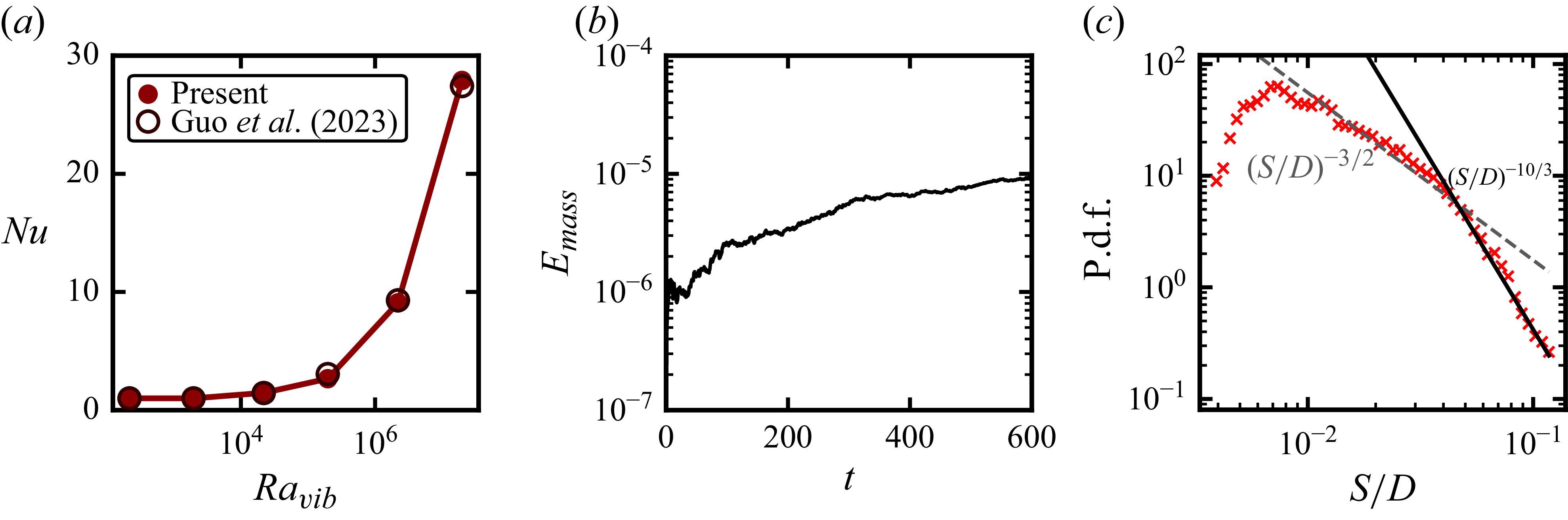
temperature field reproduces the reported interfacial deformation and thermal structure. Additional tests of thermovibrational forcing, stationary two-layer conduction and interface capturing during breakup are reported in Appendix A.
Validation against the two-layer thermal-convection results of Liu et al. (Reference Liu, Chong, Yang, Verzicco and Lohse2022b
). (
 $a$
) Nusselt number normalised by the corresponding single-phase value,
 $\textit{Nu}/\textit{Nu}_s$
, as a function of
 $\textit{We}$
. (
 $b$
) Present values and their relative differences from the reference data at
 $\textit{We}=20$
and 200. Instantaneous temperature fields at
 $\textit{We}=20$
from (
 $c$
) the present simulation and (
 $d$
) Liu et al. (Reference Liu, Chong, Yang, Verzicco and Lohse2022b
). The black contour in panel (
 $c$
) denotes the liquid–liquid interface at
 $C=0.5$
.

Second, we suppress motion and vibration, and consider stationary conduction through two equal-depth immiscible layers,
 $H_0=H_1=H/2$
. With all property ratios except
 $\lambda _k=k_1/k_0$
set to unity, we test
 $\lambda _k=0.5$
, 1, 2 and 5. For the boundary conditions, the top and bottom plates at
 $z=\pm H/2$
are rigid no-slip walls. The lateral boundaries are periodic: in the two-dimensional simulations, this applies to the
 $x$
direction, whereas in the three-dimensional simulations, both the
 $x$
and
 $y$
directions are periodic. In the present non-dimensionalisation, the wall temperatures are fixed at
 $\theta =-1/2$
on the top wall and
 $\theta =1/2$
on the bottom wall. For the initial condition, the flow is initialised from a quiescent two-layer configuration. In two dimensions, the initial interface is prescribed through the phase indicator as
 \begin{equation} C(x,z,0)=\mathcal{H}(H_{\textit{layer}}-z), \end{equation}
with the analogous three-dimensional initialisation
 $C(x,y,z,0)=\mathcal{H}(H_{\textit{layer}}-z)$
. Here,
 $\mathcal{H}(\boldsymbol{\cdot })$
is the Heaviside function and
 $H_{\textit{layer}}$
determines the initial layer height. The dispersed phase is initially placed in the lower layer with a fixed volume fraction
 \begin{equation} \phi _d=\frac {1}{|\mathcal{D}|}\int _{\mathcal{D}} C(\boldsymbol{x},0)\,\mathrm{d}\mathcal{D}=0.2, \end{equation}
where
 $\mathcal{D}$
denotes the computational domain, with
 $\mathrm{d}\mathcal{D}$
representing an area element in two dimensions and a volume element in three dimensions. Since the dimensionless cell height is unity, this corresponds to
 $H_{\textit{layer}}=-0.3$
in the domain
 $z\in [-1/2,1/2]$
; the resulting
 $20\,\%$
dispersed-phase loading is comparable to the minority-layer fractions considered in previous two-layer thermal-convection simulations (Liu et al. Reference Liu, Chong, Yang, Verzicco and Lohse2022b
). The initial temperature field is taken to be a linear conductive profile plus a small random perturbation,
 \begin{equation} \theta (x,z,0)=-z+\epsilon \,\xi (x,z), \end{equation}
with the corresponding three-dimensional form
 $\theta (x,y,z,0)=-z+\epsilon \,\xi (x,y,z)$
. Here,
 $\xi$
is a zero-mean random field and
 $\epsilon$
is a small perturbation amplitude. The initial velocity field is set to
 $\boldsymbol{u}=0$
.
For spatial discretisation, the parameter-sweep simulations use a uniform
 $512\times 256$
grid for all fields. Within the Basilisk multigrid framework, the three-dimensional validation cases use a
 $256\times 128\times 128$
grid for velocity, pressure and temperature, and a
 $512\times 256\times 256$
grid for the VOF field. Grid-refinement tests based on
 $M_{\textit{det}}$
,
 $\textit{Nu}$
and
 $\textit{Re}$
support the adequacy of the production grid (Appendix B). The time step is adjusted dynamically from the CFL restriction; for low-
 $\textit{We}$
cases, a smaller CFL cap is used to improve robustness. In addition, a smooth start-up factor is applied in low-
 $\textit{We}$
cases to avoid spurious initial transients. Statistics are accumulated only after the flow reaches a statistically stationary state and span at least 600 dimensionless time units, with time scaled by
 $H/U_v$
. We assess convergence by comparing the means over the first and second halves of each sampling interval; the resulting relative drift does not exceed 2 %.
(
 $a$
)–(
 $c$
) Three-dimensional visualisations of the dispersed-phase morphology at Weber numbers (
 $a$
)
 $\textit{We}=0.1$
, (
 $b$
)
 $\textit{We}=2$
and (
 $c$
)
 $\textit{We}=1000$
. The panels show the transition from a stratified-layer state to an interfacial-bulging state and then to a droplet-dispersed state. (
 $d$
)–(
 $f$
) Corresponding three-dimensional temperature fields for the same three Weber numbers, showing the accompanying reorganisation of the thermal structure. (
 $g$
) Nusselt number
 $\textit{Nu}$
as a function of
 $\textit{We}$
for different thermal-expansion contrasts
 $\alpha _1/\alpha _0$
from the two-dimensional parameter sweep, together with representative three-dimensional results. (
 $h$
) Reynolds number
 $\textit{Re}$
as a function of
 $\textit{We}$
for the same cases. All cases are performed at fixed
 $\textit{Ra}_{vib}=10^5$
and vibration amplitude
 $a=0.01$
.

3. Results and discussion
We first examine the global flow and heat-transport characteristics of the vibrated two-phase system. Figure 2(a–c) shows three-dimensional distributions of the dispersed phase at three representative Weber numbers and figure 2(d–f) shows the corresponding three-dimensional temperature fields. At low Weber number (figure 2
a,d;
 $\textit{We}=0.1$
), capillarity suppresses large interfacial deformation and the two fluids remain nearly stratified, so the temperature field retains a layered structure.
As
 $\textit{We}$
increases (figure 2
b,e;
 $\textit{We}=2$
), the capillary constraint is weakened and the interface develops pronounced bulging, accompanied by a stronger distortion of the thermal field near the interface. At much larger
 $\textit{We}$
(figure 2
c, f;
 $\textit{We}=1000$
), the dispersed phase is no longer anchored to the initial layer and forms a droplet-dispersed morphology, producing a different thermal organisation around the mobile dispersed structures. These snapshots therefore suggest three distinct morphological states: a stratified-layer state, an interfacial-bulging state and a droplet-dispersed state, consistent with the broader observation that interfacial structure can organise distinct transport states in thermally driven multiphase flows (Liu et al. Reference Liu, Chong, Yang, Verzicco and Lohse2022b
; Pelusi et al. Reference Pelusi, Scagliarini, Sbragaglia, Bernaschi and Benzi2025b
). Representative time-dependent evolution within these states is shown in supplementary movies 1–3 available at https://doi.org/10.1017/jfm.2026.12243 at
 $\textit{We}=1$
, 10 and 1000, respectively.
The change in flow structure can also be reflected in the transport response. In the present work, the reported Nusselt number is taken as
 $\textit{Nu}=(\textit{Nu}_{\textit{top}}+\textit{Nu}_{\textit{bot}})/2$
, where the wall values are defined from the conductivity-weighted heat flux as
 \begin{equation} \textit{Nu}_{\textit{top},\textit{bot}}= \frac {\left \langle -k\,\partial _z T\right \rangle _{\textit{top},\textit{bot}}} {k_{\textit{eff}}\Delta /H}. \end{equation}
Here,
 $\langle \boldsymbol{\cdot }\rangle$
denotes averaging along the corresponding wall,
 $k_{\textit{eff}}=H/(H_0/k_0+H_1/k_1)$
is the effective conductivity of the initial two-layer conductive state, and
 $H_0$
and
 $H_1$
are the initial thicknesses of fluids 0 and 1, following the same series-conduction normalisation used for biphasic thermal convection (Wang et al. Reference Wang, Mathai and Sun2020b
). Since
 $k_1/k_0=1$
in the present cases,
 $k_{\textit{eff}}=k_0$
; in dimensionless form, this reduces to
 $\textit{Nu}_{\textit{top},\textit{bot}}=\langle -\tilde {k}\partial _z\theta \rangle _{\textit{top},\textit{bot}}$
. The Reynolds number is defined as
 $\textit{Re}=U_{rms}H/\nu _0$
, with
 $U_{rms}=\langle \boldsymbol{u}\boldsymbol{\cdot }\boldsymbol{u}\rangle _{V,t}^{1/2}$
(Zhang et al. Reference Zhang, Zhou and Sun2017; Wu et al. Reference Wu, Wang, Chong, Dong, Sun and Zhou2022).
The corresponding transport data in figures 2(g) and 2(h) exhibit three distinct trends, each associated with one of the flow states identified earlier. In the stratified-layer state (figure 2
a,d), the system remains essentially a two-layer flow and the temperature field retains a layered structure. Over this interval, the transport response remains associated with the stratified thermal structure, while
 $\textit{Re}$
changes only weakly. When interfacial bulging develops (figure 2
b,e), hot fluid is lifted and cold fluid penetrates downward, opening an efficient cross-interface transport channel and producing the sharp rise of
 $\textit{Nu}$
. The lifted dispersed phase, however, intrudes into the bulk and obstructs the previously coherent circulation, converting part of the motion into interfacial deformation and confined recirculation; as a result,
 $\textit{Re}$
decreases. In the droplet-dispersed state (figure 2
c, f), detached droplets move vertically through the cell and carry heat between the hot and cold regions, thereby enhancing vertical heat transport and keeping
 $\textit{Nu}$
high. At the same time, the coherent large-scale circulation is further broken into local recirculation, interfacial motion and droplet-scale motion, so that the volume-averaged
 $\textit{Re}$
remains low, consistent with previous observations that dispersed droplets or bubbles can modify vortical structures, velocity fluctuations and dissipation in multiphase thermal flows (Magnaudet & Eames Reference Magnaudet and Eames2000; Yuge & Hagiwara Reference Yuge and Hagiwara2004; Lakkaraju et al. Reference Lakkaraju, Schmidt, Oresta, Toschi, Verzicco, Lohse and Prosperetti2011; Qi et al. Reference Qi, Zhao, Fan, Du, Mathai and Sun2026). The representative three-dimensional results show a slightly higher
 $\textit{Nu}$
and an earlier decrease in
 $\textit{Re}$
than their two-dimensional counterparts (figure 2
g,h). A similar dimensional trend has been reported in Rayleigh–Bénard convection, where planar confinement strengthens the large-scale circulation and increases
 $\textit{Re}$
without necessarily enhancing
 $\textit{Nu}$
(van der Poel et al. Reference van der Poel, Stevens and Lohse2013). In the present system, spanwise freedom may weaken the coherent circulation while allowing spatially distributed interfacial and droplet motion to sustain vertical heat transport. Thus,
 $\textit{Nu}$
is controlled mainly by the availability of cross-interface heat pathways, whereas
 $\textit{Re}$
measures the coherence of the global flow. Although
 $\textit{Nu}$
and
 $\textit{Re}$
depend on the vibration frequency even at fixed
 $\textit{Ra}_{vib}$
, the sequence of interfacial states is retained over the tested range (Appendix C). To characterise the three states locally, we examine the wall-normal profiles of the temperature and vertical-velocity fluctuations,
 \begin{equation} T_{\textit{rms}}(z)=\left \langle \left [T-\langle T\rangle _{x,t}\right ]^2\right \rangle _{x,t}^{1/2},\qquad w_{\textit{rms}}(z)=\left \langle \left [w-\langle w\rangle _{x,t}\right ]^2\right \rangle _{x,t}^{1/2}. \end{equation}
Here,
 $\langle \boldsymbol{\cdot }\rangle _{x,t}$
denotes horizontal and temporal averaging over the statistically stationary interval. Figure 3 provides distinct local signatures of the three states. In the stratified state,
 $w_{\textit{rms}}$
is localised near the initial interface and
 $T_{\textit{rms}}$
varies markedly across it. Bulging extends both fluctuations into the bulk, whereas the droplet-dispersed state exhibits broader profiles that are nearly symmetric about the midplane. We next examine the transition thresholds separating these states.
Wall-normal profiles of (
 $a$
)
 $T_{\textit{rms}}$
and (
 $b$
)
 $w_{\textit{rms}}$
for
 $\alpha _1/\alpha _0=4$
. Blue, orange and red denote the stratified-layer (
 $\textit{We}=0.1$
, 0.3 and 0.6), interfacial-bulging (
 $\textit{We}=15$
, 20 and 30) and droplet-dispersed (
 $\textit{We}=300$
, 1000 and 3000) states, respectively. Solid curves bound the shaded range in each state and the intermediate case is dash-dotted. The horizontal dashed line marks the initial interface position
 $z/H=-0.3$
.

To quantify these transitions, we define
 $\mathcal{D}_+=\{\boldsymbol{x}\in \mathcal{D}:z\gt z_0\}$
as the portion of the computational domain above the reference height
 $z_0$
. The elevated dispersed-phase fraction is then given by
 \begin{equation} M_{\textit{det}}(t)= \frac {\displaystyle \int _{\mathcal{D}_+} C(\boldsymbol{x},t)\,\mathrm{d}\boldsymbol{x}} {\displaystyle \int _{\mathcal{D}} C(\boldsymbol{x},t)\,\mathrm{d}\boldsymbol{x}}. \end{equation}
Here,
 $\mathrm{d}\boldsymbol{x}$
denotes an area element in two dimensions and a volume element in three dimensions. In the present geometry,
 $z_0$
coincides with the initial interface position, namely
 $z_0=-0.3$
. The reported value is obtained by evaluating
 $M_{\textit{det}}(t)$
from instantaneous fields and averaging over the statistically stationary interval. We use this quantity to characterise the degree of bulging of the dispersed phase above the reference height. By definition,
 $M_{\textit{det}}=0$
corresponds to an ideal layered state in which the dispersed phase remains below the reference height
 $z_0$
. At the other extreme, once the detached droplet is no longer trapped near the lower layer, it travels back and forth between the two plates under the vibration-driven flow; as a result, its time-averaged vertical distribution becomes approximately uniform, and one then expects
 $M_{\textit{det}}\approx 0.8$
because the subdomain
 $z\gt z_0$
occupies
 $80\,\%$
of the cell height in the present geometry.
(
 $a$
) Schematic of the onset of interfacial bulging in the vibrated two-phase layer. A weakly perturbed interface,
 $z_s(x)=z_0+\eta \cos (k_m x)$
, becomes unstable when the thermovibrational pressure difference
 $\Delta p_{vib}$
overcomes the capillary restoring stress represented by
 $\Delta p_{\sigma }$
. (
 $b$
) Elevated dispersed-phase fraction
 $M_{\textit{det}}$
as a function of
 $\textit{We}$
for different thermal-expansion contrasts
 $\alpha _1/\alpha _0$
, from which the critical Weber number
 $\textit{We}_{c,\textit{bulging}}$
for interfacial bulging is determined. Representative three-dimensional data at
 $\alpha _1/\alpha _0=5$
are included for comparison. Here,
 $M_{\textit{det}}$
denotes the fraction of the dispersed phase located above the reference height
 $z_0$
. (
 $c$
) Critical Weber number
 $\textit{We}_{c,\textit{bulging}}$
plotted against
 $\alpha _1/\alpha _0$
. The decrease of
 $\textit{We}_{c,\textit{bulging}}$
with increasing
 $\alpha _1/\alpha _0$
is compared with the scaling prediction
 $\textit{We}_{c,\textit{bulging}}\sim (\alpha _1/\alpha _0-1)^{-2}$
(grey curve).

The measured
 $M_{\textit{det}}$
is shown in figure 4(b) as a function of
 $\textit{We}$
for different
 $\alpha _1/\alpha _0$
. For each thermal-expansion ratio
 $\alpha _1/\alpha _0$
,
 $M_{\textit{det}}$
remains small in the stratified-layer regime and increases once interfacial bulging develops. Here,
 $\textit{We}_{c,\textit{bulging}}$
is identified from figure 4(b) using the small threshold
 $M_{\textit{det}}=0.03$
, which separates the nearly stratified branch from the bulging branch. The same elevated dispersed-phase fraction is also used to define the droplet-detachment threshold,
 $\textit{We}_{c,\textit{det}}$
, using
 $M_{\textit{det}}=0.79$
, which marks the transition to the droplet-dispersed branch. This second threshold will be discussed later. We first focus on the onset of interfacial bulging. Figure 4(c) shows that
 $\textit{We}_{c,\textit{bulging}}$
decreases monotonically as
 $\alpha _1/\alpha _0$
increases, indicating that a larger thermal-expansion contrast destabilises the interface at a smaller Weber number.
To explain this trend, we estimate the onset condition from a balance between the thermovibrational pressure difference and capillary restoring stress at the interface (figure 4
a). When the two fluids have different thermal-expansion coefficients, the imposed vibration produces unequal thermovibrational responses on the two sides of the interface. The dimensional relative velocity can be estimated as
 $U_{\textit{int}}^*\sim (\alpha _1-\alpha _0)A\varOmega \Delta T$
, or equivalently,
 $U_{\textit{int}}^*\sim (\alpha _1/\alpha _0-1)U_v$
with
 $U_v=\alpha _0A\varOmega \Delta T$
.
For a weakly perturbed interface
 $z_s^*(x^*)=z_0^*+\eta ^*\cos (k_m^*x^*)$
, the thermovibrational pressure difference has the dimensional scale
 \begin{equation} \Delta p_{vib}^{*}\sim \rho _0 U_{\textit{int}}^{*2}\frac {\eta ^{*}}{H} \sim \rho _0U_v^2\left (\frac {\alpha _1}{\alpha _0}-1\right )^2\frac {\eta ^{*}}{H} . \end{equation}
The capillary restoring pressure is set by the curvature perturbation. Since
 $\kappa ^*\sim k_m^{*2}\eta ^*$
for this mode, its dimensional scale is
 \begin{equation} \Delta p_{\sigma }^{*}\sim \sigma k_m^{*2}\eta ^{*} . \end{equation}
At the onset of interfacial bulging, these two dimensional pressure scales balance,
 \begin{equation} \rho _0U_v^2\left (\frac {\alpha _1}{\alpha _0}-1\right )^2\frac {\eta ^{*}}{H} \sim \sigma k_m^{*2}\eta ^{*} . \end{equation}
Introducing
 $\textit{We}=\rho _0U_v^2H/\sigma$
and
 $k_m=k_m^*H$
, this balance gives
 \begin{equation} \textit{We}_{c,\textit{bulging}}\left (\frac {\alpha _1}{\alpha _0}-1\right )^2\sim k_m^2, \qquad \textit{We}_{c,\textit{bulging}}\sim k_m^2\left (\frac {\alpha _1}{\alpha _0}-1\right )^{-2}. \end{equation}
For the present fixed geometry and initial layer height, the lowest mode, corresponding to the dimensionless wavenumber
 $k_m=k_m^{*}H\simeq 1$
, is expected to become unstable first, because it requires the smallest capillary restoring pressure in the above-mentioned balance. This is also the onset mode observed in the simulations. The corresponding wavenumber factor can therefore be absorbed into the prefactor, giving
 \begin{equation} \textit{We}_{c,\textit{bulging}}\sim \left (\frac {\alpha _1}{\alpha _0}-1\right )^{-2}. \end{equation}
This reduced form provides a direct comparison with the critical Weber numbers extracted from the elevated dispersed-phase fraction. As shown in figure 4(c), the measured thresholds follow the predicted decrease with increasing
 $\alpha _1/\alpha _0$
, indicating that the onset of interfacial bulging is well described by the pressure–capillary balance. It should be noted that this scaling estimate retains only the interfacial pressure imbalance caused by the thermal-expansion mismatch, while neglecting temperature-induced density variations within each layer, which may also contribute to the thermovibrational pressure variation.
(
 $a$
) Schematic of the second transition from interfacial bulging to droplet detachment. The lifted liquid volume
 $V_d$
is driven by the effective thermovibrational force, while the capillary force retaining the remaining neck is characterised by a contact length
 $L_n$
. (
 $b$
) Measured
 $V_d$
at the droplet-detachment threshold
 $\textit{We}_{c,\textit{det}}$
as a function of the thermal-expansion contrast
 $\alpha _1/\alpha _0$
. The shaded band denotes the mean value with a
 $\pm 10\,\%$
variation, showing that
 $V_d$
varies only weakly over the range considered. (
 $c$
) Droplet-detachment threshold
 $\textit{We}_{c,\textit{det}}$
as a function of
 $\alpha _1/\alpha _0$
. The grey curve shows the leading-order scaling
 $C_f(\alpha _1/\alpha _0-1)^{-2}$
with fitted prefactor
 $C_f$
, while the dashed curve includes the geometric correction
 $L_nV_d^{-1}(\alpha _1/\alpha _0-1)^{-2}$
, with
 $V_d$
measured at the detachment threshold and
 $L_n$
treated as approximately constant.

We next consider the second transition point, at which the lifted dispersed-phase structure loses its neck connection to the lower layer. This transition corresponds to the change from the interfacial-bulging state to droplet detachment. At this stage, the interface is no longer a small-amplitude perturbation, but has formed a finite-amplitude elevated liquid structure that remains connected to the lower layer through a thin neck. Droplet detachment occurs when this neck connection is broken (figure 5
a). The corresponding time-dependent evolution at
 $\textit{We}=200$
is shown in supplementary movie 4. Such loss of interfacial connectivity is known to reorganise multiphase dynamics (Soligo et al. Reference Soligo, Roccon and Soldati2019; Liu et al. Reference Liu, Chong, Wang, Ng, Verzicco and Lohse2021a
). The controlling balance is therefore different from that for the first transition: interfacial bulging is governed by a pressure–capillary balance for a weak deformation, whereas droplet detachment is governed by a force balance between the thermovibrational force acting on the lifted liquid volume and the capillary force retaining the remaining neck.
The thermovibrational force responsible for detachment can be written schematically as the sum of two contributions,
 $F_{{vib}}^{*}\sim F_{\textit{base}}^{*}+F_{\textit{contrast}}^{*}$
. The baseline term represents the phase-common thermovibrational response and has the reference inertial-force scale
 $F_{\textit{base}}^{*}\sim (\rho _0U_v^2/H)V_d^{*}$
. The second term arises from the mismatch of the thermovibrational response across the interface. This mismatch produces an oscillatory body-force difference of order
 $\Delta f_{{vib},\textit{inst}}^{*}\sim \rho _0(\alpha _1-\alpha _0)A\varOmega ^2\Delta T$
and a relative vibration velocity
 $U_{\textit{rel}}^{*}\sim (\alpha _1-\alpha _0)A\varOmega \Delta T$
. Since the instantaneous contribution changes sign over a vibration period, the leading averaged inertial contribution is quadratic in
 $U_{\textit{rel}}^{*}$
, giving
 $F_{\textit{contrast}}^{*}\sim (\rho _0U_v^2/H)(\alpha _1/\alpha _0-1)^2V_d^{*}$
. Thus, the contrast-dependent term sets the leading dependence of the detachment threshold on
 $\alpha _1/\alpha _0$
, while the baseline and lower-order terms are absorbed into the prefactor. The detailed derivation of these force scales is given in Appendix D.
The reduced detachment balance therefore involves the following dimensional force scales:
 \begin{equation} F_{\textit{contrast}}^{*} \sim \frac {\rho _0U_v^2}{H} \left (\frac {\alpha _1}{\alpha _0}-1\right )^2V_d^{*}, \qquad F_{\sigma }^{*}\sim \sigma L_n^{*}, \end{equation}
where
 $V_d^{*}$
is the dimensional lifted volume and
 $L_n^{*}$
is the dimensional contact length of the neck. Balancing these forces, and using
 $\textit{We}=\rho _0U_v^2H/\sigma$
,
 $L_n=L_n^{*}/H$
and
 $V_d=V_d^{*}/H^3$
gives
 \begin{equation} \textit{We}_{c,\textit{det}}\sim \frac {L_n}{V_d}\left (\frac {\alpha _1}{\alpha _0}-1\right )^{-2}. \end{equation}
Here, the ratio
 $L_n/V_d$
is retained as the geometric factor controlling the capillary retention of the neck. In the two-dimensional calculations, the force balance is interpreted per unit span, so the capillary factor associated with the neck is an order-one constant and the measured
 $V_d$
is the lifted area, equivalently, the lifted volume per unit span. In three dimensions,
 $L_n$
denotes the contact-line length of the neck and
 $V_d$
the lifted volume. The three-dimensional calculation in figure 2(c) indicates weak spanwise development during detachment; for the present spanwise extent, this gives an approximately constant
 $L_n$
of order unity, approximately
 $2$
if the two sides of the neck are counted. Thus, the difference between the two- and three-dimensional measures mainly affects the prefactor. As shown in figure 5(b),
 $V_d$
at the detachment threshold changes only weakly with
 $\alpha _1/\alpha _0$
. Thus, the leading dependence reduces to
 $\textit{We}_{c,\textit{det}}\sim (\alpha _1/\alpha _0-1)^{-2}$
. Figure 5(c) confirms this trend: the reduced scaling captures the systematic decrease of
 $\textit{We}_{c,\textit{det}}$
, while including the measured
 $V_d^{-1}$
correction gives an almost overlapping curve. The second transition is therefore controlled mainly by the same contrast-dependent forcing as the first transition, with a different prefactor set by finite-amplitude detachment and neck retention. More generally, the offset between the two thresholds scales as
 $L_n/(V_d k_m^2)$
and need not remain constant when the domain geometry is varied, because changes in the domain width, height or spanwise extent may alter the onset mode
 $k_m$
, the lifted volume or the neck geometry.
(
 $a$
) Nusselt number
 $\textit{Nu}$
and (
 $b$
) Reynolds number
 $\textit{Re}$
as functions of
 $\textit{We}/\textit{We}_{c,\textit{bulging}}$
for different thermal-expansion contrasts
 $\alpha _1/\alpha _0$
. (
 $c$
) Nusselt number
 $\textit{Nu}$
and (
 $d$
) Reynolds number
 $\textit{Re}$
as functions of
 $\textit{We}/\textit{We}_{c,\textit{det}}$
. The coloured background indicates the three regimes: stratified-layer, interfacial-bulging and droplet-dispersed states. The dotted vertical line marks the corresponding normalised threshold, namely
 $\textit{We}/\textit{We}_{c,\textit{bulging}}=1$
in panels (
 $a$
) and (
 $b$
), and
 $\textit{We}/\textit{We}_{c,\textit{det}}=1$
in panels (
 $c$
) and (
 $d$
).

To assess how these two thresholds organise the global transport response, we replot the data against the corresponding normalised Weber numbers. Figure 6(a,b) shows
 $\textit{Nu}$
and
 $\textit{Re}$
as functions of
 $\textit{We}/\textit{We}_{c,\textit{bulging}}$
. Under this normalisation, the first transition is aligned near
 $\textit{We}/\textit{We}_{c,\textit{bulging}}=1$
, so that the onset of interfacial bulging can be compared directly across different thermal-expansion contrasts. The Nusselt number begins to rise rapidly once this threshold is crossed, whereas the Reynolds number continues to evolve over a broader range. This indicates that
 $\textit{We}_{c,\textit{bulging}}$
captures the onset of strong interfacial deformation, but not the later transition to droplet detachment.
Figure 6(c,d) instead shows the same data as functions of
 $\textit{We}/\textit{We}_{c,\textit{det}}$
. Under this normalisation, the second transition is aligned near
 $\textit{We}/\textit{We}_{c,\textit{det}}=1$
. The Nusselt number remains elevated across this transition, whereas the Reynolds number drops sharply and then approaches a lower level after droplet detachment. This decrease of
 $\textit{Re}$
indicates that, once the neck connection is lost, the dispersed phase no longer supports the previous large-scale circulation, but instead behaves as mobile droplets that promote local recirculation and dissipation. Similar links between dispersed-phase structural reorganisation and the modulation of carrier-phase agitation have also been noted in other multiphase systems (Almeras et al. Reference Almeras, Mathai, Lohse and Sun2017; Yi et al. Reference Yi, Girotto, Toschi and Sun2024). Taken together, figure 6 shows that the transport response is organised by two distinct thresholds:
 $\textit{We}_{c,\textit{bulging}}$
marks the onset of interfacial bulging, whereas
 $\textit{We}_{c,\textit{det}}$
marks droplet detachment through the loss of neck connectivity and the associated reorganisation of the global flow intensity.
Regime map and physical summary of the vibration-driven interfacial transitions. (
 $a$
) Regime map in the
 $(\alpha _1/\alpha _0,We)$
plane. The symbols denote the three regimes identified from the elevated dispersed-phase fraction
 $M_{\textit{det}}$
, and the dashed curves show the scaling boundaries
 $\textit{We}_{c,\textit{bulging}}\sim (\alpha _1/\alpha _0-1)^{-2}$
and
 $\textit{We}_{c,\textit{det}}\sim (\alpha _1/\alpha _0-1)^{-2}$
. (
 $b$
) Schematic summary of the corresponding flow states and local mechanisms. In the stratified-layer regime, capillary pressure suppresses interfacial deformation; in the interfacial-bulging regime, the thermovibrational pressure difference overcomes capillary restoring stress and produces a finite-amplitude interfacial deformation; in the droplet-dispersed regime, the neck connection is lost and detached droplets promote local recirculation in the bulk flow.

The phase diagram corresponding to these two thresholds is summarised in figure 7(a). The symbols represent the simulated cases in the
 $(\alpha _1/\alpha _0,\textit{We})$
plane and the coloured regions distinguish the three regimes identified from the elevated dispersed-phase fraction
 $M_{\textit{det}}$
, namely the stratified-layer, interfacial-bulging and droplet-dispersed states. The lower boundary separates the stratified-layer and interfacial-bulging states, whereas the upper boundary marks the onset of droplet detachment. In this way, the phase diagram provides a compact summary of how the interfacial morphology evolves across the parameter space. Both boundaries shift to lower
 $\textit{We}$
as
 $\alpha _1/\alpha _0$
increases, confirming that a larger thermal-expansion contrast strengthens the thermovibrational interfacial forcing. The dashed curves show that the two boundaries are both well described by the same leading-order dependence on
 $\alpha _1/\alpha _0$
, while remaining separated by a finite gap. This gap reflects the additional capillary force that has to be overcome before the remaining neck is lost. The accompanying schematics in figure 7(b) summarise the physical picture underlying the three regions: capillarity maintains a nearly flat interface in the stratified-layer regime, the thermovibrational pressure difference drives finite-amplitude deformation in the interfacial-bulging regime and the loss of neck connectivity in the droplet-dispersed regime turns the dispersed phase into mobile droplets that generate local recirculation. Figure 7 therefore connects the regime classification directly to the two scaling arguments and to the corresponding reorganisation of transport.
4. Conclusion
The central result is that interfacial connectivity reorganises vibration-induced heat and momentum transport, so that they do not vary in parallel. A nearly flat interface confines circulation within the individual layers and limits cross-interface heat exchange. Finite-amplitude bulging opens an effective vertical heat-transport pathway while disrupting the coherent circulation, causing
 $\textit{Nu}$
to increase as
 $\textit{Re}$
decreases. After detachment, mobile droplets continue to carry heat between the hot and cold regions even though the flow fragments into localised structures. Global flow intensity alone is therefore insufficient to characterise heat transport in this two-phase system.
The two transition conditions distinguish the small-amplitude onset of interfacial bulging from the finite-amplitude loss of phase connectivity. Bulging begins when the thermovibrational pressure difference overcomes capillary restoring stress, whereas detachment additionally requires the thermovibrational force acting on the lifted liquid volume to overcome capillary retention at the remaining neck. The common contrast-dependent forcing shifts both thresholds in the same direction, while their finite separation reflects the distinct geometric factors governing deformation and neck rupture. These balances link material contrast and capillarity to the selected interfacial state and its transport response.
Representative three-dimensional calculations recover the same ordering of interfacial states and associated transport trends over the parameters examined, while the quantitative values of
 $\textit{Nu}$
and
 $\textit{Re}$
, and the transition locations depend on the spanwise geometry. The framework should therefore be interpreted within the tested parameter range and for temperature-independent surface tension. The main regime map and threshold scalings are based on
 $a=0.01$
; extending the frequency–amplitude comparison beyond the tested range, and determining how mode selection, spanwise extent and finite Marangoni stresses shift the regime boundaries remain important directions for future work.
Supplementary material and movies
Supplementary material and movies are available at https://doi.org/10.1017/jfm.2026.12243.
Funding
This work is supported by NSFC Excellence Research Group Program for ‘Multiscale Problems in Nonlinear Mechanics’ (No.12588201), and it was also supported by the Natural Science Foundation of China under grant nos. 12372219, 52450304, 12432011, 12422208, 12421002, 12372220 and 12502255, the China Postdoctoral Science Foundation under Grant No. 2024M761631, and the New Cornerstone Science Foundation through the New Cornerstone Investigator Program and the XPLORER PRIZE.
Declaration of interests
The authors report no conflict of interest.
Appendix A. Additional numerical verification
We validate the three numerical ingredients most relevant here: thermovibrational forcing, interfacial heat conduction and interface capture during breakup. Their coupled performance for an intact deformable interface is assessed separately in figure 1.
To isolate the thermovibrational forcing, we remove the interface and reproduce the single-phase microgravity calculations of Guo et al. (Reference Guo, Wu, Wang, Zhou and Chong2023) at
 $\textit{Ra}=10^8$
,
 $\textit{Pr}=4.38$
and
 $a=0.01$
, varying
 $10^3\leqslant \omega \leqslant 3\times 10^5$
. Figure 8(a) reproduces the conductive limit,
 $\textit{Nu}\approx 1$
, and the overall enhancement of heat transport, supporting the implementation of the forcing and its coupling to the momentum and energy equations.
(
 $a$
) Nusselt number as a function of
 $\textit{Ra}_{vib}$
for single-phase thermovibrational convection under microgravity, compared with the numerical data of Guo et al. (Reference Guo, Wu, Wang, Zhou and Chong2023). (
 $b$
) Relative dispersed-phase volume error,
 $E_{\textit{mass}}=|V_{\textit{disp}}(t)-V_{\textit{disp}}(0)|/V_{\textit{disp}}(0)$
. (
 $c$
) Probability density function of the normalised droplet size
 $S/D$
; the dashed and solid lines denote the
 $(S/D)^{-3/2}$
and
 $(S/D)^{-10/3}$
reference slopes, respectively.

To test interfacial heat conduction, we suppress vibration and fluid motion, and consider two equal-depth immiscible layers,
 $H_0=H_1=H/2$
. All property ratios are unity except
 $\lambda _k=k_1/k_0$
, for which we use
 $\lambda _k=0.5$
, 1, 2 and 5. For
 $\Delta T=T_b-T_t$
, the analytical series-conduction flux and the numerical wall flux are
 $q_{\textit{ana}}=\Delta T/(H_0/k_0+H_1/k_1)$
and
 $q_{\textit{num}}=\langle (q_{{bottom}}+q_{\textit{top}})/2\rangle _t$
, respectively. Their relative difference remains below
 $0.52\,\%$
(table 1), confirming the conductive energy balance across the interface.
Validation of stationary heat conduction through two immiscible liquid layers.

Table 1. Long description
The table compares the analytical (q_ana) and numerical (q_num) heat fluxes through two immiscible liquid layers, together with their relative errors. It is arranged as two side-by-side four-column blocks, each containing k_1/k_0, q_ana, q_num, and Relative error (%). The left block reports k_1/k_0=0.5 and 1, while the right block reports k_1/k_0=2 and 5.
To assess interface capture during breakup, we reproduce the benchmark of Liu et al. (Reference Liu, Chong, Wang, Ng, Verzicco and Lohse2021a
) at
 $\textit{Ra}=10^8$
,
 $\textit{Pr}=1$
and
 $\textit{We}=1.6\times 10^4$
, with unit material-property ratios. The dispersed-phase volume error remains below
 $9.4\times 10^{-6}$
(figure 8
b). The droplet-size distribution is consistent with the
 $(S/D)^{-3/2}$
capillary-breakup range (Deane & Stokes Reference Deane and Stokes2002) and the
 $(S/D)^{-10/3}$
turbulence-fragmentation range (Garrett et al. Reference Garrett, Li and Farmer2000; Yu et al. Reference Yu, Hendrickson and Yue2020; Liu et al. Reference Liu, Chong, Wang, Ng, Verzicco and Lohse2021a
) (figure 8
c), with a cross-over associated with the Hinze scale (Hinze Reference Hinze1955). These results support dispersed-phase conservation and the representation of breakup over the resolved size range.
Appendix B. Grid-convergence assessment
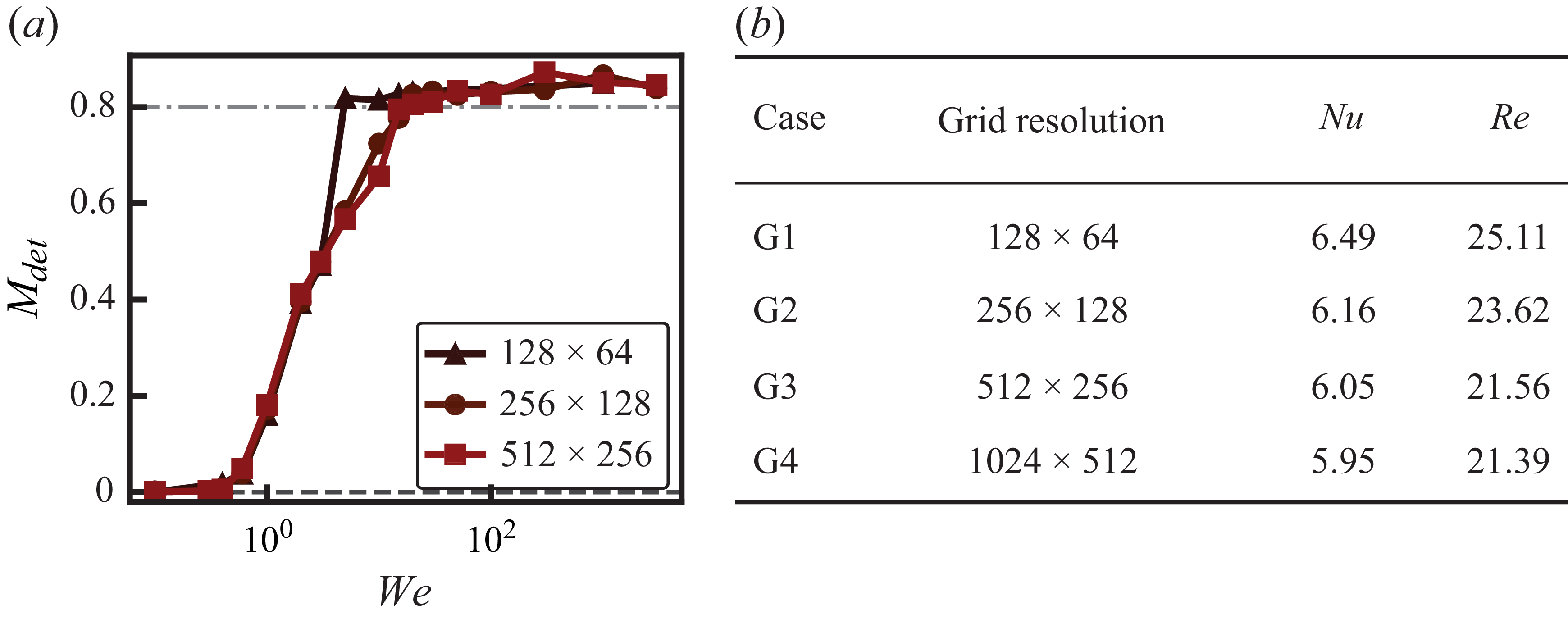
We assess grid dependence at
 $\alpha _1/\alpha _0=7$
using both the transition curve and the global transport statistics. Figure 9(a) shows that the
 $128\times 64$
grid predicts earlier detachment, whereas the
 $256\times 128$
and
 $512\times 256$
curves are closely aligned; their sampled detachment thresholds differ by one
 $\textit{We}$
interval. At
 $\textit{We}=1000$
, the
 $\textit{Nu}$
and
 $\textit{Re}$
values on the
 $512\times 256$
production grid are also close to those on the finest
 $1024\times 512$
grid (figure 9
b). The agreement in the state sequence, transition range and global transport statistics supports the production-grid resolution used here.
Grid-refinement tests at
 $\alpha _1/\alpha _0=7$
. (
 $a$
) Elevated dispersed-phase fraction
 $M_{\textit{det}}$
as a function of
 $\textit{We}$
on three grids; the horizontal reference levels
 $M_{\textit{det}}=0$
and
 $0.8$
denote the ideal layered limit and the approximately uniform vertical distribution expected after detachment, respectively. (
 $b$
) Time-averaged
 $\textit{Nu}$
and
 $\textit{Re}$
at
 $\textit{We}=1000$
on four grids.

Appendix C. Influence of the vibration frequency
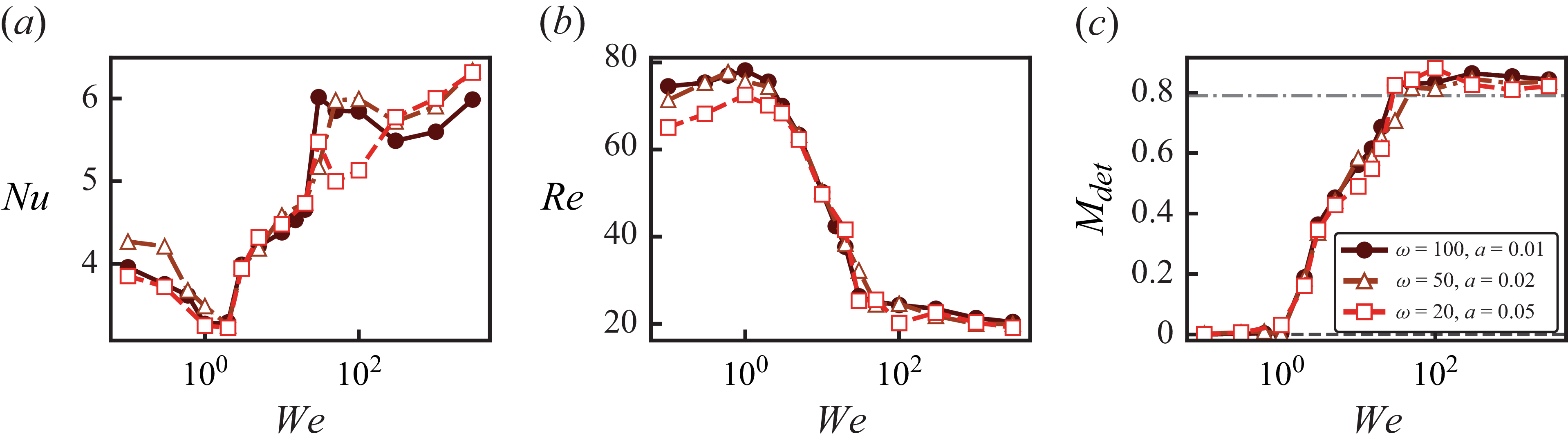
To assess the influence of vibration frequency at fixed forcing intensity, we compare Weber-number sweeps at
 $\textit{Ra}_{vib}=10^5$
and
 $\alpha _1/\alpha _0=5$
for
 $\omega =100$
, 50 and 20. The corresponding amplitudes are
 $a=0.01$
, 0.02 and 0.05, respectively, since
 $\omega =a^{-1}$
under the present scaling. The amplitude is therefore adjusted as the frequency is varied to maintain the same vibrational Rayleigh number.
Figure 10 shows quantitative differences in
 $\textit{Nu}$
and
 $\textit{Re}$
, particularly at low
 $\textit{We}$
and near droplet detachment, indicating that
 $\textit{Ra}_{vib}$
alone does not determine the transport response. Nevertheless, the
 $M_{\textit{det}}$
curves retain the progression from stratification through interfacial bulging to droplet dispersion, with transitions occurring over comparable Weber-number ranges. These results support the persistence of the state sequence over the tested frequencies, but the finite
 $\textit{We}$
sampling does not establish frequency-independent critical thresholds.
Influence of vibration frequency at fixed
 $\textit{Ra}_{vib}=10^5$
and
 $\alpha _1/\alpha _0=5$
. (
 $a$
) Nusselt number
 $\textit{Nu}$
, (
 $b$
) Reynolds number
 $\textit{Re}$
and (
 $c$
) elevated dispersed-phase fraction
 $M_{\textit{det}}$
as functions of
 $\textit{We}$
for
 $\omega =100$
, 50 and 20, corresponding to
 $a=0.01$
, 0.02 and 0.05, respectively.

Appendix D. Scaling estimate for the thermovibrational detachment force
This appendix summarises the scaling argument used to estimate the effective thermovibrational force responsible for droplet detachment. We first write the relevant estimates in dimensional form and then introduce the non-dimensional Weber number through the final force balance. The imposed horizontal vibration has a displacement scale
 $A$
and angular frequency
 $\varOmega$
, so that the acceleration scale is
 $A\varOmega ^2$
. In a thermally stratified fluid, the oscillatory inertial body-force density associated with thermal expansion has the scale
 \begin{equation} f_{{vib},\textit{inst}}^{*}\sim \rho _0 \alpha A\varOmega ^2 \Delta T . \end{equation}
For the two-phase system, the common part of this response gives a baseline thermovibrational driving. The additional driving relevant to interfacial deformation and detachment comes from the mismatch across the interface. Its instantaneous dimensional scale is
 \begin{equation} \Delta f_{{vib},\textit{inst}}^{*} \sim \rho _0(\alpha _1-\alpha _0)A\varOmega ^2\Delta T . \end{equation}
This contribution changes sign over a vibration period. The associated relative vibration velocity accumulated over one oscillation period is estimated as
 \begin{equation} U_{\textit{rel}}^{*} \sim \frac {\Delta f_{{vib},\textit{inst}}^{*}}{\rho _0\varOmega } \sim (\alpha _1-\alpha _0)A\varOmega \Delta T . \end{equation}
With the vibration velocity scale
 $U_v=\alpha _0 A\varOmega \Delta T$
, the same estimate can be written as
 \begin{equation} U_{\textit{rel}}^{*} \sim U_v\left (\frac {\alpha _1}{\alpha _0}-1\right )\!. \end{equation}
The first-order oscillatory velocity has zero mean over a vibration period. The leading non-zero averaged inertial contribution is therefore quadratic in the relative velocity. Using
 $H$
as the characteristic length of the lifted structure, the corresponding inertial acceleration scale is
 \begin{equation} a_{\textit{in}}^{*} \sim \frac {U_{\textit{rel}}^{*2}}{H} \sim \frac {U_v^2}{H} \left (\frac {\alpha _1}{\alpha _0}-1\right )^2 . \end{equation}
This inertial response gives an effective contrast-dependent force density of order
 $\rho _0a_{{in}}^{*}$
. For a dimensional lifted volume
 $V_d^{*}$
, the corresponding driving force has the scale
 \begin{equation} F_{\textit{contrast}}^{*} \sim \frac {\rho _0U_v^2}{H} \left (\frac {\alpha _1}{\alpha _0}-1\right )^2V_d^{*}, \end{equation}
where the order-one coefficient associated with this projection is introduced below in the complete force balance. The common thermovibrational response gives a baseline contribution with the same reference inertial-force scale,
 \begin{equation} F_{\textit{base}}^{*} \sim \frac {\rho _0U_v^2}{H}V_d^{*}, \end{equation}
where the order-one coefficient associated with this baseline response is introduced below in the complete force balance. The complete dimensional driving force may therefore be written as
 \begin{equation} F_{{vib}}^{*} \sim \frac {\rho _0U_v^2}{H} \left [ B+C\left (\frac {\alpha _1}{\alpha _0}-1\right )^2 \right ]V_d^{*} . \end{equation}
The first term is the baseline thermovibrational contribution, while the second term is the contrast-dependent inertial contribution. This complete form gives a finite threshold in the low-contrast limit through
 $B$
.
The variation of the detachment threshold with thermal-expansion contrast is governed by the contrast-dependent inertial contribution. Let
 $r=\alpha _1/\alpha _0$
. This contribution is of order
 $O[(r-1)^2]$
, whereas the baseline and lower-order contributions mainly provide weak offsets or prefactor corrections. In this contrast-dominated limit, the reduced dimensional driving force is
 \begin{equation} F_{{vib}}^{*} \sim \frac {\rho _0U_v^2}{H} \left (\frac {\alpha _1}{\alpha _0}-1\right )^2V_d^{*} . \end{equation}
The resisting force is the capillary force retaining the remaining neck,
 \begin{equation} F_{\sigma }^{*}\sim \sigma L_n^{*}, \end{equation}
where
 $L_n^{*}$
is the dimensional contact length of the neck. Balancing the dimensional driving and resisting forces gives
 \begin{equation} \frac {\rho _0U_v^2}{H} \left (\frac {\alpha _1}{\alpha _0}-1\right )^2V_d^{*} \sim \sigma L_n^{*} . \end{equation}
We now introduce the non-dimensional quantities
 $\textit{We}=\rho _0U_v^2H/\sigma$
,
 $L_n=L_n^{*}/H$
and
 $V_d=V_d^{*}/H^3$
. The force balance then becomes
 \begin{equation} \textit{We} \left (\frac {\alpha _1}{\alpha _0}-1\right )^2V_d \sim L_n, \end{equation}
and the corresponding droplet-detachment threshold is
 \begin{equation} \textit{We}_{c,\textit{det}} \sim \frac {L_n}{V_d} \left (\frac {\alpha _1}{\alpha _0}-1\right )^{-2}, \end{equation}
up to a prefactor. The comparison in figure 5(c) shows that the measured droplet-detachment thresholds are well captured by this reduced form, further supporting the simplification over the parameter range considered.

 a
 Nu/Nus
 We
 b
 We=20
 We=20
 c
 d
 c
 C=0.5

 a
 c
 a
 We=0.1
 b
 We=2
 c
 We=1000
 d
 f
 g
 Nu
 We
 α1/α0
 h
 Re
 We
 Ravib=105
 a=0.01

 a
 Trms
 b
 wrms
 α1/α0=4
 We=0.1
 We=15
 We=300
 z/H=−0.3

 a
 zs(x)=z0+ηcos(kmx)
 Δpvib
 Δpσ
 b
 Mdet
 We
 α1/α0
 Wec,bulging
 α1/α0=5
 Mdet
 z0
 c
 Wec,bulging
 α1/α0
 Wec,bulging
 α1/α0
 Wec,bulging∼(α1/α0−1)−2

 a
 Vd
 Ln
 b
 Vd
 Wec,det
 α1/α0
 ±10%
 Vd
 c
 Wec,det
 α1/α0
 Cf(α1/α0−1)−2
 Cf
 LnVd−1(α1/α0−1)−2
 Vd
 Ln

 a
 Nu
 b
 Re
 We/Wec,bulging
 α1/α0
 c
 Nu
 d
 Re
 We/Wec,det
 We/Wec,bulging=1
 a
 b
 We/Wec,det=1
 c
 d

 a
 (α1/α0,We)
 Mdet
 Wec,bulging∼(α1/α0−1)−2
 Wec,det∼(α1/α0−1)−2
 b
 a
 Ravib
 b
 Emass=|Vdisp(t)−Vdisp(0)|/Vdisp(0)
 c
 S/D
 (S/D)−3/2
 (S/D)−10/3

 α1/α0=7
 a
 Mdet
 We
 Mdet=0
 0.8
 b
 Nu
 Re
 We=1000
 Ravib=105
 α1/α0=5
 a
 Nu
 b
 Re
 c
 Mdet
 We
 ω=100
 a=0.01



