2.1. Feedback Effects

Although feedback effects are likely to be less important in trading than in macroeconomic decision making, i.e., when considering the effect of monetary policy, they can and do exist in trading by large financial corporations, and the preceding application can be readily adapted to show the additional issues that could arise when the possibility of feedbacks from d_t to x_t is recognized by the decision maker. For simplicity of exposition let s = 1 and suppose that such feedback only takes place through the effects of changes in trade positions on returns. Assume also that the change in the trade position decided at the end of period T is filled some time during the interval (T;T + 1], Δd_T+1 = d_T+1 − d_T = d_T* − d_T, or more generally d_t+1 = d_t* for all t. Under this setup a simple model of returns that allows for feedback is given by

where M_i,T denotes the return regression model assumed by the trader to hold at the end of period T. The coefficient ψ_i ≥ 0 measures the trader's perception of his market impact under M_i,T.⁴

Abstracting from VaR considerations, in this case we have

Under zero market impact, ψ_i = 0, this solution reduces to the standard mean-variance result, β_i′x_iT /φσ_iT². To implement d_T+1, the trader would need to estimate the parameters {ψ_i, β_i} and the return volatility, σ_iT². Because these parameters are specific to the model used by the trader they can, at best, be estimated for the particular model that had been used by the trader during the estimation period prior to date T. In reality, the trader might have used many different models in the past, and in that case historical observations on d_t,r_t, and x_t, t = T,T − 1,…, would not be relevant to the estimation of the parameters of model M_i,T. The problem arises more clearly if the trader in fact wishes to consider a counterfactual exercise with respect to any model, say, M_j,T, which has been used by him or her in the past. It is not clear how historical data could be used by the trader to estimate the market impact coefficient, ψ_j, under M_j,T. One way to get around this problem is by generating a sample that is consistent with the counterfactual policy. Such experiments can be costly, though, and are typically not available for econometric estimation purposes.

This application shows many choices that a decision maker will be faced with, even if the nature of the decision problem and the space of assets to be traded are taken as given. In what follows we consider some of these issues more generally and the type of solutions suggested in the literature for dealing with them.

3.1. Formulation and Selection of Models

For a given loss function and a time series of past measurements,

on the decision and state variables z_t = (d_t,x_t), the single most important task facing the decision maker at time T is the choice of the forecasting model,

. The real-time nature of the decision making process recognizes that the forecasting model and its parameters might need updating at the start of each decision period (say, prior to opening of markets). This could involve simple updating of parameters of a given model (keeping the specification of the model fixed) or updating the model by searching over a prespecified set of models or might even involve searching over new models including new variables/factors, functional forms, or dynamic specifications not considered as feasible or of potential usefulness prior to date T. These three levels of model updates can be viewed as “recursive estimation,” “recursive modeling,” and “innovative modeling,” respectively. Clearly, recursive modeling involves recursive estimation but not vice versa, and innovative modeling could encompass both recursive modeling and recursive estimation.

Selection of a model for use in decision making involves providing an answer to a counterfactual exercise, namely, a comparative analysis of the losses that would have been realized in the past under alternative specifications of the forecasting model (and hence the decision rules). Assume that

, the data generating process (DGP), is unknown and suppose that at time T the decision maker is faced with a set of forecasting models,

. Each model, M_i, is defined by the conditional probability density function of x_t defined over the estimation period t = T₀,T₀ + 1,…,T, (T₀ ≥ 1), and the forecasting period, t = T + 1, in terms of a k_i × 1 vector of unknown parameters, θ_i, assumed to lie in the compact parameter space, Θ_i:

Conditional on each model, M_i, being true it will be assumed that the true value of θ_i, which we denote by θ_i0, is fixed and remains constant across the estimation and prediction periods and lies in the interior of Θ_i.⁶

Phillips (1996) discusses the possibility that none of the models in

represents the true DGP in which case the best (local) approximation is being sought.

which depends on the unknown parameters of the selected forecasting model,

. To derive an operationally feasible decision rule, one would need to replace θ_i with a suitable estimate or eliminate such parameters by integrating them out with respect to their posterior distributions using Bayesian techniques. Under both approaches we have

where ψ_i(.) represents the vector of decision rules that depends on the loss function and its parameters, φ, the choice of the forecasting model, M_i, and the particular procedure used to deal with the unknown coefficients, θ_i.

Under M_i, the estimation of θ_i, or derivation of its posterior distribution, can be based on the joint likelihood function of z_t defined over the “observation window”: t = T₀,T₀ + 1,…,T:

where

is the conditional density of the decision variables assuming model M_i holds. In general, there are complicated restrictions linking the solutions to the decision and estimation problems. However, in the case of atomistic agents where the feedback effects of d_t on x_t can be ignored so that

the estimation and decision problems are decoupled, and estimation can be based on the likelihood of the state variables alone:

This in turn may require that the decision variables are constrained to lie in a restricted set so that their simulated values computed conditional on model M_i do not influence the state variables. In evaluation of trading strategies this requirement is usually met by restricting the trading positions to be sufficiently small or by inclusion of appropriate penalty terms in the loss function so that

, where

is a restricted subset of

.

4.1. Choice of Forecasting Model

Econometric modeling is often guided by existing economic theory although this will typically only be broadly suggestive of which state variables or functional form to use in the econometric model. To learn about these, the econometrician will therefore in practice undertake substantial specification searches across the set of potential models,

. The search for the “best” or an “average” model involves using the same set of realizations (historical data) many times over. The outcome could also depend crucially on the choice of the criterion function (likelihood or utility), the extent to which model complexity is penalized, and the particular model space over which the search is carried out. As a result the in-sample penalized performance of the model selected is not an unbiased estimator of the model's subsequent (out-of-sample) performance and can severely underestimate the true loss.

One way to deal with this problem is to assess the statistical significance of the best model in the context of the specification search that preceded it. This is the approach taken, e.g., by Sullivan, Timmermann, and White (2001), who bootstrap performance statistics to evaluate the significance of the best model drawn from a larger universe. This method provides a correction to the standard p-value that conditions on one model (as if it were prespecified) and therefore ignores the search that preceded it.

Automation can assist in reducing, but not eliminating, the effects of data snooping and pretest bias. Subjective opinions about specific variables and functional forms are likely to benefit significantly from hindsight as such opinions will be formed after gaining experience with different modeling strategies on an existing data set. Automated data-driven model selection procedures do, to some extent, take the choice of model out of the hand of the modeler, although it is more difficult to reduce hindsight in the choice of the model set,

, or in the innovative modeling stage, i.e., when choosing how to revise and modify

over time.

Clearly, the extent to which biases in subjective choices can be reduced depends on the dimensionality of

. If

only contains a few explanatory variables and functional forms that the modeler (with the benefit of hindsight) knows work well, then data snooping biases will not be reduced by much. Only if the data and model set are sufficiently large will the hindsight in the choice of a particular model be reduced.

4.2. Variable Selection

Let

denote the time-invariant universe of all possible prediction variables that could be considered in the econometric model, whereas N_xt is the number of regressors available at time t so

. The number of regressors, N_xt, is likely to grow at a faster rate than the sample size, T. At some point there will therefore be more regressors than time-series observations. However, most new variables will represent different measurements of a finite number of underlying economic factors such as output/activity, inflation, and interest rates.

Rather than searching over all possible combinations of predictor variables at random, a sensible approach is to first categorize variables and then choose one or a few variables from each category. Alternatively, regressors can be clustered in advance according to a simple algorithm that measures their correlation or by grouping them according to what they measure (e.g., interest rates, inflation measures). One possibility, considered, e.g., by Stock and Watson (2002), is to extract common factors and use the most important of these in forecasting.

4.3. Recursive Modeling

In Pesaran and Timmermann (1995, 2000) we proposed a recursive modeling approach that exemplifies many of the points mentioned thus far, including how to estimate μ_it in Section 2. Consider an N_xt × 1 column vector v_i with a string of N_xt ones or zeros, where a one in the jth row means that the jth regressor is included in the model whereas a zero in the jth row means that this regressor is excluded from the model. Then each possible model at time t can be identified by the N_xt-digit string of zeros and ones corresponding to the binary code of its number. Without loss of generality, consider forecasting the first element of X_t+1,Y_t+1 = e_1t′X_t+1 (where e_1t′ is an N_xt-vector with unity in the first position and zeros elsewhere) at time t + 1 by means of linear regressions

where X_τ,i is a vector of regressors obtained as a subset of the regressors in contention, X_τ, and M_i(τ) denotes the ith regression model at time τ. Notice that this gives a total of 2^N_xT possible models. When N_xT is large, a comprehensive (global) search is therefore not feasible, and the approach could be modified by using Monte Carlo chain, simulated annealing, genetic algorithms, or a method such as PcGets.

Conditional on M_i(τ), and given the observations Y_τ+1, X_τ,i, τ = 1,2,…, T − 1, the parameters of model M_i can be estimated by least squares. Denoting these estimates by

, we have

These ordinary least squares (OLS) estimates are fairly simple to compute and

could be used as an estimate of μ_iT in our finance example in Section 2. The choice of X_T,i to be used in forecasting of Y_T+1 can be based on a number of likelihood-based model selection criteria suggested in the literature, such as Akaike's information criterion (AIC), Schwarz's Bayesian information criterion (BIC), or the posterior information criterion (PIC) of Phillips and Ploberger (1994), which applies to both stationary and nonstationary data.

This approach can of course readily be generalized to allow for nonlinear effects through indicator type variables as in threshold autoregressive models, Markov switching, or more complicated nonlinear indicators. As argued by Phillips (1996) it can also be used to choose design parameters such as whether or not to impose a unit root, choice of cointegration rank, and deterministic trend degree, etc., in broad classes of models such as reduced rank regressions, vector autoregressions (VARs), or Bayesian VARs. Whether only linear models or more general models are considered depends on the relative cost of searching across and estimating nonlinear models and the evidence of misspecification among linear models.

4.4. Model Averaging

So far we have focused on approaches that aim to select a single “best” model. More generally, the model determination process can be considered as selecting a set of weights on each of the models under consideration,

. If a single model is used only one of these weights will be nonzero, but it is possible to assign nonzero weights to several models simultaneously, to constrain the weights to add up to one (which makes sense if the individual forecasts are unbiased), and to impose nonnegativity of the weights. For example, the forecasting model under Bayesian model averaging (BMA) is given by

where

is the posterior probability of model M_i that is obtained from the prior distributions, the model priors Pr(M_i), and the priors for the unknown parameters, Pr(θ_i|M_i), and the likelihood functions of the models under consideration. BMA treats the underlying models as random variables. Markov chain Monte Carlo model composition (MC³) algorithms have been used to compute posterior probabilities for these models. Alternatively, Bayesian model selection methods based on, e.g., the model with the highest posterior probability can be used. For a discussion of related points and references to recent studies, see Section 11.3 in Koop (2003).

Note that the BMA density forecast depends on the particular set of models under consideration at time T. Model innovation concerns the evolution of the model space,

, over time, t. Conditional on

, model specification uncertainty can be taken into account by integrating the predictive density across the full set of models, i.e., by computing a weighted average of the predictive densities of each model. The weights can reflect either the (relative) likelihood values, the posterior probabilities as in (23), or the relative penalized likelihood values using a penalty term such as in the Akaike or Schwarz information criteria. Even with such approaches, it is still an open question which penalty function will yield the best results when judged according to the metric established by the economic loss function, [ell ].

Model averaging is particularly attractive in situations such as that reported by Phillips (1995) where the forecasts from the individual models are found to be very different and hence subject to a high degree of uncertainty. In the context of the asset allocation problem reviewed in Section 2, averaging could also proceed over probability density forecasts with different specifications of the conditional volatility, Σ_it.

A second possibility is to apply (Bayesian) shrinkage methods to the parameters of an individual forecasting model (e.g., a VAR) or to the combination weights (cf. Litterman, 1986). This is particularly attractive in the case of models with many parameters.

A third possibility is to apply the “thick modeling” method developed by Granger and Jeon (2004), which takes averages over the full set of models, suitably truncated to avoid using models with measurably poor performance.¹⁰

4.5. Data Window

Model instability is a real possibility due to technological or institutional changes and policy shifts. How much data to use in the modeling stage depends on the nature of possible model instability and the timing of possible breaks. To test for model instability, the full information set,

, should always be used to the extent possible. Once more is known about the nature of any model instability, an informed decision can be taken on how much data to discard.

Many classes of estimators take the form of weighted least squares. Let X_τ,i be the τth observation of the ith subset of X-variables. Further, let ω_τT ∈ [0;1] be the weight on observation τ at time T. Then

This class of estimators encompasses as special cases

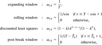
where win is some fixed, predetermined window length and

is the most recent breakpoint estimate obtained using data up to period T. Pesaran and Timmermann (2002) propose a reversed ordered (cumulative sum) CUSUM method that reverses the sequence of the data and tries to identify the most recent break in the data. This method is designed to answer how much historical data to use to estimate the parameters of a forecasting model. For example, when computing the conditional mean of stock returns, μ_it, one may choose only to use data after the oil price shocks of 1974 or after the stock market crash of 1987.

The expanding window method is efficient if the DGP is stationary and the model represents the true DGP. Discounted least squares is optimal in some settings with time-varying second moments, whereas the postbreak data window is optimal provided that a sufficiently large discrete break has occurred. This latter method is related to the approach of Phillips (1996) for discarding data prior to a certain time period based on the relative likelihood ratio of pairs of competing forecasting models.

4.6. Data Revisions and Measurement Errors

Macroeconomic variables in particular are often subject to important measurement errors and data revisions (cf. Croushore and Stark, 2001; Egginton, Pick, and Vahey, 2002). Where feasible, any real-time econometric model should make use of such data in all stages so as not to overstate the degree of predictability.

Financial variables such as interest rates and stock prices are typically not similarly affected by data revisions but may be subject to measurement errors—particularly when such data are fed into a computer in real time. To detect outliers that could lead to unreliable results, a filter could be designed that alerts users to aberrations more than a certain distance away from the standard range observed for a particular variable.

Other operational issues are likely to further constrain the econometric model. For a start, the time required to update a model forecast is constrained by real-time considerations. For example, if minute-by-minute trading is desired and the computation of a one-period forecast takes more than one minute, the forecast will be useless by the time it becomes available. The speed of the algorithm could therefore be an important consideration.

4.7. Cross-Validation

In view of the very large set of potential regressors in

, spurious relationships could well result from an extensive model specification search, and it is important to reduce the effects of data snooping. One strategy is to apply cross-validation techniques. This can be implemented by splitting the data set into a training sample [1; R] used to select an econometric model

and estimate its parameters to get a predictive density,

, and an evaluation sample [R + 1;T] used to evaluate the model. Because overparameterized models are likely to perform poorly in the cross-validation sample, this method can be viewed as an alternative way of penalizing for model complexity.

Cross-validation need not be based on the same metric as that used in the loss function. A range of alternative performance indicators—such as the percentage of correctly predicted signs or the Sharpe ratio in the case of a trading system—could also be used. This is important because the sampling distribution of the economic loss measure, [ell ](.), may be poorly behaved. Suppose, e.g., that the decision maker cares about the wealth generated by an automated trading system. Cumulated wealth, being the product of a sequence of returns over the trading period, is likely to have a sampling distribution with very large standard errors, so even a relatively long cross-validation sample could well lead to inconclusive results.

Cross-validation techniques have other limitations. The modeler is bound to have some knowledge of the basic characteristics of the historical data from R + 1 to T. This means that the cross-validation sample is not virgin data and could potentially bias the performance. As a case in point, an econometrician may have a data set on stock returns from 1985 to 2000 and use the first part of the data for model construction, whereas the latter half is used for cross-validation. Knowing that the last half included a sustained bull market could well bias the modeler to include “momentum” variables that would work very well in the cross-validation period although they would have little if any predictive power in the subsequent sample.

Furthermore, because the rules for the construction of the econometric system have to be “written in stone” and be in place at the outset of the cross-validation period, inevitably decision rules will be based on old data. This introduces a locality problem because it is likely that the econometric model would have worked better if more recent data could have been used to change the rules of the econometric system.

A final problem associated with cross-validation is that the statistical tests underlying the evaluation period are likely to have weak power and thus may not be very informative. One way to evaluate this loss in power is by quantifying the impact of the specification search leading to the “best” model using methods such as those adopted by Sullivan et al. (2001). Another strategy is to use stress-testing methods that either simulate or bootstrap from a model that captures salient features of the underlying data set and examines the performance of the model under a range of plausible scenarios.

4.8. Applications

Automated model selection is still a relatively recent tool, and not that much experience has yet been gained with it. Pesaran and Timmermann (1995, 2000), Phillips (1995), and Schiff and Phillips (2000) report the outcome of applications of automated model selection experiments for stock returns (portfolio allocation) and forecasts of Asia-Pacific (New Zealand) economic activity variables, respectively. Aiolfi and Favero (2002) use thick modeling to obtain recursive forecasts of asset returns. Coe, Pesaran, and Vahey (2003) provide an application of recursive modeling to the term structure of U.K. interest rates to see if econometric techniques could have been used to reduce the interest costs of managing public debt. These studies suggest that the automated procedures generally select parsimonious models whose simulated forecasting performances tend to be better than that provided by reasonable benchmarks such as forecasts based on random walk models or official forecasts (Schiff and Phillips, 2000).

These studies also point out that the best approximating model is time-varying. Phillips (1996) introduces the idea of the “lifetime” of an econometric model. Pesaran and Timmermann (2000) plot out a sequence of indicator variables tracking the inclusion or exclusion of a particular regressor in the forecasting model and find that some variables drop out after an initial inclusion period or get included in blocks in time.

Monte Carlo evidence reported by Hendry and Krolzig (2003) is also suggestive of the ability of automated modeling approaches to select key regressors at least in the context of linear models in a stationary environment.

Phillips (2003) proposes a powerful future application that would make econometric model determination software available to nonexpert users via the Web. Users choose a set of potentially relevant forecasting variables and may also provide their own data. The software then produces outputs such as graphs of forecasts surrounded by standard error bands. An extension of this idea is to link the forecasts with an objective function representing the user's attitude toward risk and an optimizer and solve for variables such as savings and portfolio choices.

5.1. Performance Monitoring

Once a model has been selected and cross-validated using data up to time T, it is reasonable to monitor its real-time performance at regular intervals, e.g., every h periods at time T + h, T + 2h, T + 3h,…,T + nh, where n is a positive integer. The monitoring frequency, h, should be a function of the degree of model instability observed in prior periods and also of the cost of the monitoring.

The initial model is naturally maintained provided that the economic or statistical loss does not exceed some predetermined value [ell ]_max:

where we recall that

is the predictive density conditional on model M_i and

If (25) is satisfied, then forecasts and decisions at time T + nh can be conditioned on M_i(T + nh). Alternatively, model rejection could be based on diagnostic tests that reflect the behavior of the forecast errors, e_t, an approach taken by PcGets. For example, one could monitor whether the forecast error exceeds a certain number (κ) of standard deviations of the forecasting model,

, although account also needs to be taken of possible fat tails in the distribution of the forecast errors.

5.2. Model Modification

If the criterion (25) fails to be satisfied, the model space could be expanded from

, say, where

so the new model and decision rule solve

Model modification may lead to the inclusion of an omitted factor deemed previously to be unimportant. One example of a dormant factor that came to life is oil prices during the seventies. Because oil prices varied far less prior to the 1970s, few econometric models included them, but this clearly changed subsequently.

Such modification could also be triggered automatically by some real-time monitoring system if there is evidence of a model breakdown. It is closely related to the framework for model determination proposed by Phillips (1996), which includes the possibility that the true probability measure underlying the DGP itself evolves over time due to technological or institutional shifts.

Quite independently of whether or not model performance is being considered, the parameter estimates,

, can be updated either every period (h = 1) or at regular intervals, again depending on the relative cost-benefit of such updates.

This process is very similar to the model evaluation stage used to cross-validate the econometric model over the in-sample period. It involves specifying a range of statistical performance measures that can be the basis for decisions on whether and how to modify the econometric model. As part of the monitoring, tests for structural breaks could also be undertaken. Unfortunately, existing breakpoint tests lack power against plausible (local) alternatives and in many cases do not provide precise information about the time of the break. Some breaks may, however, be large enough that they can be detected. Even when such tests indicate some form of instability they typically do not reveal the form of the instability, i.e., a breakdown in model parameters or the inclusion of new predictor variables.

5.3. Model Innovation

To avoid some of the same pitfalls involved in the initial model construction phase, the process of monitoring and modifying the econometric model in real time should be set out in advance prior to the beginning of the experiment. This amounts to specifying in advance how the model space is extended, i.e., setting out rules for constructing the sequence

. For example, one could specify rules for considering new families of models for the conditional mean, g*(X_τ,i;β_i), new predictive density models f*(X_τ,i;θ_i), or new classes of estimators,

. Thus, if the purpose is to study the efficient market hypothesis, one could introduce new forecasting models (e.g., cointegrating regressions, neural networks, or wavelets) only at the historical point when they were introduced. Finding that a particular econometric forecasting method could have been used to generate abnormal profits 10 years prior to its invention would not be of much interest. If there are changes to the set of feasible decision rules, one also needs to set out the sequence

.

Inevitably innovative modeling relies on the modeler's judgment, and so it is typically more difficult to automate this stage than, e.g., the selection of regressors from a prespecified universe. The role of automation in this stage is therefore still an open question.