1. Introduction
In tokamaks and stellarators, plasma instabilities limit
 ${\it\beta}$
(the ratio of the plasma pressure to the magnetic field pressure) to a level of several per cent. The related physics has been studied from the very beginning of fusion research, but still many issues remain unresolved [1, Reference Hender, Wesley, Bialek, Bondeson, Boozer, Buttery, Garofalo, Goodman, Granetz and Gribov2]. This field became a large science with dozens of publications appearing every month in journals and conference proceedings. In theory, it extends from the well-known general academic approaches [Reference Bernstein, Frieman, Kruskal and Kulsrud3–Reference Goedbloed and Poedts8] to elucidations of particular details [1, Reference Hender, Wesley, Bialek, Bondeson, Boozer, Buttery, Garofalo, Goodman, Granetz and Gribov2, Reference Mikhailovskii9]. Any attempt to review this area of knowledge is doomed to be fragmentary in both physics and references. Here, we discuss only several from the list of the most urgent problems of ITER [1, Reference Hender, Wesley, Bialek, Bondeson, Boozer, Buttery, Garofalo, Goodman, Granetz and Gribov2], which is currently the largest fusion project with a great impact on national programs worldwide. Briefly, wall stabilization is the central topic. Originally this was included in stability calculations by assuming that the vacuum vessel wall is an ideal conductor [Reference Bernstein, Frieman, Kruskal and Kulsrud3–Reference Mikhailovskii9]. Lately, attention has shifted to a more realistic analysis with a resistive wall, though the theory has been developed for very slow modes only.
The problem is known because of resistive wall mode (RWM) studies [1, Reference Hender, Wesley, Bialek, Bondeson, Boozer, Buttery, Garofalo, Goodman, Granetz and Gribov2, Reference Chu and Okabayashi10] with DIII-D tokamak as the main contributor of experimental results [Reference Chu and Okabayashi10–Reference Okabayashi, Matsunaga, Degrassie, Heidbrink, In, Liu, Reimerdes, Solomon, Strait and Takechi25]. Its solution is needed to reach the ITER [1, Reference Hender, Wesley, Bialek, Bondeson, Boozer, Buttery, Garofalo, Goodman, Granetz and Gribov2] and JT-60SA [Reference Kamada, Barabaschi, Ishida, Ide, Lackner, Fujita, Bolzonella, Suzuki, Matsunaga and Yoshida26, Reference Kamada, Barabaschi and Ishida27] goals because, if not stabilized, the RWMs can be a serious danger in advanced scenarios.
Among the DIII-D results, the most impressive, and still theoretically unexplained [Reference Hender, Wesley, Bialek, Bondeson, Boozer, Buttery, Garofalo, Goodman, Granetz and Gribov2, Reference Chu and Okabayashi10], is the rotational stabilization of RWMs [Reference Chu and Okabayashi10–Reference Okabayashi, Matsunaga, Degrassie, Heidbrink, In, Liu, Reimerdes, Solomon, Strait and Takechi25]. Its simple description is that stable operation significantly above the free-boundary ideal kink-mode
 ${\it\beta}$
limit is possible with a resistive wall and sufficient plasma rotation [Reference Strait, Bialek, Bogatu, Chance, Chu, Edgell, Garofalo, Jackson, Jensen and Johnson12]. This is illustrated by figure 1, showing a long pulse with high
 ${\it\beta}$
in the DIII-D. The demonstrated gain in
 ${\it\beta}$
makes such discharges an attractive option, but without a reliable predictive model, its extrapolation to ITER is problematic [1, Reference Hender, Wesley, Bialek, Bondeson, Boozer, Buttery, Garofalo, Goodman, Granetz and Gribov2, Reference Chu and Okabayashi10].
 ${\it\beta}$
significantly above the no-wall kink-mode stability limit is sustained for
 ${\sim}1.5$
s (blue) with a resistive wall and plasma rotation in DIII-D. A similar discharge (red) without sufficient rotation has a
 ${\it\beta}$
collapse soon after crossing the no-wall limit. (Figure 1 from [Reference Strait, Bialek, Bogatu, Chance, Chu, Edgell, Garofalo, Jackson, Jensen and Johnson12].)

The effect is robust and reproducible; it was also observed on the tokamaks JET [Reference Reimerdes, Hender, Sabbagh, Bialek, Chu, Garofalo, Gryaznevich, Howell, Jackson and La Haye21], NSTX [Reference Reimerdes, Hender, Sabbagh, Bialek, Chu, Garofalo, Gryaznevich, Howell, Jackson and La Haye21, Reference Sabbagh, Sontag, Bialek, Gates, Glasser, Menard, Zhu, Bell, Bell and Bondeson28, Reference Sontag, Sabbagh, Zhu, Menard, Bell, Bialek, Bell, Gates, Glasser and Leblanc29], JT-60U [Reference Takechi, Matsunaga, Aiba, Fujita, Ozeki, Koide, Sakamoto, Kurita, Isayama and Kamada30] and several other devices [Reference Chu and Okabayashi10]. However, it still remains a mystery [Reference Hender, Wesley, Bialek, Bondeson, Boozer, Buttery, Garofalo, Goodman, Granetz and Gribov2, Reference Chu and Okabayashi10]. Simple theoretical estimates show that, in the frame of ideal magnetohydrodynamics (MHD), the RWMs cannot be stabilized by the plasma rotation [Reference Zakharov and Putvinskii31–Reference Gimblett and Hastie34]. At the same time, there is a contrary opinion that, when the mode rotates fast enough, the resistive wall must behave like an ideal conductor and stabilize the mode [1, Reference Strait, Bialek, Bogatu, Chance, Chu, Edgell, Garofalo, Jackson, Jensen and Johnson12, Reference Okabayashi, Bialek, Bondeson, Chance, Chu, Garofalo, Hatcher, In, Jackson and Jayakumar17, Reference Strait, Garofalo, Jackson, Okabayashi, Reimerdes, Chu, Fitzpatrick, Groebner, In and La Haye23, Reference Haney and Freidberg35–Reference Igochine and Igochine40]. The experimental results, however, fall in between [Reference Chu and Okabayashi10–Reference Okabayashi, Matsunaga, Degrassie, Heidbrink, In, Liu, Reimerdes, Solomon, Strait and Takechi25, Reference Sabbagh, Sontag, Bialek, Gates, Glasser, Menard, Zhu, Bell, Bell and Bondeson28–Reference Takechi, Matsunaga, Aiba, Fujita, Ozeki, Koide, Sakamoto, Kurita, Isayama and Kamada30]. Also, the concepts of ‘fast enough’ rotation and transition from the resistive to superconducting reaction were not clarified in fusion theory.
Analysis of the RWM stability in the non-rotating plasma is often performed in the frame of ideal MHD [1, Reference Hender, Wesley, Bialek, Bondeson, Boozer, Buttery, Garofalo, Goodman, Granetz and Gribov2, Reference Chu and Okabayashi10–Reference Okabayashi, Matsunaga, Degrassie, Heidbrink, In, Liu, Reimerdes, Solomon, Strait and Takechi25, Reference Sabbagh, Sontag, Bialek, Gates, Glasser, Menard, Zhu, Bell, Bell and Bondeson28–Reference Takechi, Matsunaga, Aiba, Fujita, Ozeki, Koide, Sakamoto, Kurita, Isayama and Kamada30, Reference Haney and Freidberg35, Reference Chu, Chan, Chance, Edgell, Garofalo, Glasser, Guo, Humphreys, Jensen and Kim38, Reference Bialek, Boozer, Mauel and Navratil41–Reference Shiraishi, Aiba, Miyato and Yagi49]. The stabilizing effect of the rotation was shown in the models with dissipation [Reference Chu and Okabayashi10, Reference Chu, Bondeson, Chance, Liu, Garofalo, Glasser, La Haye, Lao and Navratil14, Reference La Haye, Bondeson, Chu, Garofalo, Liu, Navratil, Okabayashi, Reimerdes and Strait16, Reference Strait, Garofalo, Jackson, Okabayashi, Reimerdes, Chu, Fitzpatrick, Groebner, In and La Haye23, Reference Okabayashi, Matsunaga, Degrassie, Heidbrink, In, Liu, Reimerdes, Solomon, Strait and Takechi25, Reference Bondeson and Ward32, Reference Betti and Freidberg36, Reference Chu, Greene, Jensen, Miller, Bondeson, Johnson and Mauel50–Reference Wang, Guo and Liu64] that treated the resistive wall as a magneto-thin shell, disregarding the skin effect. This can be justified for slow evolution, but at faster rotations, the skin effect makes the wall reaction nonlinear, which affects the energy exchange and may essentially contribute to stabilization [Reference Pustovitov65–Reference Pustovitov67].
Incorporation of the skin effect in the wall into the RWM theory is a key point here. Mathematically, this requires a proper description of the plasma–wall electromagnetic interaction which is governed by the Maxwell equations and Ohm’s law for the resistive walls and can be coupled to the plasma by proper boundary conditions. In solving the outer task, we do not impose any constraint on the plasma model. This allows applications with only those minimal assumptions that are obviously needed for the coupling. For example, in some cases, it suffices to assume a linear plasma response to external perturbations instead of detailed specification of the plasma dynamics.
A schematic view of the perpendicular cross-section of the toroidal plasma separated from the wall by the vacuum gap. The plasma surface and inner surface of the wall are denoted as
 $S_{pl}$
and
 $S_{w}$
, respectively.

Theoretically, taking account of the skin effect is a step ahead of the traditional thin-wall approaches. Practically, this gives a tool for closer analysis of the events when the plasma generates a rotating perturbation.
The paper contains derivations based on the integral energy–torque balance, reductions of the general relations to simpler forms, stability analysis for the modes faster than conventional RWMs, estimates and discussion of theoretical and experimental results on RWMs and other phenomena where the resistive wall can affect the plasma stability.
2. Formulation of the problem
The configuration of interest is schematically shown in figure 2. A toroidal plasma is separated from the metal wall by a vacuum gap, and there is a vacuum behind the wall. In real tokamaks and stellarators, the walls are non-uniform with cuts, portholes, extensions, etc. This is carefully modelled in such codes as VALEN [Reference Bialek, Boozer, Mauel and Navratil41], STARWALL [Reference Strumberger, Merkel, Sempf and Günter68] or CarMa [Reference Albanese, Liu, Portone, Rubinacci and Villone69–Reference Villone, Liu, Paccagnella, Bolzonella and Rubinacci71]. Also, behind the first wall there can be other conductors. For example, the ITER design is better reproduced by a double wall [Reference Hender, Wesley, Bialek, Bondeson, Boozer, Buttery, Garofalo, Goodman, Granetz and Gribov2, Reference Gribov and Pustovitov72], and the JT-60SA vacuum vessel will also have a double-wall structure [Reference Kamada, Barabaschi and Ishida27]. Here such complications will not be discussed because, to begin with, we need a theory properly treating the nearest wall. The principal question here is whether or not the wall can only slow down the mode growth rate (compared to the ‘no-wall’ case) without other influences on the plasma stability. The latter viewpoint dominates in the RWM studies [1, Reference Hender, Wesley, Bialek, Bondeson, Boozer, Buttery, Garofalo, Goodman, Granetz and Gribov2, Reference Chu and Okabayashi10–Reference La Haye, Bondeson, Chu, Garofalo, Liu, Navratil, Okabayashi, Reimerdes and Strait16, Reference Strait18, Reference Garofalo20–Reference Okabayashi, Matsunaga, Degrassie, Heidbrink, In, Liu, Reimerdes, Solomon, Strait and Takechi25, Reference Sontag, Sabbagh, Zhu, Menard, Bell, Bialek, Bell, Gates, Glasser and Leblanc29–Reference Taylor, Connor, Gimblett, Wilson and Hastie37, Reference Igochine and Igochine40–Reference Chu and Ichiguchi46, Reference Chu, Greene, Jensen, Miller, Bondeson, Johnson and Mauel50, Reference Hu, Betti and Manickam52, Reference Berkery, Sabbagh, Reimerdes, Betti, Hu, Bell, Gerhardt, Manickam and Podestà57–Reference Wang, Guo and Liu64, Reference Strumberger, Merkel, Sempf and Günter68, Reference Chance, Chu, Okabayashi and Turnbull73]. It is supported by the theorem proved for a dissipationless plasma in the paper [Reference Pfirsch and Tasso74], which compels us to look for some dissipation inside the plasma [Reference Chu and Okabayashi10, Reference Chu, Bondeson, Chance, Liu, Garofalo, Glasser, La Haye, Lao and Navratil14, Reference La Haye, Bondeson, Chu, Garofalo, Liu, Navratil, Okabayashi, Reimerdes and Strait16, Reference Strait, Garofalo, Jackson, Okabayashi, Reimerdes, Chu, Fitzpatrick, Groebner, In and La Haye23, Reference Okabayashi, Matsunaga, Degrassie, Heidbrink, In, Liu, Reimerdes, Solomon, Strait and Takechi25, Reference Bondeson and Ward32, Reference Betti and Freidberg36, Reference Chu, Greene, Jensen, Miller, Bondeson, Johnson and Mauel50–Reference Wang, Guo and Liu64] as a reason for higher stability limits due to the rotational stabilization. Recently developed and quite intricate theories with kinetic models [Reference Okabayashi, Matsunaga, Degrassie, Heidbrink, In, Liu, Reimerdes, Solomon, Strait and Takechi25, Reference Liu, Chu, Chapman and Hender55–Reference Wang, Guo and Liu64] include the wall as a thin shell, completely disregarding the skin effect. Here, on the contrary, we mostly concentrate on the cases when this effect becomes noticeable.
Some estimates will be performed using the cylindrical model which is also convenient for introducing the main geometrical parameters. The wall minor radius and the wall thickness are characterized by typical dimensions
 $r_{w}$
and
 $d_{w}$
, as shown in figure 3. In tokamaks, stellarators and pinches, the walls are geometrically thin,
 $r_{w}\gg d_{w}$
. This, and the notion that the RWMs are slow modes [1, Reference Hender, Wesley, Bialek, Bondeson, Boozer, Buttery, Garofalo, Goodman, Granetz and Gribov2, Reference Chu and Okabayashi10–Reference Okabayashi, Matsunaga, Degrassie, Heidbrink, In, Liu, Reimerdes, Solomon, Strait and Takechi25, Reference Sontag, Sabbagh, Zhu, Menard, Bell, Bialek, Bell, Gates, Glasser and Leblanc29–Reference Chu and Ichiguchi46, Reference Shiraishi, Aiba, Miyato and Yagi49–Reference Wang, Guo and Liu64, Reference Strumberger, Merkel, Sempf and Günter68–Reference Chance, Chu, Okabayashi and Turnbull73, Reference Reimerdes, Bialek, Chance, Chu, Garofalo, Gohil, In, Jackson, Jayakumar and Jensen75], gave rise to so-called thin-wall approximation [Reference Hender, Wesley, Bialek, Bondeson, Boozer, Buttery, Garofalo, Goodman, Granetz and Gribov2, Reference Chu and Okabayashi10, Reference Garofalo, Jensen and Strait13, Reference Chu, Bondeson, Chance, Liu, Garofalo, Glasser, La Haye, Lao and Navratil14, Reference La Haye, Bondeson, Chu, Garofalo, Liu, Navratil, Okabayashi, Reimerdes and Strait16, Reference Okabayashi, Matsunaga, Degrassie, Heidbrink, In, Liu, Reimerdes, Solomon, Strait and Takechi25, Reference Haney and Freidberg35, Reference Bialek, Boozer, Mauel and Navratil41–Reference Chu, Chance, Glasser and Okabayashi43, Reference Chu and Ichiguchi46, Reference Shiraishi, Aiba, Miyato and Yagi49, Reference Ham, Gimblett and Hastie53–Reference Wang, Guo and Liu64, Reference Strumberger, Merkel, Sempf and Günter68, Reference Chance, Chu, Okabayashi and Turnbull73, Reference Bondeson, Liu, Gregoratto, Gribov and Pustovitov76–Reference Pustovitov79] in the RWM theory that assumes the normal component of the magnetic perturbation to be constant across the wall. This requires
 $s\gg d_{w}$
, where
 $s$
is the skin depth in the wall. We are going to compare the predictions of such models with the results obtained for faster modes when
 $s\ll d_{w}$
and the same wall becomes magnetically thick.
A cylindrical illustration of the task geometry. Plasma with radius
 $r_{pl}$
and a coaxial resistive wall with radius
 $r_{w}$
, uniform thickness
 $d_{w}$
and electrical conductivity
 ${\it\sigma}$
.

The real perturbed quantities will be represented as
 $$\begin{eqnarray}f(\boldsymbol{r},t)=\text{Re}\{f_{1}(\boldsymbol{r})\text{e}^{{\it\gamma}t}\}\end{eqnarray}$$
with complex growth rate
 $$\begin{eqnarray}{\it\gamma}={\it\gamma}_{R}+\text{i}{\it\gamma}_{I},\end{eqnarray}$$
where the real
 ${\it\gamma}_{R}$
and
 ${\it\gamma}_{I}=n{\it\omega}$
are the real growth rate and
 $n$
-fold frequency of the mode toroidal rotation and
 $n$
is the toroidal wavenumber. For estimates, when it is justified, we will use a simple cylindrical representation
 $$\begin{eqnarray}f_{1}=f_{1m}\exp \text{i}(m{\it\theta}-n{\it\zeta}),\end{eqnarray}$$
where
 ${\it\theta}$
and
 ${\it\zeta}$
are the poloidal and toroidal angles, and
 $f_{1m}$
is the amplitude.
The plasma stability is often analysed in the frame of the ideal MHD, which seems to be insufficient [Reference Hender, Wesley, Bialek, Bondeson, Boozer, Buttery, Garofalo, Goodman, Granetz and Gribov2, Reference Chu and Okabayashi10, Reference Chu, Bondeson, Chance, Liu, Garofalo, Glasser, La Haye, Lao and Navratil14–Reference Garofalo20, Reference Sontag, Sabbagh, Zhu, Menard, Bell, Bialek, Bell, Gates, Glasser and Leblanc29, Reference Liu, Chu, Chapman and Hender55] for treating the rotational stabilization of RWMs. The ideal MHD is, however, a well developed and powerful tool, and it would be only natural to use its potential for solving the RWM tasks. Here, we essentially lean on the fundamental MHD results [Reference Bernstein, Frieman, Kruskal and Kulsrud3–Reference Goedbloed and Poedts8] and introduce new elements in the manner of extension of the classical theory.
In a general case, the force balance for the plasma is described by
 $$\begin{eqnarray}{\it\rho}\frac{\text{d}\boldsymbol{v}}{\text{d}t}=-\boldsymbol{{\rm\nabla}}p+\boldsymbol{j}\times \boldsymbol{B}+\boldsymbol{N},\end{eqnarray}$$
where
 ${\it\rho}$
is the plasma mass density,
 $\text{d}/\text{d}t=\partial /\partial t+\boldsymbol{v}\boldsymbol{\cdot }\boldsymbol{{\rm\nabla}}$
,
 $\boldsymbol{v}$
is the plasma velocity,
 $t$
is the time,
 $p$
is the plasma pressure,
 $\boldsymbol{j}=\boldsymbol{{\rm\nabla}}\times \boldsymbol{B}$
is the current density,
 $\boldsymbol{B}$
is the magnetic field and
 $\boldsymbol{N}$
is the force responsible for the non-ideal effects, plasma rotation and/or anisotropy or some external force (
 $\boldsymbol{N}=0$
in the ideal MHD). Equation (2.4) is supplemented by the Maxwell equations that serve as a common basis uniting the regions with different properties (plasma, vacuum, metal). Finally, we have to add Ohm’s law for the wall. This system, with proper boundary conditions, is used for deriving the energy relations in §§ 3 and 4 and, later, for calculating the RWM growth rate. Hereinafter, the units are chosen so that the magnetic pressure is
 $\boldsymbol{B}^{2}/2$
(which should be replaced by
 $\boldsymbol{B}^{2}/(2{\it\mu}_{0})$
in SI units).
One possible improvement on the way to a better theory for RWMs could be the inclusion of more terms in
 $\boldsymbol{N}$
in (2.4). However, it cannot be an only strategy because the accuracy and adequacy of its solutions also depend on the boundary conditions. In § 5, these are discussed with examples of how they can affect the stability results. A general comparison theorem on the wall stabilization is presented in § 6.
The boundary conditions at the resistive wall depend on the perturbation penetration through the wall. Its calculation becomes an additional step if the ideal wall or magnetically-thin wall simplifications are waived, which is briefly discussed with emphasis on the case with a strong skin effect in § 7. This completes the mathematical background, and next follow the applications.
3. Energy relations in the inner region
A small displacement
 ${\bf\xi}$
from equilibrium is described by the equation
 $$\begin{eqnarray}{\it\rho}_{0}\frac{\partial ^{2}{\bf\xi}}{\partial t^{2}}=\boldsymbol{F}({\bf\xi})+{\it\delta}\boldsymbol{N}({\bf\xi})\end{eqnarray}$$
obtained by linearizing (2.4). Here
 ${\it\delta}\boldsymbol{N}$
represents the input from
 $\boldsymbol{N}-{\it\rho}(\boldsymbol{v}\boldsymbol{\cdot }\boldsymbol{{\rm\nabla}})\boldsymbol{v}$
,
 $$\begin{eqnarray}\boldsymbol{F}=-\boldsymbol{{\rm\nabla}}\tilde{p}+\boldsymbol{j}_{0}\times \boldsymbol{b}+\tilde{\boldsymbol{j}}\times \boldsymbol{B}_{0}\end{eqnarray}$$
is the standard MHD force operator with
 $\tilde{p}=p-p_{0}$
the pressure perturbation,
 $\boldsymbol{j}_{0}$
and
 $\boldsymbol{B}_{0}$
the equilibrium current density and magnetic field and
 $\tilde{\boldsymbol{j}}=\boldsymbol{{\rm\nabla}}\times \boldsymbol{b}$
with
 $\boldsymbol{b}$
a small perturbation:
 $$\begin{eqnarray}\boldsymbol{B}=\boldsymbol{B}_{0}+\boldsymbol{b}.\end{eqnarray}$$
In typical cases, the solution to (3.1) can be expressed through two eigenfunctions with
 $\sin$
,
 $\cos$
or
 $\exp$
dependence on time and angles. Then it is convenient to introduce the complex variables as in (2.1). Representing a real perturbation
 ${\bf\xi}$
in such a form, multiplying (3.1) by
 ${\bf\xi}^{\ast }$
(the complex conjugate) and integrating over the plasma volume
 $V_{pl}$
, one obtains
 $$\begin{eqnarray}{\it\delta}K+W_{p}+N=S_{p},\end{eqnarray}$$
where
 $N$
denotes a contribution from
 ${\it\delta}\boldsymbol{N}$
and other non-ideal effects such as, for example, plasma resistivity and non-adiabaticity,
 $$\begin{eqnarray}\displaystyle & \displaystyle {\it\delta}K\equiv \frac{1}{2}\int _{V_{pl}}{\it\rho}_{0}{\bf\xi}^{\ast }\frac{\partial ^{2}{\bf\xi}}{\partial t^{2}}\,\text{d}V, & \displaystyle\end{eqnarray}$$
 $$\begin{eqnarray}\displaystyle & \displaystyle W_{p}\equiv \frac{1}{2}\int _{V_{pl}}[|\boldsymbol{b}|^{2}+{\it\Gamma}p_{0}|\text{div}\,{\bf\xi}|^{2}+({\bf\xi}\boldsymbol{\cdot }\boldsymbol{{\rm\nabla}}p_{0})\text{div}\,{\bf\xi}^{\ast }-{\bf\xi}^{\ast }\boldsymbol{\cdot }(\boldsymbol{j}_{0}\times \boldsymbol{b})]\,\text{d}V, & \displaystyle\end{eqnarray}$$
 $$\begin{eqnarray}\displaystyle & \displaystyle S_{p}\equiv -\frac{1}{2}\oint _{S_{pl}}(\tilde{p}+\boldsymbol{b}_{i}\boldsymbol{\cdot }\boldsymbol{B}_{0i}){\bf\xi}^{\ast }\boldsymbol{\cdot }\text{d}\boldsymbol{S}, & \displaystyle\end{eqnarray}$$
 ${\it\Gamma}$
is the ratio of the specific heats,
 $S_{pl}$
is the plasma boundary and the subscript
 $i$
in (3.7) means the inner side of
 $S_{pl}$
. We do not show the details of the derivations because they can be found in [Reference Bernstein, Frieman, Kruskal and Kulsrud3–Reference Goedbloed and Poedts8] and other textbooks and papers on the energy principle. In particular, at
 $N=0$
, (3.4) corresponds to (2) in [Reference Chu, Chance, Glasser and Okabayashi43] where it was further reduced in the thin-wall approximation. In the standard ideal MHD model [Reference Bernstein, Frieman, Kruskal and Kulsrud3–Reference Goedbloed and Poedts8], expressions (3.6) and (3.7) are obtained from (3.1) and (3.2) with
 $\boldsymbol{b}=\boldsymbol{{\rm\nabla}}\times ({\bf\xi}\times \boldsymbol{B}_{0})$
,
 $\tilde{p}=-{\bf\xi}\boldsymbol{\cdot }\boldsymbol{{\rm\nabla}}p_{0}-{\it\gamma}p_{0}\,\text{div}\,{\bf\xi}$
and
 $\boldsymbol{B}_{0}\boldsymbol{\cdot }\text{d}\boldsymbol{S}_{pl}=0$
. Here, without these restrictions on
 $\boldsymbol{b}$
and
 $\tilde{p}$
, the difference from the static ideal MHD is represented by
 $N$
in (3.4).
In traditional stability theory [Reference Bernstein, Frieman, Kruskal and Kulsrud3–Reference Goedbloed and Poedts8], the last term on the right-hand side of (3.7) is transformed by using the force-balance equation at the plasma edge and the condition
 $$\begin{eqnarray}\boldsymbol{n}_{pl}\times (\boldsymbol{E}_{e}+\boldsymbol{v}\times \boldsymbol{B}_{e})=0\end{eqnarray}$$
following from the continuity of the tangential component of
 $\boldsymbol{E}$
at
 $S_{pl}$
(the subscript
 $e$
means its external side) under the ideal-plasma constraint
 $\boldsymbol{E}+\boldsymbol{v}\times \boldsymbol{B}=0$
. When the equilibrium velocity
 $\boldsymbol{v}_{0}$
is small at the plasma edge, with (3.8) one obtains
 $$\begin{eqnarray}\int _{S_{pl}}(\boldsymbol{b}_{e}\boldsymbol{\cdot }\boldsymbol{B}_{0e})\dot{{\bf\xi}}^{\ast }\boldsymbol{\cdot }\text{d}\boldsymbol{S}=\int _{S_{pl}}(\boldsymbol{E}_{e}^{\ast }\times \boldsymbol{b}_{e})\boldsymbol{\cdot }\text{d}\boldsymbol{S}.\end{eqnarray}$$
This looks similar to the last term in (3.7), but contains
 $\boldsymbol{B}_{0}$
and
 $\boldsymbol{b}$
at the outer side of
 $S_{pl}$
and
 $\dot{{\bf\xi}}^{\ast }\equiv \partial {\bf\xi}^{\ast }/\partial t$
which reduces to
 ${\it\gamma}^{\ast }{\bf\xi}^{\ast }$
if the time behaviour of the perturbations is described by
 $\exp ({\it\gamma}t)$
. This is an intermediate step in the standard ideal MHD where
 $\boldsymbol{E}$
is eliminated at once by further transformations, see [Reference Bernstein, Frieman, Kruskal and Kulsrud3–Reference Goedbloed and Poedts8]. Here we do not follow this tradition. Keeping the term with
 $\boldsymbol{E}$
in this form, and allowing for other physics than that implied by (3.8) and (3.9), we can cast (3.4) in the form
 $$\begin{eqnarray}{\it\delta}K+W_{p}+N+W_{s}=-\frac{1}{2{\it\gamma}^{\ast }}\int _{S_{pl}}(\boldsymbol{E}_{e}^{\ast }\times \boldsymbol{b}_{e})\boldsymbol{\cdot }\text{d}\boldsymbol{S},\end{eqnarray}$$
where
 $W_{s}$
is a surface integral such that
 $W_{s}+S_{p}$
gives the right-hand side of (3.10).
In the ideal MHD,
 $N=0$
and
 $W_{s}$
reduces to standard expressions (at
 $\boldsymbol{v}_{0}=0$
, see the last integral in (2.7) in [Reference Kadomtsev and Leontovich4], (8.97b) in [Reference Freidberg5] or (8.47) in [Reference Miyamoto6]). Here, we mention the ideal MHD as a reference model and include its results as a part of our more general approach for a potentially non-ideal plasma.
In any case, the plasma properties are contained on the left-hand side of (3.10), while the right-hand side remains the same for any plasma model. The latter property makes (3.10) a convenient starting point for stability analysis, especially when the influence of the outer area should be investigated.
It follows from the Maxwell equations
 $$\begin{eqnarray}\displaystyle & \displaystyle \boldsymbol{{\rm\nabla}}\times \boldsymbol{E}=-\partial \boldsymbol{b}/\partial t, & \displaystyle\end{eqnarray}$$
 $$\begin{eqnarray}\displaystyle & \displaystyle \boldsymbol{{\rm\nabla}}\times \boldsymbol{b}=\tilde{\boldsymbol{j}} & \displaystyle\end{eqnarray}$$
that
 $$\begin{eqnarray}\boldsymbol{{\rm\nabla}}\boldsymbol{\cdot }(\boldsymbol{E}^{\ast }\times \boldsymbol{b})=-\tilde{\boldsymbol{j}}\boldsymbol{\cdot }\boldsymbol{E}^{\ast }-{\it\gamma}^{\ast }|\boldsymbol{b}|^{2}.\end{eqnarray}$$
With its integral consequence, (3.10) is transformed into
 $$\begin{eqnarray}{\it\delta}K+W_{p}+N+W_{s}+W_{g}=-F,\end{eqnarray}$$
where
 $W_{g}$
represents the magnetic energy of the perturbation in the plasma–wall vacuum gap,
 $$\begin{eqnarray}W_{g}=\int _{gap}\frac{|\boldsymbol{b}|^{2}}{2}\,\text{d}V,\end{eqnarray}$$
and
 $F$
describes the Poynting vector flux through the wall:
 $$\begin{eqnarray}F\equiv \frac{1}{2{\it\gamma}^{\ast }}\int _{wall-}(\boldsymbol{E}^{\ast }\times \boldsymbol{b})\boldsymbol{\cdot }\text{d}\boldsymbol{S}_{w}.\end{eqnarray}$$
Here ‘
 $wall-$
’ denotes the inner surface of the vacuum chamber,
 $S_{w}$
, to distinguish it further from the outer surface of the wall ‘
 $wall+$
’,
 $\text{d}\boldsymbol{S}_{w}=\boldsymbol{n}_{w}\,\text{d}S_{w}$
is the oriented element of the area of
 $S_{w}$
and
 $\boldsymbol{n}_{w}$
is the outward unit normal to
 $S_{w}$
.
4. Energy relations in the outer region
In classical stability theory [Reference Bernstein, Frieman, Kruskal and Kulsrud3–Reference Goedbloed and Poedts8], the wall is assumed ideal. This makes
 $F=0$
in (3.14). Moving the wall outwards and reducing its effect on the plasma, we arrive at the ‘no wall’ limit with the same
 $F=0$
, but with integration in (3.15) extended to infinity.
The condition
 $F=0$
strictly isolates the plasma from the external world. With a resistive wall, this isolation is broken. Then
 $F\neq 0$
, which is an essentially new element compared to [Reference Bernstein, Frieman, Kruskal and Kulsrud3–Reference Goedbloed and Poedts8]. We already know that it can strongly affect the solution of (3.14) converting the ideal MHD modes in the RWMs.
The studies of RWMs are ultimately aimed at developing a strategy allowing stable operation in the region where the RWMs are potentially unstable. The experiments show that this requires either plasma rotation or feedback control or both [Reference Hender, Wesley, Bialek, Bondeson, Boozer, Buttery, Garofalo, Goodman, Granetz and Gribov2, Reference Chu and Okabayashi10, Reference Turnbull, Brennan, Chu, Lao and Snyder19, Reference Garofalo20, Reference Sontag, Sabbagh, Zhu, Menard, Bell, Bialek, Bell, Gates, Glasser and Leblanc29]. In all cases, a reliable description of the ‘open loop’ system is needed as a basis for analysis. This means a correct calculation of the plasma interaction with the passive elements, which are simply called ‘wall’.
The interaction explicitly enters through
 $F$
, but also modifies
 $W_{g}$
in (3.14). The flux
 $F$
can be either prescribed by the boundary conditions at
 $S_{w}$
or found from the energy balance obtained by integrating the Poynting theorem (3.13) over the space behind the toroidal surface
 $S_{w}$
. In typical models of real tokamaks or stellarators [1, Reference Hender, Wesley, Bialek, Bondeson, Boozer, Buttery, Garofalo, Goodman, Granetz and Gribov2, Reference Chu and Okabayashi10, Reference Strait, Bialek, Bogatu, Chance, Chu, Edgell, Garofalo, Jackson, Jensen and Johnson12–Reference Chu, Bondeson, Chance, Liu, Garofalo, Glasser, La Haye, Lao and Navratil14, Reference Bondeson and Ward32–Reference Chu and Ichiguchi46, Reference Shiraishi, Aiba, Miyato and Yagi49–Reference Pustovitov79] this means integration over the wall and the external vacuum region. Then the result is
 $$\begin{eqnarray}F=D_{w}+W_{w}+W_{w+}\end{eqnarray}$$
with
 $D_{w}$
representing the resistive dissipation in the wall,
 $$\begin{eqnarray}D_{w}\equiv \frac{1}{2{\it\gamma}^{\ast }}\int _{wall}\tilde{\boldsymbol{j}}\boldsymbol{\cdot }\boldsymbol{E}^{\ast }\,\text{d}V=\frac{1}{2{\it\gamma}^{\ast }}\int _{wall}{\it\sigma}|\boldsymbol{E}|^{2}\,\text{d}V,\end{eqnarray}$$
where Ohm’s law in the form
 $\tilde{\boldsymbol{j}}={\it\sigma}\boldsymbol{E}$
is used for the wall, and
 $$\begin{eqnarray}W_{w}=\int _{wall}\frac{|\boldsymbol{b}|^{2}}{2}\,\text{d}V,\quad W_{w+}=\int _{wall+}\frac{|\boldsymbol{b}|^{2}}{2}\,\text{d}V,\end{eqnarray}$$
represent the magnetic energies in the wall and in the vacuum region behind the wall, respectively. In a more general case with some sources of
 $\boldsymbol{b}$
behind
 $S_{w+}$
(correction coils or passive elements), a proper additional source term should be added in (4.1).
With
 $\boldsymbol{b}=\boldsymbol{{\rm\nabla}}{\it\varphi}$
in a vacuum we have
 $$\begin{eqnarray}W_{w+}=-\frac{1}{2}\oint _{wall+}{\it\varphi}_{+}\boldsymbol{b}_{+}^{\ast }\boldsymbol{\cdot }\text{d}\boldsymbol{S}_{w},\end{eqnarray}$$
where the integration is performed over the outer side of the wall.
The flux
 $F$
can be similarly expressed as
 $$\begin{eqnarray}F=-\frac{1}{2}\oint _{wall-}{\it\varphi}_{-}\boldsymbol{b}_{-}^{\ast }\boldsymbol{\cdot }\text{d}\boldsymbol{S}_{w},\end{eqnarray}$$
but with integration over the inner side. The latter equality is obtained from (3.16) by using the identity
 $$\begin{eqnarray}\boldsymbol{E}^{\ast }\times \boldsymbol{b}=\boldsymbol{E}^{\ast }\times \boldsymbol{{\rm\nabla}}{\it\varphi}=-\boldsymbol{{\rm\nabla}}\times ({\it\varphi}\boldsymbol{E}^{\ast })+{\it\varphi}\boldsymbol{{\rm\nabla}}\times \boldsymbol{E}^{\ast }.\end{eqnarray}$$
The potentials and fields are different in (4.4) and (4.5) because of the currents in the wall which also determine the magnitude of the dissipation term
 $D_{w}$
. It follows from (4.2) that
 $$\begin{eqnarray}D_{w}={\it\gamma}{\it\tau}_{w}D_{0},\end{eqnarray}$$
with
 $D_{0}$
a function of
 $\boldsymbol{E}/{\it\gamma}$
only, and
 $$\begin{eqnarray}{\it\tau}_{w}\equiv {\it\sigma}_{0}r_{w}d_{w}.\end{eqnarray}$$
This constant (often called the wall time [Reference Chu and Okabayashi10, Reference Reimerdes, Hender, Sabbagh, Bialek, Chu, Garofalo, Gryaznevich, Howell, Jackson and La Haye21, Reference Chu and Ichiguchi46]) naturally appears in the thin-wall cylindrical models with
 ${\it\sigma}={\it\sigma}_{0}=\text{const.}$
, which will be used to derive estimates later. In such models with a uniform wall, the parameters
 ${\it\sigma}_{0}$
,
 $r_{w}$
and
 $d_{w}$
have clear meaning, but here they should be considered as ‘average’ or ‘fitting’ values so that (4.8) does not impose any restriction on the wall.
In (4.7),
 $D_{0}$
is a positive real quantity proportional to the volume integral in (4.2). If
 ${\it\sigma}|\boldsymbol{E}|^{2}$
could be constant across the wall (the key assumption in the thin-wall models),
 $D_{0}$
would reduce to the surface integral
 $$\begin{eqnarray}D_{0}^{sh}\equiv \frac{V_{w}}{2{\it\tau}_{w}}\frac{\langle {\it\sigma}|\boldsymbol{E}_{-}|^{2}\rangle }{|{\it\gamma}|^{2}}=\frac{S_{w}}{2r_{w}}\frac{\langle |\boldsymbol{E}_{-}|^{2}{\it\sigma}/{\it\sigma}_{0}\rangle }{|{\it\gamma}|^{2}}\end{eqnarray}$$
with
 $V_{w}=S_{w}d_{w}$
the wall volume,
 $\boldsymbol{E}_{-}$
the electric field at the inner side of the wall and the brackets denoting averaging over
 $S_{w}$
.
This is actually an upper estimate for
 $D_{0}$
. In fact,
 $$\begin{eqnarray}D_{0}={\it\alpha}D_{0}^{sh}\end{eqnarray}$$
with
 ${\it\alpha}\leqslant 1$
because of the radial decline of
 $\boldsymbol{E}$
in the wall:
 $$\begin{eqnarray}{\it\alpha}\equiv \frac{D_{w}}{{\it\gamma}{\it\tau}_{w}D_{0}^{sh}}=\int _{wall}\frac{{\it\sigma}|\boldsymbol{E}|^{2}}{\langle {\it\sigma}|\boldsymbol{E}_{-}|^{2}\rangle }\frac{\text{d}V}{V_{w}}.\end{eqnarray}$$
To express
 $D_{0}^{sh}$
and
 ${\it\alpha}$
in terms of the magnetic quantities, like those in (4.4) and (4.5), we have to solve (3.11). The task is simplified if the wall is geometrically thin. Then with
 $\tilde{\boldsymbol{j}}={\it\sigma}\boldsymbol{E}$
we need only the tangential component of
 $\boldsymbol{E}$
described by
 $$\begin{eqnarray}|\boldsymbol{{\rm\nabla}}a|\frac{\partial }{\partial t}\boldsymbol{b}\boldsymbol{\cdot }\boldsymbol{n}=\boldsymbol{{\rm\nabla}}\boldsymbol{\cdot }(\boldsymbol{{\rm\nabla}}a\times \boldsymbol{E}),\end{eqnarray}$$
which is a consequence of (3.11). Here
 $a(\boldsymbol{r})=\text{const.}$
is some parameterization of the family of the nested toroidal surfaces with
 $a=a_{w}$
and
 $a=a_{w}+d_{w}|\boldsymbol{{\rm\nabla}}a|$
representing the inner and outer sides of the wall (
 $S_{w}$
and
 $S_{w+}$
), respectively. The operator on the right-hand side of (4.12) is two-dimensional and can be easily inverted, providing us with
 $\boldsymbol{E}$
and
 $D_{0}$
as functions of
 $\boldsymbol{b}\boldsymbol{\cdot }\boldsymbol{n}$
.
The remaining quantity in (4.1),
 $W_{w}$
, is small compared to
 $W_{w+}$
if the wall is thin and penetration of
 $\boldsymbol{b}$
through the wall is good. These two conditions (with
 $\boldsymbol{b}\boldsymbol{\cdot }\boldsymbol{n}$
the same at the inner and outer sides of the wall) constitute the basis of the thin-wall models [Reference Hender, Wesley, Bialek, Bondeson, Boozer, Buttery, Garofalo, Goodman, Granetz and Gribov2, Reference Chu and Okabayashi10, Reference Garofalo, Jensen and Strait13, Reference Chu, Bondeson, Chance, Liu, Garofalo, Glasser, La Haye, Lao and Navratil14, Reference La Haye, Bondeson, Chu, Garofalo, Liu, Navratil, Okabayashi, Reimerdes and Strait16, Reference Okabayashi, Matsunaga, Degrassie, Heidbrink, In, Liu, Reimerdes, Solomon, Strait and Takechi25, Reference Haney and Freidberg35, Reference Bialek, Boozer, Mauel and Navratil41–Reference Chu, Chance, Glasser and Okabayashi43, Reference Chu and Ichiguchi46, Reference Shiraishi, Aiba, Miyato and Yagi49, Reference Ham, Gimblett and Hastie53–Reference Wang, Guo and Liu64, Reference Strumberger, Merkel, Sempf and Günter68, Reference Chance, Chu, Okabayashi and Turnbull73, Reference Bondeson, Liu, Gregoratto, Gribov and Pustovitov76–Reference Pustovitov79]. Then
 $$\begin{eqnarray}W_{w}=\int _{wall}\frac{|\boldsymbol{b}|^{2}}{2}\,\text{d}V<\frac{\max |\boldsymbol{b}|^{2}}{2}V_{w},\end{eqnarray}$$
and
 $W_{w}/W_{w+}\sim d_{w}/r_{w}\ll 1$
for the kink-like perturbations such as in (2.3).
Disregard of
 $W_{w}$
in favour of
 $W_{w+}$
is considered natural in the thin-wall models [Reference Chu and Okabayashi10, Reference Haney and Freidberg35, Reference Chu, Chance, Glasser and Okabayashi43, Reference Chu and Ichiguchi46]. However, it can be justified at
 $s\gg d_{w}$
only. Outside this rather narrow range, the skin effect inhibits the amplitude of
 $\boldsymbol{b}$
in the wall, so that finally we can expect the opposite
 $W_{w}/W_{w+}\gg 1$
at
 $0<s\ll d_{w}$
[Reference Pustovitov80, Reference Pustovitov81]. Below, both cases will be considered.
5. Boundary conditions
Two equations, (3.14) and (4.1), represent two parts of the system divided by
 $S_{w}$
. These equations could be used separately if the boundary conditions were properly prescribed at
 $S_{w}$
.
These conditions, needed to calculate
 $W_{g}$
and
 $F$
in (3.14), essentially affect the results of the stability analysis. This can be illustrated by the difference between
 ${\it\beta}_{N}^{wall}$
and
 ${\it\beta}_{N}^{\mathit{no\,wall}}$
, the stability limits for the same configuration computed, respectively, with ideal wall and without wall, in terms of the frequently used parameter
 $$\begin{eqnarray}{\it\beta}_{N}={\it\beta}~(\%)\frac{a~(\text{m})~B~(\text{T})}{I~(\text{MA})},\end{eqnarray}$$
where
 $a$
is the minor radius of the plasma,
 $B$
is the magnetic field and
 $I$
is the net current in the plasma. The representative examples are
 ${\it\beta}_{N}^{wall}=3.5{-}4$
and
 ${\it\beta}_{N}^{\mathit{no\,wall}}=2{-}2.5$
in ITER [Reference Hender, Wesley, Bialek, Bondeson, Boozer, Buttery, Garofalo, Goodman, Granetz and Gribov2],
 ${\it\beta}_{N}^{wall}=3.3$
and
 ${\it\beta}_{N}^{\mathit{no\,wall}}=1.8{-}2.2$
in the DIII-D tokamak [Reference Strait, Bialek, Bogatu, Chance, Chu, Edgell, Garofalo, Jackson, Jensen and Johnson12],
 ${\it\beta}_{N}^{wall}=4.3$
and
 ${\it\beta}_{N}^{\mathit{no\,wall}}=2$
in JT-60SA [Reference Kamada, Barabaschi, Ishida, Ide, Lackner, Fujita, Bolzonella, Suzuki, Matsunaga and Yoshida26] and
 ${\it\beta}_{N}^{wall}=5$
with
 ${\it\beta}_{N}^{\mathit{no\,wall}}=2.5$
in KSTAR [Reference Katsuro-Hopkins, Sabbagh, Bialek, Park, Bak, Chung, Hahn, Kim, Kwon and Lee82]. For more data and details see table II in [Reference Reimerdes, Hender, Sabbagh, Bialek, Chu, Garofalo, Gryaznevich, Howell, Jackson and La Haye21], figures 3 and 4 in [Reference Manickam, Chance, Jardin, Kessel, Monticello, Pomphrey, Reiman, Wang and Zakharov83] and discussion in [Reference Pustovitov65].
The ideal-wall models require
 $\boldsymbol{b}\boldsymbol{\cdot }\boldsymbol{n}_{w}=0$
. In the stability theory, this was usually introduced as
 $\boldsymbol{n}_{w}\times \boldsymbol{E}=0$
without alternatives [Reference Bernstein, Frieman, Kruskal and Kulsrud3, Reference Kadomtsev and Leontovich4, Reference Miyamoto6–Reference Goedbloed and Poedts8], though in [Reference Freidberg5] it was noted that, in some cases, the wall resistivity should be taken into account.
An ideal wall means no penetration of the perturbation through
 $S_{w}$
. If, on the contrary, the penetration is perfect, so that
 $\boldsymbol{b}\boldsymbol{\cdot }\boldsymbol{n}_{w}\neq 0$
is the same at the both sides of the wall, we have the so-called thin-wall approximation, the dominant approach in the existing RWM theory. In practice, the walls are geometrically thin (with a thickness
 $d_{w}$
much smaller than the minor radius
 $r_{w}$
), but for constant
 $\boldsymbol{b}\boldsymbol{\cdot }\boldsymbol{n}_{w}$
across the wall we need
 $s/d_{w}\gg 1$
, where
 $s$
is the skin depth. This allows slow modes only. The ideal-wall assumption corresponds to the opposite limit
 $s/d_{w}\rightarrow 0$
. The intermediate range around
 $s/d_{w}=1$
remains basically unexplored, which prompts us to fill this gap in theory.
In a general case, the normal component of
 $\boldsymbol{b}$
is not zero at
 $S_{w}$
and varies with distance across the wall so that
 $\boldsymbol{b}\boldsymbol{\cdot }\boldsymbol{n}_{w}$
is different at
 $S_{w}$
and
 $S_{w+}$
. Then a self-consistent prescription of
 $\boldsymbol{b}$
at the inner side of the wall depends on the
 $\boldsymbol{b}(\boldsymbol{r})$
behaviour in and behind the wall through the natural boundary conditions
 $$\begin{eqnarray}[[\boldsymbol{n}\boldsymbol{\cdot }\boldsymbol{b}]]=0,\quad [[\boldsymbol{n}\times \boldsymbol{b}/{\it\mu}]]=0\end{eqnarray}$$
at the wall–vacuum interfaces. Here the brackets
 $[[\cdots ]]$
mean the jump across the surface and
 ${\it\mu}$
is the magnetic permeability. In the RWM theory, usually ferromagnetic effects are disregarded, which is justified by analytical and numerical analysis [Reference Pustovitov84, Reference Pustovitov and Villone85] for slow modes. The situation is different for fast modes (at
 $s<d_{w}$
) [Reference Pustovitov and Yanovskiy86], which can be expected in future experiments in the JT-60SA tokamak [Reference Kamada, Barabaschi, Ishida, Ide, Lackner, Fujita, Bolzonella, Suzuki, Matsunaga and Yoshida26] and, possibly in experiments with a movable ferromagnetic wall in the HBT-EP tokamak [Reference Levesque, Hughes, Bialek, Byrne, Mauel, Navratil, Peng, Rhodes and Stoafer87]. However, more often the results obtained with
 ${\it\mu}=1$
are good enough and can be easily extended to the area with
 ${\it\mu}\neq 1$
[Reference Pustovitov and Yanovskiy86]. This is why
 ${\it\mu}=1$
is assumed in what follows.
With (5.2), calculation of
 $\boldsymbol{b}(\boldsymbol{r})$
in the wall becomes a part of the problem. In the earlier plasma stability theory, this task was avoided by assuming the wall to be ideal. Later, it was addressed in the most simple thin-wall formulation. These approaches are well developed, so more attention will be focused here on the intermediate case with a magnetically thick resistive wall.
6. Wall stabilization in terms of
 $W_{g}$

The benefits of the ideal wall stabilization in several tokamaks are explicitly demonstrated in the previous section. In reality, the walls are not perfect conductors and can produce only a partial stabilizing effect compared to the ideal case. Even this seems attractive for the success of a steady-state tokamak reactor [1]. Being an issue of particular importance for ITER, it was discussed in detail in [1, Reference Hender, Wesley, Bialek, Bondeson, Boozer, Buttery, Garofalo, Goodman, Granetz and Gribov2]. A nice review of the problem was recently given in [Reference Chu and Okabayashi10]. Here we mostly concentrate on the relevant theoretical aspects with more emphasis on yet unexplored areas.
When (3.14) is applied to the system with an ideal wall, it reduces to
 $$\begin{eqnarray}{\it\gamma}^{2}K_{0}=-(W_{p}+N+W_{s})-W_{g}\end{eqnarray}$$
with
 $$\begin{eqnarray}K_{0}\equiv \frac{1}{2}\int _{V_{pl}}{\it\rho}_{0}|{\bf\xi}|^{2}\,\text{d}V.\end{eqnarray}$$
In the static ideal MHD, (6.1) is further simplified, its right-hand side becomes real [Reference Bernstein, Frieman, Kruskal and Kulsrud3–Reference Goedbloed and Poedts8] with quantities containing
 ${\it\gamma}$
only through
 $\exp ({\it\gamma}t)$
dependence of
 ${\bf\xi}$
and
 $\boldsymbol{b}$
. It is clear that both
 $K_{0}$
and
 $W_{g}$
are positive, which means that the term
 $W_{g}$
is always stabilizing. At given plasma parameters, its contribution to (6.1) depends on the wall shape and location.
Precise evaluation of
 $W_{g}$
requires a knowledge of
 $\boldsymbol{b}(\boldsymbol{r})$
in the plasma–wall gap, but useful comparisons can be made in a general form using the property that
 $\boldsymbol{b}(\boldsymbol{r})$
in this vacuum region is determined by the normal component of
 $\boldsymbol{b}$
at the boundary. This includes the wall, where
 $\boldsymbol{b}\boldsymbol{\cdot }\boldsymbol{n}_{w}=0$
if it acts as an ideal conductor, and the plasma boundary
 $S_{pl}$
.
Consider two cases with the same plasma and the same
 $\boldsymbol{b}\boldsymbol{\cdot }\boldsymbol{n}_{pl}$
at
 $S_{pl}$
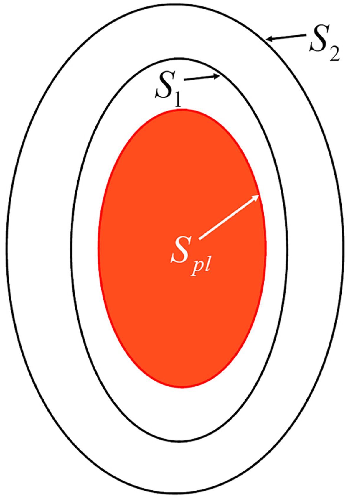
, but with different ideal walls, as schematically shown in figure 4. Then we have two toroidal vacuum regions, 1 (smaller) bounded by
 $S_{1}$
and 2 (larger) bounded by
 $S_{2}$
with common interior boundary
 $S_{pl}$
. In these regions, the magnetic perturbations
 $\boldsymbol{b}_{1}=\boldsymbol{{\rm\nabla}}{\it\varphi}_{1}$
, representing case 1, and
 $\boldsymbol{b}_{2}=\boldsymbol{{\rm\nabla}}{\it\varphi}_{2}$
in the case 2 must satisfy the same boundary conditions
 $\boldsymbol{b}_{1}\boldsymbol{\cdot }\boldsymbol{n}_{pl}=\boldsymbol{b}_{2}\boldsymbol{\cdot }\boldsymbol{n}_{pl}$
at
 $S_{pl}$
and
 $\boldsymbol{b}_{1}\boldsymbol{\cdot }\boldsymbol{n}_{w1}=0$
and
 $\boldsymbol{b}_{2}\boldsymbol{\cdot }\boldsymbol{n}_{w2}=0$
at the corresponding outer boundaries
 $S_{1}$
and
 $S_{2}$
.
Schematic view of two configurations with the same plasma and different walls.
 $S_{pl}$
is the plasma surface,
 $S_{1}$
is the wall in the case 1, and
 $S_{2}$
is the wall in the case 2.

Since
 $\boldsymbol{b}_{1}=0$
between
 $S_{1}$
and
 $S_{2}$
and, naturally,
 $\text{div}\,\boldsymbol{b}_{1}=\text{div}\,\boldsymbol{b}_{2}=0$
, we have
 $$\begin{eqnarray}\int _{2}\boldsymbol{b}_{1}\boldsymbol{\cdot }\boldsymbol{b}_{2}\,\text{d}V=\int _{1}\boldsymbol{b}_{1}\boldsymbol{\cdot }\boldsymbol{b}_{2}\,\text{d}V=\int _{1}\text{div}({\it\varphi}_{2}\boldsymbol{b}_{1})\,\text{d}V=\int _{S_{1}}{\it\varphi}_{2}\boldsymbol{b}_{1}\boldsymbol{\cdot }\text{d}\boldsymbol{S}-\int _{S_{pl}}{\it\varphi}_{2}\boldsymbol{b}_{1}\boldsymbol{\cdot }\text{d}\boldsymbol{S}.\end{eqnarray}$$
Both walls are assumed ideal, which makes the integral over
 $S_{1}$
zero. Then replacing
 $\boldsymbol{b}_{1}\boldsymbol{\cdot }\text{d}\boldsymbol{S}_{pl}$
by
 $\boldsymbol{b}_{2}\boldsymbol{\cdot }\text{d}\boldsymbol{S}_{pl}$
in the integral over
 $S_{pl}$
, we can transform (6.3) into
 $$\begin{eqnarray}\int _{2}\boldsymbol{b}_{1}\boldsymbol{\cdot }\boldsymbol{b}_{2}\,\text{d}V=-\int _{S_{pl}}{\it\varphi}_{2}\boldsymbol{b}_{2}\boldsymbol{\cdot }\text{d}\boldsymbol{S}=\int _{2}\text{div}({\it\varphi}_{2}\boldsymbol{b}_{2})\,\text{d}V-\int _{S_{2}}{\it\varphi}_{2}\boldsymbol{b}_{2}\boldsymbol{\cdot }\text{d}\boldsymbol{S}_{2}.\end{eqnarray}$$
With
 $\boldsymbol{b}_{2}\boldsymbol{\cdot }\text{d}\boldsymbol{S}_{2}=0$
the last term vanishes so that
 $$\begin{eqnarray}\int _{2}\boldsymbol{b}_{1}\boldsymbol{\cdot }\boldsymbol{b}_{2}\,\text{d}V=\int _{2}\text{div}({\it\varphi}_{2}\boldsymbol{b}_{2})\,\text{d}V=\int _{2}\boldsymbol{b}_{2}^{2}\,\text{d}V.\end{eqnarray}$$
Using this equality and the identity
 $$\begin{eqnarray}\int (\boldsymbol{b}_{2}-\boldsymbol{b}_{1})^{2}\,\text{d}V=\int \boldsymbol{b}_{2}^{2}\,\text{d}V+\int \boldsymbol{b}_{1}^{2}\,\text{d}V-2\int \boldsymbol{b}_{1}\boldsymbol{\cdot }\boldsymbol{b}_{2}\,\text{d}V\end{eqnarray}$$
valid for any volume, we obtain finally
 $$\begin{eqnarray}\int _{1}\boldsymbol{b}_{1}^{2}\,\text{d}V=\int _{2}\boldsymbol{b}_{2}^{2}\,\text{d}V+\int _{2}(\boldsymbol{b}_{2}-\boldsymbol{b}_{1})^{2}\,\text{d}V.\end{eqnarray}$$
The latter means that, in two similar configurations with different ideal walls, the magnetic energy
 $W_{g}$
must be larger when the wall is closer to the plasma. Using figure 4 as an example, we can say that (6.7) proves that the wall
 $S_{1}$
provides stronger stabilization than the wall
 $S_{2}$
. This is a general rule for any perturbation.
7. Perturbations in the wall
In the geometrically thin walls, the current density can be approximated by
 $$\begin{eqnarray}\boldsymbol{j}=\boldsymbol{{\rm\nabla}}{\it\kappa}\times \boldsymbol{{\rm\nabla}}a,\end{eqnarray}$$
which corresponds to
 $$\begin{eqnarray}\boldsymbol{b}={\it\kappa}\boldsymbol{{\rm\nabla}}a+\boldsymbol{{\rm\nabla}}{\it\varphi}\end{eqnarray}$$
with
 $$\begin{eqnarray}{\rm\nabla}^{2}{\it\varphi}=-\text{div}({\it\kappa}\boldsymbol{{\rm\nabla}}a)\end{eqnarray}$$
because of
 $\text{div}\,\boldsymbol{b}=0$
(outside the wall,
 ${\it\kappa}=0$
). Here
 $a$
is the same ‘radial’ coordinate as introduced in (4.12).
For an axially symmetric toroidal wall with
 ${\it\sigma}=\text{const.}$
and perturbations depending on the toroidal angle
 ${\it\zeta}$
as
 $\exp (\text{i}n{\it\zeta})$
, one obtains from the projection of (3.11) on
 $\boldsymbol{{\rm\nabla}}{\it\zeta}$
:
 $$\begin{eqnarray}{\it\sigma}\frac{\partial {\it\varphi}}{\partial t}=-R^{2}\,\text{div}\frac{{\it\kappa}\boldsymbol{{\rm\nabla}}a}{R^{2}}\approx -\text{div}({\it\kappa}\boldsymbol{{\rm\nabla}}a),\end{eqnarray}$$
where
 $|\boldsymbol{{\rm\nabla}}{\it\zeta}|=1/R$
,
 $R$
is the radius counted from the main axis, and the approximate equality corresponds to disregard of the toroidal corrections. Two last equations yield
 $$\begin{eqnarray}S^{2}{\rm\nabla}^{2}{\it\varphi}={\it\varphi},\end{eqnarray}$$
where
 $S$
is a complex quantity defined by
 $$\begin{eqnarray}1/S^{2}\equiv {\it\sigma}{\it\gamma}.\end{eqnarray}$$
In a general case, in the resistive wall with
 ${\it\sigma}=\text{const.}$
and
 ${\it\mu}=1$
, the perturbation is governed by the equation
 $$\begin{eqnarray}{\it\sigma}\frac{\partial \boldsymbol{b}}{\partial t}={\rm\nabla}^{2}\boldsymbol{b}.\end{eqnarray}$$
In a cylinder, its
 $z$
-component gives the same equation for
 $b_{z}$
as (7.5) for
 ${\it\varphi}$
.
The ideal wall and conventional thin-wall approximations are the most simple idealizations. A natural question is what can be gained from more realistic description of the wall? The answer is that, in addition to increasing accuracy in calculations of the growth rates [Reference Pustovitov80, Reference Pustovitov81, Reference Zheng and Kotschenreuther88, Reference Pustovitov and Yanovskiy89], new effects may appear [Reference Pustovitov65–Reference Pustovitov67] that are not predicted in the mentioned ideal- and thin-wall limits. The most interesting must be the region between these extremes, where the wall may look almost ideal in suppressing
 $\boldsymbol{b}\boldsymbol{\cdot }\boldsymbol{n}_{w}$
, but still provides an energy sink. With a resistive wall, a combination of these properties is achieved due to the skin effect completely ignored in conventional stability theory.
Assuming a strong skin effect, so that
 ${\rm\nabla}^{2}$
can be replaced by
 $\partial ^{2}/\partial \ell ^{2}$
with
 $\ell$
the distance from
 $S_{w}$
along the normal, we can approximate the solution of (7.5) and the radial dependence of
 $\boldsymbol{b}$
in the wall by
 $\exp (-\ell /S)$
. Accordingly,
 $\tilde{\boldsymbol{j}}=\boldsymbol{{\rm\nabla}}\times \boldsymbol{b}\approx (\boldsymbol{b}\times \boldsymbol{n}_{w})/S$
and
 $$\begin{eqnarray}{\it\sigma}S\boldsymbol{E}\approx \boldsymbol{b}\times \boldsymbol{n}_{w},\end{eqnarray}$$
where Ohm’s law has been used.
In addition to (7.8), we also need
 $\boldsymbol{b}\boldsymbol{\cdot }\boldsymbol{n}_{w}$
for calculation of
 $W_{w}$
in (4.3). For the fast modes with low and intermediate
 $m$
(poloidal wavenumber) and
 $s\ll d_{w}$
, this component must be small:
 $$\begin{eqnarray}\frac{|\boldsymbol{b}\boldsymbol{\cdot }\boldsymbol{n}_{w}|}{|\boldsymbol{b}\times \boldsymbol{n}_{w}|}\sim \frac{ms}{r_{w}}=\frac{md_{w}}{r_{w}}\frac{s}{d_{w}}\ll 1,\end{eqnarray}$$
which follows from
 $\text{div}\,\boldsymbol{b}=0$
. When this is satisfied, with (7.8), we obtain
 $$\begin{eqnarray}W_{w}\approx \int _{wall}\frac{|\boldsymbol{b}\times \boldsymbol{n}_{w}|^{2}}{2}\,\text{d}V\approx \frac{{\it\gamma}^{\ast }}{|{\it\gamma}|}D_{w}\end{eqnarray}$$
with
 $D_{w}$
defined by (4.2).
Note that in this limit (at
 $s\ll d_{w}$
) the perturbation practically does not penetrate through the wall, which makes
 $W_{w+}\ll W_{w}$
.
With only this fact, we can conclude that the skin effect must change the stability predictions because in the marginal thin-wall limit (at
 $s\gg d_{w}$
) the magnetic energy inside the wall with
 $d_{w}\ll r_{w}$
is negligible compared to
 $W_{w+}$
. This is simply because the wall volume is small and the magnetic perturbation in and just behind the wall must be of the same order, if
 $\boldsymbol{b}\boldsymbol{\cdot }\boldsymbol{n}_{w}$
is assumed constant across the wall. For more details see cylindrical estimates in [Reference Pustovitov67, Reference Pustovitov and Mayorova90].
Equation (7.9) shows that the normal component of
 $\boldsymbol{b}$
decreases with decreasing
 $s$
. It goes to zero at
 $s\rightarrow 0$
, which corresponds to the transition to the ideal-wall limit. In the latter case,
 $D_{w}=0$
and (4.1) turns into
 $F=0$
. Our main interest is the range with small but finite
 $s/d_{w}$
when the wall looks ‘almost ideal’ strongly suppressing
 $\boldsymbol{b}\boldsymbol{\cdot }\boldsymbol{n}_{w}$
, but the energy dissipation in the wall still plays a role in the total energy balance.
8. Thin-wall and thick-wall dispersion relations
Equation (4.1) gives us
 $$\begin{eqnarray}{\it\gamma}{\it\tau}_{w}=\frac{F-W_{w}-W_{w+}}{D_{0}}\end{eqnarray}$$
with
 $D_{0}$
introduced by (4.7). This equation can be applied to toroidal systems in combination with (3.14) relating
 $F$
to the plasma parameters. Equation (8.1) is meaningful provided that
 $D_{0}\neq 0$
, which is satisfied when the perturbation penetrates into the wall. Otherwise, (4.1) turns into
 $0=0$
and only (3.14) with
 $F=0$
remains without any effect of the wall resistivity.
In (8.1), only
 $F$
explicitly depends on the plasma through (3.14). The reaction on
 $F$
of all other quantities on the right-hand side depends on the radial behaviour of
 $\boldsymbol{b}$
in the wall. Next we consider a geometrically thin wall with
 $d_{w}\ll r_{w}$
and compare two cases, one with
 $s\gg d_{w}$
(traditional slow RWMs) and another with
 $s\ll d_{w}$
(fast RWMs).
When
 $s\gg d_{w}$
, both
 $\tilde{\boldsymbol{j}}$
and
 $\boldsymbol{E}$
are almost constant across the wall, and (4.10) and (4.11) give
 ${\it\alpha}=1$
and
 $D_{0}=D_{0}^{sh}$
independent of
 ${\it\gamma}$
. Then (8.1) is a resolved dispersion relation.
At the opposite
 $s\ll d_{w}$
, the radial variation of
 $\tilde{\boldsymbol{j}}$
and
 $\boldsymbol{E}$
inside the wall is large. It can be approximately described by
 $|\boldsymbol{E}|=|\boldsymbol{E}_{-}|\text{e}^{-\ell /s}$
, where
 $$\begin{eqnarray}\frac{1}{s}=\text{Re}\frac{1}{S}=\text{Re}\sqrt{{\it\sigma}{\it\gamma}}\end{eqnarray}$$
and
 $S$
is defined by (7.6). With such
 $\boldsymbol{E}$
, (4.11) yields
 $$\begin{eqnarray}{\it\alpha}=\frac{s}{2d_{w}},\end{eqnarray}$$
which is small for the case considered and decreases with increasing
 $|{\it\gamma}|$
. Then
 $D_{0}={\it\alpha}({\it\gamma})D_{0}^{sh}$
that makes (8.1) an unresolved equation for
 ${\it\gamma}$
.
It follows from (4.7) and (7.10) that, for the fast RWMs,
 $W_{w}/D_{0}=|{\it\gamma}|{\it\tau}_{w}$
. With this relation and (4.10) with
 ${\it\alpha}$
given by (8.3) we obtain from (8.1)
 $$\begin{eqnarray}{\it\gamma}+|{\it\gamma}|=\frac{2d_{w}}{s}{\it\gamma}^{sh},\end{eqnarray}$$
where
 ${\it\gamma}^{sh}$
is defined by
 $$\begin{eqnarray}{\it\gamma}^{sh}{\it\tau}_{w}\equiv \frac{F-W_{w+}}{D_{0}^{sh}}.\end{eqnarray}$$
Equation (8.4) can serve as a dispersion relation at
 $s\ll d_{w}$
. For consistency, we should skip
 $W_{w+}$
in (8.5) because
 $W_{w+}\ll W_{w}$
in this case. With
 $W_{w+}$
retained and the opposite ordering
 $W_{w+}\gg W_{w}$
, (8.5) gives us the growth rate in the thin-wall approximation which can be used at
 $s\gg d_{w}$
only.
With (8.2) we obtain from (8.4)
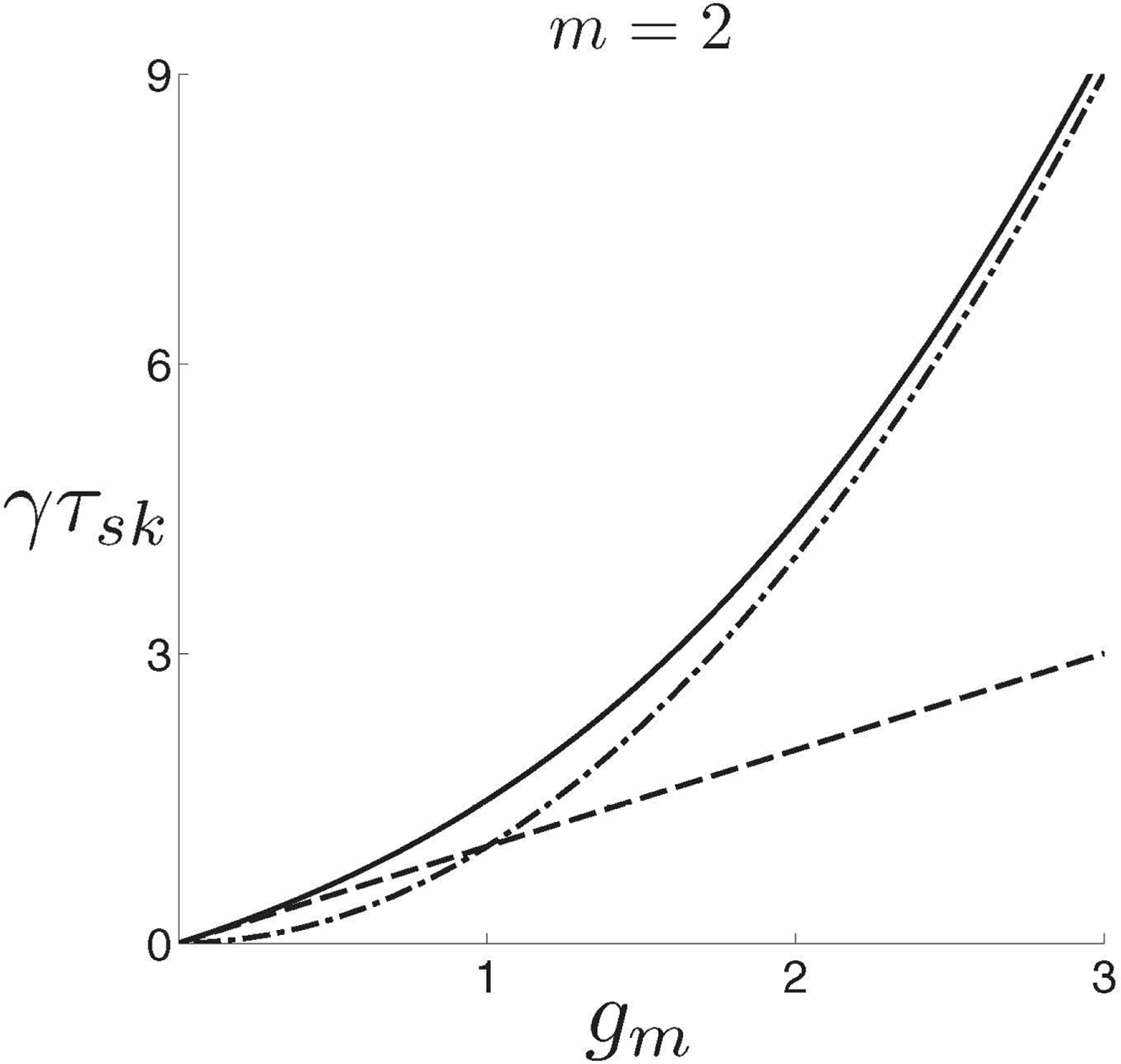
 $$\begin{eqnarray}{\it\gamma}{\it\tau}_{sk}=({\it\gamma}^{sh}{\it\tau}_{sk})^{2},\end{eqnarray}$$
where
 ${\it\gamma}$
is the true growth rate at
 $s\ll d_{w}$
,
 ${\it\gamma}^{sh}$
is the thin-wall estimate (though far behind the applicability region of the thin-wall approximation), and
 $$\begin{eqnarray}{\it\tau}_{sk}\equiv {\it\sigma}d_{w}^{2}={\it\tau}_{w}d_{w}/r_{w}.\end{eqnarray}$$
Finally, we have two distinctly different dispersion relations for the modes interacting with a resistive wall. One is obtained in the standard thin-wall model, which assumes
 $\boldsymbol{b}\boldsymbol{\cdot }\boldsymbol{n}_{w}$
identical on the both sides of the wall:
 $$\begin{eqnarray}{\it\gamma}^{sh}{\it\tau}_{sk}=g_{m}.\end{eqnarray}$$
Another is obtained assuming the same wall to be magnetically thick so that
 $\boldsymbol{b}\boldsymbol{\cdot }\boldsymbol{n}_{w}=0$
behind the wall:
 $$\begin{eqnarray}{\it\gamma}{\it\tau}_{sk}=g_{m}^{2}.\end{eqnarray}$$
In these relations,
 $$\begin{eqnarray}g_{m}\equiv \frac{d_{w}}{r_{w}}\frac{F-W_{w+}}{D_{0}^{sh}},\end{eqnarray}$$
where
 $W_{w+}$
can be disregarded when applied to the fast modes. Then
 $g_{m}$
is determined by two surface integrals over the inner side of the wall. By definition,
 $D_{0}^{sh}$
is a real quantity. The imaginary part of
 $g_{m}$
can appear from
 $F$
only. Note that (8.8) and (8.9), one valid for slow modes with
 $s\gg d_{w}$
and the other for fast modes with
 $s\ll d_{w}$
, have been obtained without restrictions on the plasma models. These relations are derived from (3.13) and (4.1) describing the energy balance outside the plasma, which is a perfect foundation free from uncertainties related to incomplete knowledge of the plasma equilibrium parameters and the perturbation dynamics.
To be precise, (3.14) and (4.1), with complex
 $F$
, should be called energy–torque relations. The toroidal electromagnetic torque exerted on the plasma is
 $$\begin{eqnarray}T\equiv \int _{V_{pl}}R\boldsymbol{e}_{{\it\zeta}}\boldsymbol{\cdot }(\boldsymbol{j}\times \boldsymbol{B})\,\text{d}V=\int _{S_{as}}RB_{{\it\zeta}}\boldsymbol{B}\boldsymbol{\cdot }\text{d}\boldsymbol{S},\end{eqnarray}$$
where
 $S_{as}$
is any axisymmetric surface in the vacuum gap [Reference Pustovitov91, Reference Pustovitov92]. For a magnetic perturbation with a single toroidal harmonic, we obtain in terms of the complex functions used in (4.5):
 $$\begin{eqnarray}T=\frac{\text{i}n}{4}\oint _{wall-}({\it\varphi}_{-}\boldsymbol{b}_{-}^{\ast }-{\it\varphi}_{-}^{\ast }\boldsymbol{b}_{-})\boldsymbol{\cdot }\text{d}\boldsymbol{S}_{w}=n\,\text{Im}\,F,\end{eqnarray}$$
Similarly, for
 $n\neq 0$
and axisymmetric
 $S_{w}$
,
 $\text{Re}({\it\gamma}^{\ast }F)$
will be the Poynting vector flux through the wall.
9. Cylindrical estimates
Equation (8.1) and its reduced versions, (8.8) and (8.9), are valid for toroidal systems without limitations on the plasma shape. For a cylindrical configuration shown in figure 3, each term in (8.1) can be expressed in a form allowing easy estimates and comparisons.
In this geometry, with perturbations prescribed in the form (2.3) the surface integrals turn into
 $$\begin{eqnarray}\oint _{wall}XY^{\ast }\,\text{d}S_{w}=X_{m}Y_{m}^{\ast }S_{w},\end{eqnarray}$$
where
 $S_{w}$
is the full area of the wall surface. When
 $X$
and
 $Y$
are represented by several harmonics, the right-hand side will be a sum over
 $m$
. This can be applied to (4.4) and (4.5).
Another simplification comes from the use of the explicit cylindrical solutions to (7.7) in the wall and to the Laplace equation
 ${\rm\nabla}^{2}{\it\varphi}=0$
for the magnetic potential
 ${\it\varphi}$
in vacuum. For example, in the plasma–wall vacuum gap and behind the wall, such solution for the
 $(m,n)$
harmonic is
 $$\begin{eqnarray}{\it\varphi}_{m}=\frac{R_{0}}{n}\left\{B_{m}^{\text{i}n}\frac{\text{K}_{m}(u)}{\text{K}_{m}^{\prime }(u_{w})}+B_{m}^{out}\frac{\text{I}_{m}(u)}{\text{I}_{m}^{\prime }(u_{w})}\right\}.\end{eqnarray}$$
Here
 $\text{I}_{m}$
and
 $\text{K}_{m}$
are the modified Bessel functions, the prime denotes the derivative with respect to
 $u=nr/R_{0}$
, with
 $2{\rm\pi}R_{0}$
being the length of the system and
 $u_{w}=nr_{w}/R_{0}$
. The complex constants
 $B_{m}^{in}$
and
 $B_{m}^{out}$
must be different at the opposite sides of the wall.
The radial component of
 $\boldsymbol{b}=\boldsymbol{{\rm\nabla}}{\it\varphi}$
is then given by
 $$\begin{eqnarray}b_{r}=b_{m}(r,t)\exp \text{i}(m{\it\theta}-n{\it\zeta})\end{eqnarray}$$
with
 $$\begin{eqnarray}b_{m}=b_{m}^{\text{i}n}+b_{m}^{out},\end{eqnarray}$$
where the first term is the part of
 $b_{m}$
due to the currents in the inner area with respect to the point
 $r$
, and the second one describes the contribution from the outer sources. These functions correspond to the two terms in (9.2). For perturbations with small
 $m$
and
 $n$
, one can use the approximate expressions (valid for
 $nr\ll mR_{0}$
)
 $$\begin{eqnarray}\displaystyle & \displaystyle b_{m}^{\text{i}n}=B_{m}^{\text{i}n}x^{-m-1}, & \displaystyle\end{eqnarray}$$
 $$\begin{eqnarray}\displaystyle & \displaystyle b_{m}^{out}=B_{m}^{out}x^{m-1}, & \displaystyle\end{eqnarray}$$
where
 $x=r/r_{w}$
, while
 $B_{m}^{\text{i}n}$
and
 $B_{m}^{out}$
introduced in (9.2) are the amplitudes of
 $b_{m}^{\text{i}n}$
and
 $b_{m}^{out}$
at
 $x=1$
. Then (9.2) reduces to
 $$\begin{eqnarray}{\it\varphi}_{m}=\frac{r}{m}(b_{m}^{out}-b_{m}^{\text{i}n})=\frac{r}{m}(2b_{m}^{out}-b_{m}).\end{eqnarray}$$
With this approximate relation for a single mode
 $(m,n)$
, we obtain from (4.4) and (4.5)
 $$\begin{eqnarray}W_{w+}=\frac{r_{w}}{2m}{\it\beta}_{m}{\it\beta}_{m}^{\ast }S_{w}\end{eqnarray}$$
and
 $$\begin{eqnarray}F=\frac{r_{w}}{2m}(B_{m}-2B_{m}^{out})B_{m}^{\ast }S_{w},\end{eqnarray}$$
where
 ${\it\beta}_{m}$
and
 $B_{m}$
are, respectively, the amplitudes of
 $b_{m}$
at the outer and inner sides of the wall. Accordingly, for the considered simple case without sources of
 $\boldsymbol{b}$
behind the wall,
 $B_{m}^{out}$
in (9.9) means the field produced by the wall currents. The wall is treated as geometrically thin (
 $d_{w}\ll r_{w}$
), that is why the both equalities contain
 $r_{w}$
. For the magnetically thin wall we could put
 ${\it\beta}_{m}$
and
 $B_{m}$
equal. In the general case, they are different. This is the reason why, finally, (8.9) differs from (8.8).
For the quantity
 $W_{w}$
in (8.1) we can use the approximate relation
 $W_{w}=0$
in the thin-wall limit (
 $s\gg d_{w}$
) and (7.10) in the thick-wall limit
 $(s\ll d_{w})$
.
To express
 $D_{0}^{sh}$
similar to (9.8) and (9.9), we have to solve (4.12) for
 $\boldsymbol{E}$
. If the wall is geometrically thin,
 $E_{r}$
must be small and
 $\boldsymbol{{\rm\nabla}}\boldsymbol{\cdot }\boldsymbol{E}=0$
is approximated by
 $$\begin{eqnarray}mR_{0}E_{{\it\theta}}=nrE_{z}\end{eqnarray}$$
for the
 $(m,n)$
harmonic described by (9.3). Then
 $\boldsymbol{{\rm\nabla}}r\times \boldsymbol{E}\approx -E_{z}\boldsymbol{e}_{{\it\theta}}$
, where the term of the order of
 $nr/(mR_{0})$
is disregarded, and (4.12) yields
 $$\begin{eqnarray}E_{z}=\text{i}{\it\gamma}\frac{r}{m}b_{r}.\end{eqnarray}$$
For perturbations with
 $nr\ll mR_{0}$
we can retain
 $E_{z}$
only in (4.9). It gives then with (9.1) and
 ${\it\sigma}={\it\sigma}_{0}$
:
 $$\begin{eqnarray}D_{0}^{sh}=\frac{r_{w}}{2m^{2}}B_{m}B_{m}^{\ast }S_{w}.\end{eqnarray}$$
With these relations, (8.10) becomes
 $$\begin{eqnarray}g_{m}=\frac{md_{w}}{r_{w}}\left[\left(1-\frac{{\it\beta}_{m}{\it\beta}_{m}^{\ast }}{B_{m}B_{m}^{\ast }}\right)-2\frac{B_{m}^{out}}{B_{m}}\right],\end{eqnarray}$$
where the term in the round brackets must be zero in the thin-wall case
 $({\it\beta}_{m}=B_{m})$
. In the thick-wall limit (
 $|{\it\beta}_{m}|\ll |B_{m}|$
), it can be disregarded as a small correction.
The latter can be easily explained. It follows from (8.2) in combination with (8.8) and (8.9) that
 $$\begin{eqnarray}\frac{d_{w}}{s}=\text{Re}\left\{\begin{array}{@{}ll@{}}\sqrt{g_{m}} & \text{at }d_{w}\ll s\\ g_{m}, & \text{at }d_{w}\gg s.\end{array}\right.\end{eqnarray}$$
This shows that
 $|g_{m}|$
must be large in the thick-wall limit. To make consistent (9.13) and (9.14) at
 $d_{w}\gg s$
, we need
 $2|B_{m}^{out}/B_{m}|\gg r_{w}/(md_{w})$
. Then, with typical
 $r_{w}\gg d_{w}$
and moderate
 $m$
, this will be the dominant contribution in (9.13).
The above means that in both cases, in the thin- (
 $s\gg d_{w}$
) and thick-wall (
 $s\ll d_{w}$
) limits, we can use the relation
 $$\begin{eqnarray}g_{m}=\frac{d_{w}}{r_{w}}{\it\Gamma}_{m},\end{eqnarray}$$
where
 $$\begin{eqnarray}{\it\Gamma}_{m}\equiv -2m\frac{B_{m}^{out}}{B_{m}}=-\frac{2m}{1-x^{2m}+x^{2m}b_{m}/b_{m}^{out}}.\end{eqnarray}$$
The latter equality is obtained with the use of (9.4)–(9.6). It gives
 ${\it\Gamma}_{m}$
as a function of
 $b_{m}/b_{m}^{out}$
at any point in the plasma–wall vacuum gap. In experiments,
 $b_{m}$
can be measured by the magnetic probes. Extracting
 $b_{m}^{out}$
from
 $b_{m}$
requires some additional measurements and processing of data [Reference Pustovitov93, Reference Pustovitov94], but finally
 ${\it\Gamma}_{m}$
can be found without precise knowledge of the plasma parameters. This gives
 $g_{m}$
, and we can use (8.8) and (8.9) either for evaluation of
 ${\it\gamma}_{R}$
and
 ${\it\omega}$
or for comparison of the measured
 ${\it\gamma}_{R}$
and
 ${\it\omega}$
with the model predictions.
Moving into the range of smaller
 $s/d_{w}\ll 1$
, we will eventually approach the ideal-wall limit at
 $s=0$
. In classical stability theory [Reference Bernstein, Frieman, Kruskal and Kulsrud3–Reference Goedbloed and Poedts8], it is introduced by
 $\boldsymbol{n}_{w}\times \boldsymbol{E}=\boldsymbol{n}_{w}\boldsymbol{\cdot }\boldsymbol{b}=0$
at the wall. In the cylindrical model, this reduces to
 $B_{m}=0$
. Then the presented expressions in terms of
 $B_{m}$
give us infinite
 $g_{m}$
and
 ${\it\gamma}{\it\tau}_{sk}$
. The latter contains
 ${\it\tau}_{sk}$
which is also infinite for an ideal wall. Therefore, finding the ideal-wall
 ${\it\gamma}$
requires more careful actions than a simple substitution of
 $s=0$
into the otherwise reliable and informative formulas for the fast RWMs. The transition to ideal MHD modes for large
 $g_{m}$
and
 ${\it\gamma}{\it\tau}_{sk}$
is discussed in § 17.
10. Relation to other RWM models
We introduced
 ${\it\Gamma}_{m}$
in (9.15) to make easier comparisons between the existing models. This is exactly the same as
 ${\it\Gamma}_{m}$
in the equation
 $$\begin{eqnarray}{\it\tau}_{w}\frac{\partial B_{m}}{\partial t}={\it\Gamma}_{m}B_{m}-{\it\Gamma}_{m}^{0}B_{m}^{ext},\end{eqnarray}$$
which has been used in the thin-wall analysis of RWMs and related effects in [Reference Pustovitov77, Reference Pustovitov84, Reference Pustovitov and Villone85, Reference Pustovitov and Mayorova90, Reference Pustovitov93, Reference Pustovitov95]. Here
 ${\it\Gamma}_{m}^{0}=-2m$
for
 $m\neq 0$
or
 ${\it\Gamma}_{m}^{0}=-2$
for
 $m=0$
and
 $B_{m}^{ext}$
is the contribution to
 $B_{m}$
due to sources behind the wall. For example,
 $B_{m}^{ext}$
may be the error field and/or the field of the correction or feedback coils. Equation (10.1) is an integral cylindrical consequence of (7.7). At constant or zero
 $B_{m}^{ext}$
it gives the dispersion relation
 $$\begin{eqnarray}{\it\gamma}{\it\tau}_{w}={\it\Gamma}_{m},\end{eqnarray}$$
which is equivalent to (8.8) combined with (8.7) and (9.15) or to (3.10) in [Reference Okabayashi, Bialek, Bondeson, Chance, Chu, Garofalo, Hatcher, In, Jackson and Jayakumar17].
Equations similar to (10.1) can be found in [Reference Hender, Wesley, Bialek, Bondeson, Boozer, Buttery, Garofalo, Goodman, Granetz and Gribov2, Reference Chu and Okabayashi10, Reference Garofalo, Jensen and Strait13, Reference Chu, Bondeson, Chance, Liu, Garofalo, Glasser, La Haye, Lao and Navratil14, Reference Chu, Chan, Chance, Edgell, Garofalo, Glasser, Guo, Humphreys, Jensen and Kim38, Reference Frassinetti, Brunsell and Drake39, Reference Chu, Chance, Glasser and Okabayashi43, Reference Chance, Chu, Okabayashi and Turnbull73]. The lumped-parameter model [Reference Strait, Bialek, Bogatu, Chance, Chu, Edgell, Garofalo, Jackson, Jensen and Johnson12, Reference Okabayashi, Bialek, Bondeson, Chance, Chu, Garofalo, Hatcher, In, Jackson and Jayakumar17] operates with a system of several equations which also reduces to (10.1).
Equation (9.16) gives a simple connection to any RWM model, including those that prescribe the plasma dynamics and present
 ${\it\Gamma}_{m}$
as a function of plasma parameters. Only
 $b_{m}/b_{m}^{out}$
is needed to find
 ${\it\Gamma}_{m}$
and make a step towards (8.8) and (8.9). Such a procedure has been employed in [Reference Pustovitov96], where the Boozer model [Reference Boozer97, Reference Boozer98] was analysed to find its hidden implications and make possible their comparison with experimental results.
Instead of
 $b_{m}/b_{m}^{out}$
, one can use the ratio
 $rb_{m}^{\prime }/b_{m}$
. This follows from [Reference Pustovitov77, Reference Pustovitov and Mayorova90, Reference Pustovitov96]
 $$\begin{eqnarray}\frac{rb_{m}^{\prime }}{b_{m}}=-(m+1)-\frac{2m{\it\Gamma}_{m}x^{2m}}{2m+{\it\Gamma}_{m}(1-x^{2m})}\end{eqnarray}$$
for the plasma–wall vacuum gap, which comes from (9.4) and (9.16) with approximate (9.5) and (9.6) that give
 $$\begin{eqnarray}2mb_{m}^{out}=rb_{m}^{\prime }+(m+1)b_{m}.\end{eqnarray}$$
Here the prime means the radial derivative, and
 $x=r/r_{w}$
.
In the Fitzpatrick–Aydemir model [Reference Fitzpatrick and Aydemir99], the thin-wall dispersion relations are expressed through
 $rb_{m}^{\prime }/b_{m}$
at the plasma surface
 $S_{pl}$
. With (10.3) they can be cast in the form of (10.2), which facilitated the detailed analysis of their consequences and comparison to the Boozer model in [Reference Pustovitov100]. The boundary conditions in terms of
 $rb_{m}^{\prime }/b_{m}$
at the plasma edge were also prescribed in the models in [Reference Bondeson and Ward32, Reference Betti and Freidberg36].
Equations (9.16) and (10.3) show that the plasma properties enter the task through either
 $b_{m}/b_{m}^{out}$
or
 $rb_{m}^{\prime }/b_{m}$
at
 $S_{pl}$
. These quantities may be complex making thereby
 $$\begin{eqnarray}{\it\Gamma}_{m}={\it\tau}_{w}({\it\gamma}_{0}+in{\it\Omega}_{0}),\end{eqnarray}$$
where, according to (10.1), real
 ${\it\gamma}_{0}$
and
 ${\it\Omega}_{0}$
are the natural instantaneous decay/growth rate of the mode and the angular frequency of its toroidal rotation (in the thin-wall approximation under fixed
 $B_{m}^{ext}$
or
 $B_{m}^{ext}=0$
). In the ideal MHD,
 ${\it\gamma}^{2}$
must be real, in which case only one of these parameters survives in (10.5). This may hold true even if the resistive wall is present, though only in the thin-wall approximation [Reference Chu and Okabayashi10, Reference Haney and Freidberg35, Reference Chu, Chance, Glasser and Okabayashi43, Reference Medvedev and Pustovitov44, Reference Chu and Ichiguchi46]. Then the plasma interaction with the resistive wall is described by a single number.
Such simplification is not an attribute of some cylindrical models only. In the thin-wall code VALEN, the perturbation produced by the plasma is also modelled as a single mode described by a real
 ${\it\Gamma}_{m}$
[Reference Bialek, Boozer, Mauel and Navratil41, Reference Mauel, Bialek, Boozer, Cates, James, Katsuro-Hopkins, Klein, Liu, Maurer and Maslovsky45, Reference Katsuro-Hopkins, Sabbagh, Bialek, Park, Bak, Chung, Hahn, Kim, Kwon and Lee82].
The approach starting from (4.1), with a detailed description of the outer region and leading to (8.1), (8.8) and (8.9) allows a unified treatment with different plasma models (ideal or non-ideal) as replaceable parts in the full task. Equations (9.16) and (10.3) also show a straightforward path for extension of the previous studies from slow to fast RWMs since both (8.8) and (8.9) contain the same
 $g_{m}$
or, finally,
 ${\it\Gamma}_{m}$
.
11. Plasma response
To make definite conclusions from the derived dispersion relations (8.8) and (8.9), we have to know the properties of
 $g_{m}$
. This quantity was defined by (8.10) through the integrals quadratic in
 $\boldsymbol{b}$
and
 $\boldsymbol{E}$
. Equations (9.15) and (9.16) show that, in the cylindrical limit,
 $g_{m}$
is proportional to the ratio
 $B_{m}^{out}/B_{m}$
, where
 $$\begin{eqnarray}B_{m}=B_{m}^{out}+B_{m}^{pl}\end{eqnarray}$$
and
 $B_{m}^{pl}$
is the contribution to
 $B_{m}$
from the plasma. Therefore,
 $g_{m}$
is determined by the plasma response to the perturbation from outside,
 $B_{m}^{out}$
.
The fusion plasma too easily responds to perturbations that cannot be eliminated in advance, or properly counteracted. At the same time, to reach the goals of ITER, JT-60SA and similar projects, we need high accuracy in the predictions of these responses.
The general problem of the plasma response was recently discussed in [Reference Liu, Kirk and Nardon101–Reference Reiman, Ferraro, Turnbull, Park, Cerfon, Evans, Lanctot, Lazarus, Liu and McFadden104]. In [Reference Liu, Kirk and Nardon101], the linear plasma response to resonant magnetic perturbation (RMP) and non-resonant perturbation fields was computed using the MHD code MARS-F. The response of resonant harmonics was found to be sensitive to the plasma resistivity and the toroidal rotation, while that of non-resonant harmonics was mostly sensitive to the equilibrium plasma pressure. This was a systematic study with various plasma parameters and coil configurations which led the authors to the conclusion that it is still questionable to apply these results directly to the edge localized modes (ELMs) mitigation experiments due to limitations of the model. In [Reference Wade, Nazikian, Battaglia, Buttery, Degrassie, Evans, Fenstermacher, Ferraro, Grierson and Hansen103], the evidence from DIII-D experiments was presented indicating that several effects are important in the overall plasma response, so that even the vacuum model, the simplest description of the tokamak plasma response to 3-D fields, is predicted to be quite complex. In [Reference Turnbull102], an overall conclusion was that none of the analysed linear and nonlinear models are fully satisfactory. In [Reference Reiman, Ferraro, Turnbull, Park, Cerfon, Evans, Lanctot, Lazarus, Liu and McFadden104], a significant disagreement has been seen between solutions of the VMEC stellarator equilibrium code and solutions of tokamak perturbative 3-D equilibrium codes.
A positive allusion in this and similar critical statements is that diagnostic capabilities and resolution have reached a level of high art. However, even with the best local measurements in the plasma, one cannot expect from theory a comprehensive picture for a very simple reason: there are too many unknowns in the problem. To solve the Maxwell equations, one needs complete knowledge of the current density distribution
 $\boldsymbol{j}(\boldsymbol{r})$
and the boundary conditions. The fact that the magnetic field
 $\boldsymbol{B}(\boldsymbol{r})$
is the integral function of all currents in the plasma means that the local plasma response will always be calculated with some error. On the other hand, the same integral nature of
 $\boldsymbol{B}(\boldsymbol{r})$
makes these predictions quite reliable ‘in an average sense’. That is why even the cylindrical model gives useful insight into the physics of kink-like instabilities.
In the model discussed in the two previous sections,
 $$\begin{eqnarray}B_{m}^{out}=B_{m}^{w}+B_{m}^{er}+B_{m}^{f},\end{eqnarray}$$
which includes several inputs: from the wall,
 $B_{m}^{w}$
, from some unaccounted sources (error field),
 $B_{m}^{er}$
and from the correction coils,
 $B_{m}^{f}$
. The latter can be used as a known perturbation to find
 ${\it\Gamma}_{m}$
or
 $g_{m}$
by the measured plasma reaction
 $B_{m}^{pl}$
, as described in [Reference Chu and Okabayashi10, Reference Garofalo, Jensen, Johnson, La Haye, Navratil, Okabayashi, Scoville, Strait, Baker and Bialek11, Reference Reimerdes, Hender, Sabbagh, Bialek, Chu, Garofalo, Gryaznevich, Howell, Jackson and La Haye21, Reference Sontag, Sabbagh, Zhu, Menard, Bell, Bialek, Bell, Gates, Glasser and Leblanc29, Reference Reimerdes, Bialek, Chance, Chu, Garofalo, Gohil, In, Jackson, Jayakumar and Jensen75, Reference Pustovitov77, Reference Pustovitov93]. To avoid confusion, we note that the dispersion relations given by (8.1), (8.8) and (8.9) are obtained for the ‘open loop’ system, which means
 $B_{m}^{er}+B_{m}^{f}=\text{const.}$
or zero. The feedback control is incorporated into the model though
 $B_{m}^{ext}$
in (10.1), as described, for example, in [Reference Hender, Wesley, Bialek, Bondeson, Boozer, Buttery, Garofalo, Goodman, Granetz and Gribov2, Reference Chu and Okabayashi10, Reference Frassinetti, Brunsell and Drake39, Reference Bialek, Boozer, Mauel and Navratil41–Reference Mauel, Bialek, Boozer, Cates, James, Katsuro-Hopkins, Klein, Liu, Maurer and Maslovsky45, Reference Gribov and Pustovitov72, Reference Bondeson, Liu, Gregoratto, Gribov and Pustovitov76, Reference Pustovitov and Mayorova90, Reference Pustovitov95].
If
 ${\it\Gamma}_{m}$
is found in some particular case, the main questions are whether it will remain the same at varying amplitude of
 $\boldsymbol{b}^{out}$
and fixed plasma parameters and if it will depend on
 ${\it\gamma}$
or not?
The first question can be reformulated to whether the plasma reacts to
 $\boldsymbol{b}^{out}$
as a linear system? In view of the practical applications, this can be also discussed in terms of the mode rigidity [Reference Chu and Okabayashi10, Reference Okabayashi, Bialek, Bondeson, Chance, Chu, Garofalo, Hatcher, In, Jackson and Jayakumar17, Reference Okabayashi, Bogatu, Chance, Chu, Garofalo, In, Jackson, La Haye, Lanctot and Manickam24, Reference Igochine and Igochine40, Reference Medvedev and Pustovitov44, Reference Chance, Chu, Okabayashi and Turnbull73, Reference Pustovitov and Mayorova90, Reference Pustovitov93, Reference Okabayashi, Bialek, Chance, Chu, Fredrickson, Garofalo, Gryaznevich, Hatcher, Jensen and Johnson105, Reference Baruzzo, Bolzonella, Liu, Manduchi, Marchiori, Soppelsa, Takechi and Villone106] which means the invariance of the mode structure in the plasma at fixed parameters of the equilibrium configuration during magnetic feedback stabilization and/or error field correction [Reference Okabayashi, Bialek, Chance, Chu, Fredrickson, Garofalo, Gryaznevich, Hatcher, Jensen and Johnson105].
The linearity is one of the foundation principles of most stability theories. Its validity or relevance can be proved by experiment only. In the DIII-D tokamak, the linearity of the plasma response was found to be a good assumption for the externally applied resonant magnetic fields
 $10^{-4}{-}10^{-3}$
of the main toroidal field [Reference Reimerdes, Bialek, Chance, Chu, Garofalo, Gohil, In, Jackson, Jayakumar and Jensen75]. A linear plasma response to the applied error field was confirmed in both the JET and the Mega Ampère Spherical Tokamak (MAST) [Reference Chapman, Hender, Howell, Erents, Gryaznevich, Shibaev, Stamp, De La Luna, Savchkov and Scannell107].
It is clear that such linearity cannot be expected just near the stability boundary. In [Reference Lanctot, Reimerdes, Garofalo, Chu, Liu, Strait, Jackson, La Haye, Okabayashi and Osborne47, Reference Lanctot, Reimerdes, Garofalo, Chu, Hanson, Liu, Navratil, Bogatu, In and Jackson48], the predictions of linear ideal MHD were compared with measurements of the external plasma response to applied
 $n=1$
magnetic perturbations in rotating, H-mode discharges on the DIII-D tokamak. The plasma response calculated with the MARS-F code was found adequate to describe the plasma response for values of
 ${\it\beta}_{N}$
up to approximately 75 % [Reference Lanctot, Reimerdes, Garofalo, Chu, Liu, Strait, Jackson, La Haye, Okabayashi and Osborne47] or 80 % [Reference Lanctot, Reimerdes, Garofalo, Chu, Hanson, Liu, Navratil, Bogatu, In and Jackson48] of the no-wall stability limit
 ${\it\beta}_{N}^{\mathit{no\,wall}}$
. It is interesting that, for higher plasma pressures, the ideal MHD model overestimated the perturbed field (by a factor of 1.5–3 [Reference Lanctot, Reimerdes, Garofalo, Chu, Liu, Strait, Jackson, La Haye, Okabayashi and Osborne47]). This is actually good news because it means that, in this particular case, the plasma behaves better near the stability limit than is predicted by the ideal linear theory. At least, this does not compromise the linearity but rather indicates the increasing importance of stabilizing non-ideal effects [Reference Lanctot, Reimerdes, Garofalo, Chu, Liu, Strait, Jackson, La Haye, Okabayashi and Osborne47].
With linear plasma response, the ratio
 $B_{m}^{out}/B_{m}$
and, accordingly,
 $g_{m}$
and
 ${\it\Gamma}_{m}$
defined by (9.15) and (9.16) must be independent of
 $B_{m}$
. In the following analysis of (8.8) and (8.9), we also assume that
 $g_{m}$
does not depend on
 ${\it\gamma}$
. Then (8.8) and (8.9) will give us the resolved dispersion relations with the right-hand sides depending on the plasma parameters only.
The latter assumption is naturally justified in the ideal MHD models for RWMs, where the plasma inertia is disregarded [Reference Chu and Okabayashi10, Reference Chu, Bondeson, Chance, Liu, Garofalo, Glasser, La Haye, Lao and Navratil14, Reference Turnbull, Brennan, Chu, Lao and Snyder19, Reference Haney and Freidberg35, Reference Chu, Chan, Chance, Edgell, Garofalo, Glasser, Guo, Humphreys, Jensen and Kim38, Reference Chu, Chance, Glasser and Okabayashi43, Reference Medvedev and Pustovitov44, Reference Chu and Ichiguchi46, Reference Shiraishi, Aiba, Miyato and Yagi49, Reference Strumberger, Merkel, Sempf and Günter68–Reference Portone, Villone, Liu, Albanese and Rubinacci70, Reference Chance, Chu, Okabayashi and Turnbull73, Reference Liu, Chu, Guo, Villone, Albanese, Ambrosino, Baruzzo, Bolzonella, Chapman and Garofalo108] because RWMs are considered as slow modes. Indeed, if
 ${\it\delta}K=0$
in (3.14) and the plasma is assumed ideal (
 $N=0$
), the flux
 $F$
does not bring a dependence on
 ${\it\gamma}$
in (8.10). For a non-ideal plasma, this will be true when
 $|N|\ll |F|$
.
12. Separation of the plasma response from the magnetic signals
We have already mentioned that the plasma response can be measured. This was with references to the schemes based on the single-mode approach. The method, however, has a perfect theoretical background. Properly integrating the Maxwell equations over the volume
 $V$
bounded by the toroidal surface
 $S$
in the plasma–wall vacuum gap one obtains
 $$\begin{eqnarray}\frac{1}{4{\rm\pi}}\oint _{s}\left[(\boldsymbol{n}\times \boldsymbol{B})\times \frac{\boldsymbol{r}-\boldsymbol{r}_{s}}{|\boldsymbol{r}-\boldsymbol{r}_{s}|^{3}}+(\boldsymbol{n}\boldsymbol{\cdot }\boldsymbol{B})\frac{\boldsymbol{r}-\boldsymbol{r}_{s}}{|\boldsymbol{r}-\boldsymbol{r}_{s}|^{3}}\right]\text{d}S=\left\{\begin{array}{@{}ll@{}}-\boldsymbol{B}^{out}(\boldsymbol{r}) & \text{if }\boldsymbol{r}\in V\\ \boldsymbol{B}^{pl}(\boldsymbol{r}) & \text{if }\boldsymbol{r}\notin V\cup S,\end{array}\right.\end{eqnarray}$$
where
 $\boldsymbol{r}$
is the observation point,
 $\boldsymbol{r}_{s}$
is the point at the surface
 $S$
and
 $\boldsymbol{n}$
is the outward unit normal to
 $S$
. This is a precise equality allowing the separation of the plasma-produced magnetic field
 $\boldsymbol{B}^{pl}$
from the total magnetic field
 $\boldsymbol{B}=\boldsymbol{B}^{pl}+\boldsymbol{B}^{out}$
[Reference Pustovitov94]. If
 $\boldsymbol{n}\boldsymbol{\cdot }\boldsymbol{B}=0$
, which happens when
 $S$
coincides with a magnetic surface (for example, the plasma boundary), (12.1) gives the ‘virtual casing principle’ solution [Reference Shafranov and Zakharov109, Reference Hirshman, Lazarus, Hanson, Knowlton and Lao110]. Applications based on (12.1) or its equivalents are well known in the tasks of stellarator equilibrium [Reference Merkel111].
With
 $\boldsymbol{B}$
expressed by (3.3), this can be divided on two equations, for
 $\boldsymbol{B}_{0}$
and
 $\boldsymbol{b}$
. If the perturbation
 $\boldsymbol{b}$
could be measured or prescribed at the surface, then calculating the left-hand side of (12.1) we obtain both
 $\boldsymbol{b}^{pl}$
and
 $\boldsymbol{b}^{out}$
.
Such application of the mathematically strict result will suffer from the incomplete information provided by the magnetic measurements at the integration surface
 $S$
. The accuracy of the method based on the measured
 $\boldsymbol{b}$
can be improved by comparing
 $\boldsymbol{b}^{out}$
thus found from (12.1) against
 $\boldsymbol{b}^{out}$
precisely calculated by the Biot–Savart law with known currents in the external conductors.
In a full-scale experiment, only the field
 $\boldsymbol{b}^{\,f}$
from the correction or feedback coils may be known, which is a part of
 $$\begin{eqnarray}\boldsymbol{b}^{out}=\boldsymbol{b}^{w}+\boldsymbol{b}^{er}+\boldsymbol{b}^{\,f},\end{eqnarray}$$
where
 $\boldsymbol{b}^{w}$
is the contribution due to the currents in the wall, and
 $\boldsymbol{b}^{er}$
describes the error field (usually unknown, but, presumably, static). In the single-mode case, when (12.2) reduces to (11.2),
 $\boldsymbol{b}^{w}$
and
 $\boldsymbol{b}^{\,f}$
have similar structure, which cannot be expected in a real experiment. Their difference and the dynamically evolving
 $\boldsymbol{b}^{w}$
itself can be evaluated by finding
 $\boldsymbol{b}^{out}-\boldsymbol{b}^{\,f}$
after integration in (12.1). Such extraction of
 $\boldsymbol{b}^{w}$
from the measured
 $\boldsymbol{b}$
can be used in experiments with a control of plasma stability against RWMs or ELMs, with probing the plasma with externally applied RMPs [Reference Chu and Okabayashi10, Reference Garofalo, Jensen, Johnson, La Haye, Navratil, Okabayashi, Scoville, Strait, Baker and Bialek11, Reference Reimerdes, Hender, Sabbagh, Bialek, Chu, Garofalo, Gryaznevich, Howell, Jackson and La Haye21, Reference Sontag, Sabbagh, Zhu, Menard, Bell, Bialek, Bell, Gates, Glasser and Leblanc29, Reference Lanctot, Reimerdes, Garofalo, Chu, Liu, Strait, Jackson, La Haye, Okabayashi and Osborne47, Reference Lanctot, Reimerdes, Garofalo, Chu, Hanson, Liu, Navratil, Bogatu, In and Jackson48, Reference Reimerdes, Bialek, Chance, Chu, Garofalo, Gohil, In, Jackson, Jayakumar and Jensen75, Reference Pustovitov77, Reference Pustovitov93, Reference Gryaznevich, Liu, Hender, Howell, Beurskens, Chapman, Challis, Joffrin, Koslowski, Buratti and Solano112] or in the test blanket module error field simulation experiments [Reference Schaffer, Snipes, Gohil, De Vries, Evans, Fenstermacher, Gao, Garofalo, Gates and Greenfield113]. As a part of separation of different inputs to
 $\boldsymbol{b}$
, knowledge of
 $\boldsymbol{b}^{w}$
could be useful for optimizing the spectrum of
 $\boldsymbol{b}^{\,f}$
and for improving the wall model.
Equation (12.1) is free from any assumption on the plasma because it is derived from the Maxwell equations only. Therefore, the diagnostics based on measurements of
 $\boldsymbol{b}$
combined with (12.1) can be a universal tool in testing various theoretical predictions and suggestions such as the linear plasma response and possible mode rigidity [Reference Chu and Okabayashi10, Reference Okabayashi, Bialek, Bondeson, Chance, Chu, Garofalo, Hatcher, In, Jackson and Jayakumar17, Reference Okabayashi, Bogatu, Chance, Chu, Garofalo, In, Jackson, La Haye, Lanctot and Manickam24, Reference Igochine and Igochine40, Reference Baruzzo, Bolzonella, Liu, Manduchi, Marchiori, Soppelsa, Takechi and Villone106]. Equation (12.1) can also be used to complement the methods of detecting the approach to the stability boundary in tokamaks, stellarators and pinches.
Equations (3.1) and (3.2) describe the plasma dynamics in terms of full
 $\boldsymbol{b}$
. Modelling of the experiments with RMPs or feedback control of plasma stability is always aimed at finding an optimal
 $\boldsymbol{b}^{\,f}$
. This means
 $\boldsymbol{b}^{\,f}$
provoking a desired plasma reaction. With unlimited degrees of freedom, the problem becomes tractable when the main ‘resonances’ are established. In the CarMa code, that proved to be the best in RWM studies, the plasma response matrix is found by calculating the coupling of the linearly perturbed MHD equilibria and 3-D eddy current via the control surface method. This strategy is described in detail [Reference Albanese, Liu, Portone, Rubinacci and Villone69–Reference Villone, Liu, Paccagnella, Bolzonella and Rubinacci71] as a sequence of actions. The separation of
 $\boldsymbol{b}^{pl}$
and
 $\boldsymbol{b}^{out}$
from
 $\boldsymbol{b}=\boldsymbol{b}^{pl}+\boldsymbol{b}^{out}$
performed in the CarMa is actually equivalent to and proved to be correct by (12.1) [Reference Pustovitov94].
13. Comparison of thin- and thick-wall predictions
Two different dispersion relations, (8.8) and (8.9), represent two asymptotes of (8.1). One is valid at
 $d_{w}\ll s$
and the other at
 $d_{w}\gg s$
, which means, respectively, the wall thin or thick compared to the skin depth. It follows from (8.2) that
 $$\begin{eqnarray}\frac{d_{w}}{s}=\text{Re}\sqrt{{\it\gamma}{\it\tau}_{sk}}.\end{eqnarray}$$
Accordingly, the modes with
 $d_{w}\ll s$
can be called slow RWMs, while the modes with
 $d_{w}\gg s$
are fast RWMs. This refers to
 $|{\it\gamma}|$
only irrespective of the origin of the mode. Then ‘RWM’ is a generic name indicating that the mode can dissipate its energy in the resistive wall. This can cover the conventional RWMs, tearing modes, ELM or disruption precursors and other modes that are detected by the magnetic probes in the plasma–wall vacuum gap.
The key quantity determining whether the mode should be qualified and treated as slow of fast RWM is
 $|{\it\gamma}|{\it\tau}_{sk}$
. To be slow, the mode should have small growth (or decay) rate and small rotational frequency. The fast RWM may have either
 $|{\it\gamma}_{R}|$
or
 ${\it\omega}$
large. This means, in particular, that the modes with the same
 ${\it\gamma}_{R}{\it\tau}_{sk}$
but essentially different
 ${\it\omega}{\it\tau}_{sk}$
may belong to the different classes.
In the discussions of the ‘conventional’ RWMs, always
 ${\it\tau}_{w}$
is used as a characteristic time scale [Reference Chu and Okabayashi10–Reference Okabayashi, Matsunaga, Degrassie, Heidbrink, In, Liu, Reimerdes, Solomon, Strait and Takechi25, Reference Sabbagh, Sontag, Bialek, Gates, Glasser, Menard, Zhu, Bell, Bell and Bondeson28–Reference Takechi, Matsunaga, Aiba, Fujita, Ozeki, Koide, Sakamoto, Kurita, Isayama and Kamada30, Reference Haney and Freidberg35–Reference Chu and Ichiguchi46, Reference Chu, Greene, Jensen, Miller, Bondeson, Johnson and Mauel50–Reference Chance, Chu, Okabayashi and Turnbull73], and the RWMs are described as the modes with
 ${\it\gamma}_{R}$
of the order of
 $1/{\it\tau}_{w}$
. Our analysis also includes faster modes. Then
 ${\it\tau}_{sk}$
becomes a more convenient parameter, as illustrated by the dispersion relations in the easily comparable compact forms of (8.8) and (8.9).
These two expressions give the same result at
 $g_{m}=1$
corresponding to
 $s=d_{w}$
. Strictly speaking, this lies in between the applicability regions of these relations (
 $s\gg d_{w}$
and
 $s\ll d_{w}$
, respectively). However, it is numerically proved [Reference Pustovitov and Yanovskiy89, Reference Pustovitov and Yanovskiy114–Reference Villone and Pustovitov116] that (8.8) and (8.9) give quite accurate estimates of
 ${\it\gamma}$
even in the intermediate range of
 $s/d_{w}$
. This is illustrated by figure 5 for the locked modes, where the straight line corresponds to the thin-wall prediction by (8.8), the dashed-dotted parabolic line represents (8.9) and the solid curve shows
 ${\it\gamma}{\it\tau}_{sk}$
numerically found from the dispersion relation
 $$\begin{eqnarray}g_{m}=\sqrt{{\it\gamma}{\it\tau}_{sk}}\frac{\text{K}_{m-1}(y_{i})\text{I}_{m-1}(y_{e})-\text{I}_{m-1}(y_{i})\text{K}_{m-1}(y_{e})}{\text{K}_{m}(y_{i})\text{I}_{m-1}(y_{e})+\text{I}_{m}(y_{i})\text{K}_{m-1}(y_{e})}\end{eqnarray}$$
equivalent to (13) in [Reference Pustovitov and Yanovskiy89] or to (32) in [Reference Pustovitov and Yanovskiy114]. Here,
 $\text{I}$
and
 $\text{K}$
are the modified Bessel functions,
 $y_{i}$
and
 $y_{e}$
are the values of
 $$\begin{eqnarray}y=\sqrt{{\it\gamma}{\it\tau}_{sk}}\frac{r}{d_{w}}\end{eqnarray}$$
at the inner (
 $r=r_{w}$
) and at the outer (
 $r=r_{w}+d_{w}$
) sides of the wall so that
 $y_{e}-y_{i}=\sqrt{{\it\gamma}{\it\tau}_{sk}}$
. It can be shown that (13.2) reduces to (8.8) at
 $s\gg d_{w}$
and to (8.9) at
 $s\ll d_{w}$
.
Calculated dependence of
 ${\it\gamma}$
on
 $g_{m}$
for the locked modes with
 $m=2$
and the wall with
 $d_{w}/r_{w}=0.02$
. The solid line is the cylindrical result given by (13.2), the dashed line shows the thin-wall prediction by (8.8), while the dashed-dotted line corresponds to the thick-wall limit described by (8.9). (Figure 3 from [Reference Pustovitov and Yanovskiy114]. Figure courtesy of Yanovskiy.)

Equation (13.2) is obtained in the cylindrical approximation by using (9.2) for the vacuum region and similar solution to (7.7) for the wall without expansion in radius or in
 $s/d_{w}$
. Much simpler equations (8.8) and (8.9) are thin- and thick-wall asymptotes. Comparison with the results of toroidal calculations [Reference Villone and Pustovitov116] proves that these cylindrical equations are quite reliable.
The upper curve in figure 5 smoothly connects the thin-wall and thick-wall regimes, while (8.8) and (8.9), if used behind their inherent limitations on
 $g_{m}$
, will give us a sharper transition at
 $g_{m}=1$
when
 $s=d_{w}$
. This occurs at
 ${\it\gamma}={\it\gamma}_{l}$
with
 ${\it\gamma}_{l}{\it\tau}_{sk}=1$
or
 $$\begin{eqnarray}{\it\gamma}_{l}{\it\tau}_{w}=r_{w}/d_{w},\end{eqnarray}$$
where
 ${\it\tau}_{w}$
is introduced by (4.8). This simple formula can be used as a convenient definition of the point behind which the thin-wall evaluation of
 ${\it\gamma}$
becomes less reliable than the thick-wall estimates. Both
 $r_{w}/d_{w}$
and
 ${\it\tau}_{w}$
that define
 ${\it\gamma}_{l}$
here are the parameters (at least, approximately) known for each device. Comparing the measured or calculated growth rate
 ${\it\gamma}$
with
 ${\it\gamma}_{l}$
one can easily decide whether or not the skin effect plays a role in the energy balance. Equation (13.4) gives the lower boundary for the fast non-rotating RWMs.
For the purely rotating modes (with
 ${\it\gamma}_{R}=0$
) we have from (13.1)
 $$\begin{eqnarray}\frac{d_{w}}{s}=\sqrt{\frac{n{\it\omega}{\it\tau}_{sk}}{2}}.\end{eqnarray}$$
If
 $d_{w}/s\gg 1$
, this regime must be described by (8.9) implying that
 $$\begin{eqnarray}g_{m}=(1+i)d_{w}/s\end{eqnarray}$$
in this particular case. With this
 $g_{m}$
, the thin-wall dispersion relation (8.8) predicts quite severe instability with
 $\text{Re}{\it\gamma}^{sh}{\it\tau}_{sk}=d_{w}/s$
in obvious contradiction to the initial assumption that
 ${\it\gamma}_{R}=0$
. This dramatic disagreement in the predictions of (8.8) and (8.9) is much more serious than a qualitative difference in
 ${\it\gamma}$
of the order of 30 % at
 $d_{w}=s$
in figure 5 for the modes with
 ${\it\omega}=0$
. It shows that these two approaches may lead to essentially different conclusions on the stability boundaries for the rotating modes.
14. Application of simple RWM models to real devices
Equations (13.4) and (13.5) suggest that the choice between the two possibilities (thin- or thick-wall modelling) depends on
 $r_{w}/d_{w}$
, if the RWM dynamics is described in terms of
 ${\it\gamma}{\it\tau}_{w}$
or
 ${\it\omega}{\it\tau}_{w}$
.
While
 $r_{w}/d_{w}$
naturally appears as a key parameter in our analysis, it is difficult (or even impossible) to find this ratio in papers on plasma stability. The walls are usually non-circular. Also, their thickness is not a constant, the conductivity is not uniform, they have cuts and ports. An example is shown in figure 6 (from the paper [Reference Sakasai, Masaki, Shibama, Sakurai, Hayashi, Nakamura, Ozaki, Yokoyama, Seki and Shibanuma117] on manufacturing and development of JT-60SA vacuum vessel and divertor). Ambiguity in the definitions of
 $r_{w}$
and
 $d_{w}$
and other parameters of interest is an attribute of all models representing a real device in a simplified form. This extends even to the majority of stability codes. For example, the walls are often treated as axisymmetric and poloidally continuous [Reference Shiraishi, Aiba, Miyato and Yagi49, Reference Bondeson, Liu, Gregoratto, Gribov and Pustovitov76, Reference Strumberger, Günter, Merkel, Riondato, Schwarz, Tichmann and Zehrfeld78, Reference Zheng and Kotschenreuther88, Reference Liu, Chu, Guo, Villone, Albanese, Ambrosino, Baruzzo, Bolzonella, Chapman and Garofalo108, Reference Villone and Pustovitov116, Reference Liu, Chapman, Chu, Reimerdes, Villone, Albanese, Ambrosino, Garofalo, Gimblett and Hastie118–Reference Villone, Chiariello, Mastrostefano, Pironti and Ventre121]. Sometimes, the 2-D wall approximation is qualitatively not good enough to describe even the wall response itself (i.e. in the absence of the plasma) [Reference Liu, Chu, Guo, Villone, Albanese, Ambrosino, Baruzzo, Bolzonella, Chapman and Garofalo108]. On the other hand, it is known that a much simpler single-mode cylindrical model can give quite reliable forecasts with good agreement with experimental and numerical results [Reference Hender, Wesley, Bialek, Bondeson, Boozer, Buttery, Garofalo, Goodman, Granetz and Gribov2, Reference Chu and Okabayashi10, Reference Strait, Bialek, Bogatu, Chance, Chu, Edgell, Garofalo, Jackson, Jensen and Johnson12, Reference Strait, Bialek, Bogatu, Chance, Chu, Edgell, Garofalo, Jackson, Jayakumar and Jensen15, Reference Bialek, Boozer, Mauel and Navratil41, Reference Berkery, Sabbagh, Reimerdes, Betti, Hu, Bell, Gerhardt, Manickam and Podestà57, Reference Reimerdes, Bialek, Chance, Chu, Garofalo, Gohil, In, Jackson, Jayakumar and Jensen75, Reference Bondeson, Liu, Gregoratto, Gribov and Pustovitov76, Reference Pustovitov95]. This is true, in particular, with respect to (8.8) and (8.9) the predictions of which are numerically proved correct [Reference Pustovitov and Yanovskiy114–Reference Villone and Pustovitov116], as illustrated in figure 5.
The JT-60SA vacuum vessel. The left part shows the overall structure, and the right part is the view of its 10-degree segment. (Figure 1 from [Reference Sakasai, Masaki, Shibama, Sakurai, Hayashi, Nakamura, Ozaki, Yokoyama, Seki and Shibanuma117].)

Though the wall parameters
 $r_{w}$
and
 $d_{w}$
can be only introduced in some average sense, their use facilitates estimates and comparisons of different toroidal plasma devices. Information on some of them is collected in table 1. Here, the data for J-TEXT are taken from [Reference Jin, Ding, Rao, Hu, Jin, Wang, Zhang, Wang, Chen and Zhuang122], for JFT-2M from [Reference Tsuzuki, Kamiya, Shinohara, Bakhtiari, Ogawa, Kurita, Takechi, Kasai, Sato and Kawashima123], for DIII-D from [Reference Garofalo, Jensen and Strait13], for LHD from [Reference Chu and Ichiguchi46], for JET from [1] and [124], for RFX-mod from [Reference Baruzzo, Bolzonella, Liu, Manduchi, Marchiori, Soppelsa, Takechi and Villone106, Reference Baruzzo, Bolzonella, Guo, Liu, Marchiori, Paccagnella, Soppelsa, Villone and Wang120] and for EXTRAP T2R from [Reference Frassinetti, Brunsell and Drake39, Reference Brunsell, Kuldkepp, Menmuir, Cecconello, Hedqvist, Yadikin, Drake and Rachlew125, Reference Cecconello, Menmuir, Brunsell and Kuldkepp126].
The wall parameters
 $r_{w}$
and
 $d_{w}$
for different toroidal plasma devices.

The numbers for ITER represent the model used in [Reference Gribov and Pustovitov72]. The wall radius for JT-60SA in table 1 corresponds to
 $r_{w}=1.2a$
(consistent with calculations in [Reference Shiraishi, Aiba, Miyato and Yagi49]) with plasma minor radius
 $a=118~\text{cm}$
[Reference Kamada, Barabaschi, Ishida, Ide, Lackner, Fujita, Bolzonella, Suzuki, Matsunaga and Yoshida26], and the wall thickness is taken from [Reference Kamada, Barabaschi and Ishida27]. Both ITER and JT-60SA tokamaks will have a double wall [Reference Hender, Wesley, Bialek, Bondeson, Boozer, Buttery, Garofalo, Goodman, Granetz and Gribov2, Reference Kamada, Barabaschi and Ishida27, Reference Gribov and Pustovitov72, Reference Sakasai, Masaki, Shibama, Sakurai, Hayashi, Nakamura, Ozaki, Yokoyama, Seki and Shibanuma117]. In such cases, a thin-wall dispersion relation will be different from (8.8), as discussed in [Reference Gribov and Pustovitov72, Reference Pustovitov127]. However, the second wall cannot affect the RWM dynamics at strong skin effect in the nearest conductor. This allows us to use (13.4) and (13.5) as practical estimates.
These equations and table 1 allow us to conclude that the thin- to thick-wall transition in the DIII-D tokamak should be expected at
 ${\it\gamma}{\it\tau}_{w}$
or
 ${\it\omega}{\it\tau}_{w}$
, smaller by factor of 4–5 than in the reversed field pinch devices RFX-mod and EXTRAP T2R. From a theoretical viewpoint, large values of
 $r_{w}/d_{w}$
in RFX-mod and EXTRAP T2R indicate that the thin-wall approximation must be good for these devices up to high
 ${\it\gamma}{\it\tau}_{w}$
. On the contrary, smaller
 $r_{w}/d_{w}$
in DIII-D points to the necessity of considering the thick-wall effects at
 ${\it\gamma}{\it\tau}_{w}$
or
 ${\it\omega}{\it\tau}_{w}$
of order 40 and higher.
This should be compared to
 ${\it\gamma}{\it\tau}_{w}=30$
, the level where the calculations demonstrated the ability of the DIII-D feedback system of the RWM suppression [Reference Chu and Okabayashi10, Reference Chu, Chan, Chance, Edgell, Garofalo, Glasser, Guo, Humphreys, Jensen and Kim38, Reference Chu, Chance, Glasser and Okabayashi43]. Our analysis confirms that the thin-wall modelling in such cases is justified for DIII-D, though its validity is already marginal.
It is interesting to note the same values of
 $r_{w}/d_{w}$
in ITER and JT-60SA despite the differences in the dimensions and the wall parameters. This similarity means that the ITER predictions for RWMs can be easily transformed to JT-60SA even without rescaling of
 ${\it\gamma}{\it\tau}_{w}$
or
 ${\it\omega}{\it\tau}_{w}$
.
It could be tempting to exploit the LHD nearness to ITER and JT-60SA on the
 $r_{w}/d_{w}$
scale. However, because of the helical structure of the LHD wall, the comparison cannot be as straightforward as between two tokamaks.
To apply simple models to real devices, we need
 ${\it\tau}_{w}$
. The data on
 ${\it\tau}_{w}$
show sometimes a scatter by a factor of 2–3 or larger, as discussed in [Reference Pustovitov93]. In [Reference Chu and Okabayashi10], for example,
 ${\it\tau}_{w}$
in DIII-D is estimated as 5 ms and
 ${\it\tau}_{w}$
in JET as 3 ms. In [Reference Reimerdes, Hender, Sabbagh, Bialek, Chu, Garofalo, Gryaznevich, Howell, Jackson and La Haye21], the characteristic decay time of a predominantly
 $m=1$
eddy-current pattern is given as 7 ms for DIII-D and 6.3 ms for JET. In the latter case, the mentioned wall time may be different from
 ${\it\tau}_{w}$
defined by (4.8). For JT-60U, this formula gives
 ${\it\tau}_{w}\approx 10$
ms [Reference Okabayashi, Matsunaga, Degrassie, Heidbrink, In, Liu, Reimerdes, Solomon, Strait and Takechi25]. In ITER,
 ${\it\tau}_{w}$
is estimated as 0.3 s [Reference Gribov and Pustovitov72, Reference Bondeson, Liu, Gregoratto, Gribov and Pustovitov76]. In [Reference Liu, Chu, Chapman and Hender56], where the RWM simulations have been performed with the hybrid kinetic-MHD code MARS-K, the longest
 $n=1$
eddy-current decay time of the ITER double vacuum vessel was found to be approximately 0.4 s.
Even when the wall has an intricate shape far from the cylindrical image, one can introduce some physically reasonable
 ${\it\tau}_{w}$
. In [Reference Chu and Ichiguchi46] the calculated ‘wall time’ in LHD was
 ${\it\tau}_{w}=31.5$
ms. For the Alcator C-Mod tokamak,
 ${\it\tau}_{sk}=4.2\times 10^{-4}$
s (instead of
 ${\it\tau}_{w}$
depending on
 $r_{w}$
) was given in [Reference Hutchinson128].
In principle, it must be possible to determine
 ${\it\tau}_{w}$
by measuring the vacuum vessel responses to perturbations [Reference Chu and Okabayashi10, Reference Reimerdes, Bialek, Chance, Chu, Garofalo, Gohil, In, Jackson, Jayakumar and Jensen75, Reference Pustovitov93]. This also gives some scatter. For example, it is stated in [Reference Chance, Chu, Okabayashi and Turnbull73] that the presence of the plasma modifies the time response of the shell currents by reducing it from
 ${\it\tau}_{w}\approx 6$
ms for a very small plasma to
 ${\it\tau}_{w}\approx 3.5$
ms for a fully-developed plasma in the DIII-D. This is, probably, because the perturbation structure is different in these two cases.
It is well known that the thin-wall approach should be used for slow modes only. This, however, is not always mentioned in applications, especially when the numerical results are described. There are many codes based on the thin-wall approximation, including KINX [Reference Medvedev and Pustovitov44, Reference Degtyarev, Martynov, Medvedev, Troyon, Villard and Gruber129], VALEN [Reference Bialek, Boozer, Mauel and Navratil41], GATO–VACUUM [Reference Chance, Chu, Okabayashi and Turnbull73], DCON–VACUUM or NMA [Reference Chu and Okabayashi10, Reference Chu, Chance, Glasser and Okabayashi43], modified KSTEP [Reference Chu and Ichiguchi46], CASTOR_FLOW [Reference Strumberger, Günter, Merkel, Riondato, Schwarz, Tichmann and Zehrfeld78], STARWALL [Reference Strumberger, Merkel, Sempf and Günter68], MARS [Reference Liu, Chu, Chapman and Hender56, Reference Liu, Chu, Guo, Villone, Albanese, Ambrosino, Baruzzo, Bolzonella, Chapman and Garofalo108, Reference Liu, Chapman, Chu, Reimerdes, Villone, Albanese, Ambrosino, Garofalo, Gimblett and Hastie118] and MINERVA/RWMaC [Reference Shiraishi, Aiba, Miyato and Yagi49]. As illustrated by figure 5, their predictions can be reliable at small
 ${\it\gamma}{\it\tau}_{w}$
, but sometimes the calculations show
 ${\it\gamma}{\it\tau}_{w}>r_{w}/d_{w}$
. For example, in [Reference Bialek, Boozer, Mauel and Navratil41] the results are presented up to
 ${\it\gamma}{\it\tau}_{w}=100$
for the DIII-D tokamak, while in [Reference Shiraishi, Aiba, Miyato and Yagi49] the thin-wall modelling of RWM dynamics in the JT-60SA tokamak was performed with
 ${\it\gamma}{\it\tau}_{w}$
reaching 80. In [Reference Katsuro-Hopkins, Sabbagh, Bialek, Park, Bak, Chung, Hahn, Kim, Kwon and Lee82], the VALEN computational results are shown with a growth rate of
 $10^{4}{-}10^{5}~\text{s}^{-1}$
while the open loop growth rate of the RWM was estimated as
 $10^{3}~\text{s}^{-1}$
. In [Reference Strauss, Paccagnella and Breslau119], the wall forces produced during ITER disruptions have been calculated up to
 ${\it\gamma}{\it\tau}_{w}=1000$
still using a thin-conducting-wall model. In all these cases, the results must be different if the skin effect is properly included.
15. Rotational stabilization in the thick-wall limit
In the example with
 $g_{m}$
given by (13.6), the mode unstable at
 $d_{w}\ll s$
becomes marginally stable at
 $d_{w}\gg s$
. This favourable tendency clearly seen in (8.8) and (8.9) is a consequence of larger energy dissipation in the wall when the skin effect is combined with fast rotation of the mode. Now we consider it in more detail.
With
 ${\it\gamma}$
introduced by (2.2) and
 $g_{m}$
in the form
 $$\begin{eqnarray}g_{m}=g_{R}+\text{i}g_{I}\end{eqnarray}$$
with real
 $g_{R}$
and
 $g_{I}$
, (8.9) reduces to
 $$\begin{eqnarray}n{\it\omega}{\it\tau}_{sk}=2g_{R}g_{I},\end{eqnarray}$$
where
 ${\it\omega}={\it\gamma}_{I}/n$
is the toroidal rotation frequency of the mode, and
 $$\begin{eqnarray}{\it\gamma}_{R}=(g_{R}^{2}-g_{I}^{2})/{\it\tau}_{sk}={\it\gamma}_{R}^{ld}(1-{\it\omega}^{2}/{\it\omega}_{cr}^{2}).\end{eqnarray}$$
In the latter expression,
 ${\it\gamma}_{R}^{ld}$
and
 ${\it\omega}_{cr}$
are related to the plasma parameters through
 $$\begin{eqnarray}{\it\gamma}_{R}^{ld}=\frac{n}{2}{\it\omega}_{cr}=g_{R}^{2}/{\it\tau}_{sk}.\end{eqnarray}$$
It is clear from (15.3) that
 ${\it\gamma}_{R}^{ld}$
is the growth rate at
 ${\it\omega}=0$
, or when the mode becomes locked. The other constant
 ${\it\omega}_{cr}$
gives the angular frequency at which
 ${\it\gamma}_{R}=0$
.
Equation (15.3) explicitly shows that the real growth rate
 ${\it\gamma}_{R}$
decreases when the mode rotates faster. The modes unstable at
 ${\it\omega}<{\it\omega}_{cr}$
become stable at
 ${\it\omega}>{\it\omega}_{cr}$
. This beneficial effect, leading to
 ${\it\gamma}_{R}<0$
at the mode rotation above the critical level
 ${\it\omega}_{cr}$
, has a full right to be called rotational stabilization, in addition to several other candidates proposed earlier [Reference Chu and Okabayashi10] for explanation of the experimental results. The difference and advantage of our approach is that we derived (15.3) from the first-principle equations describing the electromagnetic interaction. This guarantees that the effect predicted by (15.3) must be robust whenever we enter the region of fast RWMs, irrespective of their origin.
We derived this equation assuming
 $s/d_{w}\ll 1$
, but it can be used at a weaker restriction
 $s/d_{w}<1$
[Reference Pustovitov and Yanovskiy115, Reference Pustovitov and Yanovskiy130]. This is confirmed by the numerical solution of (13.2). The calculated dependence of
 $g_{R}$
on
 $g_{I}$
at the stability boundary (
 ${\it\gamma}_{R}=0$
) of the
 $m=2$
mode is presented in figure 7. Equation (15.3) predicts that this curve must be approximated by the straight line
 $g_{I}=g_{R}$
at large
 $g_{R}$
. Actually, the deviation from this line is less than 10 % at
 $g_{R}>1.5$
. This also corroborates the main result and conclusions of [Reference Pustovitov65–Reference Pustovitov67] and proves that they remain valid at smaller
 $g_{R}$
and
 $g_{I}$
than allowed by the expansions in
 $s/d_{w}\ll 1$
employed on the way to (15.3).
Dependence of
 $g_{R}$
on
 $g_{I}$
at the stability boundary (
 ${\it\gamma}_{R}=0$
) of the
 $m=2$
mode. (Figure 1 from [Reference Pustovitov and Yanovskiy115]. Figure courtesy of Yanovskiy.)

In figure 8, dependence (15.3) shown by the dashed parabolas is compared with precise solutions of the cylindrical dispersion relations with the ferromagnetic effect accounted for [Reference Pustovitov and Yanovskiy86]. The numbers attached to the curves indicate the magnetic permeability of the wall. In the lowest pair representing the wall with
 ${\it\mu}=1$
, the solid curve is the solution of (13.2). One can see good agreement between strict (13.2) and asymptotic (15.3) results.
The calculated dependences of the growth rate
 ${\it\gamma}_{R}$
on the angular frequency
 $n{\it\omega}$
normalized to
 ${\it\tau}_{sk}$
for the mode with
 $m=2$
at fixed
 $g_{R}=\sqrt{2}$
and varying
 $g_{I}$
and the walls with
 $r_{w}/d_{w}=50$
and magnetic permeability
 ${\it\mu}$
from 1 to 4, shown above the curves. The solid curves are calculated by the ferromagnetic equivalent of (13.2) (see (4)–(6) in [Reference Pustovitov and Yanovskiy86]) and the dashed parabolas by formula (15.3) with
 ${\it\tau}_{sk}$
replaced by
 ${\it\tau}_{sk}/{\it\mu}$
. (Figure 6a from [Reference Pustovitov and Yanovskiy86]. Figure courtesy by Yanovskiy.)

The dispersion relation (15.3) connects two measurable quantities,
 ${\it\gamma}_{R}$
and
 ${\it\omega}$
. Its simplicity suggests easy experimental testing of the discussed model. It contains two parameters,
 ${\it\gamma}_{R}^{ld}$
and
 ${\it\omega}_{cr}$
. According to (15.4),
 $2{\it\gamma}_{R}^{ld}=n{\it\omega}_{cr}$
. This relation is free from other unknowns and ready for comparison with measured
 ${\it\omega}_{cr}$
, which is the mode
 ${\it\omega}$
at the stability threshold, and the mode growth rate after the rotation braking. As shown in figure 9, this linear dependence looks quite reliable compared to the solution from (13.2).
Normalized critical angular frequency
 $n{\it\omega}_{N}^{cr}\equiv n{\it\omega}_{cr}{\it\tau}_{sk}$
(at
 ${\it\gamma}_{R}=0$
) versus
 ${\it\gamma}_{N}^{ld}\equiv {\it\gamma}_{R}^{ld}{\it\tau}_{sk}$
(the normalized growth rate of the same mode when it becomes locked) for the
 $m=2$
and
 $m=10$
modes. The solid curves are calculated by precise formula (13.2) and the dashed line by formula (15.4). (Figure 6 from [Reference Pustovitov and Yanovskiy130]. Figure courtesy by Yanovskiy.)

The regime considered here is in between the thin wall and ideal-wall limits, and the electromagnetic interaction of the mode with a nearby resistive wall, providing the energy dissipation, is an essential element of the process. Accordingly, this rotational stabilization should be described differently from the customary simplified interpretations [1, Reference Strait, Bialek, Bogatu, Chance, Chu, Edgell, Garofalo, Jackson, Jensen and Johnson12, Reference Okabayashi, Bialek, Bondeson, Chance, Chu, Garofalo, Hatcher, In, Jackson and Jayakumar17, Reference Strait, Garofalo, Jackson, Okabayashi, Reimerdes, Chu, Fitzpatrick, Groebner, In and La Haye23, Reference Bondeson and Ward32, Reference Haney and Freidberg35–Reference Igochine and Igochine40, Reference Paz-Soldan, Brookhart, Hegna and Forest131–Reference Menard, Wang, Liu, Bell, Kaye, Park and Tritz133].
The proposal in [1], for example, was that if the mode rotation is fast compared with the wall time, the magnetic perturbation of such a mode does not have time to penetrate the wall. Then the wall appears as an ideal conductor, and the plasma modes are wall stabilized. In [Reference Betti and Freidberg36] it was stated that as the rotation frequency becomes larger than the inverse wall time, the resistive wall behaves like a superconducting wall and the mode is stabilized (ac wall stabilization). Similar arguments have been used in interpretations of the experimental results in DIII-D [Reference Strait, Garofalo, Jackson, Okabayashi, Reimerdes, Chu, Fitzpatrick, Groebner, In and La Haye23] and EXTRAP T2R [Reference Frassinetti, Brunsell and Drake39]. Our analysis shows that, contrary to these opinions, even at
 ${\it\omega}{\it\tau}_{w}\gg 1$
the energy sink because of the wall resistivity should be accounted for in the energy balance. Finally, the wall does not behave as an ideal conductor, but, nevertheless, provides the rotational stabilization.
There are also statements that the plasma rotation relative to the wall can result in the plasma ‘seeing’ the wall as perfectly conducting, because of the skin effect [Reference Taylor, Connor, Gimblett, Wilson and Hastie37, Reference Chu, Chan, Chance, Edgell, Garofalo, Glasser, Guo, Humphreys, Jensen and Kim38]. These comments appeared in discussions of the RWM physics which means a moderate level of rotation. It follows from our estimates that in such cases, the skin effect does not make the wall ideal. In other words, we propose another stabilizing mechanism.
Stabilization in (15.3) appears because of the skin effect related to the mode rotation. Their interplay at the stability boundary (
 ${\it\gamma}_{R}=0$
) is illustrated by (13.5). The role of the mode rotation is explicitly shown in (15.3), and the skin effect is the reason why (8.8) and (8.9) are different. If the skin effect is disregarded, (8.8) gives us, instead of (15.3),
 ${\it\gamma}_{R}{\it\tau}_{sk}=g_{R}$
independent of the mode rotation and always (but incorrectly at
 $s<d_{w}$
) indicating instability at positive
 $g_{R}$
.
In (15.3), the stabilizing effect is related to the mode rotation. In the RWM research, the rotational stabilization is usually discussed in terms of the plasma rotation [Reference Hender, Wesley, Bialek, Bondeson, Boozer, Buttery, Garofalo, Goodman, Granetz and Gribov2, Reference Chu and Okabayashi10–Reference Okabayashi, Bogatu, Chance, Chu, Garofalo, In, Jackson, La Haye, Lanctot and Manickam24, Reference Sabbagh, Sontag, Bialek, Gates, Glasser, Menard, Zhu, Bell, Bell and Bondeson28–Reference Takechi, Matsunaga, Aiba, Fujita, Ozeki, Koide, Sakamoto, Kurita, Isayama and Kamada30, Reference Bondeson and Ward32–Reference Gimblett and Hastie34, Reference Betti and Freidberg36–Reference Chu, Chan, Chance, Edgell, Garofalo, Glasser, Guo, Humphreys, Jensen and Kim38, Reference Chu, Chance, Glasser and Okabayashi43, Reference Mauel, Bialek, Boozer, Cates, James, Katsuro-Hopkins, Klein, Liu, Maurer and Maslovsky45, Reference Shiraishi, Aiba, Miyato and Yagi49–Reference Wang, Guo and Liu64, Reference Reimerdes, Bialek, Chance, Chu, Garofalo, Gohil, In, Jackson, Jayakumar and Jensen75, Reference Pustovitov96–Reference Pustovitov100, Reference Okabayashi, Bialek, Chance, Chu, Fredrickson, Garofalo, Gryaznevich, Hatcher, Jensen and Johnson105, Reference Liu, Chu, Guo, Villone, Albanese, Ambrosino, Baruzzo, Bolzonella, Chapman and Garofalo108, Reference Liu, Chapman, Chu, Reimerdes, Villone, Albanese, Ambrosino, Garofalo, Gimblett and Hastie118]. Experiments show that, to be effective, the plasma toroidal rotation speed should exceed a critical value. Despite a number of efforts, a self-consistent, experimentally validated theoretical model for predicting the stability threshold of the RWM and its dependence on the plasma rotation has not yet been developed [Reference Chu and Okabayashi10].
This is because of two reasons. First, the problem of plasma rotation in tokamaks is still in a state where the sources and sinks in the integral torque balance remain to be established [Reference Pustovitov92, Reference deGrassie134, Reference Callen135]. This is explained by the fact that the plasma is an open system expelling the momentum and energy outwards in an uncontrolled manner. These losses depend not only on the equilibrium parameters, but on the spectrum and intensity of the developed MHD activity. Second, there is no yet a reliable theory relating the mode frequency
 ${\it\omega}$
to the plasma parameters.
16. Ideal versus non-ideal MHD
The most developed and widely used for tokamaks and stellarators is the ideal MHD. With
 $N=0$
, (3.14) will give us real
 $F$
because of the self-adjointness of the ideal MHD operator originating from (3.2) [Reference Bernstein, Frieman, Kruskal and Kulsrud3–Reference Goedbloed and Poedts8]. This property cannot be spoiled by the resistive dissipation in the wall, as discussed in [Reference Chu and Okabayashi10, Reference Chu, Chan, Chance, Edgell, Garofalo, Glasser, Guo, Humphreys, Jensen and Kim38, Reference Chu, Chance, Glasser and Okabayashi43, Reference Chu and Ichiguchi46], though in the thin-wall approximation. With real
 $F$
, (4.1) or (8.1) give real
 ${\it\gamma}$
. The fact that the ideal MHD with a resistive wall leads to slowly growing modes with zero real frequency (
 ${\it\omega}=0$
) was emphasized in [Reference Haney and Freidberg35]. To discuss the case described by (2.2) and (15.1)–(15.3) with
 ${\it\omega}\neq 0$
we need a complex
 $F$
. This can be generated by some
 $N\neq 0$
in (3.14), which requires a step beyond the bounds of static ideal MHD.
Such extensions are usually explained as incorporating some dissipation or non-ideal MHD effects and plasma rotation [Reference Hender, Wesley, Bialek, Bondeson, Boozer, Buttery, Garofalo, Goodman, Granetz and Gribov2, Reference Chu and Okabayashi10–Reference La Haye, Bondeson, Chu, Garofalo, Liu, Navratil, Okabayashi, Reimerdes and Strait16, Reference Strait18–Reference Reimerdes, Hender, Sabbagh, Bialek, Chu, Garofalo, Gryaznevich, Howell, Jackson and La Haye21, Reference Strait, Garofalo, Jackson, Okabayashi, Reimerdes, Chu, Fitzpatrick, Groebner, In and La Haye23, Reference Okabayashi, Matsunaga, Degrassie, Heidbrink, In, Liu, Reimerdes, Solomon, Strait and Takechi25, Reference Sabbagh, Sontag, Bialek, Gates, Glasser, Menard, Zhu, Bell, Bell and Bondeson28, Reference Sontag, Sabbagh, Zhu, Menard, Bell, Bialek, Bell, Gates, Glasser and Leblanc29, Reference Bondeson and Ward32–Reference Chu, Chan, Chance, Edgell, Garofalo, Glasser, Guo, Humphreys, Jensen and Kim38, Reference Igochine and Igochine40, Reference Mauel, Bialek, Boozer, Cates, James, Katsuro-Hopkins, Klein, Liu, Maurer and Maslovsky45, Reference Chu, Greene, Jensen, Miller, Bondeson, Johnson and Mauel50–Reference Wang, Guo and Liu64, Reference Reimerdes, Bialek, Chance, Chu, Garofalo, Gohil, In, Jackson, Jayakumar and Jensen75, Reference Pustovitov100, Reference Liu, Chapman, Chu, Reimerdes, Villone, Albanese, Ambrosino, Garofalo, Gimblett and Hastie118, Reference Menard, Wang, Liu, Bell, Kaye, Park and Tritz133, Reference Chapman, Liu, Asunta, Graves, Johnson and Jucker136–Reference Berkery, Betti, Sabbagh, Guazzotto and Manickam143]. This brings a variety of possibilities. For example, the dissipation can be introduced by allowing the plasma viscosity [Reference Chu and Okabayashi10, Reference Bondeson and Ward32, Reference Igochine and Igochine40, Reference Liu, Chapman, Graves, Hao, Wang, Menard, Okabayashi, Strait and Turnbull141] and/or resistivity [Reference Chu and Okabayashi10, Reference Liu, Kirk and Nardon101, Reference He, Liu, Liu, Hao and Wang142]. Other options include the mode resonances with stable waves (such as Alfvén waves or sound waves), with the magnetic precession drifts of trapped thermal ions and electrons or with trapped energetic particles [Reference Betti and Freidberg36, Reference Berkery, Liu, Wang, Sabbagh, Logan, Park, Manickam and Betti140–Reference Berkery, Betti, Sabbagh, Guazzotto and Manickam143]. Further improvements of such advanced models can be done by allowing for anisotropy of the equilibrium pressure, the perturbed electrostatic potential, the radial excursion of particle trajectories, the finite Larmor radius corrections to the particle orbit [Reference Liu, Chu, Chapman and Hender55], etc. In addition, the halo currents outside the main plasma, two fluid effects and the presence of stochastic regions surrounding the confined plasma have been considered [Reference Chu and Okabayashi10]. Finally, turbulence and anomalous processes are also mentioned in the RWM studies [Reference Chu and Okabayashi10, Reference La Haye, Bondeson, Chu, Garofalo, Liu, Navratil, Okabayashi, Reimerdes and Strait16, Reference Mauel, Bialek, Boozer, Cates, James, Katsuro-Hopkins, Klein, Liu, Maurer and Maslovsky45, Reference Liu, Chu, Chapman and Hender56, Reference Hao, Liu, Wang, Jiang, Lu, He and Qiu58]. And this is not the end because we have not yet listed the interaction of RWMs with other modes (ELMs or fishbones [Reference Chu and Okabayashi10, Reference Strait, Garofalo, Jackson, Okabayashi, Reimerdes, Chu, Fitzpatrick, Groebner, In and La Haye23, Reference Okabayashi, Bogatu, Chance, Chu, Garofalo, In, Jackson, La Haye, Lanctot and Manickam24, Reference Gryaznevich, Liu, Hender, Howell, Beurskens, Chapman, Challis, Joffrin, Koslowski, Buratti and Solano112, Reference Garofalo, Jackson, La Haye, Okabayashi, Reimerdes, Strait, Ferron, Groebner, In and Lanctot144]) and the error fields playing an important role in instability triggering.
Starting from (3.4), such mechanisms are symbolically represented by
 $N$
that can be calculated if
 $\boldsymbol{N}$
in (2.4), Ohm’s law and the equation of state were prescribed. Incorporation of non-ideal effects is necessary if the equation
 $$\begin{eqnarray}{\it\delta}K+W_{p}+W_{s}+W_{g}+W_{w}+W_{w+}=-(D_{w}+N),\end{eqnarray}$$
a combination of (3.14) and (4.1), with
 $N=0$
cannot describe the observed phenomena. In particular, the rotational stabilization predicted by (15.3) requires
 ${\it\omega}\neq 0$
which may be possible if
 $N$
gives a noticeable imaginary contribution into (16.1).
This means a toroidally rotating mode in real experiments. As a rule, the origin of this rotation and the relation of
 ${\it\omega}$
to the plasma parameters are not precisely known (for the reasons mentioned above), but the knowledge of
 ${\it\omega}\neq 0$
from the magnetic measurements can be used as a replacement of the missing part of the theory. The measured
 ${\it\omega}\neq 0$
and additional measurements of the plasma response can give enough information for testing the predictions of (15.3) and evaluation of the right-hand side in (16.1).
With too many uncertainties, a justified choice of a dissipation mechanism in the plasma requires either convincing experimental identification or indisputable theoretical arguments. Equation (16.1) shows that an initial step must be elucidation of the energy and momentum losses outside the plasma. These can be disregarded if
 $D_{w}$
is small and the wall behaves as either ideal or ‘at infinity’. If not, and the wall is the main outer sink,
 $D_{w}$
must be an obligatory part of calculations with clear understanding that its contribution to (16.1) can be essentially different from the thin-wall estimates.
The widely used notions ‘kinetic model’ or ‘kinetic approach’ [Reference Hender, Wesley, Bialek, Bondeson, Boozer, Buttery, Garofalo, Goodman, Granetz and Gribov2, Reference Chu and Okabayashi10, Reference Ham, Gimblett and Hastie53, Reference Liu, Chu, Chapman and Hender56, Reference Berkery, Sabbagh, Reimerdes, Betti, Hu, Bell, Gerhardt, Manickam and Podestà57, Reference Berkery, Betti and Sabbagh61–Reference Wang, Guo and Liu64, Reference Liu, Chu, Guo, Villone, Albanese, Ambrosino, Baruzzo, Bolzonella, Chapman and Garofalo108, Reference Liu, Chapman, Chu, Reimerdes, Villone, Albanese, Ambrosino, Garofalo, Gimblett and Hastie118, Reference Chapman, Liu, Asunta, Graves, Johnson and Jucker136, Reference Wang, Guo, Liu and Chu137, Reference Berkery, Liu, Wang, Sabbagh, Logan, Park, Manickam and Betti140, Reference Liu, Chapman, Graves, Hao, Wang, Menard, Okabayashi, Strait and Turnbull141, Reference Berkery, Betti, Sabbagh, Guazzotto and Manickam143] actually refer to some particular interaction of the plasma with either waves or particles. Though some agreement with experiments is reported, it is often clear that real plasma dynamics does not precisely follow the scenarios prescribed by the available models. One can add that, contrary to the mathematically perfect ideal MHD stability model [Reference Bernstein, Frieman, Kruskal and Kulsrud3–Reference Goedbloed and Poedts8], the kinetic approaches are still very much in a state of development.
17. Slow RWMs, fast RWMs and ideal MHD modes
It is well known that the growth rate of conventional (slow) RWMs is several orders of magnitude smaller than that of ideal kink modes [Reference Haney and Freidberg35, Reference Bialek, Boozer, Mauel and Navratil41, Reference Chu and Ichiguchi46, Reference Strumberger, Merkel, Sempf and Günter68, Reference Strumberger, Günter, Merkel, Riondato, Schwarz, Tichmann and Zehrfeld78, Reference Liu, Chapman, Chu, Reimerdes, Villone, Albanese, Ambrosino, Garofalo, Gimblett and Hastie118]. This is related to the essential difference between the wall time
 ${\it\tau}_{w}$
and the Alfvén time
 ${\it\tau}_{A}$
. In the existing devices,
 ${\it\tau}_{A}$
are microseconds or even smaller, while
 ${\it\tau}_{w}$
are several milliseconds [Reference Chu and Okabayashi10, Reference Reimerdes, Hender, Sabbagh, Bialek, Chu, Garofalo, Gryaznevich, Howell, Jackson and La Haye21, Reference Chu and Ichiguchi46, Reference Reimerdes, Bialek, Chance, Chu, Garofalo, Gohil, In, Jackson, Jayakumar and Jensen75]. For example,
 ${\it\tau}_{w}=10^{4}{\it\tau}_{A}$
was assumed in calculations in [Reference Liu, Chu, Chapman and Hender55]. For ITER, the choice was
 ${\it\tau}_{w}=6.2\times 10^{5}{\it\tau}_{A}$
[Reference Liu, Chu, Chapman and Hender56]. In [Reference Shiraishi, Aiba, Miyato and Yagi49], the RWM stability for JT-60SA was analysed with
 ${\it\tau}_{w}=3\times 10^{3}{\it\tau}_{A}$
.
In the analytical models, slow RWMs are formally defined as the modes with
 $s\gg d_{w}$
. As shown in figures 5 and 7, this can be extended to a wider region with
 $s>d_{w}$
. Then the opposite
 $s<d_{w}$
determines fast RWMs with growth rates and rotation frequencies, roughly, 50–100 times higher than those of slow RWMs. The boundary
 $s=d_{w}$
between them is given by (13.4) for the locked modes.
The modes can be called RWMs as long as their dynamics is affected by the resistive dissipation in the wall. This must be the case when
 $D_{w}$
is larger than
 ${\it\delta}K$
in the energy balance (16.1).
According to (3.5),
 $$\begin{eqnarray}{\it\delta}K={\it\gamma}^{2}K_{0}\end{eqnarray}$$
with
 $K_{0}$
given by (6.2), while
 $$\begin{eqnarray}D_{w}={\it\gamma}{\it\tau}_{w}\frac{s}{2d_{w}}D_{0}^{sh}=\frac{{\it\gamma}{\it\tau}_{w}}{2\,\text{Re}\sqrt{{\it\gamma}{\it\tau}_{sk}}}D_{0}^{sh}\end{eqnarray}$$
at
 $s\ll d_{w}$
, which is a consequence of (4.7), (4.10), (8.3), and (13.1). Both
 $K_{0}$
and
 $D_{0}^{sh}$
defined by (4.9) and estimated by (9.12) are determined by the mode structure. Therefore, (17.1) and (17.2) show explicit dependence of
 ${\it\delta}K$
and
 $D_{w}$
on
 ${\it\gamma}$
.
The mass density
 ${\it\rho}_{0}$
of the fusion plasma is very small, of the order of
 $10^{-10}~\text{g cm}^{-3}$
. That is why
 $K_{0}$
(obtained by integration of
 ${\it\rho}_{0}|{\bf\xi}|^{2}$
over the plasma volume) is small, and
 ${\it\delta}K$
is disregarded in the theory of conventional RWMs. Being much smaller than
 $D_{w}$
at
 $s>d_{w}$
,
 ${\it\delta}K$
grows faster than
 $D_{w}$
with increasing
 ${\it\gamma}$
and decreasing
 $s/d_{w}$
. The point where
 ${\it\delta}K$
reaches the level of
 $D_{w}$
can be considered as the upper boundary of the fast RWM range. Higher
 ${\it\gamma}$
will make
 ${\it\delta}K>D_{w}$
, which is the region
 $s/d_{w}\rightarrow 0$
where the wall can be treated as ideal.
If the transition from fast RWMs to the ideal kink modes occurs at
 ${\it\gamma}{\it\tau}_{A}={\it\varepsilon}_{th}$
, the estimate of the upper limit for the fast RWM growth rates will be
 $$\begin{eqnarray}{\it\gamma}_{up}{\it\tau}_{sk}={\it\varepsilon}_{th}\frac{{\it\tau}_{sk}}{{\it\tau}_{A}}={\it\varepsilon}_{th}\frac{{\it\tau}_{w}}{{\it\tau}_{A}}\frac{d_{w}}{r_{w}}.\end{eqnarray}$$
This should be compared to
 ${\it\gamma}_{l}{\it\tau}_{sk}=1$
at the lower boundary, see (13.4). With
 $r_{w}/d_{w}=50$
and the threshold level
 ${\it\varepsilon}_{th}=1/20$
we have
 ${\it\gamma}_{up}{\it\tau}_{sk}=3$
at
 ${\it\tau}_{w}=3\times 10^{3}{\it\tau}_{A}$
or
 ${\it\gamma}_{up}{\it\tau}_{sk}=10$
at
 ${\it\tau}_{w}=10^{4}{\it\tau}_{A}$
. With
 ${\it\tau}_{w}=6.2\times 10^{5}{\it\tau}_{A}$
, as in [Reference Liu, Chu, Chapman and Hender56], ITER-like
 $r_{w}/d_{w}=80$
and quite small
 ${\it\varepsilon}_{th}=1/200$
(17.3) gives us
 ${\it\gamma}_{up}{\it\tau}_{sk}=39$
.
These estimates show that the range of the fast RWMs between the slow RWMs and the ideal modes can be quite broad. This area is not yet properly explored in the theory because too many mechanisms can be involved in the torque–energy transfer in the perturbed state in tokamaks [1, Reference Hender, Wesley, Bialek, Bondeson, Boozer, Buttery, Garofalo, Goodman, Granetz and Gribov2, Reference Mikhailovskii9, Reference Chu and Okabayashi10, Reference Okabayashi, Matsunaga, Degrassie, Heidbrink, In, Liu, Reimerdes, Solomon, Strait and Takechi25, Reference Hu, Betti and Manickam52–Reference Wang, Guo and Liu64, Reference Pustovitov92, Reference Liu, Chu, Guo, Villone, Albanese, Ambrosino, Baruzzo, Bolzonella, Chapman and Garofalo108, Reference Liu, Chapman, Chu, Reimerdes, Villone, Albanese, Ambrosino, Garofalo, Gimblett and Hastie118, Reference deGrassie134–Reference Mikhailovskii, Lominadze, Churikov and Pustovitov145]. To distinguish between them, one has to separate the sinks and sources of the momentum and energy. From various unknowns, the wall influence on the plasma dynamics must be the easiest to evaluate with codes such as CarMa [Reference Albanese, Liu, Portone, Rubinacci and Villone69–Reference Villone, Liu, Paccagnella, Bolzonella and Rubinacci71, Reference Liu, Chu, Guo, Villone, Albanese, Ambrosino, Baruzzo, Bolzonella, Chapman and Garofalo108, Reference Villone and Pustovitov116, Reference Liu, Chapman, Chu, Reimerdes, Villone, Albanese, Ambrosino, Garofalo, Gimblett and Hastie118, Reference Baruzzo, Bolzonella, Guo, Liu, Marchiori, Paccagnella, Soppelsa, Villone and Wang120, Reference Villone, Chiariello, Mastrostefano, Pironti and Ventre121], taking rigorous account of the skin effect and 3-D features of the conducting structures surrounding the plasma.
The other codes for stability analysis of RWMs treat the wall as a magnetically thin shell. It must be noted that, with rare exceptions, the models behind the RWM codes may contain additional simplifications, albeit without mentioning and explanation of the ensuing consequences in applications. Typical examples are a single-mode approximation in the VALEN code [Reference Bialek, Boozer, Mauel and Navratil41] or the use of the trial function [Reference Haney and Freidberg35]
 $$\begin{eqnarray}\boldsymbol{b}=c_{no}\boldsymbol{b}_{no}+(1-c_{no})\boldsymbol{b}_{id}\end{eqnarray}$$
for
 $\boldsymbol{b}$
in the plasma–wall gap and
 $$\begin{eqnarray}\boldsymbol{b}=c_{no}\boldsymbol{b}_{no}\end{eqnarray}$$
behind the wall with
 $\boldsymbol{b}_{no}$
and
 $\boldsymbol{b}_{id}$
the no-wall and ideal-wall solutions for
 $\boldsymbol{b}$
outside the plasma,
 $$\begin{eqnarray}c_{no}=\frac{1}{1+{\it\gamma}{\it\tau}_{D}}\end{eqnarray}$$
and
 ${\it\tau}_{D}$
a ‘wall constant’ expressed in the cylindrical limit as
 $$\begin{eqnarray}{\it\tau}_{D}=\frac{1-x_{pl}^{2m}}{2m}{\it\tau}_{w},\end{eqnarray}$$
where
 ${\it\tau}_{w}$
is defined by (4.8),
 $x_{pl}\equiv r_{pl}/r_{w}$
and
 $r_{pl}$
the plasma minor radius (for derivations and explanations see [Reference Lepikhin and Pustovitov146]).
It was shown in [Reference Haney and Freidberg35], and confirmed in [Reference Lepikhin and Pustovitov146], that for the ideal toroidal plasma and slow RWMs described by (17.4) and (17.5) in the outer region, the energy principle yields the dispersion relation
 $$\begin{eqnarray}{\it\gamma}{\it\tau}_{D}=-\frac{W_{\infty }}{W_{b}},\end{eqnarray}$$
where
 ${\it\gamma}$
is the growth rate,
 $W_{\infty }$
and
 $W_{b}$
are the perturbed energies (the left-hand side of (16.1) at
 ${\it\delta}K=0$
) without and with an ideal wall. For a non-ideal plasma this is replaced by [Reference Betti and Freidberg36, Reference Hu, Betti and Manickam52, Reference Liu, Chu, Chapman and Hender55–Reference Hao, Liu, Wang, Jiang, Lu, He and Qiu58, Reference Hao, Wang, Liu and Qiu60, Reference Berkery, Betti and Sabbagh61, Reference Hao, Liu, Wang and Qiu63, Reference Wang, Guo and Liu64, Reference Liu, Chu, Guo, Villone, Albanese, Ambrosino, Baruzzo, Bolzonella, Chapman and Garofalo108, Reference Liu, Chapman, Chu, Reimerdes, Villone, Albanese, Ambrosino, Garofalo, Gimblett and Hastie118, Reference Chapman, Liu, Asunta, Graves, Johnson and Jucker136–Reference Berkery, Betti, Sabbagh, Guazzotto and Manickam143]
 $$\begin{eqnarray}{\it\gamma}{\it\tau}_{D}=-\frac{W_{\infty }+{\it\delta}W_{k}}{W_{b}+{\it\delta}W_{k}},\end{eqnarray}$$
where
 ${\it\delta}W_{k}$
is the so-called ‘kinetic contribution to the potential energy evaluated using the fluid RWM eigenfunction’ [Reference Chu and Okabayashi10] or, briefly, ‘the kinetic term’ [Reference Berkery, Liu, Wang, Sabbagh, Logan, Park, Manickam and Betti140].
At proper constraints, (17.9) must be a consequence of (16.1), and
 ${\it\delta}W_{k}$
must be equal to
 $N+W_{s}$
in (16.1). The reduction of (16.1)–(17.9) can be done by the algorithm described in [Reference Lepikhin and Pustovitov146], but now with
 $N\neq 0$
. It is clear that the resulting
 ${\it\delta}W_{k}$
will depend not only on
 $\boldsymbol{N}$
in (2.4), but on the equation of state and Ohm’s law. A justified choice of
 ${\it\delta}W_{k}$
for a tokamak plasma is still an open question.
More often [Reference Liu, Chu, Chapman and Hender55, Reference Berkery, Sabbagh, Reimerdes, Betti, Hu, Bell, Gerhardt, Manickam and Podestà57, Reference Berkery, Betti and Sabbagh61, Reference Wang, Guo and Liu64, Reference Liu, Chu, Guo, Villone, Albanese, Ambrosino, Baruzzo, Bolzonella, Chapman and Garofalo108, Reference Liu, Chapman, Chu, Reimerdes, Villone, Albanese, Ambrosino, Garofalo, Gimblett and Hastie118, Reference Chapman, Liu, Asunta, Graves, Johnson and Jucker136, Reference Wang, Guo, Liu and Chu137, Reference Cai, Cao and Li139–Reference Liu, Chapman, Graves, Hao, Wang, Menard, Okabayashi, Strait and Turnbull141, Reference Berkery, Betti, Sabbagh, Guazzotto and Manickam143] than not [Reference Betti and Freidberg36, Reference Liu, Chu, Chapman and Hender56, Reference Hao, Liu, Wang, Jiang, Lu, He and Qiu58, Reference Hao, Wang, Liu and Qiu60, Reference Hao, Liu, Wang and Qiu63, Reference Hao, Liu, Wang, Matsunaga, Okabayashi, Mou and Qiu138, Reference He, Liu, Liu, Hao and Wang142] (17.9) is used with verbal descriptions of
 ${\it\tau}_{D}$
such as ‘characteristic resistive decay time for currents in the wall induced by the RWM’ [Reference Chapman, Liu, Asunta, Graves, Johnson and Jucker136], ‘magnetic penetration time of a resistive wall’ [Reference Wang, Guo, Liu and Chu137], ‘wall time of a resistive wall’ [Reference Cai, Cao and Li139], ‘current decay time in the resistive wall’ [Reference Berkery, Liu, Wang, Sabbagh, Logan, Park, Manickam and Betti140], ‘characteristic wall time’ [Reference Liu, Chapman, Graves, Hao, Wang, Menard, Okabayashi, Strait and Turnbull141], ‘wall time constant’ [Reference Berkery, Betti, Sabbagh, Guazzotto and Manickam143], and similar wordings. The use of such vague notions instead of precise definitions of
 ${\it\tau}_{D}$
in [Reference Haney and Freidberg35, Reference Lepikhin and Pustovitov146] or, at least, its approximation (17.7) is confusing and inevitably leads to mistakes in applications. The most ‘natural’ one is a replacement of
 ${\it\tau}_{D}$
by
 ${\it\tau}_{w}$
[Reference Chu and Okabayashi10, Reference Berkery, Liu, Wang, Sabbagh, Logan, Park, Manickam and Betti140, Reference Berkery, Betti, Sabbagh, Guazzotto and Manickam143]. For example, equations (15) and (C.12) in the famous review [Reference Chu and Okabayashi10], otherwise equivalent to our (17.9), contain
 ${\it\tau}_{w}$
precisely defined by (4.8). However,
 ${\it\tau}_{D}$
and such
 ${\it\tau}_{w}$
are essentially different. For example, for
 $x_{pl}=0.88$
at
 $m=2$
we have
 ${\it\tau}_{D}=0.1{\it\tau}_{w}$
. For higher-
 $m$
modes the ratio
 ${\it\tau}_{D}/{\it\tau}_{w}$
will be yet smaller.
In [Reference Betti and Freidberg36, Reference Liu, Chu, Chapman and Hender56, Reference Hao, Liu, Wang, Jiang, Lu, He and Qiu58, Reference Hao, Wang, Liu and Qiu60, Reference Hao, Liu, Wang and Qiu63, Reference Hao, Liu, Wang, Matsunaga, Okabayashi, Mou and Qiu138, Reference He, Liu, Liu, Hao and Wang142], (17.9) is used with
 ${\it\tau}_{D}$
given by (17.7). This is the cylindrical approximation, as well as the trial function (17.4) itself. Therefore, even with ‘correct’
 ${\it\tau}_{D}$
(17.9) can serve for estimates only, as implied by its derivation and mentioned in the original paper [Reference Haney and Freidberg35].
The algorithm of reducing of (16.1) with
 $N=0$
to thin-wall (
 $s\gg d_{w}$
) relation (17.8) is described in full detail in [Reference Lepikhin and Pustovitov146]. It is also shown there that in the thick-wall limit (
 $s\ll d_{w}$
) a more correct estimate than (17.8) is
 $$\begin{eqnarray}{\it\gamma}{\it\tau}_{D}=\frac{{\it\tau}_{sk}}{{\it\tau}_{D}}\left(\frac{W_{\infty }}{W_{b}}\right)^{2},\end{eqnarray}$$
which differs from (17.8) exactly as (8.9) from (8.8).
It is tempting to say that (17.8) and (17.10) are equivalent, respectively, to (8.8) and (8.9). However, the latter two are valid for any plasma, but (17.8) and (17.10) are derived for an ideal plasma. On the other hand, (8.8) and (8.9) originally appeared as cylindrical (though here with (8.10) they are perfectly toroidal), but derivation of (17.8) and (17.10) with precisely calculated
 $W_{\infty }$
and
 $W_{b}$
was initially aimed at application with toroidal codes. This intention is spoiled by the use of (17.4) outside the plasma and
 ${\it\tau}_{D}$
in the form of (17.7).
Applicability of the popular estimate (17.9) with
 ${\it\delta}W_{k}\neq 0$
is restricted by the same
 $s>d_{w}$
as other thin-wall equations. It is not yet shown directly from (16.1), but the algorithm in [Reference Lepikhin and Pustovitov146] and similarity of the starting equations suggest that for the fast RWMs (
 $s<d_{w}$
) we should use instead
 $$\begin{eqnarray}{\it\gamma}{\it\tau}_{D}=\frac{{\it\tau}_{sk}}{{\it\tau}_{D}}\left(\frac{W_{\infty }+{\it\delta}W_{k}}{W_{b}+{\it\delta}W_{k}}\right)^{2}.\end{eqnarray}$$
It looks similar to (8.9) with complex
 $g_{m}$
, though restricted by the use of the trial function (17.4) for
 $\boldsymbol{b}$
outside the plasma, which is an inherent element of the Haney–Freidberg approach resulting in (17.8) and (17.9) [Reference Haney and Freidberg35, Reference Lepikhin and Pustovitov146]. A more general algorithm for reducing the energy principle to a simpler form can be proposed [Reference Pustovitov147] for the cases when either
 $\boldsymbol{b}\rightarrow \boldsymbol{b}_{no}$
or
 $\boldsymbol{b}\rightarrow \boldsymbol{b}_{id}$
. This means, respectively, the regions near the no-wall stability limit or near the ideal-wall stability limit. In the latter case, calculating the ‘external’ terms in the linear approximation in
 $\boldsymbol{b}-\boldsymbol{b}_{id}$
we obtain from (16.1) a dispersion relation [Reference Pustovitov147]
 $$\begin{eqnarray}{\it\gamma}^{2}K_{0}+(W_{p}+W_{g}^{id})+N+W_{s}=\frac{d_{w}}{2\sqrt{{\it\gamma}{\it\tau}_{sk}}}\oint _{wall-}|\boldsymbol{b}_{id}|^{2}\,\text{d}S_{w},\end{eqnarray}$$
where
 $W_{g}^{id}$
is
 $W_{g}$
at
 $\boldsymbol{b}=\boldsymbol{b}_{id}$
. Equation (17.12) provides a smooth transition from the fast RWMs described by disregarding
 ${\it\gamma}^{2}K_{0}$
to the ideal modes when
 $\boldsymbol{b}\rightarrow \boldsymbol{b}_{id}$
and the right-hand side becomes negligible compared to
 ${\it\gamma}^{2}K_{0}$
. It allows to use the developed ideal-wall codes for stability analysis of RWMs near the traditional ideal-wall stability limit. Note that, contrary to (17.8)–(17.11), (17.12) is valid for a plasma of arbitrary shape and toroidicity.
18. Fast rotating modes in experiments
Complete theoretical analysis of such modes would involve a full cycle of MHD calculations with a reliable plasma model, which selection and justification is a separate problem. Before starting this hard work, one has to be sure that such efforts are worthwhile. The best motivation comes from experiments showing us a variety of the events with features of the fast RWMs.
A good example was described in [Reference Hutchinson128] where
 ${\it\tau}_{sk}$
was estimated as
 $4.2\times 10^{-4}$
s for the wall in Alcator C-Mod tokamak and it was explicitly stated that fluctuations faster than this timescale, i.e. with a frequency greater than 375 Hz, experience ‘thick’ walls. Such were the observed tearing mode with 4.5 kHz and snake with 0.8 kHz.
This is an exceptional case where the data have been compared with thin-wall and thick-wall estimates with a clear conclusion that a thick-wall approximation is more appropriate [Reference Hutchinson128]. Looking under this angle on other rotating perturbations often observed in a stable plasma, we can easily find a lot of different fast RWMs. The practical selection criterion to this class is
 $d_{w}/s>1$
. For steady-state rotating modes we can use (13.5) which can be rewritten as
 $$\begin{eqnarray}d_{w}/s=\sqrt{{\it\omega}/{\it\omega}_{l}}=\sqrt{{\it\nu}/{\it\nu}_{l}},\end{eqnarray}$$
where
 ${\it\omega}_{l}=2{\rm\pi}{\it\nu}_{l}$
is defined by
 $$\begin{eqnarray}n{\it\omega}_{l}{\it\tau}_{sk}=2,\end{eqnarray}$$
 ${\it\nu}$
is the frequency of the measurable magnetic signal and
 ${\it\tau}_{sk}$
is related to
 ${\it\tau}_{w}$
by (8.7). Since
 ${\it\nu}={\it\nu}_{l}$
(or
 ${\it\omega}={\it\omega}_{l}$
) gives
 $d_{w}/s=1$
, this can serve as a lower estimate for
 ${\it\nu}$
(or
 ${\it\omega}$
) providing a noticeable skin effect.
With
 ${\it\tau}_{w}=5$
ms and
 $r_{w}/d_{w}=50$
, approximately corresponding to the DIII-D parameters, a rough estimate for the
 $n=1$
mode will be
 ${\it\nu}_{l}=3$
kHz. This is a reasonable number. For comparison, in the DIII-D experiments on the plasma response to externally applied non-axisymmetric fields [Reference Lanctot, Reimerdes, Garofalo, Chu, Hanson, Liu, Navratil, Bogatu, In and Jackson48], small amplitude tearing modes were observed on the magnetic diagnostics at frequencies
 ${>}35$
kHz. In other DIII-D experiments [Reference Okabayashi, Bialek, Bondeson, Chance, Chu, Garofalo, Hatcher, In, Jackson and Jayakumar17], the mode rotating with a frequency of 10 kHz was driven when
 ${\it\beta}_{N}$
reached
 ${\it\beta}_{N}^{wall}$
. Then it was expected that the vacuum vessel should act as an ideal wall in this frequency range. Our estimates show that the resistive dissipation in the wall can still be important for such modes, whereas the transition to the ideal-wall limit must be at higher frequencies. Even at 50 kHz we have quite modest
 $d_{w}/s\approx 4$
in the DIII-D. Much larger ratios of
 $d_{w}/s$
can be inferred for a weakly coherent edge MHD mode at frequency approximately 100–300 kHz that accompanied the transition from L-mode to I-mode in the Alcator C-Mod plasma [Reference Whyte, Hubbard, Hughes, Lipschultz, Rice, Marmar, Greenwald, Cziegler, Dominguez and Golfinopoulos148]. In such cases, the ideal wall approximation seems acceptable.
It is easy to find the opposite examples, the phenomena when the mode rotation is insufficient for resistive wall stabilization. In the DIII-D discharges described in [Reference Strait, Garofalo, Jackson, Okabayashi, Reimerdes, Chu, Fitzpatrick, Groebner, In and La Haye23], the
 $n=1$
tearing modes appeared as the plasma rotation approached the minimum for the RWM stability. At the typical mode rotation frequencies of
 ${\geqslant}1$
kHz these modes were unstable. It was stated that at such frequencies the wall provides the same stabilizing influence as an ideally conducting wall [Reference Strait, Garofalo, Jackson, Okabayashi, Reimerdes, Chu, Fitzpatrick, Groebner, In and La Haye23]. However, (18.1) tells us that at 1 kHz the DIII-D wall must behave as resistive with a weak skin effect.
When the measured
 ${\it\omega}$
is larger than
 ${\it\omega}_{l}$
, the mode properties should be compared with predictions of (15.3). This equation shows that the mode rotation with
 ${\it\omega}>{\it\omega}_{cr}$
allows operation above the no-wall stability limit as long as this rotation is maintained. In addition to the rotating stable RWMs, the candidates to the fast RWMs described by (15.3) are also the saturated long-lived tearing modes. The examples are the
 $m/n=2/1$
neoclassical tearing mode (NTM) rotating at 5–6 kHz in ASDEX Upgrade [Reference García-Muñoz, Martin, Fahrbach, Gobbin, Günter, Maraschek, Marrelli and Zohm149],
 $m/n=3/2$
NTM with frequencies in the range 5–10 kHz in JT-60U [Reference Isayama, Oyama, Urano, Suzuki, Takechi, Hayashi, Nagasaki, Kamada, Ide and Ozeki150],
 $m/n=2/1$
mode rotating at 10 kHz in DIII-D [Reference Van Zeeland, Yu, Chu, Burrell, La Haye, Luce, Nazikian, Solomon and West151]. Also, we can add to this group the fast rotating MHD instabilities (5–20 kHz) including NTMs in the NSTX spherical torus plasmas [Reference Menard, Bell, Gates, Gerhardt, Park, Sabbagh, Berkery, Egan, Kallman and Kaye152].
In tokamaks and stellarators, the most unstable are the modes with low
 $n$
. In the reversed field pinches (RFPs),
 $n$
is usually high and can play an important role in (18.2) which is equivalent to
 $n{\it\omega}_{l}{\it\tau}_{w}=2r_{w}/d_{w}$
. In the RFP device EXTRAP T2R, a tearing mode was observed with
 $m/n=1/12$
and toroidal rotation frequency
 ${\it\omega}\approx 20~\text{krad s}^{-1}$
[Reference Frassinetti, Brunsell and Drake39]. It was concluded that the shell with
 ${\it\tau}_{w}\approx 8$
ms and
 $r_{w}/d_{w}=198$
behaved almost like an ideal wall due to the fast mode rotation; the amplitude of the radial component of the core modes was very small at the shell [Reference Frassinetti, Brunsell and Drake39]. The latter fact is consistent with (7.9), but this estimate does not yet justify the ideal wall model. With the mentioned wall time parameters, the mode is quantified by
 $n{\it\omega}{\it\tau}_{w}=1920$
. This means
 ${\it\omega}=5{\it\omega}_{l}$
, which is beyond
 ${\it\omega}_{l}$
, but not too far. From (13.5) we have
 $d_{w}/s=2.2$
for this mode. Therefore, the resistive dissipation in the wall must give essential contribution to the rotational stabilization of such modes in the EXTRAP T2R.
In the TFTR tokamak, the observed magnetic perturbations with frequencies
 ${\leqslant}30$
kHz were called unusual as they did not always conform to expectations from MHD [Reference Takahashi, Fredrickson and Chance153]. These perturbations were detected by an array of magnetic (Mirnov) coils located near the wall. Based on these facts, we can propose to consider the resistive wall effect on the modes as a possible reason for the ‘unusual’ behaviour.
We can add here such an interesting and still mysterious event as the appearance of edge harmonic oscillations (EHO) [Reference Burrell, Austin, Brennan, Deboo, Doyle, Fenzi, Fuchs, Gohil, Greenfield and Groebner154–Reference Burrell, Garofalo, Solomon, Fenstermacher, Orlov, Osborne, Park and Snyder164] observed on magnetic probes as a series of low-
 $n$
harmonics with typically
 $n=1{-}4$
the dominant component [Reference Osborne, Snyder, Burrell, Evans, Fenstermacher, Leonard, Moyer, Schaffer and West159] or
 $n=1{-}6$
[Reference Snyder, Osborne, Burrell, Groebner, Leonard, Nazikian, Orlov, Schmitz, Wade and Wilson163]. In DIII-D, the EHO frequency detected on the magnetic probes was 6–10 kHz [Reference Burrell, Austin, Brennan, Deboo, Doyle, Fenzi, Fuchs, Gohil, Greenfield and Groebner154, Reference Burrell, Garofalo, Solomon, Fenstermacher, Orlov, Osborne, Park and Snyder164] or 5–6 kHz in [Reference Garofalo, Solomon, Park, Burrell, Deboo, Lanctot, Mckee, Reimerdes, Schmitz and Schaffer160] that changed after the application of the
 $n=3$
external perturbation, see figure 10. The measurements with beam emission spectroscopy at the plasma edge have shown similar oscillations at approximately 15 kHz in [Reference Yan, McKee, Groebner, Snyder, Osborne and Burrell162]. In the ASDEX Upgrade, the rotation frequency of the EHO was 7–11 kHz, while in JET the EHO fundamental frequency was approximately 15 kHz [Reference Suttrop, Hynönen, Kurki-suonio, Lang, Maraschek, Neu, Stäbler, Conway, Hacquin and Kempenaars155]. In NSTX, the coherent mode with characteristics similar to the EHO was observed at 2–5 kHz and lasted for several hundred milliseconds [Reference Sontag, Canik, Maingi, Manickam, Snyder, Bell, Gerhardt, Kubota, Leblanc and Mueller161].
Coloured contour plot of the toroidal mode number,
 $n$
, spectrum of magnetic fluctuations versus frequency and time. Vertical lines indicate times before and after the non-resonant magnetic field application in DIII-D tokamak. (Figure 4b from [Reference Garofalo, Solomon, Park, Burrell, Deboo, Lanctot, Mckee, Reimerdes, Schmitz and Schaffer160]. Figure courtesy by A. M. Garofalo.)

The EHO is usually described as a phenomenon accompanying the transition to the quiescent H-mode just below the ELM stability boundary. In our model, the EHO, being marginally stable, can be interpreted as a purely rotating mode with
 ${\it\omega}={\it\omega}_{cr}$
. We have
 $d_{w}/s=\sqrt{3}$
from (18.1) for 9 kHz and
 ${\it\nu}_{l}=3$
kHz estimated for DIII-D. This proves that the skin effect is indeed essential for the observed EHOs and (15.3) could be applied to this case. In other words, the EHO can be explained as a mode which (marginal) stability is maintained by its interaction with the resistive wall.
In the existing models, the EHO is treated as a saturated kink/peeling or peeling-ballooning mode [Reference Snyder, Burrell, Wilson, Chu, Fenstermacher, Leonard, Moyer, Osborne, Umansky and West157–Reference Burrell, Garofalo, Solomon, Fenstermacher, Orlov, Osborne, Park and Snyder164] destabilized by edge rotational shear [Reference Snyder, Burrell, Wilson, Chu, Fenstermacher, Leonard, Moyer, Osborne, Umansky and West157, Reference Sontag, Canik, Maingi, Manickam, Snyder, Bell, Gerhardt, Kubota, Leblanc and Mueller161, Reference Burrell, Garofalo, Solomon, Fenstermacher, Orlov, Osborne, Park and Snyder164]. Our analysis shows that destabilization of EHO must occur whenever the mode rotation frequency falls below the critical level. This can be easily tested in experiments as well as the prediction of (15.3) that increase of
 ${\it\omega}$
will make the EHOs more stable. Such testing will show whether or not the resistive wall affects the EHO dynamics. It will also be useful for selecting a better plasma model. The ideal MHD used in [Reference Snyder, Burrell, Wilson, Chu, Fenstermacher, Leonard, Moyer, Osborne, Umansky and West157–Reference Burrell, Garofalo, Solomon, Fenstermacher, Orlov, Osborne, Park and Snyder164] gives
 ${\it\omega}=0$
at the stability boundary [Reference Bernstein, Frieman, Kruskal and Kulsrud3–Reference Goedbloed and Poedts8], while our theory allowing for non-ideal effects shows that it must be finite
 ${\it\omega}={\it\omega}_{cr}$
of the order of several kHz.
In experiments with the first observation of mode locking phenomena in LHD [Reference Takemura, Sakakibara, Narushima, Okamoto, Watanabe, Suzuki, Ohdachi, Ida, Yoshinuma and Tanaka165], the rotating
 $m/n=1/1$
mode was continuously observed with a frequency of approximately 1.5–2 kHz. With estimated
 ${\it\tau}_{w}=31.5$
ms and
 $r_{w}/d_{w}=80$
[Reference Chu and Ichiguchi46], we have
 ${\it\nu}_{l}=0.8$
kHz, which is a frequency when
 $d_{w}/s=1$
. Somewhat faster rotation of the mode in [Reference Takemura, Sakakibara, Narushima, Okamoto, Watanabe, Suzuki, Ohdachi, Ida, Yoshinuma and Tanaka165] means that our model of the rotational stabilization can be applicable to these events.
19. Precursors as fast RWMs
Equation (15.3) predicts that a rotationally stabilized mode becomes less stable at decreasing
 ${\it\omega}$
and, finally, unstable when the stability boundary
 ${\it\omega}={\it\omega}_{cr}$
is crossed. With a destabilized slowly growing but still rotating perturbation, the braking torque on the plasma (proportional to
 ${\it\omega}\boldsymbol{b}^{2}$
[Reference Pustovitov66, Reference Pustovitov91]) increases, which contributes to further decrease of
 ${\it\omega}$
and increase of
 ${\it\gamma}_{R}$
. This must ultimately lead to mode locking, in which state the growth rate is largest at fixed
 $g_{R}$
. This picture, based on (15.3), perfectly imitates the reality: in tokamaks, once a locked mode develops, the mode amplitude grows and the resulting high-amplitude saturated mode can degrade confinement quality or result in subsequent or immediate disruption [1]. Mode locking is a significant threat to the performance of next step tokamaks, but knowledge of the underlying physics is always claimed to be incomplete [1, Reference Hender, Wesley, Bialek, Bondeson, Boozer, Buttery, Garofalo, Goodman, Granetz and Gribov2]. In [1] it was stated that a mechanism responsible for the rapid growth of locked modes is not well understood. Our model suggests that an important part of the process must be the change of the energy dissipation in the wall when the mode evolves from the state with
 ${\it\omega}={\it\omega}_{cr}$
to smaller
 ${\it\omega}$
and locking.
The mentioned frequency chirping at
 ${\it\omega}<{\it\omega}_{cr}$
, the enhanced braking of the plasma rotation and increase of the growth rate are coupled by the ‘positive feedback loop’ through the growing perturbation amplitude. Simultaneous appearance of these effects in experiments on off-axis fishbone-like instability and excitation of RWMs in the DIII-D and JT-60U [Reference Okabayashi, Matsunaga, Degrassie, Heidbrink, In, Liu, Reimerdes, Solomon, Strait and Takechi25] are other examples where the model can be tested.
According to (15.3), the mode must be weakly damped when its rotation decreases to the critical level (or marginal stability) at
 ${\it\omega}={\it\omega}_{cr}$
. This formally corresponds to
 $g_{R}=g_{I}$
in (15.1) and (15.3). From this point, the plasma can either return back to a more stable state if it evolves to
 $g_{R}/g_{I}<1$
or move to instability at
 $g_{R}/g_{I}>1$
(for example, due to
 ${\it\beta}$
rise or change in the pressure/current profiles). In the latter case, a mode continuous at
 ${\it\omega}={\it\omega}_{cr}$
or slowly growing just after the transition to
 ${\it\omega}<{\it\omega}_{cr}$
will be a precursor to a more severe instability.
This is exactly what happens in the ELM cycle [1, Reference Oyama158, Reference Neuhauser, Bobkov, Conway, Dux, Eich, Garcia-Munoz, Herrmann, Horton, Kallenbach and Kalvin166–Reference Bak, Ahn, Kim, Lee, Yoon, Maingi, Han, Jeon, England and Park173]. Various quasi-coherent (QC) modes in H-mode plasmas appear prior to the ELM and manifest themselves as periodical oscillations with increase in time amplitude (sometimes with slowdown in frequency) up to the ELM crash [Reference Soldatov, Krämer-flecken, Kantor, Unterberg, Sun, van Oost and Reiter167]. In TEXTOR, the QC modes observed with Mirnov coils were rotating with frequencies of 10 and 13.5 kHz [Reference Soldatov, Krämer-flecken, Kantor, Unterberg, Sun, van Oost and Reiter167]. Edge snakes and several types of the modes in a frequency range of several kHz in between type-I ELMs in the ASDEX Upgrade have been discussed in [Reference Sommer, Günter, Kallenbach, Maraschek, Boom, Fischer, Hicks, Luhmann, Park and Reiter169] (the vessel and the passive stabilizing loop were ignored in the simulation of the snake with a frequency about 2 kHz). A typical ELM signature on pickup coils measuring the radial magnetic field at ASDEX Upgrade is broadband, extending from a few kHz to several hundred kHz [Reference Wenninger, Zohm, Boom, Burckhart, Dunne, Dux, Eich, Fischer, Fuchs and Garcia-Munoz171]. Type-I ELM precursors are often found in the frequency range 5–25 kHz in NSTX, and they are observable up to
 $200{-}500~{\rm\mu}\text{s}$
preceding the ELM event [Reference Sechrest, Munsat, Battaglia and Zweben172].
In [Reference Bak, Ahn, Kim, Lee, Yoon, Maingi, Han, Jeon, England and Park173] it is reported that the type-I ELMs usually have an increased fluctuation level in the frequency band 25–50 kHz during the inter-ELM period for a few tens of ms before the ELM burst in the KSTAR tokamak. Such events with high enough mode rotation should be also analysed in terms of (15.3).
In tokamaks, the rotating ELM precursors grow on a ms time scale, whereas the non-rotating, or locked, precursors grow much faster, on a sub-ms scale [1]. Qualitatively, this is in excellent agreement with (15.3). In [1], a slower growth rate of the rotating precursors was attributed to the presence of some wall stabilization, and our model proves this suggestion and gives quantitative dependencies. An important point is that this must be not the ideal-, but the resistive-wall stabilization.
In the discussion of the ITER-related problems in [1], the magnetic precursors were considered as potentially having a causal relationship to, or acting as a trigger for, the ELM burst of magnetic fluctuations and transport. We would say that they rather act as an indicator of crossing the stability boundary at
 ${\it\omega}={\it\omega}_{cr}$
and represent an initial stage of instability that becomes more violent at
 ${\it\omega}\ll {\it\omega}_{cr}$
. Their analysis requires more careful description of the plasma–wall electromagnetic interaction with skin effect as a nonlinear regulator of the energy sink and braking torque.
The wall effect on the ELM dynamics is usually neglected and not even mentioned [Reference Snyder, Osborne, Burrell, Groebner, Leonard, Nazikian, Orlov, Schmitz, Wade and Wilson163, Reference Huysmans, Pamela, van der Plas and Ramet174]. This is an oversimplification, which can be proved by simple estimates of other kind. In the plasma–wall vacuum gap, the ELMs have a magnetic signature that differs from RWMs by higher
 $m$
. In (9.4), the wall contribution with amplitude
 $B_{mn}^{out}$
at the wall position (
 $x=1$
at the wall) decreases as
 $x^{m-1}$
towards the plasma, see (9.6). However, even at
 $m=11$
it can be large enough at the plasma edge because
 $0.9^{10}\approx 0.35$
and
 $0.8^{10}\approx 0.1$
. These two numbers compared to
 $0.7^{10}\approx 0.03$
also show that the
 $m=11$
harmonic of
 $\boldsymbol{b}^{w}$
cannot strongly affect the inner region, but with the plasma–wall gap as narrow as
 $0.1r_{w}$
even the modes with larger
 $m$
can experience wall stabilization (because
 $0.9^{20}\approx 0.1$
). Comparison of high-
 $m$
rotating edge modes with low-
 $m$
RWMs is presented in [Reference Pustovitov and Yanovskiy130].
These estimates show that existing theories of ELMs may undervalue a stabilizing role of the wall assuming ‘the wall at infinity’. It is known that the RMP influence on the ELM behaviour is essentially different in different devices, which fact is not yet explained [Reference Fenstermacher, Becoulet, Cahyna, Canik, Chang, Evans, Gohil, Kaye, Kirk and Liang175]. Proper account of the resistive wall effects, as described above, will be a natural (and necessary) step in resolving the uncertainties and contradictions.
There are also sawtooth or disruption precursors [1, Reference Hender, Wesley, Bialek, Bondeson, Boozer, Buttery, Garofalo, Goodman, Granetz and Gribov2, Reference Wesson7, Reference Callen, Hegna, Rice, Strait and Turnbull176–Reference Papp, Pokol, Por, Magyarkuti, Lazányi, Horváth, Igochine and Maraschek178]. In low beta JT-60U reversed shear plasmas, a growing precursor of magnetic fluctuation with a low frequency of
 ${\sim}2.5$
kHz was observed before disruption [Reference Takechi, Fujita, Ishii, Ozeki, Suzuki and Isayama177]. In the DIII-D, a major disruption was preceded by the growing
 $n=1$
precursor oscillation measured by an external Mirnov loop [Reference Callen, Hegna, Rice, Strait and Turnbull176]. Its frequency was 10–12 kHz, which falls into the ‘fast RWMs’ range. Mode locking is known to be an important aspect of the final phase of disruption precursor development [1]. This again points out the importance of the resistive wall stabilization in such cases.
20. Conclusion
The traditional theory of plasma stability against RWMs assumes
 $\boldsymbol{n}\boldsymbol{\cdot }\boldsymbol{b}$
constant across the wall or
 $s\gg d_{w}$
thereby separating itself by a wide gap from the opposite ‘ideal wall’ limit with
 $\boldsymbol{n}\boldsymbol{\cdot }\boldsymbol{b}=0$
and
 $s=0$
. This intermediate region under
 $s/d_{w}=1$
corresponds to the modes faster than conventional RWMs but slower than the ideal MHD modes. Such ‘fast RWMs’ of various origin are often observed in tokamaks and stellarators, which is a good reason for developing an approach with realistic boundary conditions at the wall that allow for the skin effect to be taken into account. The result expressed by (15.3) shows that this is not a would-be-nice situation, but a necessity if we need a theory for a plasma stable above the no-wall ideal MHD limit.
With a strong skin effect, the wall acts as a magnetically thick conductor, effectively reducing the outer volume for the energy sink. As a consequence, a given energy flux into the wall is achieved at a larger growth rate
 ${\it\gamma}_{R}$
of the locked modes than predicted by thin-wall models. The difference is described by (8.8) and (8.9) and illustrated by figure 5.
Calculations with and without a skin effect give the same stability boundary for the locked modes, but it is essentially different if the mode rotates fast enough. The mode rotation makes larger the induced electric field
 $\boldsymbol{E}$
and resistive losses of energy in the wall (because
 $\boldsymbol{{\rm\nabla}}\times \boldsymbol{E}=-\partial \boldsymbol{b}/\partial t$
). Affecting the energy balance, it suppresses
 ${\it\gamma}_{R}$
as described by (15.3) valid for the fast RWMs and shown in figure 8. This favourable dependence of
 ${\it\gamma}_{R}$
on
 ${\it\omega}$
, when the thin-wall model indicates independence, is the most dramatic difference in predictions of the two approaches, with and without the skin effect.
The rotational stabilization predicted by (15.3) must be robust and reliable because it is based upon the plasma–wall electromagnetic interaction and requires only the mode rotation with
 ${\it\omega}{\it\tau}_{sk}>1$
(full stabilization is achieved at
 ${\it\omega}>{\it\omega}_{cr}$
). Estimates show that the observed kink modes, tearing modes, EHOs and precursors of various instabilities can belong to this class. In particular, this effect can play a role in the disruption- and ELM-related events.
Incorporation of the skin effect into the existing stability theory can essentially improve its predictive capabilities and allow better discrimination between different plasma models.
Acknowledgements
The author is grateful to the participants of the ITPA Topical Group on MHD Stability for sharing the information and opinions over many years, to A. B. Mikhailovskii and V. S. Mukhovatov for inspiring this research, to Yu. V. Gribov, N. V. Ivanov and S. V. Konovalov for continuous support. Discussions and collaboration with F. Villone, V. V. Yanovskiy and Y. Q. Liu are greatly appreciated. Special gratitude to K. Yamazaki for suggesting the idea of this review. This work was supported by the Kurchatov Institute and National Research Nuclear University ‘MEPhI’.