1. Introduction
A common scenario in scalar transport problems in fluids is that a tracer is released at one location (the ‘source’
 $\mathscr{S}$
) and at some later time is measured at another (the ‘receptor’
 $\mathscr{R}$
). In many practical problems, there is little interest in the tracer concentration at locations far from
 $\mathscr{R}$
. For this type of problem, a grid-based Eulerian transport model, designed to provide global solutions for the tracer concentration, is evidently inefficient. For certain flow set-ups, a Lagrangian model will offer greater efficiency, provided that sufficient numbers of trajectories are advected from source to receptor, i.e. the relative tracer concentration at the receptor is large in some sense. The present work addresses the opposite situation, in which the relative concentration at the receptor is not large, because the flow of particles from source to receptor is (in a certain sense) weak. The aim is to alleviate the difficulty associated with this situation by modifying and applying variance reduction/importance sampling methods developed for stochastic differential equations (SDEs) (e.g. Kloeden & Platen Reference Kloeden and Platen1992; Øksendal Reference Øksendal2007; Gardiner Reference Gardiner2009), such as are widely used in mathematical finance and statistical physics, in order to redirect trajectories into the region of interest. Subsequently, we will refer to this process as adaptive trajectory modelling.
There are many possible practical applications. Consider, for example, an isolated release of a chemical that is highly toxic at low concentrations, with the receptor an isolated centre of population. Alternatively, the source could be an erupting volcano and the receptor an airport or flight corridor (e.g. Devenish et al. Reference Devenish, Thomson, Marenco, Leadbetter, Ricketts and Dacre2011). Further, a common problem for meteorological and atmospheric chemistry aircraft measurement campaigns (e.g. Methven et al. Reference Methven, Arnold, Stohl, Evans, Avery, Law, Lewis, Monks, Parrish, Reeves, Schlager, Atlas, Blake, Coe, Crosier, Flocke, Holloway, Hopkins, McQuaid, Purvis, Rappengluck, Singh, Watson, Whalley and Williams2006) is to quantify the influence of an upstream airmass (e.g. near a chemical source) upon another airmass downstream where measurements have been made. In addition to atmospheric dispersion modelling, adaptive trajectory modelling will have applications in ocean tracer studies (e.g. Proehl et al. Reference Proehl, Lynch, McGillicuddy and Ledwell2005; Spivakovskaya, Heemink & Deleersnijder Reference Spivakovskaya, Heemink and Deleersnijder2007), and the modelling of pollutants in ground water, i.e. flow through porous media (e.g. Dagan Reference Dagan1987; Zimmermann, Koumoutsakos & Kinzelbach Reference Zimmermann, Koumoutsakos and Kinzelbach2001). There are also no significant obstacles to extending our results to more sophisticated atmospheric models of turbulent dispersion, for example, the so-called ‘Lagrangian particle dispersion models’ (LPDMs) (e.g. Thomson Reference Thomson1987; Rodean Reference Rodean1996; Stohl et al. Reference Stohl, Forster, Frank, Seibert and Wotawa2005), which are more sophisticated than the advection–diffusion set-up considered here. More broadly, the application of importance sampling detailed here may serve as a useful model problem for the development of ‘particle filters’ in data assimilation problems (Ades & van Leeuwen Reference Ades and van Leeuwen2013), where many similar issues arise. For fluid dynamicists, the problem is of fundamental interest in that it brings to the fore some interesting connections between Lagrangian and Eulerian descriptions of advection–diffusion problems (see e.g. Majda & Kramer Reference Majda and Kramer1999).
Here, two specific importance sampling techniques will be considered in the context of a model problem. These are the measure transformation method of Milstein (Reference Milstein1995) (see also Kloeden & Platen Reference Kloeden and Platen1992; Milstein & Tretyakov Reference Milstein and Tretyakov2004) and the ‘go-with-the-winners’ (GWTW) branching process (Grassberger Reference Grassberger1997, Reference Grassberger2002). Both methods have recently (Haynes & Vanneste Reference Haynes and Vanneste2014) been used with some limited success in simple parallel flows, to obtain far-field concentrations in Taylor dispersion problems (Taylor Reference Taylor1953). Owing to their relative simplicity, however, parallel flow problems obscure key issues as to how these methods might be applied effectively in situations of practical interest, such as large-scale atmospheric or oceanic transport.
The model problem to be investigated is chosen to highlight some of the key issues arising in practical atmosphere–ocean fluid transport problems. One important feature, perhaps unlikely to be encountered in the finance or molecular dynamics problems for which importance sampling methods have been developed, is ‘chaotic advection’, i.e. the exponential divergence of nearby trajectories of the underlying deterministic flow. It will be argued below that in the chaotic advection regime an important class of importance sampling techniques of the ‘small noise’ type, which are based on results from large-deviation theory (e.g. Vanden-Eijnden & Weare Reference Vanden-Eijnden and Weare2012), are rendered impracticable. Here the advection–diffusion equation is solved in a periodic channel bounded by sidewalls, with the prescribed flow in the channel consisting of a uniform current, on which is superimposed a linear combination of two waves propagating with different frequencies. Previously this flow has been used to explore chaotic advection in Rayleigh–Bénard convection (Weiss & Knobloch Reference Weiss and Knobloch1989) and in geophysical flows dominated by Rossby waves (Pierrehumbert Reference Pierrehumbert1991; Haynes, Poet & Shuckburgh Reference Haynes, Poet and Shuckburgh2007). Other aspects of the model problem are also relevant to layer-wise two-dimensional (near-isentropic) transport in the extratropical troposphere and stratosphere (e.g. Plumb Reference Plumb2002). For example, the Péclet number
 $\mathit{Pe}$
is relatively high (
 $\mathit{Pe}=5000$
in the numerical calculations below), and the flow exhibits a partial barrier to mixing (for details see Haynes et al. (Reference Haynes, Poet and Shuckburgh2007)). This partial mixing barrier, which is approximately co-located with the region of maximum flow speed, is representative of observed geophysical phenomena such as the edge of the stratospheric polar vortices, the extratropical tropopause, or the core of ocean currents such as the Gulf Stream and Kuroshio, as well as in the Southern Ocean (see e.g. Weiss & Provenzale Reference Weiss and Provenzale2008). The focus here will be on the (weak) transport across the barrier, which often needs to be quantified in practical applications.
A further reason for investigating the chosen model problem is that, provided the diffusivity exceeds a numerically determined threshold, a spectral method can be used to solve the advection–diffusion equation in the channel to very high accuracy (the ‘partial differential equation (PDE) solution’ hereafter). It is to be emphasised that our model problem has been selected with the availability of this numerical PDE solution in mind. In a more general setting, a global PDE solution will be expensive and (typically) less accurate, and the advantages of the Lagrangian approach (e.g. flexibility, positivity, effortless computational parallelisation) will be more to the fore. Here, however, the PDE solution will act to benchmark the Lagrangian methods developed, and crucially can be used to deduce much about what an optimal importance sampling strategy should look like.
In § 2 the model problem is described, benchmark results from both forward and adjoint PDE solutions are presented, and a quantity termed the density of trajectories
 $D(\boldsymbol{x},t)$
is introduced. It is argued that the aim of an optimal importance sampling strategy for
 $\mathscr{S}\rightarrow \mathscr{R}$
transport should be to distribute particles in proportion to
 $D$
. In § 3 the stochastic representations of the forward and adjoint problems are introduced. Milstein’s measure transformation method is then reviewed from an applied mathematics perspective. The choice of correcting velocity is discussed, and it is shown that, under Milstein’s optimal choice, trajectories are indeed distributed in proportion to
 $D(\boldsymbol{x},t)$
. The resulting insight is used to define an effective scoring strategy for the GWTW algorithm. In § 4 practical ‘adaptive’ Lagrangian strategies to solve the model problem are developed and assessed using the PDE solution. A gain of several orders of magnitude in efficiency is shown to be possible. Section 5 gives the conclusions.
2. The model problem
2.1. The forward problem
The broad class of advection–diffusion problems that concern us here satisfy
 $$\begin{eqnarray}(\partial _{t}+\boldsymbol{u}\boldsymbol{\cdot }\boldsymbol{{\rm\nabla}})c-\boldsymbol{{\rm\nabla}}\boldsymbol{\cdot }({\bf\kappa}\boldsymbol{\cdot }\boldsymbol{{\rm\nabla}}c)=s(\boldsymbol{x},t).\end{eqnarray}$$
Here
 $c(\boldsymbol{x},t)$
is a passive tracer mixing ratio,
 $\boldsymbol{u}(\boldsymbol{x},t)$
is a known ‘smooth’ incompressible velocity field,
 ${\bf\kappa}(\boldsymbol{x},t)$
is a symmetric diffusivity tensor and
 $s(\boldsymbol{x},t)$
a source term. The relevance of (2.1) as a model for large-scale transport in the atmosphere, at least in regions where the flow is dominated by stratification and rotation (i.e. away from the planetary boundary layer and regions of active convection), is well established (see e.g. Haynes (Reference Haynes, Moffatt and Shuckburgh2011) and references therein). In atmospheric applications, the ‘smoothness’ property of
 $\boldsymbol{u}$
applies only to a suitably temporally or spatially averaged flow, with the effects of three-dimensional turbulent perturbations about this averaged flow incorporated into the eddy diffusivity
 ${\bf\kappa}$
(see e.g. Majda & Kramer (Reference Majda and Kramer1999) for discussion of the applicability and limitations of the eddy diffusivity approach).
In the model problem to be considered, (2.1) will be solved in a domain
 $\mathscr{D}$
, a channel that is periodic in the
 $x$
direction and is bounded by sidewalls in the
 $y$
direction, with dimensions
 $2{\rm\pi}\times {\rm\pi}$
. No-flux boundary conditions are applied on the boundaries
 $\partial \mathscr{D}$
(i.e. the sidewalls at
 $y=0,{\rm\pi}$
),
 $$\begin{eqnarray}\boldsymbol{n}\boldsymbol{\cdot }{\bf\kappa}\boldsymbol{\cdot }\boldsymbol{{\rm\nabla}}c=0\quad \text{on}~\partial \mathscr{D}.\end{eqnarray}$$
The flow velocity
 $\boldsymbol{u}=-\boldsymbol{k}\times \boldsymbol{{\rm\nabla}}{\it\psi}$
is specified by the streamfunction
 $$\begin{eqnarray}{\it\psi}(\boldsymbol{x},t)=-0.5y+\sin x\sin y+{\it\epsilon}\sin (x-ct)\text{sin}2y,\end{eqnarray}$$
with the amplitude and phase speed of the second wave taken below to be
 ${\it\epsilon}=0.6$
and
 $c=0.3$
, respectively. A geophysical interpretation of the flow associated with (2.3) is that of a steady meandering jet supporting a travelling Rossby wave, hence (2.3) serves as a qualitative model of the flow experienced by fluid parcels on isentropic surfaces in (for example) the extratropical troposphere or stratosphere. At low values of
 ${\it\epsilon}$
, complete barriers to transport exist in the flow (2.3), most strikingly at the location of the jet core (region of maximum flow), which divides the channel into two (Haynes et al.
Reference Haynes, Poet and Shuckburgh2007). At the present value
 ${\it\epsilon}=0.6$
, no formal barrier exists. Nevertheless, very little fluid is advected across the jet core, i.e. in practice there is a ‘leaky’ or partial transport barrier at the jet (see also Esler Reference Esler2008). In the numerical simulations here, the diffusivity
 ${\bf\kappa}$
is uniform and isotropic, i.e.
 ${\bf\kappa}={\it\kappa}\unicode[STIX]{x1D644}$
, where
 $\unicode[STIX]{x1D644}$
is the identity matrix and
 ${\it\kappa}=2\times 10^{-4}$
. With the given non-dimensionalisation,
 ${\it\kappa}$
can be identified with the inverse of the flow Péclet number
 $\mathit{Pe}=UL/K$
, which is more generally defined in terms of the dimensional magnitudes
 $U$
,
 $L$
and
 $K$
of the flow speed, flow length scale and diffusivity, respectively. Here
 $\mathit{Pe}=5000$
. Several integrations have also been performed for other values of
 ${\it\kappa}$
, including for spatially non-uniform configurations, for which the qualitative results described below have been reproduced.
The particular focus here will be on transport between a small isolated source region
 $\mathscr{S}$
active at
 $t=0$
and a similar receptor region
 $\mathscr{R}$
at
 $t=T$
. Hence the source in (2.1) will have the form
 $s(\boldsymbol{x},t)=S(\boldsymbol{x}){\it\delta}(t)$
. This choice is equivalent to setting
 $s=0$
in (2.1) and solving the initial value problem with
 $c(\boldsymbol{x},0)=S(\boldsymbol{x})$
. However the formalism of (2.1) is retained, as it allows the straightforward extension of all our results to sources with a more general time dependence. A general measurement is here defined as an integral quantity of the form
 $$\begin{eqnarray}\mathscr{I}=\int _{-\infty }^{\infty }\int _{\mathscr{D}}c(\boldsymbol{x},t)r(\boldsymbol{x},t)\text{d}\boldsymbol{x}\text{d}t,\end{eqnarray}$$
where the receptor function
 $r(\boldsymbol{x},t)$
can in general be any integrable function. The special case of the instantaneous receptor at
 $t=T$
is recovered by setting
 $r(\boldsymbol{x},t)=R(\boldsymbol{x}){\it\delta}(t-T)$
.
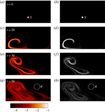
(a,c,e,g) Snapshots from the PDE simulation of the forward problem (2.1). The quantity contoured is
 $\log _{10}c(\boldsymbol{x},t)$
, for
 $t=0$
, 20, 30 and 50, with contour interval 0.5 (see greyscale/colour bar). (b,d, f,h) Scatterplot of
 $10^{4}$
solutions
 $\boldsymbol{X}_{t}$
of the SDE (3.1) at the same times.

The stochastic Lagrangian methods described below will be verified against a numerical PDE solution of (2.1). The numerical method is a standard spectral method, exploiting the fact that, taking the Fourier transform of (2.1), the complex amplitudes of each Fourier mode of
 $c$
satisfy an ordinary differential equation that is coupled only to its near neighbours in wavenumber space. High accuracy is possible once a resolution threshold is crossed, because the spectral power of
 $c$
drops off rapidly for wavenumbers
 $k\gtrsim {\it\kappa}^{-1/2}$
. The integrations used below, mainly at a resolution of
 $512\times 256$
wavenumbers, have been verified against a
 $1024\times 512$
calculation, with excellent agreement.
The specific initial condition
 $S(\boldsymbol{x})=\text{exp}(-|\boldsymbol{x}-\boldsymbol{x}_{s}|^{2}/2W_{s}^{2})$
, centred on
 $\boldsymbol{x}_{s}=({\rm\pi},{\rm\pi}/4)^{\dagger }$
and with horizontal scale
 $W_{s}=1/20\sqrt{2}$
, is applied at
 $t=0$
. Figure 1(a,c,e,g) shows snapshots of the developing PDE solution (note the logarithmic contour interval) at
 $t=0,20,30$
and
 $t=50=T$
, where
 $T$
is the receptor time, which corresponds to approximately five cycles of the periodic flow (2.3). The partial barrier to transport is evident in figure 1, because the tracer is stirred and mixed across the lower left of the domain, with little penetrating into the upper right. The receptor function, which is chosen to pick out a typical tracer filament (not visible in the
 $t=50$
panel in figure 1 as its concentration
 $c\lesssim 10^{-5}$
), is taken to be
 $R(\boldsymbol{x})=\exp (-|\boldsymbol{x}-\boldsymbol{x}_{r}|^{2}/2W_{r}^{2})$
with
 $\boldsymbol{x}_{r}=(4.35,2.05)^{\dagger }$
and
 $W_{r}=1/5\sqrt{2}$
(see the circle in the
 $t=50$
panel). Although concentrations in
 $\mathscr{R}$
are relatively low, the quantity
 $\mathscr{I}$
can be calculated to high accuracy by the PDE method (
 $\mathscr{I}=1.522583\times 10^{-7}$
to seven significant figures). The focus of all that follows is to develop efficient Lagrangian methods that can be used to estimate both
 $\mathscr{I}$
and the (weighted) distribution of tracer
 $c(\boldsymbol{x},T)R(\boldsymbol{x})$
throughout the receptor region at the end of the simulation.
2.2. The adjoint problem
In the Lagrangian methods to be described below, a central role is taken by the solution, or approximate solution, of the adjoint of (2.1) (sometimes the ‘retro-transport equation’ (e.g. Hourdin & Talagrand Reference Hourdin and Talagrand2006)), which provides an alternative means of obtaining
 $\mathscr{I}$
. A brief review is warranted. The retro-transport equation is obtained by first expressing (2.1) using the operator formalism,
 $$\begin{eqnarray}\mathscr{L}c=s,\end{eqnarray}$$
where
 $$\begin{eqnarray}\mathscr{L}\equiv \partial _{t}+(\boldsymbol{u}\boldsymbol{\cdot }\boldsymbol{{\rm\nabla}})-\boldsymbol{{\rm\nabla}}\boldsymbol{\cdot }({\bf\kappa}\boldsymbol{\cdot }\boldsymbol{{\rm\nabla}})\end{eqnarray}$$
is the forward linear transport operator. Next it is necessary to define an inner product for integrable functions
 $f(\boldsymbol{x},t)$
and
 $g(\boldsymbol{x},t)$
defined on
 $\mathscr{D}\times \mathbb{R}$
,
 $$\begin{eqnarray}\langle \,f,g\rangle =\int _{-\infty }^{\infty }\int _{\mathscr{D}}f(\boldsymbol{x},t)g(\boldsymbol{x},t)\text{d}\boldsymbol{x}\text{d}t.\end{eqnarray}$$
The inner product (2.7) can be used to define the adjoint
 $\mathscr{L}^{\dagger }$
of
 $\mathscr{L}$
, according to the usual definition
 $\langle \,f,\mathscr{L}^{\dagger }g\rangle =\langle \mathscr{L}f,g\rangle$
for all admissible
 $f$
and
 $g$
. It is a straightforward exercise in integration by parts to show that the adjoint transport operator satisfies
 $$\begin{eqnarray}\mathscr{L}^{\dagger }\equiv -\partial _{t}-(\boldsymbol{u}\boldsymbol{\cdot }\boldsymbol{{\rm\nabla}})-\boldsymbol{{\rm\nabla}}\boldsymbol{\cdot }({\bf\kappa}\boldsymbol{\cdot }\boldsymbol{{\rm\nabla}}).\end{eqnarray}$$
In terms of the inner product, the integral quantity (2.4) is given by
 $\mathscr{I}=\langle c,r\rangle$
. If we now define the retro-transport equation to be
 $$\begin{eqnarray}\mathscr{L}^{\dagger }c^{\ast }=r,\end{eqnarray}$$
then
 $\mathscr{I}$
can be manipulated as follows:
 $$\begin{eqnarray}\mathscr{I}=\langle c,r\rangle =\langle c,\mathscr{L}^{\dagger }c^{\ast }\rangle =\langle \mathscr{L}c,c^{\ast }\rangle =\langle s,c^{\ast }\rangle .\end{eqnarray}$$
In other words, rather than solving (2.1) to obtain
 $\mathscr{I}$
, an alternative is to solve (2.9) for
 $c^{\ast }$
, and then obtain
 $\mathscr{I}$
by evaluating the inner product with
 $s$
. It is clear from the sign of the diffusion term in
 $\mathscr{L}^{\dagger }$
that, for (2.9) to remain well posed, it must be solved backwards in time. In the case of our instantaneous receptor at
 $t=T$
, (2.9) takes initial conditions
 $c^{\ast }(\boldsymbol{x},T)=R(\boldsymbol{x})$
.
A formal interpretation of the adjoint solution
 $c^{\ast }(\boldsymbol{x},t)$
is that it denotes sensitivity of
 $\mathscr{I}$
with respect to a small change in the source
 $s$
at location
 $(\boldsymbol{x},t)$
, as can be expressed mathematically using the Fréchet derivative
 $c^{\ast }={\it\delta}\mathscr{I}/{\it\delta}s$
. Alternatively, a more physical interpretation is that
 $c^{\ast }$
is a measure of the quantity of fluid at a given point that will subsequently arrive at the receptor at time
 $t=T$
, weighted by
 $R(\boldsymbol{x})$
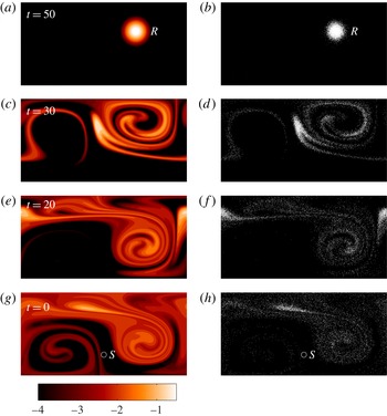
. Figure 2(a,c,e,g) shows snapshots from the PDE solution of (2.9) at times
 $t=50,30,20$
and 0. The transport barrier is again evident, as
 $c^{\ast }$
remains low in the lower left of the domain. The accuracy of the solution can be checked directly by recalculating
 $\mathscr{I}=\langle s,c^{\ast }\rangle$
. Agreement with the forward calculation (
 $\mathscr{I}\approx 1.522583\times 10^{-7}$
) is obtained to 11 significant figures, demonstrating the accuracy of the PDE algorithm.
(a,c,e,g) Snapshots from the PDE simulation of the forward problem (2.1). The quantity contoured is
 $\log _{10}c^{\ast }(\boldsymbol{x},t)$
, for
 $t=50$
, 30, 20 and 0, and with contour interval 0.5. (b,d, f,h) Scatterplot of
 $10^{4}$
solutions
 $\boldsymbol{X}_{{\it\tau}}$
of the SDE given by (3.1) again at
 ${\it\tau}=0$
, 20, 30 and 50 (equivalently
 $t=50$
, 30, 20 and 0).

2.3. The density of trajectories
A useful quantity is the product of the solutions of (2.1) and (2.9), i.e. the density of trajectories
 $D(\boldsymbol{x},t)=c(\boldsymbol{x},t)\,c^{\ast }(\boldsymbol{x},t)$
. Some intuition as to why
 $D$
is significant for importance sampling follows if one interprets
 $c(\boldsymbol{x},t)$
as (proportional to) the probability density of a trajectory originating in
 $\mathscr{S}$
at
 $t=0$
arriving at
 $\boldsymbol{x}$
at time
 $t$
. Then
 $c^{\ast }(\boldsymbol{x},t)$
is the analogous quantity measuring the probability of the trajectory at
 $(\boldsymbol{x},t)$
ending up in
 $\mathscr{R}$
at
 $t=T$
. The product
 $D(\boldsymbol{x},t)$
is therefore proportional to the probability of a trajectory passing through
 $(\boldsymbol{x},t)$
as it travels from
 $\mathscr{S}\rightarrow \mathscr{R}$
. Intuitively, an optimal Lagrangian algorithm for
 $\mathscr{S}\rightarrow \mathscr{R}$
transport should distribute trajectories in proportion to
 $D(\boldsymbol{x},t)$
, as will be demonstrated below.
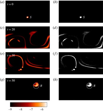
Figure 3(a,c,e,g) shows snapshots of
 $D(\boldsymbol{x},t)$
for our model problem. The
 $t=20$
and
 $t=30$
panels illustrate at a glance why we have described our problem as ‘hard’. The greater part of the
 $D(\boldsymbol{x},t)$
field is seen to occupy around 10 or so small and disjoint regions of the domain. An effective adaptive trajectory algorithm must sample each of these disjoint regions efficiently without wasting trajectories elsewhere.
(a,c,e,g) Snapshots of the density of trajectories
 $D(\boldsymbol{x},t)$
defined in § 2.3 and calculated from the numerical solutions of forward (2.1) and retro (2.9) PDEs. The quantity contoured is
 $\log _{10}(D(\boldsymbol{x},t))$
, for
 $t=0$
, 20, 30 and 50, and with contour interval 0.5. (b,d, f,h) Scatterplot of
 $10^{4}$
solutions
 $\boldsymbol{Y}_{t}$
of the SDE experiment CHEAT also at
 $t=0$
, 20, 30 and 50. CHEAT solves (3.7) with the correcting velocity
 $\boldsymbol{v}$
given by (3.18), as interpolated from the numerical solution of (2.9).

A property of
 $D(\boldsymbol{x},t)$
(e.g. Hourdin & Talagrand Reference Hourdin and Talagrand2006) is that, during times when the source function
 $s(\boldsymbol{x},t)$
and receptor function
 $r(\boldsymbol{x},t)$
are zero, its domain integral is constant. The divergence theorem in two dimensions can be used to show this, as follows:
 $$\begin{eqnarray}\displaystyle \frac{\text{d}}{\text{d}t}\int _{\mathscr{D}}D(\boldsymbol{x},t)\,\text{d}\boldsymbol{x} & = & \displaystyle \int _{\mathscr{D}}[c_{t}(\boldsymbol{x},t)c^{\ast }(\boldsymbol{x},t)+c(\boldsymbol{x},t)c_{t}^{\ast }(\boldsymbol{x},t)]\,\text{d}\boldsymbol{x}\nonumber\\ \displaystyle & = & \displaystyle \int _{\mathscr{D}}\{[-\boldsymbol{u}\boldsymbol{\cdot }\boldsymbol{{\rm\nabla}}c+\boldsymbol{{\rm\nabla}}\boldsymbol{\cdot }({\bf\kappa}\boldsymbol{\cdot }\boldsymbol{{\rm\nabla}}c)]c^{\ast }+c[-\boldsymbol{u}\boldsymbol{\cdot }\boldsymbol{{\rm\nabla}}c^{\ast }-\boldsymbol{{\rm\nabla}}\boldsymbol{\cdot }({\bf\kappa}\boldsymbol{\cdot }\boldsymbol{{\rm\nabla}}c^{\ast })]\}\text{d}\boldsymbol{x}\nonumber\\ \displaystyle & = & \displaystyle \int _{\mathscr{D}}\boldsymbol{{\rm\nabla}}\boldsymbol{\cdot }(\boldsymbol{u}cc^{\ast }+c^{\ast }{\bf\kappa}\boldsymbol{\cdot }\boldsymbol{{\rm\nabla}}c-c{\bf\kappa}\boldsymbol{\cdot }\boldsymbol{{\rm\nabla}}c^{\ast })\,\text{d}\boldsymbol{x}\nonumber\\ \displaystyle & = & \displaystyle \int _{\partial \mathscr{D}}[\boldsymbol{u}\boldsymbol{\cdot }\boldsymbol{n}cc^{\ast }+c^{\ast }(\boldsymbol{n}\boldsymbol{\cdot }{\bf\kappa}\boldsymbol{\cdot }\boldsymbol{{\rm\nabla}}c)-c(\boldsymbol{n}\boldsymbol{\cdot }{\bf\kappa}\boldsymbol{\cdot }\boldsymbol{{\rm\nabla}}c^{\ast })]\text{d}s=0,\end{eqnarray}$$
where
 $\boldsymbol{n}$
is the unit normal to
 $\partial \mathscr{D}$
. The final equality follows from there being no normal flow at the boundary
 $\partial \mathscr{D}$
(i.e.
 $\boldsymbol{u}\boldsymbol{\cdot }\boldsymbol{n}=0$
) and the no-flux boundary conditions (2.2) for
 $c$
and
 $c^{\ast }$
on
 $\partial \mathscr{D}$
.
For our problem it follows that
 $$\begin{eqnarray}\int _{\mathscr{D}}D(\boldsymbol{x},t)\,\text{d}\boldsymbol{x}=\mathscr{I}\quad \text{at all times}~t\in [0,T].\end{eqnarray}$$
3. Stochastic representations of the advection–diffusion problem
3.1. Direct and adjoint stochastic representations
The direct stochastic Lagrangian model corresponding to (2.1) consists of an Itô-type SDE for the particle position
 $\boldsymbol{X}_{t}$
. The SDE in question is chosen in order that the probability density
 $p(\boldsymbol{x},t)$
of the random variable
 $\boldsymbol{X}_{t}$
evolves in time according to a Fokker–Planck equation (sometimes forward Chapman–Kolmogorov equation) that is identical to (2.1). The method for deriving an SDE from a given Fokker–Planck PDE (or vice versa) is standard in stochastic calculus (e.g. section 4.3.4 of Gardiner Reference Gardiner2009). In the case of (2.1), the SDE is
 $$\begin{eqnarray}\text{d}\boldsymbol{X}_{t}=(\boldsymbol{u}(\boldsymbol{X}_{t},t)+\boldsymbol{{\rm\nabla}}\boldsymbol{\cdot }{\bf\kappa}(\boldsymbol{X}_{t},t))\,\text{d}t+(2{\bf\kappa})^{1/2}(\boldsymbol{X}_{t},t)\boldsymbol{\cdot }\text{d}\boldsymbol{W}_{t},\quad \boldsymbol{X}_{0}\sim S(\boldsymbol{x})/S_{00},\end{eqnarray}$$
where
 $\text{d}\boldsymbol{W}_{t}$
are the increments of a two-dimensional Brownian (Wiener) process, and the square root of a symmetric positive-definite tensor
 ${\bf\kappa}$
follows the standard definition. Notice that in (3.1) the probability density of the initial particle position
 $\boldsymbol{X}_{0}$
is specified to ensure
 $p(\boldsymbol{x},0)=S(\boldsymbol{x})/S_{00}$
(where the normalising constant
 $S_{00}$
is the domain integral of
 $S(\boldsymbol{x})$
). The consequence is that at subsequent times the respective distributions are in direct proportion, i.e.
 $p(\boldsymbol{x},t)=c(\boldsymbol{x},t)/S_{00}$
.
Figure 1(b,d,f,h) shows scatterplots of
 $\boldsymbol{X}_{t}$
for an ensemble of
 $N=10^{4}$
realisations of (3.1). Equation (3.1) is solved numerically using a suitable second-order Runge–Kutta time-stepping scheme for time-dependent SDEs (see Tocino & Ardanuy (Reference Tocino and Ardanuy2002) and note that their scheme simplifies considerably when the diffusivity is constant and isotropic). Note that the Tocino–Ardanuy scheme is ‘weak’ in the sense that it converges only in probability as step size is reduced, as opposed to being ‘strong’ in the sense of converging to individual sample paths of the stochastic process. It is weak convergence that is appropriate for the problem in hand. In comparison tests with the PDE solution, using the kernel density method described below, a time step of
 ${\it\delta}t=0.01$
was found to be adequate to ensure that the numerical error was significantly less than the statistical error when using
 $N=10^{6}$
particles. It is immediately evident in figure 1 that the distribution of
 $\boldsymbol{X}_{t}$
follows that of
 $c(\boldsymbol{x},t)$
as expected. It is equally apparent that exactly zero particles end up in the receptor region
 $\mathscr{R}$
(based on the PDE solution, the probability of a particle arriving in
 $\mathscr{R}$
at
 $T=50$
under (3.1) is about
 $2\times 10^{-5}$
). The integral
 $\mathscr{I}$
can be estimated from the stochastic process using
 $$\begin{eqnarray}\mathscr{I}=S_{00}\,\mathbb{E}(R(\boldsymbol{X}_{T}))=S_{00}\int _{\mathscr{D}}R(\boldsymbol{x})p(\boldsymbol{x},T)\,\text{d}\boldsymbol{x}=\langle c,r\rangle .\end{eqnarray}$$
Figure 1 makes clear, however, that efforts to calculate
 $\mathscr{I}$
by estimating the expectation in (3.2) will require very large ensembles. Estimators based on (3.2) are described as ‘high-variance’ estimators in the stochastic calculus literature, and efforts to improve them are called ‘variance reduction methods’ (e.g. Kloeden & Platen Reference Kloeden and Platen1992).
The same approach can be taken with the adjoint ‘retro-transport’ equation (2.9). Its stochastic representation is
 $$\begin{eqnarray}\text{d}\bar{\boldsymbol{X}}_{{\it\tau}}=(-\boldsymbol{u}(\bar{\boldsymbol{X}}_{{\it\tau}},{\it\tau})+\boldsymbol{{\rm\nabla}}\boldsymbol{\cdot }{\bf\kappa}(\bar{\boldsymbol{X}}_{{\it\tau}},{\it\tau}))\text{d}{\it\tau}+(2{\bf\kappa})^{1/2}(\bar{\boldsymbol{X}}_{{\it\tau}},{\it\tau})\boldsymbol{\cdot }\text{d}\boldsymbol{W}_{{\it\tau}},\quad \bar{\boldsymbol{X}}_{0}\sim R(\boldsymbol{x})/R_{00},\end{eqnarray}$$
where
 ${\it\tau}=T-t$
runs backwards in time, and
 $\mathscr{I}$
is obtained from
 $$\begin{eqnarray}\mathscr{I}=R_{00}\,\mathbb{E}(S(\bar{\boldsymbol{X}}_{{\it\tau}=T})).\end{eqnarray}$$
Figure 2(b,d, f,h) shows scatterplots of solutions of (3.3). The distribution of
 $\bar{\boldsymbol{X}}_{{\it\tau}=T-t}$
by design matches
 $c^{\ast }(\boldsymbol{x},t)$
.
Kernel density methods (e.g. Silverman Reference Silverman1986; Wand & Jones Reference Wand and Jones1994) can be used to estimate
 $c$
and
 $c^{\ast }$
from ensembles (e.g.
 $\boldsymbol{X}_{t}^{(i)},~i=1,\dots ,N$
) of solutions of (3.1) and (3.3), respectively. In terms of a symmetric kernel function
 $K(\boldsymbol{x})$
with unit integral and finite variance, suitable estimators are
 $$\begin{eqnarray}\left.\begin{array}{@{}l@{}}\displaystyle \bar{c}(\boldsymbol{x},t)=\frac{1}{Nh}\mathop{\sum }_{i=1}^{N}K\left(\frac{\boldsymbol{x}-\boldsymbol{X}_{t}^{(i)}}{h}\right)+\text{`image terms'},\\ \displaystyle \bar{c}^{\ast }(\boldsymbol{x},t)=\frac{1}{N^{\ast }h}\mathop{\sum }_{i=1}^{N^{\ast }}K\left(\frac{\boldsymbol{x}-\bar{\boldsymbol{X}}_{{\it\tau}=T-t}^{(i)}}{h}\right)+\text{`image terms'}.\end{array}\right\}\end{eqnarray}$$
Here
 $h$
is a (small) kernel bandwidth, and ‘image terms’ refer to contributions from the images of trajectories, introduced to satisfy the boundary conditions. Formally, there are an infinite number of images generated by repeated reflection in the boundaries at
 $y=0,{\rm\pi}$
, and located at periodic intervals of
 $2{\rm\pi}$
in
 $x$
. In practice, however, only the former need be considered and only for particles close to the boundaries. The accuracy of the estimate
 $\bar{c}^{\ast }$
of the adjoint solution will prove important in the construction of the Lagrangian estimators to be developed in § 4 below.
It is worth commenting that, if the kernel density estimates (3.5) are used to estimate
 $\mathscr{I}$
using the density of trajectories formula (2.12), the ‘forward–reverse’ representation of Milstein, Schoenmakers & Spokoiny (Reference Milstein, Schoenmakers and Spokoiny2004) is recovered as a straightforward consequence,
 $$\begin{eqnarray}\mathscr{I}\approx \int _{\mathscr{D}}\bar{c}(\boldsymbol{x},t)\bar{c}^{\ast }(\boldsymbol{x},t)\,\text{d}\boldsymbol{x}=\frac{1}{NN^{\ast }h}\mathop{\sum }_{i=1}^{N}\mathop{\sum }_{j=1}^{N^{\ast }}K^{(2)}\left(\frac{\boldsymbol{X}_{t}^{(i)}-\bar{\boldsymbol{X}}_{{\it\tau}=T-t}^{(j)}}{h}\right)+\text{`image terms'}.\end{eqnarray}$$
Here
 $K^{(2)}$
is a new kernel generated from the self-convolution of the original kernel
 $K$
(see e.g. p. 49 of Silverman Reference Silverman1986). In many practical circumstances, particularly where source and receptor regions
 $\mathscr{S}$
and
 $\mathscr{R}$
are spatially and temporally localised, the forward–reverse estimator will have lower variance. It is particularly useful when the Green’s function of the transport operator
 $\mathscr{L}$
(in the terminology of probability theory, the transition density) is sought (corresponding to source
 $\mathscr{S}$
and receptor
 $\mathscr{R}$
being points in
 $\mathscr{D}$
, for which case the estimator (3.2) has infinite variance). For non-localised
 $\mathscr{S}$
and
 $\mathscr{R}$
, the estimator (3.6) is biased, and converges more slowly with ensemble sizes
 $N$
and
 $N^{\ast }$
compared with the unbiased estimator (3.2). However, because it can have a much lower starting variance, it can often be of practical value (see e.g. the ocean transport modelling study of Spivakovskaya et al. (Reference Spivakovskaya, Heemink, Milstein and Schoenmakers2005)).
3.2. Importance sampling using Milstein’s measure transformation method
The measure transformation method of Milstein (Reference Milstein1995) is based on Girsanov’s theorem in stochastic calculus (e.g. Øksendal Reference Øksendal2007, chap. 8). Usually, Girsanov’s theorem is proved using results from measure theory, including the use of the Radon–Nikodym derivative, which may be unfamiliar to some applied mathematicians. Consequently, all of the results used here will be first proved using a relatively elementary (and, to the author’s knowledge, novel) PDE-based approach. The starting point of Milstein’s method is the extended stochastic process
 $$\begin{eqnarray}\left.\begin{array}{@{}l@{}}\text{d}\boldsymbol{Y}_{t}=(\boldsymbol{u}(\boldsymbol{Y}_{t},t)+\boldsymbol{v}(\boldsymbol{Y}_{t},t)+\boldsymbol{{\rm\nabla}}\boldsymbol{\cdot }{\bf\kappa}(\boldsymbol{Y}_{t},t))\,\text{d}t+(2{\bf\kappa})^{1/2}(\boldsymbol{Y}_{t},t)\boldsymbol{\cdot }\text{d}\boldsymbol{W}_{t},\\ \text{d}{\it\Theta}_{t}=-2^{-1/2}{\it\Theta}_{t}\,\boldsymbol{v}(\boldsymbol{Y}_{t},t)\boldsymbol{\cdot }{\bf\kappa}^{-1/2}(\boldsymbol{Y}_{t},t)\boldsymbol{\cdot }\text{d}\boldsymbol{W}_{t}.\end{array}\right\}\end{eqnarray}$$
It is to be emphasised that it is the same three-dimensional Brownian increment
 $\text{d}\boldsymbol{W}_{t}$
in each equation of (3.7). The initial conditions of (3.7), which must be consistent with the initial condition
 $c(\boldsymbol{x},0)=S(\boldsymbol{x})$
of (2.1), are in general given by
 $$\begin{eqnarray}\boldsymbol{Y}_{0}\sim g(\boldsymbol{x})S(\boldsymbol{x})/G_{00},\quad {\it\Theta}_{0}=G_{00}g(\boldsymbol{Y}_{\mathbf{0}})^{-1},\quad G_{00}=\int _{\mathscr{D}}g(\boldsymbol{x})S(\boldsymbol{x})\,\text{d}\boldsymbol{x}.\end{eqnarray}$$
In (3.7),
 $\boldsymbol{v}(\boldsymbol{x},t)$
is a smooth but otherwise arbitrary vector field defined everywhere in
 $\mathscr{D}$
; and similarly in (3.8),
 $g(\boldsymbol{x})$
is a smooth function in
 $\mathscr{D}$
. Evidently, the particle trajectories
 $\boldsymbol{Y}_{t}$
in (3.7) differ from those of (3.1) in that they are advected by the corrected velocity field
 $\boldsymbol{u}+\boldsymbol{v}$
instead of by
 $\boldsymbol{u}$
. There is also an additional equation for a stochastic variable
 ${\it\Theta}_{t}$
coupled to the trajectory equation. The key result obtained from Girsanov’s theorem (following e.g. Kloeden & Platen Reference Kloeden and Platen1992) is that, for any choice of
 $\boldsymbol{v}$
and
 $g$
, the process (3.7) satisfies
 $$\begin{eqnarray}\mathscr{I}=\mathbb{E}({\it\Theta}_{T}R(\boldsymbol{Y}_{T})).\end{eqnarray}$$
The result (3.9) will be established below using a PDE method. Note that the original direct estimate (3.2) is recovered under the choice
 $\boldsymbol{v}=0$
,
 $g=1$
. Note also that, in order to frame our discussion in terms of ‘correcting velocities’, a form of the result has been given that is valid only when the diffusivity tensor
 ${\bf\kappa}$
is everywhere strictly positive definite, and thus invertible. In the more general situation in which one or more eigenvalues of
 ${\bf\kappa}$
is(are) sometimes zero, care must be taken to restrict
 $\boldsymbol{v}$
to the direction of the eigenvector(s) of
 ${\bf\kappa}$
associated with its non-zero eigenvalue(s).
The aim of Milstein’s method is to choose
 $\boldsymbol{v}$
and
 $g$
judiciously in order that (3.9) is a ‘lower-variance’ estimator of
 $\mathscr{I}$
compared with (3.2). The variable
 ${\it\Theta}_{t}$
can be understood as a trajectory ‘weight’, which is constant in the uncorrected process (3.1), but is here allowed to evolve. Under a particular choice of
 $\boldsymbol{v}$
, the system (3.7) samples trajectories that, though (possibly) important for the problem of interest, may be highly improbable under the direct process (3.1). The trajectory weight
 ${\it\Theta}_{t}$
is designed to keep track of exactly how improbable the sampled trajectories are, essentially by integrating the relative probabilities of stochastic increments in the corrected versus the uncorrected process.
The result (3.9) can be established as follows. First, consider (3.7) as a three-dimensional vector-valued stochastic process, i.e. for
 $\boldsymbol{Z}_{t}=(Y_{1t}\;Y_{2t}\;{\it\Theta}_{t})^{\dagger }$
. The Fokker–Planck equation for the joint probability density
 $p(\boldsymbol{y},{\it\theta},t)$
for
 $\boldsymbol{Z}_{t}$
is then obtained as
 $$\begin{eqnarray}p_{t}+\boldsymbol{{\rm\nabla}}\boldsymbol{\cdot }((\boldsymbol{u}+\boldsymbol{v})p)-\boldsymbol{{\rm\nabla}}\boldsymbol{\cdot }({\bf\kappa}\boldsymbol{\cdot }\boldsymbol{{\rm\nabla}}p)+\boldsymbol{{\rm\nabla}}\boldsymbol{\cdot }(\boldsymbol{v}({\it\theta}p)_{{\it\theta}})-{\textstyle \frac{1}{4}}(\boldsymbol{v}\boldsymbol{\cdot }{\bf\kappa}^{-1}\boldsymbol{\cdot }\boldsymbol{v})({\it\theta}^{2}p)_{{\it\theta}{\it\theta}}=0,\end{eqnarray}$$
where
 $\boldsymbol{{\rm\nabla}}\equiv \boldsymbol{{\rm\nabla}}_{\boldsymbol{y}}$
acts on the spatial variable
 $\boldsymbol{y}$
only. Next consider the integrated quantity
 $$\begin{eqnarray}P(\boldsymbol{y},t)=\int _{0}^{\infty }{\it\theta}p(\boldsymbol{y},{\it\theta},t)\text{d}{\it\theta}.\end{eqnarray}$$
Multiplying (3.10) by
 ${\it\theta}$
and then integrating leads to (following some integration by parts)
 $$\begin{eqnarray}\partial _{t}P+\boldsymbol{{\rm\nabla}}\boldsymbol{\cdot }(\boldsymbol{u}P)-\boldsymbol{{\rm\nabla}}\boldsymbol{\cdot }({\bf\kappa}\boldsymbol{\cdot }\boldsymbol{{\rm\nabla}}P)=0.\end{eqnarray}$$
In other words (since here
 $\boldsymbol{{\rm\nabla}}\boldsymbol{\cdot }\boldsymbol{u}=0$
),
 $P$
satisfies our original advection–diffusion equation (2.1). Noting that the SDE initial condition (3.8) corresponds to
 $p(\boldsymbol{y},{\it\theta},0)={\it\delta}({\it\theta}-G_{00}g(\boldsymbol{y})^{-1})g(\boldsymbol{y})S(\boldsymbol{x})/G_{00}$
, it follows that the correct initial condition for (3.12), i.e.
 $P(\boldsymbol{y},0)=S(\boldsymbol{x})$
, also holds. Consequently
 $$\begin{eqnarray}P(\boldsymbol{y},t)=c(\boldsymbol{y},t)\end{eqnarray}$$
at subsequent times
 $t$
. The result (3.9) then follows from the definition of expectation:
 $$\begin{eqnarray}\mathbb{E}({\it\Theta}_{T}R(\boldsymbol{Y}_{T}))=\int _{\mathscr{D}}\int _{0}^{\infty }{\it\theta}R(\boldsymbol{y})p(\boldsymbol{y},{\it\theta},T)\text{d}{\it\theta}\text{d}\boldsymbol{y}=\int _{\mathscr{ D}}R(\boldsymbol{y})P(\boldsymbol{y},T)\,\text{d}\boldsymbol{y}=\langle c,r\rangle =\mathscr{I}.\end{eqnarray}$$
The fact that the PDE analogue of Girsanov’s theorem/Milstein’s method involves solving a PDE (3.10) in a higher-dimensional space than the original perhaps explains why the approach has not previously been exploited in the context of PDE methods for advection–diffusion problems. The great advantage of the stochastic representation is that the extra dimension can be accommodated at little extra cost.
The key question remains how to choose
 $\boldsymbol{v}$
in (3.7) and
 $g$
in (3.8). This is a more delicate matter than might be supposed, as the following two examples will demonstrate.
3.3. Milstein’s method with a uniform correcting velocity
Some intuition about the consequences of a poor choice of the correcting velocity
 $\boldsymbol{v}$
follows from setting
 $\boldsymbol{v}=V\boldsymbol{i}$
, where
 $V$
is a constant and
 $\boldsymbol{i}$
is the unit vector in the
 $x$
direction, together with
 $g(\boldsymbol{x})=1$
. For the case of the constant and isotropic diffusivity problem under consideration, the trajectory weight (3.7) can be integrated explicitly to give
 $$\begin{eqnarray}{\it\Theta}_{t}={\it\Theta}_{0}\exp \left(-\frac{V^{2}t}{4{\it\kappa}}+\frac{VW_{1t}}{(2{\it\kappa})^{1/2}}\right),\end{eqnarray}$$
where
 $W_{1t}$
is the
 $x$
component of the vector-valued Wiener process
 $\boldsymbol{W}_{t}$
. It follows that the random variable
 ${\it\Theta}_{t}/{\it\Theta}_{0}$
has probability density
 $$\begin{eqnarray}{\it\rho}({\it\theta})=\frac{1}{({\rm\pi}t_{\ast })^{1/2}{\it\theta}}\exp \left(-\frac{(\log {\it\theta}+{\textstyle \frac{1}{4}}t_{\ast })^{2}}{t_{\ast }}\right),\quad t_{\ast }=\frac{V^{2}t}{{\it\kappa}}.\end{eqnarray}$$
The distribution
 ${\it\rho}({\it\theta})$
has a very long tail for
 $t_{\ast }\gg 1$
. It follows that, after sufficient time, the estimator (3.9) will necessarily have very high variance, making it a poor estimator of
 $\mathscr{I}$
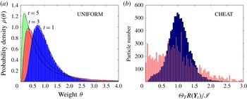
. By way of illustration, figure 4(a,b) shows the evolution of the distribution (3.16) at
 $t_{\ast }=0.5$
, 1.5 and 2.5. The results are compared to histograms of
 ${\it\Theta}_{t}$
at corresponding times
 $t=1$
, 3 and 5 in a numerical integration of (3.7), with
 $V=0.01$
(recall that
 ${\it\kappa}=2\times 10^{-4}$
). Even though the correcting velocity
 $V=0.01$
is so small that it is difficult to distinguish by eye between corrected and uncorrected particle distributions (not shown), it is obvious that the variance of
 ${\it\Theta}_{t}$
is already alarmingly high after only 10 % of the total integration time.
(a) Normalised histograms of trajectory weight
 ${\it\Theta}_{t}$
in the UNIFORM correcting velocity experiment with
 $V=0.01$
at times
 $t=1$
(dark grey, blue online), 3 (grey, red online) and 5 (light grey, green online), versus the corresponding analytic solutions (curves) given by (3.16). (b) Histograms of
 ${\it\Theta}_{T}R(\boldsymbol{Y}_{t})/\mathscr{I}$
in the CHEAT experiments described in the text. Dark grey (blue online) histogram, interpolation time
 ${\rm\Delta}t=0.1$
; light grey (red online) histogram
 ${\rm\Delta}t=0.2$
.

To make the above observations more precise, a lower bound can be derived for the variance of the random variable
 ${\it\Pi}\equiv {\it\Theta}_{T}R(\boldsymbol{Y}_{T})$
. Exploiting the facts that
 $\mathbb{E}({\it\Pi})=\mathscr{I}$
(from (3.14)), that
 $R(\boldsymbol{x})$
is bounded and that the distribution of
 ${\it\Theta}_{T}$
is given by (3.16) with
 $t_{\ast }=V^{2}T/{\it\kappa}$
, it is shown in appendix A that
 $$\begin{eqnarray}\text{Var}({\it\Pi})\geqslant X(t_{\ast },\mathscr{I})S_{00}\mathscr{I}-\mathscr{I}^{2},\end{eqnarray}$$
where
 $X(t_{\ast },\mathscr{I})$
is a function that, for fixed
 $\mathscr{I}>0$
, can be shown at large
 $t_{\ast }$
to grow exponentially. For problems with fixed
 ${\it\kappa}$
and
 $T$
, as here, the inequality (3.17) allows an upper bound for
 $V$
to be calculated, beyond which
 $\text{Var}({\it\Pi})$
will certainly exceed the variance of the original estimator
 $\text{Var}(S_{00}R(\boldsymbol{X}_{T}))$
. For the problem at hand (with
 $T=50$
,
 ${\it\kappa}=2\times 10^{-4}$
,
 $\mathscr{I}\approx 1.52\times 10^{-7}$
and
 $S_{00}\approx 7.85\times 10^{-3}$
), the bound obtained is rather low,
 $|V|<0.03$
. As above, a correcting velocity
 $V$
of this magnitude has a very modest impact on the distribution of particles, making it clear that a naive application of Milstein’s method with a uniform correcting velocity is worse than useless for our problem.
The broader significance of this result is that it gives an explicit demonstration that, unless
 $\boldsymbol{v}$
is chosen with great care, the variance of
 ${\it\Theta}_{t}$
will grow and overwhelm any possible reduction in variance obtained from directing more particles into the receptor region
 $\mathscr{R}$
. In fact, as will be demonstrated next for the problem under consideration, great care is necessary in the choice of
 $\boldsymbol{v}$
to result in any variance reduction at all.
3.4. Milstein’s method with the optimal correcting velocity
Kloeden & Platen (Reference Kloeden and Platen1992) comment that, in principle, a ‘zero-variance’ estimator for
 $\mathscr{I}$
, i.e. an optimal importance sampling strategy, can be constructed by setting
 $\boldsymbol{v}=\boldsymbol{v}^{\ast }$
, where
 $\boldsymbol{v}^{\ast }$
is an ideal correcting velocity given by
 $$\begin{eqnarray}\boldsymbol{v}^{\ast }=2{c^{\ast }}^{-1}{\bf\kappa}\boldsymbol{\cdot }\boldsymbol{{\rm\nabla}}c^{\ast }.\end{eqnarray}$$
Here
 $c^{\ast }$
is the solution of the retro-transport (adjoint) equation (2.9). The standard proof for this is given in appendix B, where it is shown that the corresponding optimal choice in (3.8) is
 $g(\boldsymbol{x})=c^{\ast }(\boldsymbol{x},0)$
. Of course, the expression (3.18) cannot be used directly to construct a purely Lagrangian estimator, because it requires knowledge of
 $c^{\ast }$
, from which
 $\mathscr{I}$
can in any case be obtained directly using (2.10). Nevertheless, investigating solutions of the SDE system (3.7) with
 $\boldsymbol{v}=\boldsymbol{v}^{\ast }$
is instructive, both in providing intuition about how the ‘perfect’ importance sampling Lagrangian solution behaves, and as a test of the numerical implementation of (3.7).
Some results regarding the optimal importance sampling strategy follow from the observation that, when
 $\boldsymbol{v}=\boldsymbol{v}^{\ast }$
and
 $g(\boldsymbol{x})=c^{\ast }(\boldsymbol{x},0)$
, the Fokker–Planck equation (3.10) has the exact solution
 $$\begin{eqnarray}p(\boldsymbol{y},{\it\theta},t)={\it\delta}({\it\theta}-\mathscr{I}c^{\ast }(\boldsymbol{y},t)^{-1})\,c^{\ast }(\boldsymbol{y},t)\,c(\boldsymbol{y},t)\,\mathscr{I}^{-1}.\end{eqnarray}$$
The result (3.19) can be verified by the straightforward, if tedious, process of insertion in (3.10), provided that care is taken over the properties of generalised functions, i.e. the Dirac delta and its derivatives. That (3.19) is correctly normalised follows from (2.12). The solution (3.19) reveals the following:
-
(a) In the optimal importance sampling strategy, the distribution of particles in the domain is given by
(3.20)In other words, Lagrangian particles are distributed according to the density of trajectories defined in § 2.3. (Note that this result can also be obtained, avoiding the use of generalised functions, by first integrating (3.10) with respect to $$\begin{eqnarray}\bar{p}(\boldsymbol{y},t)=\int _{0}^{\infty }p(\boldsymbol{y},{\it\theta},t)\,\text{d}{\it\theta}=D(\boldsymbol{y},t)\,\mathscr{I}^{-1}.\end{eqnarray}$$
${\it\theta}$
to obtain an equation for
$\bar{p}$
.)
-
(b) In the optimal importance sampling strategy, the trajectory weights are everywhere inversely proportional to the local value of the adjoint solution, i.e.
${\it\Theta}_{t}\sim c^{\ast }(\boldsymbol{Y}_{t},t)^{-1}$
.


The results (a) and (b) show that the optimal strategy for Milstein’s method, i.e. with
 $\boldsymbol{v}=\boldsymbol{v}^{\ast }$
, is exactly consistent with the intuitive description of the importance of
 $D$
given in § 2.3. This intuition will be the basis of the purely Lagrangian strategies developed to estimate
 $\mathscr{I}$
in § 4 below, including the means to choose ‘winners’ in the GWTW algorithm to be discussed next.
Equation (3.7) has been solved numerically using a correcting velocity
 $\boldsymbol{v}=\boldsymbol{v}^{\ast }$
obtained from numerical interpolation of the Eulerian solution of (2.9) described in § 2.2 and shown in figure 2. The aim of this numerical experiment, named ‘CHEAT’ because the Eulerian solution that is being exploited can obviously be used to obtain
 $\mathscr{I}$
independently, is to check the results above and to gain some insight into their practical limitations. In the main experiment, cubic interpolation is used from the
 $1024\times 512$
gridded Eulerian solution, with linear interpolation in time between outputs at intervals
 ${\rm\Delta}t=0.1$
.
The particle positions for an ensemble of
 $N=10^{4}$
realisations of CHEAT are shown in figure 3(b,d, f,h). It is clear from figure 3 that the distribution of particles in CHEAT closely follows
 $D$
as predicted by (3.20). The trajectory weights, however, deviate from the prediction (b). Figure 4(b) shows a histogram (dark grey, blue online) of
 ${\it\Theta}_{T}R(\boldsymbol{Y}_{T})/\mathscr{I}$
for CHEAT. If
 $\boldsymbol{v}^{\ast }$
were exact (and the numerics were perfect), then
 ${\it\Theta}_{T}R(\boldsymbol{Y}_{T})/\mathscr{I}$
would be equal to unity. It is seen, however, to deviate substantially from this deterministic ideal. The main source of error is found to come from the linear interpolation in time between the calculated
 $\boldsymbol{v}^{\ast }$
fields, which are stored at discrete time intervals
 ${\rm\Delta}t=0.1$
. Evidence comes from a test in which
 ${\rm\Delta}t$
is increased to 0.2 (light grey histogram, red online), which shows a large increase in the standard deviation of
 ${\it\Theta}_{T}R(\boldsymbol{Y}_{T})/\mathscr{I}$
.
The sensitivity of the CHEAT results to
 ${\rm\Delta}t$
is illustrative of a major practical difficulty with Milstein’s method. Even relatively small errors in
 $\boldsymbol{v}^{\ast }$
cumulatively lead to large increases in the variance of the Lagrangian estimator. This finding influences our approach in § 4 below.
3.5. Grassberger’s GWTW branching process
An alternative to Milstein’s method is the GWTW importance sampling strategy (Grassberger Reference Grassberger1997, Reference Grassberger2002). GWTW is a branching process which in its simplest form is applied at discrete intervals
 ${\rm\Delta}t$
in time. Trajectories are first assigned an initial position and weight
 ${\it\Theta}_{0}$
, according to (3.8), exactly as for Milstein’s method. An ensemble of
 $N$
realisations of the direct SDE (3.1) is then integrated forwards from
 $t=0$
, with each member of the ensemble having weight
 ${\it\Theta}_{0}$
. However, in contrast to Milstein’s method, in GWTW trajectory weights
 ${\it\Theta}_{t}$
are updated only at discrete times
 $t=t_{j}$
(
 $t_{j}=j{\rm\Delta}t$
), instead of continuously in time. Nevertheless, the weight
 ${\it\Theta}_{t}$
performs exactly the same function for each algorithm.
At each branching time
 $t_{j}=j{\rm\Delta}t$
(
 $j=1,2,3,\dots$
), our implementation of the algorithm proceeds as follows:
-
(a) A scoring algorithm (see below) is used to assign each trajectory in the ensemble a score
$S_{t_{j}}^{(i)}~(i=1,\dots ,N)$
. The trajectories are then sorted into order of decreasing score. -
(b) The trajectories with the lowest scores are then considered sequentially. The trajectory with the
$m$
th lowest score is designated as a ‘loser’ if its score is less than one-third of the score of the trajectory with the
$m$
th highest score. The total number of losers found is denoted
$L$
. -
(c) The weights of the
$L$
loser trajectories are then randomly, with probability one-half, either doubled
${\it\Theta}_{t_{j}}\rightarrow 2{\it\Theta}_{t_{j}}$
or set to zero. The
$W~({\approx}L/2)$
trajectories with score zero are then removed from the calculation. -
(d) The
$W$
trajectories with the highest scores, designated as the ‘winners’, are then split into two trajectories, each with half the weight of its parent, i.e.
${\it\Theta}_{t_{j}}/2$
.


The steps (a)–(d) act to reduce the variance of the distribution of scores
 $\{S_{t_{j}}^{(i)},\;i=1,\dots ,N\}$
at each branching time. This variance reduction occurs because any trajectory with a score less than around half of the ensemble mean score will be identified as a loser, and will either have its score doubled or will be removed completely. Any trajectory with a score much greater than two or three times the ensemble mean will be identified as a winner, and will be reproduced, with each daughter trajectory having half its score. Provided that steps (a)–(d) are implemented sufficiently frequently in time, the net effect is to keep all scores within a factor of two or so of the ensemble mean. Crucially, this is achieved without changing either the number of trajectories or the overall expectation of the process.
The effectiveness of GWTW evidently depends upon the selection of an appropriate score
 $S_{t_{j}}$
for each trajectory, together with the choice of
 $g(\boldsymbol{x})$
in the initial condition (3.8). There is a clear analogy between choosing
 $S_{t_{j}}$
and choosing the correcting velocity
 $\boldsymbol{v}$
in Milstein’s method. Just as with Milstein’s method, we have found that a poor choice leads to poor performance. Based on the above, the ideal choice can be guided by result (b) in § 3.4, which gives the trajectory weights in the ‘perfect’ implementation of Milstein’s method. If the ideal score at time
 $t$
is taken to be the product of the trajectory weight and the local value of the adjoint solution, i.e.
 $$\begin{eqnarray}S_{t}={\it\Theta}_{t}\,c^{\ast }(\boldsymbol{X}_{t},t),\end{eqnarray}$$
then, based on the arguments given above, the GWTW algorithm will ensure that the distribution of values of
 $S_{t}$
will remain within a factor of two or so of the ensemble mean
 $\langle S_{t}\rangle$
. Hence the trajectory weights will satisfy
 $(\langle S_{t}\rangle c^{\ast }(\boldsymbol{X}_{t},t)^{-1})/2\lesssim {\it\Theta}_{t}\lesssim 2\langle S_{t}\rangle c^{\ast }(\boldsymbol{X}_{t},t)^{-1}$
, i.e. at any instant in time
 ${\it\Theta}_{t}$
is approximately inversely proportional to
 $c^{\ast }$
, as it is in the ideal implementation of Milstein’s method. Of course, as with Milstein’s method, the exact field
 $c^{\ast }$
is not available, but the result (3.21) will nevertheless guide our practical implementation of GWTW described in § 4.2 below.
4. Adaptive Lagrangian estimators for
$\mathscr{S}\rightarrow \mathscr{R}$
transport

Motivated by the above analysis, we proceed by considering forward estimators of
 $\mathscr{I}$
in which importance sampling is controlled by an estimate of the adjoint solution
 $c^{\ast }$
, which is generated from a preliminary ensemble of integrations of the retro-transport SDE (3.3). Much depends on the quality of the estimate
 $\bar{c}^{\ast }$
of
 $c^{\ast }$
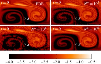
, of which some illustrative examples generated using the kernel density method are shown in figure 5.
Solution
 $c^{\ast }(\boldsymbol{x},0)$
of the retro-transport equation (2.9) versus kernel density reconstructions
 $\bar{c}^{\ast }(\boldsymbol{x},0)$
from ensembles of solutions of (3.3) with
 $N=10^{4}$
,
 $10^{5}$
and
 $10^{6}$
trajectories, respectively. The Gaussian kernel widths
 $h=0.015$
,
 $h=0.02$
and
 $h=0.04$
are used, which are close to the optimum value in each case.

Alternative approaches are possible. For example, Vanden-Eijnden & Weare (Reference Vanden-Eijnden and Weare2012) describe how results from large-deviation theory can be used to obtain an estimate of
 $\boldsymbol{v}^{\ast }$
for Milstein’s method that is asymptotically exact in the limit of small noise. To do this, it is necessary solve a variational problem for each trajectory at regular time intervals, with this problem being posed on the time interval
 $[t,T]$
. Our efforts to use this method for our model problem have not been successful for reasons to be given below.
The restriction here to forward estimators is simply to focus the discussion. Indeed, because both forward and backward trajectories are used, each of our approaches can be straightforwardly adapted to exploit the forward–reverse representation of Milstein et al. (Reference Milstein, Schoenmakers and Spokoiny2004) (see (3.6) above), which may lead to significant further improvements, particularly for very localised sources and receptors.
4.1. Estimators based on Milstein’s measure transformation method
A purely Lagrangian forward estimator for
 $\mathscr{I}$
can be created using the following four-stage algorithm:
-
(a) Generate an ensemble, of size
$N^{\ast }$
, of solutions of the retro-transport SDE (3.3). -
(b) Use the kernel density method (3.5) to generate a gridded estimate
$\bar{c}^{\ast }$
at time intervals
${\rm\Delta}t$
of the retro-transport solution
$c^{\ast }$
of (2.9), using the back trajectory ensemble. -
(c) Use the field
$\bar{c}^{\ast }$
to generate a correcting velocity
$\bar{\boldsymbol{v}}^{\ast }$
based on (3.18). This is multiplied by a smoothed step function
$F_{{\it\epsilon}}(\cdot )$
designed to smoothly reduce
$\bar{\boldsymbol{v}}^{\ast }$
to near zero in regions where
$\bar{c}^{\ast }$
is low, i.e. (4.1)Here
$$\begin{eqnarray}\bar{\boldsymbol{v}}^{\ast }=2F_{{\it\epsilon}}(\bar{c}^{\ast })\,\bar{c}^{\ast -1}{\bf\kappa}\boldsymbol{\cdot }\boldsymbol{{\rm\nabla}}\bar{c}^{\ast }.\end{eqnarray}$$
$F_{{\it\epsilon}}(x)$
approaches unity for
$x\gg {\it\epsilon}$
and decays monotonically and rapidly to zero for
$x\ll {\it\epsilon}$
(below,
$F_{{\it\epsilon}}(x)=\exp (-8(\log x/\log {\it\epsilon})^{12})$
is used).
-
(d) Solve (3.7) using correcting velocity
$\boldsymbol{v}=\bar{\boldsymbol{v}}^{\ast }$
from (4.1), using initial conditions (3.8), where the function
$g(\boldsymbol{x})={\it\epsilon}+\bar{c}^{\ast }(\boldsymbol{x},0)$
. This particular choice for
$g(\boldsymbol{x})$
is consistent with trusting the estimate
$\bar{c}^{\ast }$
to be a reasonable approximation for
$c^{\ast }$
only in regions where
$\bar{c}^{\ast }\gtrsim {\it\epsilon}$
.


The algorithm above requires the selection of a large number of numerical parameters (e.g. retro-ensemble size
 $N^{\ast }$
, kernel size
 $h$
, grid spacing
 ${\rm\Delta}x$
, time interval
 ${\rm\Delta}t$
, etc.), in addition to those associated with the SDE solutions themselves (e.g. time step), and the choice of the function
 $F_{{\it\epsilon}}(\cdot )$
. A complete numerical analysis and optimisation is therefore a formidable task, which we do not attempt here. Instead, we focus on the key, and not immediately transparent, role of the parameter
 ${\it\epsilon}$
. The reason that a finite
 ${\it\epsilon}$
is required is that Milstein’s method will fail whenever the trajectory passes through regions where the estimate
 $\bar{\boldsymbol{v}}^{\ast }$
differs significantly from the ideal
 $\boldsymbol{v}^{\ast }$
. The failure can be explained by analogy with the ‘uniform correcting velocity’ problem of § 3.3, which showed that the increase in
 $\text{Var}({\it\Theta}_{t})$
due to a poorly directed correcting velocity can rapidly overwhelm any variance reduction due to redirecting trajectories into the region of interest.
In our problem, the estimate
 $\bar{\boldsymbol{v}}^{\ast }$
is poor where there are few adjoint trajectories contributing to
 $\bar{c}^{\ast }$
, i.e. in all regions where
 $\bar{c}^{\ast }$
is small, and it turns out to be effective to set the correcting velocity
 $\boldsymbol{v}$
to be zero in these regions. It seems that such a fix will be necessary regardless of the method used to estimate
 $\bar{c}^{\ast }$
, because the relative error in
 $\bar{c}^{\ast }$
, which controls
 $\bar{\boldsymbol{v}}^{\ast }$
, will inevitably be higher where
 $\bar{c}^{\ast }$
is low. The smoothed step function in (4.1) acts to suppress
 $\bar{\boldsymbol{v}}^{\ast }$
everywhere that
 $\bar{c}^{\ast }\lesssim {\it\epsilon}$
. Broadly speaking, it turns out to be important to choose
 ${\it\epsilon}$
to be sufficiently large so that the estimate (4.1) is accurate throughout the region with
 $c^{\ast }\gtrsim {\it\epsilon}$
. It will be seen below that the algorithm is not sensitive to the precise value of
 ${\it\epsilon}$
, with near optimal results obtained provided
 ${\it\epsilon}$
is within an order of magnitude or so of its optimal value.
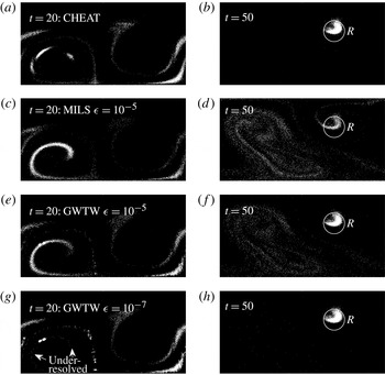
Figure 6 shows the trajectory positions at
 $t=20$
and
 $t=50$
in the CHEAT experiment and in Milstein’s method with
 $N^{\ast }=10^{5}$
and
 ${\it\epsilon}=10^{-5}$
. In the CHEAT experiment, trajectories are distributed almost exactly according to
 $D(\boldsymbol{x},t)$
, so CHEAT serves here as a reference that allows us to determine easily where the other methods are over- and under-resolved in terms of their distribution of particles. It can be seen in the
 $t=20$
panel that Milstein’s method integration with
 ${\it\epsilon}=10^{-5}$
maintains some resolution in all relevant regions, but is over-resolved where
 $c(\boldsymbol{x},t)$
is relatively large (compare figure 1) and somewhat under-resolved elsewhere. The distributions of trajectories for runs with other values of
 ${\it\epsilon}$
(not shown) are similar, but with fewer particles reaching
 $\mathscr{R}$
as
 ${\it\epsilon}$
is increased. It appears from figure 6 that the errors in Milstein’s method primarily stem not from a failure to simulate some of the
 $\mathscr{S}\rightarrow \mathscr{R}$
transport pathways, but from the excess variance in
 ${\it\Theta}_{T}$
introduced due to errors in
 $\boldsymbol{v}^{\ast }$
, as discussed in §§ 3.3 and 3.4 above. Because
 $\text{Var}({\it\Theta}_{T})$
decreases as
 ${\it\epsilon}$
is increased, there is an optimal value of
 ${\it\epsilon}$
for which sufficient trajectories reach
 $\mathscr{R}$
with
 $\text{Var}({\it\Theta}_{T})$
not too large, and this optimal value depends on the details of the problem.
Trajectory distributions at
 $t=20$
(a,c,e,g) and
 $t=50$
(b,d, f,h) in (a,b) the experiment CHEAT described in § 3.4, (c,d) Milstein’s method with
 $N^{\ast }=10^{5}$
and
 ${\it\epsilon}=10^{-5}$
, (e, f) GWTW with
 $N^{\ast }=10^{5}$
and
 ${\it\epsilon}=10^{-5}$
and (g,h) GWTW with
 $N^{\ast }=10^{5}$
and
 ${\it\epsilon}=10^{-7}$
.

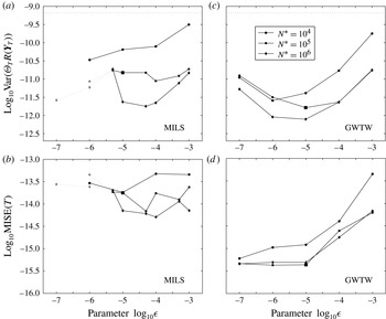
To quantify the influence of the quality of the estimate of
 $\bar{c}^{\ast }$
and the selection of
 ${\it\epsilon}$
, figure 7(a) shows calculated variances of the Lagrangian estimators, i.e.
 $\text{Var}({\it\Theta}_{T}R(\boldsymbol{Y}_{T}))$
. The variance of the direct estimator (i.e.
 $\text{Var}(S_{00}R(\boldsymbol{X}_{T}))$
), calculated directly from the PDE solution, is marked by the dotted line. The results are plotted as a function of
 ${\it\epsilon}$
, and are given for the three kernel density reconstructions of
 $\bar{c}^{\ast }$
, for
 $N^{\ast }=10^{4}$
,
 $10^{5}$
and
 $10^{6}$
, as shown in figure 5. The variance in each case is calculated from a forward ensemble of size
 $N=10^{5}$
, using the standard statistical estimator. A difficulty is that the random variable
 ${\it\Theta}_{T}R(\boldsymbol{Y}_{T})$
becomes long-tailed for calculations with
 ${\it\epsilon}=10^{-6}$
or smaller, and in these case the values obtained for the variance are likely to be underestimates due to poor sampling of the tail. Points for which the error in the sample mean, compared to the expected value
 $\mathscr{I}$
, is greater than the calculated value of
 $3(\text{Var}({\it\Theta}_{T}R(\boldsymbol{Y}_{T}))/N)^{1/2}$
(i.e. three standard deviations) are highlighted as being inconsistent and are consequently marked in grey. If these points are ignored, the results show that between one and two orders of magnitude of variance reduction is possible, and confirm that performance improves with increasing
 $N^{\ast }$
as is expected. The optimal value for
 ${\it\epsilon}$
is seen to be in the range
 $10^{-4}{-}10^{-5}$
.
(a,c) Calculated variance of the estimator
 ${\it\Theta}_{T}R(\boldsymbol{Y}_{T})$
, as a function of
 ${\it\epsilon}$
, for calculations using estimates of
 $\bar{c}^{\ast }$
based on
 $N^{\ast }=10^{4},10^{5}$
and
 $10^{6}$
trajectories: (a) Milstein’s method; (c) go-with-the-winners. Points for which the calculated variance is inconsistent with the error in the sample mean are shown in grey. The variance of the direct estimator is indicated by the dotted line in each panel. (b,d) As above, but showing
 $\text{MISE}(T)$
(4.2) for the same calculations.

An alternative measure of the accuracy of the calculations is given by the mean integrated square error (MISE) of the reconstructions of the tracer field within
 $\mathscr{R}$
. Here MISE is defined to be
 $$\begin{eqnarray}\text{MISE}(t)=\int _{\mathscr{D}}(c(\boldsymbol{x},t)-\bar{c}(\boldsymbol{x},t))^{2}R(\boldsymbol{x})^{2}\,\text{d}\boldsymbol{x},\end{eqnarray}$$
where the reconstructions are obtained from the weighted kernel density formula (cf. (3.5))
 $$\begin{eqnarray}\bar{c}(\boldsymbol{x},t)=\frac{1}{Nh}\mathop{\sum }_{i=1}^{N}{\it\Theta}_{t}^{(i)}K\left(\frac{\boldsymbol{x}-\boldsymbol{Y}_{t}^{(i)}}{h}\right)+\text{`image terms'}.\end{eqnarray}$$
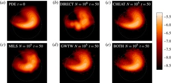
Contour plots of
 $c(\boldsymbol{x},T)R(\boldsymbol{x})$
from the exact (PDE) solution, together with kernel density reconstructions
 $\bar{c}(\boldsymbol{x},T)R(\boldsymbol{x})$
from the Milstein method (MILS) with
 $N=10^{5}$
,
 $N^{\ast }=10^{5}$
and
 ${\it\epsilon}=1\times 10^{-5}$
, are shown in figure 8 (optimal kernel sizes are used). The results are clearly superior to the direct calculation with
 $N=10^{6}$
, for which only around 20 trajectories arrive in
 $\mathscr{R}$
. Figure 7(b) shows
 $\text{MISE}(T)$
for the same set of simulations as in figure 7(a), confirming that performance improves with increasing
 $N^{\ast }$
and that
 ${\it\epsilon}=10^{-4}{-}10^{-5}$
.
(a) Weighted PDE (Eulerian) solution
 $\log _{10}c(\boldsymbol{x},T)R(\boldsymbol{x})$
in the vicinity of the receptor region
 $\mathscr{R}$
. (b–f) Kernel density estimates of
 $\log _{10}c(\boldsymbol{x},T)R(\boldsymbol{x})$
from the stochastic Lagrangian integrations: DIRECT with
 $N=10^{6}$
; CHEAT with
 $N=10^{5}$
; Milstein with
 $N=10^{5}$
(
 $N^{\ast }=10^{5}$
,
 ${\it\epsilon}=10^{-5}$
); GWTW with
 $N=10^{5}$
(
 $N^{\ast }=10^{5}$
,
 ${\it\epsilon}=10^{-5}$
); and finally an experiment combining both methods, also with
 $N=10^{5}$
.

A further disadvantage of the implementation (a)–(d) of Milstein’s method is the expense of calculating and storing the gridded correcting velocity
 $\bar{\boldsymbol{v}}^{\ast }$
, as well as interpolating it during the forward calculations. As is clear from figure 4(b),
 $\bar{\boldsymbol{v}}^{\ast }$
must be obtained and stored at a relatively high temporal resolution (here
 ${\rm\Delta}t=0.1$
). The overall cost of this increases the expense of our forward calculations by around a factor of 10 compared to the direct calculations, significantly reducing the gains made by variance reduction. Fortunately, better results are obtained with the GWTW algorithm, as will be seen next.
4.2. Estimators based on GWTW
To create a purely Lagrangian estimator based on GWTW, steps (a) and (b) are followed as above, followed by:
(c 2) A forward run with GWTW scored according to
 $$\begin{eqnarray}S_{t}={\it\Theta}_{t}(\bar{c}^{\ast }(\boldsymbol{X}_{t},t)+{\it\epsilon}).\end{eqnarray}$$
In close analogy with Milstein’s method, introducing an
 ${\it\epsilon}>0$
acts effectively to switch off GWTW in regions where
 $\bar{c}^{\ast }\ll {\it\epsilon}$
, in order that particles are not removed and added erroneously in regions where the estimate
 $\bar{c}^{\ast }$
of
 $c^{\ast }$
is inaccurate.
The importance of choosing
 ${\it\epsilon}$
to be sufficiently large is seen in the lower two rows of figure 6, which show the trajectory positions in GWTW runs with
 $N^{\ast }=10^{5}$
and
 ${\it\epsilon}=10^{-5}$
(e, f) and
 ${\it\epsilon}=10^{-7}$
(g,h). For the
 ${\it\epsilon}=10^{-7}$
GWTW run, from the
 $t=20$
panel it is clear that some
 $\mathscr{S}\rightarrow \mathscr{R}$
transport pathways are significantly under-resolved, mainly in regions where
 $c(\boldsymbol{x},t)$
is large (e.g. regions highlighted by arrows). The under-resolution is due to trajectories being removed too rapidly from regions where
 $c^{\ast }$
is low, because in these regions there are no back trajectories, meaning that
 $\bar{c}^{\ast }$
is effectively zero and trajectory scores are too low. Elsewhere, there is evidence of erroneous trajectory clustering on the scale of the kernel size
 $h$
, which is due to trajectories being reproduced close to local maxima in
 $\bar{c}^{\ast }$
associated with individual back trajectories. The consequence of the poor sampling of
 $\mathscr{S}\rightarrow \mathscr{R}$
transport pathways in the
 ${\it\epsilon}=10^{-7}$
simulation is that, despite the spatial distribution of particles at
 $t=50$
appearing to be reasonable, there is increased variance in statistics of the trajectory weights at
 $t=50$
, consistent with a relatively poor estimate of
 $\mathscr{I}$
. Choosing
 ${\it\epsilon}=10^{-5}$
improves the sampling of
 $\mathscr{S}\rightarrow \mathscr{R}$
pathways, but at the expense of over-resolving where
 $c$
is large, and consequently a lower proportion of trajectories reaching
 $\mathscr{R}$
at
 $t=50$
. As with Milstein’s method, there is evidently a trade-off between competing effects, and an optimal value of
 ${\it\epsilon}$
for the algorithm.
The performance of GWTW is quantified as a function of
 ${\it\epsilon}$
and
 $N^{\ast }$
in figure 7(c,d). It is clear that our implementation of GWTW performs substantially better than Milstein’s method, with robust behaviour over a wide range of
 ${\it\epsilon}$
centred on the optimal value of around
 $10^{-5}$
. For runs with
 $N^{\ast }=10^{5}$
, the variance is reduced by 2.5 orders of magnitude, increasing to three orders of magnitude for
 $N^{\ast }=10^{6}$
. An even greater improvement over Milstein’s method is evident for
 $\text{MISE}(T)$
, which is also apparent in the kernel density reconstructions of figure 8.
GWTW is also much cheaper to implement than Milstein’s method. Interpolation of
 $\bar{c}^{\ast }$
and sorting of winners and losers happens only at longer intervals
 ${\rm\Delta}t=0.1$
, whereas
 $\bar{v}^{\ast }$
in Milstein’s method must be obtained by interpolation at every SDE time step
 ${\it\delta}t=0.01$
in order to integrate the trajectory weight equation. As a result, GWTW adds only 10 %–20 % to the cost of a forward run, making it remarkably cheap as well as robust. For our model problem, the computational cost of integrating
 $N=10^{5}$
trajectories is comparable to that of using the kernel density method to make 500 constructions of
 $\bar{c}^{\ast }$
from the results, hence the overall cost of the algorithm (backwards run, construction of
 $\bar{c}^{\ast }$
, forwards run) is around three times that of the direct method. In our model problem, fixing a level of accuracy required for
 $\mathscr{I}$
in advance, the GWTW algorithm can obtain the required estimate at roughly 1 % of the computational cost of using the direct method.
5. Conclusions
The focus of this work has been to address the following question: How is transport in an advection–diffusion problem, between a pre-selected source region
 $\mathscr{S}$
and receptor region
 $\mathscr{R}$
, modelled most efficiently using stochastic Lagrangian methods? The main theoretical result, which underpins each of the methods subsequently formulated, and which we believe to be fundamental to the understanding of advection–diffusion problems, is that the ideal distribution of particles is proportional to the density of trajectories field
 $D(\boldsymbol{x},t)$
defined by (2.11). The field
 $D$
is the product of
 $c$
, the solution of the forward transport problem (
 $\mathscr{S}\rightarrow \mathscr{R}$
), and the adjoint solution
 $c^{\ast }$
(
 $\mathscr{R}\rightarrow \mathscr{S}$
). The corresponding ideal particle weights are inversely proportional to
 $c^{\ast }$
.
Motivated by the above observations, a robust and flexible Lagrangian adaptive algorithm has been developed based on the GWTW strategy (Grassberger Reference Grassberger2002). The algorithm uses both forward and back trajectories, with the selection of winners and losers in the forward calculation controlled by an estimate of the adjoint solution, which is obtained from the preliminary backward calculation. In our model problem, trajectories in the adaptive calculation have variance three orders of magnitude lower than those of the direct calculation, with the computational cost increased by just over a factor of two. There is also plenty of room for further optimisation, perhaps most promisingly because the method can be combined with the complementary forward–backward representation of Milstein et al. (Reference Milstein, Schoenmakers and Spokoiny2004).
The GWTW algorithm is particularly suited to advection–diffusion in the chaotic advection regime, in which the underlying deterministic trajectories separate exponentially. Alternative ‘small-noise’ approaches based on large-deviation theory (e.g. Vanden-Eijnden & Weare Reference Vanden-Eijnden and Weare2012) appear to be prohibitively expensive and complicated to implement in chaotic advection. In the method of Vanden-Eijnden & Weare (Reference Vanden-Eijnden and Weare2012), a variational problem is solved for each trajectory, at regular time intervals, to obtain a correcting velocity
 $\boldsymbol{v}$
for use with Milstein’s method. In the chaotic advection regime, the solutions to this variational problem are discontinuous in time and space across multiple interfaces, which are not a priori predictable. This means that a solution for a particular trajectory cannot be found reliably using an iteration that begins with a previous solution.
The main weakness of the GWTW method described here is that it is limited by the measurement ratio
 $\mathscr{I}/S_{00}$
, i.e. the total tracer in the measurement region divided by the total released. Unlike the small-noise methods discussed above, the GWTW method will fail when the measurement ratio is sufficiently low that there is little or no spatial overlap between forward and backward trajectories at intermediate times in the calculation. The Péclet number (
 $\mathit{Pe}$
) dependence of the GWTW method is felt primarily through its influence on this measurement ratio. Further experiments with the simple model here indicate that GWTW will succeed over a wide range of
 $\mathit{Pe}$
provided that the measurement region is chosen so that
 $\mathscr{I}/S_{00}$
is not too small (i.e.
 $\mathscr{I}/S_{00}\gtrsim 10^{-6}{-}10^{-7}$
for the number of trajectories
 $N=10^{5}{-}10^{6}$
used here). However, note that, considering a sequence of flows with increasing
 $\mathit{Pe}$
, the measurement region
 $\mathscr{R}$
will be required to be located increasingly close to the deterministic trajectories to maintain the measurement ratio. Although measurement ratios much smaller than the value (
 ${\approx}2\times 10^{-5}$
) considered here are unlikely to be of much practical interest in fluid problems, it is notable that values of
 $\mathscr{I}/S_{00}$
in the range
 $10^{-10}{-}10^{-20}$
are typical in the molecular dynamics problems that have motivated the development of the small-noise methods. For these problems, which are generally not in the chaotic regime, the small-noise methods discussed above can be used.
Will the GWTW algorithm be straightforward to implement in state-of-the-art operational atmospheric Lagrangian trajectory models, such as FLEXPART (Stohl et al. Reference Stohl, Forster, Frank, Seibert and Wotawa2005) or NAME (Jones et al. Reference Jones, Thomson, Hort, Devenish, Borrego and Norman2007)? Some practical and technical issues must be overcome, such as the increase from two to three dimensions, and the fact that diffusivities in the atmosphere are highly anisotropic, with dispersion in the horizontal primarily driven by a combination of vertical diffusivity and vertical shear in the mean wind (cf. shear dispersion; Taylor Reference Taylor1953). Further, turbulent diffusivities are spatially inhomogeneous, most notably at the top of the atmospheric boundary layer, where there is a rapid decrease. Finally, Poisson (jump) processes are likely to be required in regions of convection (Forster, Stohl & Seibert Reference Forster, Stohl and Seibert2007). Notwithstanding these potential difficulties, in principle there is no obstacle to the suitable adaptation of the principles outlined in this work to the operational scenario.
Acknowledgements
Thanks are due to A. Truong for his collaboration on some preliminary integrations. This work was supported by UK NERC grant NE/G016003/1.
Appendix A. Lower bound on the variance of Milstein’s estimator with uniform drift
In § 3.3, the estimator
 ${\it\Pi}={\it\Theta}_{T}R(\boldsymbol{Y}_{T})$
for
 $\mathscr{I}$
, given by (3.9), was discussed for the case with a uniform correcting velocity
 $\boldsymbol{v}=V\boldsymbol{i}$
. Here we obtain the lower bound (3.17) on its variance.
We will work under the assumption that
 $R(\boldsymbol{x})$
is non-negative and bounded above by a constant
 $C$
(
 $C=1$
in our example). The fact that
 ${\it\Theta}_{0}=S_{00}$
(because
 $g(\boldsymbol{x})=1$
) can then be used to write the inequality
 $$\begin{eqnarray}\mathbb{P}(x<{\it\Pi}<\infty )\leqslant \mathbb{P}(x/CS_{00}<{\it\Theta}_{T}/{\it\Theta}_{0}<\infty ).\end{eqnarray}$$
If the (unknown) probability density of
 ${\it\Pi}$
is introduced as
 ${\rm\pi}(x)$
, (A 1) can be expressed as
 $$\begin{eqnarray}P_{{\rm\pi}}(x)\leqslant P(x/CS_{00}),\end{eqnarray}$$
where the cumulative densities
 $P_{{\rm\pi}}$
and
 $P$
are defined to be
 $$\begin{eqnarray}P_{{\rm\pi}}(x)=\int _{x}^{\infty }{\rm\pi}(q)\text{d}q,\quad P(x)=\int _{x}^{\infty }{\it\rho}(q)\text{d}q,\end{eqnarray}$$
and
 ${\it\rho}(x)$
is the density of the random variable
 ${\it\Theta}_{T}/{\it\Theta}_{0}$
given by (3.16).
Next, note that the variance of
 ${\it\Pi}$
can be written, using integration by parts, as
 $$\begin{eqnarray}\text{Var}({\it\Pi})=\int _{0}^{\infty }x^{2}{\rm\pi}(x)\,\text{d}x-\mathscr{I}^{2}=2\int _{0}^{\infty }T(x)\,\text{d}x-\mathscr{I}^{2},\quad \text{with}~T(x)=\int _{x}^{\infty }P_{{\rm\pi}}(q)\,\text{d}q,\end{eqnarray}$$
where the fact that
 $\mathbb{E}({\it\Pi})=\mathscr{I}$
has been used. Using the inequality (A 2) we can write
 $$\begin{eqnarray}T(x)=\mathscr{I}-\int _{0}^{x}P_{{\rm\pi}}(q)\,\text{d}q\geqslant \mathscr{I}-S_{00}C\int _{0}^{x/S_{00}C}P(q)\,\text{d}q.\end{eqnarray}$$
Next define
 $X=X(t_{\ast },\mathscr{R})$
, where
 $\mathscr{R}=\mathscr{I}/S_{00}C$
satisfies
 $0<\mathscr{R}<1$
, to be the root of the equation
 $$\begin{eqnarray}\int _{0}^{X}P(q)\,\text{d}q=\frac{\mathscr{R}}{2}.\end{eqnarray}$$
After integrating, a nonlinear equation satisfied by
 $X$
is found,
 $$\begin{eqnarray}\text{erfc}\left(\frac{t_{\ast }-4\log X}{4\sqrt{t_{\ast }}}\right)+X\,\text{erfc}\left(\frac{t_{\ast }+4\log X}{4\sqrt{t_{\ast }}}\right)=\mathscr{R},\end{eqnarray}$$
where
 $\text{erfc}(\cdot )$
denotes the complementary error function. The quantity
 $X$
has been defined in order that the inequality
 $$\begin{eqnarray}T(x)\geqslant \mathscr{I}/2,\quad \text{for}~0\leqslant x\leqslant S_{00}CX,\end{eqnarray}$$
is satisfied. As a consequence, because
 $T(x)$
is non-negative everywhere,
 $$\begin{eqnarray}\text{Var}({\it\Pi})=2\int _{0}^{\infty }T(x)\,\text{d}x-\mathscr{I}^{2}\geqslant 2\int _{0}^{XS_{00}C}T(x)\,\text{d}x-\mathscr{I}^{2}\geqslant \mathscr{I}^{2}(X/\mathscr{R}-1)\end{eqnarray}$$
which is (3.17) as required.
For the bound (3.17) to be useful, it is necessary to understand the behaviour of
 $X(t_{\ast },\mathscr{R})$
as
 $t_{\ast }\rightarrow \infty$
for fixed
 $\mathscr{R}$
. Note that, for
 $t_{\ast }\ll 1$
,
 $X\approx \mathscr{R}/2$
and the bound is negative (i.e. useless). At large
 $t_{\ast }$
, the asymptotic behaviour of (A 7) can be seen to be
 $X\sim \exp (t_{\ast }/4)$
, hence the bound will always become useful as
 $t_{\ast }$
(or
 $V$
) increases. For the results discussed in § 3.3, numerical solutions of (A 7) have been obtained using a standard root-finding method.
Appendix B. The zero-variance property of the ‘ideal’ estimator
The result that setting
 $\boldsymbol{v}=\boldsymbol{v}^{\ast }$
in Milstein’s method leads to a zero-variance estimator is a standard one in stochastic calculus (see e.g. exercise 16.2.1 of Kloeden & Platen Reference Kloeden and Platen1992) but is included here as a useful alternative perspective on the results of § 3.4. To show the result, it suffices to apply the multivariate version of Itô’s lemma, which states that, for a smooth function
 $f(\boldsymbol{z},t)$
and a vector-valued random process
 $\boldsymbol{Z}_{t}$
,
 $$\begin{eqnarray}\text{d}\,f(\boldsymbol{Z}_{t},t)=(\partial _{t}\,f)\,\text{d}t+(\boldsymbol{{\rm\nabla}}_{\boldsymbol{z}}\,f)\boldsymbol{\cdot }\text{d}\boldsymbol{Z}_{t}+{\textstyle \frac{1}{2}}\text{d}\boldsymbol{Z}_{t}\boldsymbol{\cdot }\boldsymbol{{\rm\nabla}}_{\boldsymbol{z}}\boldsymbol{{\rm\nabla}}_{\boldsymbol{z}}\,f\boldsymbol{\cdot }\text{d}\boldsymbol{Z}_{t}.\end{eqnarray}$$
The lemma is applied to the stochastic variable
 ${\it\Theta}_{t}\,c^{\ast }(\boldsymbol{Y}_{t},t)$
, with the identification
 $\boldsymbol{Z}_{t}^{\dagger }=(\boldsymbol{Y}_{t}^{\dagger }{\it\Theta}_{t})$
as in § 3.2. Then,
 $$\begin{eqnarray}\displaystyle \text{d}({\it\Theta}_{t}\,c^{\ast }(\boldsymbol{Y}_{t},t)) & = & \displaystyle {\it\Theta}_{t}(\partial _{t}c^{\ast })\,\text{d}t+c^{\ast }\,\text{d}{\it\Theta}_{t}+{\it\Theta}_{t}\boldsymbol{{\rm\nabla}}c^{\ast }\boldsymbol{\cdot }\text{d}\boldsymbol{Y}_{t}\nonumber\\ \displaystyle & & \displaystyle +\,{\textstyle \frac{1}{2}}{\it\Theta}_{t}(\text{d}\boldsymbol{Y}_{t}\boldsymbol{\cdot }\boldsymbol{{\rm\nabla}}\boldsymbol{{\rm\nabla}}c^{\ast }\boldsymbol{\cdot }\text{d}\boldsymbol{Y}_{t})+\text{d}{\it\Theta}_{t}(\text{d}\boldsymbol{Y}_{t}\boldsymbol{\cdot }\boldsymbol{{\rm\nabla}}c^{\ast }).\end{eqnarray}$$
Next, using (3.7) to substitute for
 $\text{d}\boldsymbol{Y}_{t}$
and
 $\text{d}{\it\Theta}_{t}$
, and discarding terms of
 $o(\text{d}t)$
, after some working it can be seen that
 $$\begin{eqnarray}\displaystyle \text{d}({\it\Theta}_{t}\,c^{\ast }(\boldsymbol{Y}_{t},t)) & = & \displaystyle {\it\Theta}_{t}(\boldsymbol{{\rm\nabla}}c^{\ast }-{\textstyle \frac{1}{2}}c^{\ast }\boldsymbol{v}\boldsymbol{\cdot }{\bf\kappa}^{-1})\boldsymbol{\cdot }(2{\bf\kappa})^{1/2}\boldsymbol{\cdot }\text{d}\boldsymbol{W}_{t}-{\it\Theta}_{t}\,\mathscr{L}^{\dagger }c^{\ast }\,\text{d}t\end{eqnarray}$$
 $$\begin{eqnarray}\displaystyle & = & \displaystyle 0\quad \text{on setting}~\boldsymbol{v}=\boldsymbol{v}^{\ast }.\end{eqnarray}$$
 ${\it\Theta}_{T}\,c^{\ast }(\boldsymbol{Y}_{T},T)={\it\Theta}_{0}\,c^{\ast }(\boldsymbol{Y}_{0},0)=\text{const.}$
provided we make the choice
 ${\it\Theta}_{0}=G_{00}c^{\ast }(Y_{0},0)^{-1}$
, or equivalently that
 $g(\boldsymbol{x})=c^{\ast }(\boldsymbol{x},0)$
as anticipated in § 3.4. Since
 ${\it\Theta}_{T}\,c^{\ast }(\boldsymbol{Y}_{T},T)={\it\Theta}_{T}R(\boldsymbol{Y}_{T})$
, we have the desired result that the latter is a deterministic (i.e. zero-variance) estimator of
 $\mathscr{I}$
.