





1. Introduction
Fluids flow through the interconnected networks of pores permeating many engineering, biological and Earth materials. Many of these materials are prone to deformation, so that their pore networks are constantly evolving. Meanwhile, interstitial flow can build or drain pressure in this evolving pore network, modifying the material’s tendency to continue deforming. This feedback loop plays a critical role in the transport of nutrients in bone (Fritton & Weinbaum Reference Fritton and Weinbaum2009; Cardoso et al. Reference Cardoso, Fritton, Gailani, Benalla and Cowin2013) as well as the evolution of the earth materials at our feet (Biot Reference Biot1941; Coussy Reference Coussy2003). One setting in which flow through a permeable, deformable subsurface has global consequences is beneath the massive, grounded glaciers seen across Antarctica and Greenland. Glacial beds are permeated by complex hydrological systems (Walder Reference Walder1982; Murray & Clarke Reference Murray and Clarke1995; Legleiter et al. Reference Legleiter, Tedesco, Smith, Behar and Overstreet2014; Flowers Reference Flowers2015) that can reduce the dissipating stress of the bed (Terzaghi et al. Reference Terzaghi, Peck and Mesri1996; Truffer et al. Reference Truffer, Harrison and Echelmeyer2000; Kjær et al. Reference Kjær, Larsen, van der Meer, Ingólfsson, Krüger, Örn Benediktsson, Knudsen and Schomacker2006; Truffer & Harrison Reference Truffer and Harrison2006) and increase glacier speed (Tulaczyk et al. Reference Tulaczyk, Kamb and Engelhardt2000; Flowers Reference Flowers2015).
Unlike other Earth materials that support static structures, glacial beds underlie dynamic ice masses capable of moving several kilometres per year (Rignot et al. Reference Rignot, Mouginot and Scheuchl2011). In addition to supporting the weight of the glacier, the glacial bed dissipates longitudinal and gravitational driving stresses, and therefore plays a key role in the force balance of glaciers. The hydrological system permeating the glacial bed reduces the dissipating stress of the bed on the glacier through the build-up of fluid pressure (Terzaghi et al. Reference Terzaghi, Peck and Mesri1996; Truffer et al. Reference Truffer, Harrison and Echelmeyer2000; Kjær et al. Reference Kjær, Larsen, van der Meer, Ingólfsson, Krüger, Örn Benediktsson, Knudsen and Schomacker2006; Truffer & Harrison Reference Truffer and Harrison2006;). The extent to which fluid pressure can build up depends on the permeability of the bed.
In some locations, the water-saturated glacial bed consists of deformable porous sediments (Iverson et al. Reference Iverson, Hooyer and Baker1998; Tulaczyk et al. Reference Tulaczyk, Kamb and Engelhardt2000) called subglacial tills (Haldorsen Reference Haldorsen1981). The large weights of glaciers impose massive overburdens and intense shear stresses on subglacial tills (Iverson et al. Reference Iverson, Hooyer and Baker1998; Tulaczyk et al. Reference Tulaczyk, Kamb and Engelhardt2000). Massive overburdens mean that subglacial tills experience significant consolidation compared with other sediments, while intense shear stresses mean that subglacial tills experience significant deformation compared with sedimentary rocks. As a consequence, subglacial tills and their corresponding pore structures are constantly evolving. The presence of a hydrological system that permeates subglacial tills modifies and amplifies this evolution (Tulaczyk et al. Reference Tulaczyk, Kamb and Engelhardt2000; Flowers Reference Flowers2015).
While the pore geometry is constantly evolving, the grain-size distribution of subglacial till remains essentially invariant under deformation, at least on time scales that are short compared with grain-crushing processes. Once the till has experienced significant strain over time, the individual grains of clay (
 ${\sim} 10^{-6}$
m) and sand (
 ${\sim} 10^{-3}$
m) that constitute most tills (e.g. Haldorsen Reference Haldorsen1981; Daigle & Reece Reference Daigle and Reece2014) tend towards a steady-state distribution (Earle Reference Earle2019). Grain-size distributions play a major role in a material’s dominating length scales; a material’s dominating length scales play a major role in the connectivity of its pore geometry (Dagan Reference Dagan1989); and pore geometry plays a major role in a material’s permeability (Bear Reference Bear1972). Better quantifying the relationship between grain-size distribution and permeability could maximise the value of data by using a model rooted in intrinsic material properties, which is especially important in locations where samples are difficult to collect as in the case of glacial beds.
The permeability of subglacial tills is often parametrised through median grain size and porosity (e.g. Damsgaard et al. Reference Damsgaard, Egholm, Piotrowski, Tulaczyk, Larsen and Brædstrup2015), but a material’s porosity only captures the total volume of its pores, not the connectivity of its pore geometry. Porosity can be a robust predictor of permeability when a material consists of roughly homogeneous spheroid grains of minimal size and shape variability (Carman Reference Carman1997). We refer to these materials as idealised because the variability in pore geometry is limited: pore-throat sizes are determined by the median grain size and pore-throat shapes by the sphericity of the grains (Carman Reference Carman1997). The Kozeny–Carman relation closes the relationship between permeability and porosity for idealised materials (Carman Reference Carman1997), but many Earth materials have a very non-uniform pore geometry with very few dominant paths (Berg & van Wunnik Reference Berg and van Wunnik2017). For subglacial tills, such non-uniform geometries arise through multi-modal grain-size distributions, with each mode having its own wide variance.
The goal of this paper is to estimate the permeability of approximately bi-disperse Earth materials from their bulk porosities and grain-size distributions by linking direct numerical simulation with sequential homogenisation. Direct numerical simulations enable us to compute flow fields through any grain-size distribution, although at high computational cost. Sequential homogenisation lowers computational costs by computing flow fields for each grain-size mode separately assuming that the grain-size modes are scale-separated. We validate our model against our laboratory measurements performed on different volume ratios of idealised glass beads and idealised sands. We then test our model against our laboratory measurements performed on samples of approximately bi-disperse subglacial tills from The Polar Rock Repository (PRR) et al. (2015). A summarising schematic outlining the context of the subglacial environments and our methods is presented in figure 1.
Subglacial tills form a soft foundation beneath glaciers, and can be permeated with porewater. The bottom left inset depicts the nature of our laboratory measurements using a compaction permeameter. The top right inset describes the type of pore structures that we study.

Because several orders of magnitude can separate the clay and sand modes of subglacial tills, the grid resolution required to resolve both scales simultaneously using direct numerical simulations is prohibitively expensive. To alleviate computational costs, we separate our subglacial tills into a dual-porosity system (Coussy Reference Coussy2003) composed of pores at the sand length scale and pores at the clay length scale. We use homogenisation to decompose this multi-scale system into a coupled set of systems for each scale assuming length-scale separation (Hornung Reference Hornung1997). Since homogenisation allows us to simulate each scale separately, our grids no longer need to resolve multiple scales. We build upon the sequential homogenisation procedure of Mei & Auriault (Reference Mei and Auriault1989) to compute bulk permeability when the small pores at the clay length scale fill the large pores of the sand length scale. We also incorporate a homogenisation step similar to that used by Sáez et al. (Reference Sáez, Otero and Rusinek1989) to estimate the bulk permeability of a heterogeneous unit cell that has part of its geometry at one permeability and the remainder of the geometry at another permeability.
Homogenisation is useful for decomposing our subglacial till domain into its scale-separated modes, but it does not help with representing the wide variances and unique distribution seen in each of the subglacial till’s modes. Instead of using an analytical approach to complete the homogenisation procedure, we use a discrete element method (DEM) to generate samples of physical granular packings adhering to a particle grain-size distribution, following the work of Schenker et al. (Reference Schenker, Filser, Herrmann and Gauckler2009) and Kloss et al. (Reference Kloss, Goniva, Hager, Amberger and Pirker2012). We then perform our own direct numerical simulations of flow through these granular packing samples assuming a fixed solid skeleton, since Kasmalkar et al. (Reference Kasmalkar, Damsgaard, Goren and Suckale2021) showed that shear-induced deformation of the solid skeleton occurs at a different time scale than fluid flow in subglacial tills.
We show that our model enables us to analyse the interaction between a medium’s grain-size distribution and the complex flow geometry through its pores. While our primary motivation is to estimate the permeability of subglacial tills, our approach applies to other bi-disperse materials with two scale-separated modes of grain sizes.
2. Laboratory measurements
2.1. Grain-size distributions and sediment samples
In the laboratory, we collect data on grain-size distribution, porosity and hydraulic conductivity for both idealised and Earth materials: For our idealised materials, we create mixtures of glass shot and sand that we then compare them with natural subglacial tills.
To have a benchmark for our modelling, we aim to produce bi-modal distributions of two discrete grain sizes separated by approximately one order of magnitude. The actual separation we obtain is limited by the resolution of the mesh sizes bracketing each retained sample. We use spheroidal glass shot passed through a 180
 ${\unicode[Arial]{x03BC}}$
m mesh (No. 80 sieve) that was retained on a 150
 ${\unicode[Arial]{x03BC}}$
m mesh (No. 100 sieve). We mix this material with well-rounded quartz beach sand, sourced from the Bayfield Peninsula, Wisconsin, passed through a 2 mm mesh (No. 10 sieve) and retained on a 1 mm mesh (No. 18 sieve). Ultimately, we produce two approximately normal populations with mean diameters centred at 160
 ${\unicode[Arial]{x03BC}}$
m
 $(\sigma _{F} = 29.7$
 ${\unicode[Arial]{x03BC}}$
m
 $)$
and 1500
 ${\unicode[Arial]{x03BC}}$
m
 $(\sigma _{C} = 320$
 ${\unicode[Arial]{x03BC}}$
m
 $)$
for the shot and sand, respectively. We then mix these two contrasting materials together in three different proportions of volume – approximately 1 : 10, 1 : 1 and 10 : 1 shot to sand.
We measure the grain diameters for each idealised material using laser diffraction analysis (Malvern Mastersizer 2000E, range 0.01–2000
 ${\unicode[Arial]{x03BC}}$
m). Before analysis, we wash and dry the samples to remove fines and prevent aggregation, then disperse them in deionised water. For each material, we perform three replicate runs, reporting our results as the volume-based median diameter (
 $d_{50}$
). For coarse sand, the particle sizes approach the upper detection limit of the instrument, making laser diffraction unreliable. Instead, we estimate grain diameters through image analysis. We photograph a representative subsample (
 $n \approx 200$
grains) on a lightboard under uniform illumination, with scale calibration provided by a stage micrometer. We then process the images using ImageJ software to calculate equivalent circular diameters, accounting for the irregularity of grain shapes.
Image of our mixture of two idealised synthetic materials alongside component grain-size distributions (top row) and image of subglacial till alongside grain-size distribution (bottom row). (a) Image of our mixture of glass shot and sand grains. (b) Grain-size distribution for fine glass shot. (c) Grain-size distribution for coarse sand grains (bottom). Relative frequencies are represented as bars, with best fit normal distributions as opaque dotted lines. (d) Image of subglacial till sampled from a deglaciated paleo deposit of the Bindschadler Ice Stream in West Antarctica. (e) Corresponding grain-size distribution for Bindschadler subglacial till.

Figure 2. Long description
Panels a-c show an idealized mixture, a close-up of fine glass beads, and histograms with normal fits for fine beads near 162 micrometers and coarse sand near 1,460 micrometers. Panels d-e show an image of Bindschadler Till and its broad, bimodal grain-size distribution. The inset enlarges the fine mode on a logarithmic grain-size axis.
We also conduct hydraulic conductivity experiments on a suite of natural tills from Antarctica. Ten of these tills were collected in the field and are now archived at The Polar Rock Repository (PRR) et al. (2015), along with one subglacial till sampled from a paleo–grounding zone of the Bindschadler Ice Stream (McGlannan et al. Reference McGlannan, Bart, Chow and DeCesare2017). The PRR samples represent a range of terrains and lithologies with further details for each sample available in the PRR database under the corresponding sample names. Although the precise genesis and depositional history of each sample are uncertain, they share key characteristics of basal tills, most notably a wide variance in grain sizes. For analysis, we remove clasts larger than 2 mm and then measure grain-size distributions of the processed sediments by laser diffraction using a Malvern Mastersizer, following standard protocols.
In figure 2, we compare the idealised mixture with the real Earth material both in appearance and in grain-size distribution. An example mixture of idealised materials is shown in figure 2(a), with an inset highlighting the fine glass shot. Histograms of grain sizes for the fine glass shot and coarse sand are shown in figures 2(b) and 2(c), respectively, along with fitted normal distributions obtained using maximum likelihood estimation. The fine glass shot histogram is coloured light blue, distinguished from the coarse sand histogram coloured in black. Both histograms and Gaussian fits are tightly centred on their respective modes, with normalised standard deviations (SDs) of
 $\sigma _{F} / \mu _{F} = 0.18$
for the fine mode and
 $\sigma _{C} / \mu _{C} = 0.21$
for the coarse mode. The two modes are separated in scale by roughly one order of magnitude, with
 $\mu _{F} / \mu _{C} = 0.11$
.
We show an example scanning electron microscopy (SEM) image of the subglacial till from Bindschadler Ice Stream (McGlannan et al. Reference McGlannan, Bart, Chow and DeCesare2017) in figure 2(d). The large image highlights some of the coarse sand grains and the inset highlights the extremely small and heterogeneous clay grains. We plot the corresponding probability distribution function of the grain sizes in figure 2(e), with an inset that represents the magnitude of the fine clay mode. Like the distinct colours used in figures 2(b) and 2(c), light blue is used in the inset of figure 2(e) to distinguish the fine mode from the coarse mode. The magnitudes and widths of the fine mode and coarse mode differ greatly for the till, making it challenging to assess the relative amount of fine grains and coarse grains visually. By directly computing the areas under the curve for the blue region and white regions, we find that the fraction of fine grains (
 $0.68$
) is of comparable magnitude to the fraction of coarse grains (
 $0.32$
).
When comparing the grain-size distributions in figures 2(b,c) and 2(e), the two modes of the idealised mixture are very different from the two modes of the subglacial till. In the idealised mixture, both the fine and coarse modes exhibit little variance relative to their mean grain size, the modes are separated by roughly an order of magnitude and the distributions for each mode do not interfere with each other at all. However, the subglacial till exhibits less clear separation: the fine and coarse modes see wide variances relative to their mean grain size, the modes are not very separated and the distributions for each mode clearly interfere with each other. In figure 3, we plot grain-size distributions of several PRR tills with an inset for the large peak for the mode at around 0.1–10
 ${\unicode[Arial]{x03BC}}$
m. Subglacial tills have varying degrees of overlap among the two primary modes of grain sizes, and sometimes have additional modes (such as PRR 23842) or only a single distinguishable mode (such as PRR 23943).
2.2. Measuring hydraulic conductivity
We measure hydraulic conductivity in a four-inch diameter Gilson
 $^{\text{TM}}$
rigid-wall compaction-mould permeameter using the constant head method, following ASTM D5856-15 (ASTM International 2015). The only exception is Bindschadler Till, which has high clay content and low conductivity, and could not be tested in the rigid-wall device. Instead, we use a six-inch diameter flexible-wall permeameter with the falling head method, following ASTM D5084, to measure conductivity at three different porosities. For the idealised mixtures and the Bindschadler Till, we measure conductivity at multiple porosities, whereas each PRR till was tested at a single porosity. We achieve variable porosities by compacting samples in the appropriate mould to a target density. We estimate the resultant porosities from water content, mass and density using procedures outlined in the respective ASTM standards. Reported values of hydraulic conductivity from the constant head tests represent the mean of six measurements collected during a single experiment, while flexible-wall permeameter results represent averages of multiple measurements collected over 1–2 weeks of run time.
Because the material samples contain clay, the influence of clay swelling during fluid injection for hydraulic-conductivity measurements cannot be neglected (Scheuerman & Bergersen Reference Scheuerman and Bergersen1990). Tap water was used as the probing fluid, which should have reduced the likelihood of swelling relative to very low ionic-strength water. However, the ionic composition was not independently measured or controlled. Because several samples contain appreciable montmorillonite, fluid–clay interactions may still have influenced the measured hydraulic conductivities by altering pore-structure during measurement. Accordingly, the reported values are interpreted as effective conductivities under the experimental conditions employed, rather than intrinsic values independent of pore-fluid chemistry.
Grain-size distribution for several subglacial tills. Insets depict the fine mode at approximately 0.1–10
 ${\unicode[Arial]{x03BC}}$
m.

We report corresponding permeabilities because permeability removes the direct dependence of hydraulic conductivity on fluid density and viscosity, although it does not remove changes to the medium caused by fluid–solid interactions. Because our laboratory measurements are conducted using a constant head method with water at room temperature, we compute an effective permeability
 $k$
from the measured hydraulic conductivity
 $K$
using the relation:
 \begin{align} k = \frac {\mu }{\rho g}K , \end{align}
where we use
 $\mu = 1.0\times 10^{-3}$
Pa s as the dynamic viscosity of water at
 $20\,^\circ\textrm{C}$
,
 $g = 9.8$
m s
 $^{-2}$
as the acceleration due to gravity and
 $\rho = 1.0 \times 10^3$
kg m
 $^{-3}$
as the density of water at
 $20\,^\circ\textrm{C}$
(Kestin et al. Reference Kestin, Sokolov and Wakeham1978). We list these measured hydraulic conductivities and effective permeabilities for the subglacial tills from The Polar Rock Repository (PRR) et al. (2015) in table 1. While these subglacial tills have low permeabilities relative to other granular materials, tills have high permeabilities relative to many rocks that have been the object of many observations (Mahesar et al. Reference Mahesar, Memon, Memon and Tunio2017; Scott et al. Reference Scott, Lévy, Covell, Franzson, Gibert, Valfells, Newson, Frolova, Júlíusson and Guđjónsdóttir2023; Vali & Haji Zadeh Reference Vali and Haji Zadeh2024). In particular, these tills have permeabilities above the 1 mD, or
 $9.8 \times 10^{-16}$
m
 $^2$
, limit where the choice of interstitial fluid used for measurement can lead to differences of orders of magnitude (Mahesar et al. Reference Mahesar, Memon, Memon and Tunio2017).
Summary of laboratory measurements including grain-size distributions, as well as hydraulic conductivities and corresponding bulk permeabilities. Grain size data for idealised materials as well as more complete data for different tills from the Polar Rock Repository.

3. Model
We derive a model to estimate permeability from grain-size distribution using steady fluid mechanics through geometries and test our estimates against laboratory measurements from the samples described in § 2. Our model consists of four components.
-
(i) Conceptualisation of the Dual Porosity Space (§ 3.1) describes our model domain and how we constrain it using the data available from laboratory measurements.
-
(ii) Sequential Homogenisation for Upscaling (§ 3.2) derives a set of partial differential equations using a homogenisation procedure to upscale from the fine-scale to the system-scale.
-
(iii) Numerical Homogenisation Procedure (§ 3.3.1) discusses how we implement the partial differential equations of § 3.2 for geometries generated through the methods of § 3.4.
-
(iv) Generation of Equivalent Pore Geometries (§ 3.4) describes how we generate pore geometries based on the conceptualisation of the dual porosity space.
3.1. Conceptualising the dual porosity space
Some properties of granular materials, such as grain-size distribution, can be measured directly. Other properties, such as porosity, represent material averages and can only be measured in bulk. Bulk porosities capture the total amount of open space for water to travel through in a sample of material, but do not reveal how the open space is spatially distributed. At one extreme, a material with a given porosity could have a small number of large pores on a coarse length scale. At the other extreme, a material with the same porosity could have a large number of small pores at a fine length scale.
To address the variability of pore sizes in our model, we simplify the distribution of pore sizes into a dual-porosity system with pores of coarse-scale size and pores of fine-scale size. We then use the two modes of the grain-size distribution to estimate how much of the material likely consists of sparse coarse-scale pores or dense fine-scale pores. Using these data, we reduce some of the rich variability expected in the pore geometry to a deterministic system for our study.
Figure 4 shows our conceptualisation of the multi-scale pore geometry. To understand the dynamics of a polydisperse sediment layer,
 $\varOmega '''$
, with thickness
 $l'''$
, we study a unit cell
 $\varOmega ''$
consisting of three components:
 $\varOmega _{C}$
(khaki) represents the subdomain consisting of only coarse grains;
 $\varOmega _{\textit{CF}}$
(brown with khaki spots) represents the subdomain consisting of fine and coarse grains; and
 $\varOmega _{F}$
(brown) represents the subdomain consisting of only fine grains. Light blues representing porewater fill the spaces between khaki circles representing coarse grains in the coarse domain
 $\varOmega _C$
. The brown spaces representing fine grains fill the spaces between the khaki circles representing coarse grains in the coarse domain
 $\varOmega _C'$
. The domain
 $\varOmega _F$
consists of only fine grains, occupying the spaces between coarse grains in
 $\varOmega _C'$
, as well as having its own part of the domain in the large unit cell
 $\varOmega ''$
. Light blues representing pore water fill the spaces between brown circles representing fine grains in
 $\varOmega _F$
. The wide variance in the size of brown circles corresponds to the wide variance often seen in the size of fine grains. We indicate a length scale for each domain:
 $l'''$
corresponds to the system domain scale,
 $l''$
corresponds to the length scale for compositional fluctuations,
 $l'$
corresponds to the coarse grain size and
 $l$
represents the fine grain size.
Diagram depiction of our conceptualised model domain. The domain
 $\varOmega '''$
with attached thickness
 $l'''$
is the overall system scale for which we are interested in estimating permeability. The inset subdomain
 $\varOmega ''$
consists of three component subdomains:
 $\varOmega _C$
(khaki) with entirely coarse grains,
 $\varOmega _{\textit{CF}}$
(brown with khaki hatches) with fine grains in the pores of coarse grains and
 $\varOmega _F$
(brown) with entirely fine grains. Variations in these subdomains happen at length scale
 $l''$
. Both subdomains
 $\varOmega _C$
and
 $\varOmega _C'$
insets have khaki coarse grains with their sizes
 $l'$
defining the length scale, but
 $\varOmega _C$
is filled with porewater (light blue) and
 $\varOmega _C'$
has fines (brown) within its pores. The subdomain
 $\varOmega _F$
has brown fine grains defining its length scale
 $l$
and the pores of
 $\varOmega _F$
are filled with porewater (light blue). The subdomain
 $\varOmega _F$
has the smallest length scale, indicated with the highest associated powers of
 $\epsilon$
.

The fine-component fraction,
 $c$
, is the volume fraction of the grain-size distribution belonging to the fine mode. For our idealised experiments, we determine
 $c$
as we create the sample. For our bimodal tills, we identify the fine mode from the coarse mode by identifying the grain size
 $d_{s}$
corresponding to the lowest local minimum in the grain-size distribution. The fine-component fraction,
 $c$
, corresponds to the total area of the grain-size distribution below
 $d_{s}$
. Then,
 $\phi _T$
is the bulk porosity of the granular medium and is measured directly in the laboratory. The bulk porosity,
 $\phi _T$
, represents the total volume through which water flows per unit volume of bulk material.
In our notation,
 $\phi _i(\varOmega _{\kern-1pt j})$
represents the porosity of the component
 $i$
in the
 $\varOmega _{\kern-1pt j}$
subdomain. We take
 $\phi _{C}(\varOmega _{C})$
to be the porosity of the coarse grains in
 $\varOmega _{C}$
and
 $\phi _{F}(\varOmega _{F})$
to be the porosity of the fine grains in
 $\varOmega _{F}$
. Since
 $\varOmega _{C}$
only has coarse grains and
 $\varOmega _{F}$
only has fine grains,
 $\phi _{F}(\varOmega _{C})$
and
 $\phi _{C}(\varOmega _{F})$
are not needed. However,
 $\varOmega _{\textit{CF}}$
has both fine and coarse grains that contribute to its bulk porosity, and these porosities may be distinct from their counterparts in other subdomains. We take
 $\phi _{C}(\varOmega _{\textit{CF}})$
to be the porosity of the coarse grains in
 $\varOmega _{\textit{CF}}$
. We take
 $\phi _{F}(\varOmega _{\textit{CF}})$
to be the porosity of the fine grains that fill the pores between the coarse grains in
 $\varOmega _{\textit{CF}}$
.
Within a representative volume element, the portion of the domain
 $\varOmega ''$
composed of
 $\varOmega _{C}$
,
 $\varOmega _{F}$
and
 $\varOmega _{\textit{CF}}$
varies. We take these subdomain fractions to be
 $\varPhi _{C}$
,
 $\varPhi _{F}$
and
 $\varPhi _{\textit{CF}}$
, respectively, so that
 $\varPhi _{C} + \varPhi _{F} + \varPhi _{\textit{CF}} = 1$
.
The total volume of fine grains
 $v_{F,T}$
and the total volume of coarse grains
 $v_{C,T}$
in a unit volume provides two additional constraints. We use the corresponding notation convention for
 $v$
as we used for
 $\phi$
, so that
 $v_i(\varOmega _{\kern-1pt j})$
represents the volume of the component
 $i$
in the
 $\varOmega _{\kern-1pt j}$
subdomain. Contributions to the total volume of coarse grains in a representative volume element come from the
 $\varOmega _C$
subdomain or from the
 $\varOmega _{\textit{CF}}$
subdomain. Contributions to the total volume of fine grains in a representative volume element come from the subdomain
 $\varOmega _F$
or from the pores of the coarse grains in the subdomain
 $\varOmega _{\textit{CF}}$
. Using our notation, this comes out as follows:
 \begin{align} v_{C,T} &= \varPhi _Cv_C(\varOmega _C) + \varPhi _{\textit{CF}}v_C(\varOmega _{\textit{CF}}), \nonumber \\[6pt]v_{F,T} &= \varPhi _F v_F(\varOmega _F) + \varPhi _{\textit{CF}} \phi _C(\varOmega _{\textit{CF}}) v_F(\varOmega _{\textit{CF}}) \, . \end{align}
From our information about the bulk,
 $1-\phi _T$
is the total bulk volume fraction of solids, meaning the total volume fraction of fines is
 $v_{F,T} = c(1-\phi _T)$
and the total volume of coarse grains is
 $v_{C,T} = (1-c)(1-\phi _T)$
. Because for a representative volume element, all
 $v_i(\varOmega _{\kern-1pt j}) = 1 - \phi _i(\varOmega _{\kern-1pt j})$
,
 \begin{align} c(1-\phi _T) &= \varPhi _{F}(1-\phi _{F}(\varOmega _{F})) + \varPhi _{\textit{CF}}\phi _{C}(\varOmega _{\textit{CF}})(1-\phi _{F}(\varOmega _{\textit{CF}})), \nonumber \\[6pt](1-c)(1-\phi _T) &= \varPhi _{\textit{CF}}(1-\phi _{C}(\varOmega _{\textit{CF}})) + \varPhi _{C}(1-\phi _{C}(\varOmega _{C})) \, . \end{align}
We assume that particle sorting does not occur so that a representative volume element can have either a
 $\varOmega _{F}$
subdomain or a
 $\varOmega _{C}$
subdomain, but not both. Mathematically, this corresponds to the constraint
 $\varPhi _{F}\varPhi _{C}=0$
. The assumption is motivated by observations of ring shear experiments (e.g. Hooyer & Iverson Reference Hooyer and Iverson2000) under high normal stress in which shear strain results in mixing of compositions rather than separation.
Our system for six conceptual properties (
 $\varPhi _{C}, \varPhi _{F}, \phi _{F}(\varOmega _{\textit{CF}}), \phi _{C}(\varOmega _{\textit{CF}}), \phi _{F}(\varOmega _{F}), \phi _{C}(\varOmega _{C})$
) still remains underconstrained. For our study, we assume
 $\phi _{F}(\varOmega _{F})$
and
 $\phi _{C}(\varOmega _{C})$
to be material constants, and we assume that
 $\varPhi _C=\varPhi _C(c)$
and
 $\varPhi _F=\varPhi _F(c)$
are linear in the fine-component fraction. During calibration, we lower bound all porosities using the densest close packings of spheres,
 $\phi = 0.26$
. We upper bound all porosities using the gravitational packing corresponding to the material. Once the functions
 $\varPhi _C(c), \varPhi _F(c)$
are calibrated, our system for conceptual properties is fully constrained.
3.2. Sequential homogenisation of Stokes and seepage flow
We solve the momentum equation in the limit of negligible inertia assuming that the pore fluid is incompressible and satisfies no-slip on solid surfaces. This limit corresponds to the following incompressible Stokes problem in index notation:
 \begin{align} \begin{aligned} \partial _i u_i &= 0, \\[4pt]\partial _i p &=\mu \partial _{\kern-1pt j} \partial _{\kern-1pt j} u_i, \\[4pt]u_i &= 0 \quad \textrm{on} \, \varGamma \, , \end{aligned} \end{align}
where
 $\varGamma$
is the boundary of any solid surfaces in the computational domain.
From here, we follow the sequential homogenisation procedure reflective of Mei & Auriault (Reference Mei and Auriault1989), establishing two distinct types of coarse-graining. At the smallest scale where the fluid–solid pore geometry is explicitly resolved, we homogenise the Stokes problem to obtain an effective Darcy permeability. At all larger scales, the pore space has already been represented by an effective permeability, so we perform consecutive homogenisation steps of seepage problems through a heterogeneous Darcy medium to obtain bulk permeabilities applicable at larger scales.
Thus, we solve Stokes cell problems that do not always begin at the same physical scale, beginning when the fine-grain scale is resolved as in
 $\varOmega _F$
, or beginning at coarser grain-scales as in
 $\varOmega _C$
. Once the first Stokes homogenisation has been performed, all subsequent steps use the same seepage homogenisation procedure iteratively. Rather than carrying out a single perturbation expansion over all four length scales of the system problem, we illustrate the two homogenisation steps as a sequence of adjacent-scale problems. At each step,
 $\epsilon$
denotes the ratio between two neighbouring length scales.
3.2.1. Homogenisation of the Stokes problem
Let
 $\varOmega$
be the periodic representative cell at the smallest scale for which the fluid–solid pore geometry is resolved and let
 $\varGamma$
be the solid boundaries of grains. We define
 $\epsilon$
such that
 $l \sim \epsilon l'$
. For coarse-graining through this
 $l$
-scale, we first assume that the characteristic pressure gradient operates at the adjacent scale
 $l'$
, suggesting the following non-dimensionalisation:
 \begin{align} x_i \sim lx_i^* , \quad p \sim Pp^* ,\quad u_i \sim \frac {Pl^2}{\mu l'}u_i^* . \end{align}
After removing the
 $^*$
superscript, our non-dimensional equations are:
 \begin{align} \begin{aligned} \partial _i u_i &= 0, \\ \partial _i p &= \frac {l}{l'}\partial _i \partial _i u_{\kern-1pt j} = \epsilon \partial _{\kern-1pt j} \partial _{\kern-1pt j} u_i, \\ u_i &= 0 \quad \textrm{on} \, \varGamma . \end{aligned} \end{align}
We define a corresponding spatial coordinate such that spatial variations in
 $\boldsymbol{x} := x_i$
are at the finest-scale and
 $\boldsymbol{x'} := x'_i$
are at the adjacent, coarse-grained scale:
 \begin{align} \boldsymbol{x'} := x'_i \sim \frac {l}{l'} x_i =\epsilon x_i . \end{align}
This means that the gradients at the different scales are
 \begin{align} \partial _i' := \frac {\partial }{\partial x'_i} \sim \frac {\partial }{\partial (\epsilon x_i)} = \frac {1}{\epsilon } \partial _i \, . \end{align}
We then conduct a perturbation expansion in the pressure and velocity fields to match the Stokes momentum equation to leading order:
 \begin{align} p &= p^{[0]}+\epsilon p^{[1]}+\textrm{h.o.t.} , \\[-12pt] \nonumber \end{align}
 \begin{align} u_i &= u_i^{[0]}+\epsilon u_i^{[1]}+\textrm{h.o.t.} . \\[10pt] \nonumber \end{align}
For our perturbed Stokes problem, the incompressibility condition
 $\partial _i u_i = 0$
expands to
 \begin{align} ( \partial _i + \epsilon \partial '_i ) & \left(u_i^{[0]} + \epsilon u_i^{[1]} \right) = 0, \\[-12pt] \nonumber \end{align}
 \begin{align} O( \epsilon ^{0} ) &: \partial _i u_i^{[0]} = 0, \\[-12pt] \nonumber \end{align}
 \begin{align} O( \epsilon ^{1}) &: \partial _i u_i^{[1]} + \partial '_i u_i^{[0]} = 0 . \\[10pt] \nonumber \end{align}
The momentum equation
 $\partial _i p = \epsilon ^3 \partial _i \partial _i u_{\kern-1pt j}$
expands to
 \begin{align} \left(\partial _i + \epsilon \partial '_i \right) \big(p^{[0]} + \epsilon p^{[1]} \big) = \epsilon \left( \partial _i + \epsilon \partial '_i \right)^2 \left(u_{\kern-1pt j}^{[0]} + \epsilon u_{\kern-1pt j}^{[1]} \right) , \end{align}
with
 \begin{align} O(\epsilon ^{0}) &: \partial _i p^{[0]} = 0, \\[-12pt] \nonumber \end{align}
 \begin{align} O(\epsilon ^{1}) &: \partial '_i p^{[0]} + \partial _i p^{[1]} = \partial _{\kern-1pt j} \partial _{\kern-1pt j} u_i^{[0]}. \\[10pt] \nonumber \end{align}
The no-slip boundary condition at the grain boundaries applies to all perturbation terms of the velocity
 $u_i^{[0]}\rvert _{\varGamma }= u_i^{[1]}|_{\varGamma } = 0$
. However, the assumption of periodicity on
 $\varOmega$
imposes a periodic boundary condition on
 $u_i^{[0]}, u_i^{[1]}$
and
 $p^{[0]}, p^{[1]}$
on cell boundaries
 $\partial \varOmega \setminus \varGamma$
.
Our (3.14) implies that
 $p^{[0]}$
only varies in
 $\boldsymbol{x'}$
, i.e.
 $p^{[0]}(\boldsymbol{x'})$
. If we view
 $\partial _i$
and
 $\partial _l\partial _l$
in (3.15) as linear operators acting on
 $p^{[1]}$
and
 $u_i^{[0]}$
, it follows that there should exist some solution pair (
 $p^{[1]}$
,
 $u_i^{[0]}$
) that can be expressed directly as a linear transformation of
 $\partial _i' p^{[0]}$
, i.e.
 \begin{align} p^{[1]} &= S_i\partial '_i p^{[0]} , \\[-12pt] \nonumber\end{align}
 \begin{align} u_i^{[0]} &= -k_{\textit{ij}}\partial '_{\kern-1pt j} p^{[0]} , \\[10pt] \nonumber \end{align}
where tensor
 $k_{\textit{ij}}(\boldsymbol{x}, \boldsymbol{x'})$
and vector
 $S_i(\boldsymbol{x}, \boldsymbol{x'})$
are functions of all spatial scales. Inserting (3.16) and (3.17) back into the momentum balance, (3.15), and the incompressibility condition, (3.11), we can establish a set of equations for
 $k_{\textit{ij}}$
and
 $S_i$
:
 \begin{align} \begin{aligned} \partial _i k_{\textit{ij}} &= 0, \\[3pt]\delta _{\textit{ij}} + \partial _i S_{\kern-1pt j} &= \partial _l \partial _l k_{\textit{ij}} ,\\[3pt]k_{\textit{ij}} = 0 &\quad \textrm{on} \, \varGamma, \\[3pt]k_{\textit{ij}}, S_{\kern-1pt j} \quad &\textrm{periodic over} \, \varOmega. \end{aligned} \end{align}
With this solution, we can now perform an averaging procedure over this smallest scale cell
 $\varOmega$
. The averaging operator
 $\left \langle f \right \rangle _{{\varOmega }}$
over
 $\varOmega$
appears as
 \begin{align} \left \langle f \right \rangle _{{\varOmega }}(\boldsymbol{x'}) = \frac {1}{|\varOmega |}\int _\varOmega \text{d}V_{\boldsymbol{x}} f(\boldsymbol{x}, \boldsymbol{x'}) \, , \end{align}
where
 $\left \langle f \right \rangle _{{\varOmega }}$
is only a function of the larger length scales. The upscaling of the velocity
 $u_i^{[0]}$
only requires the upscaling of the tensor
 $k_{\textit{ij}}(\boldsymbol{x}, \boldsymbol{x'})$
into a slowly varying tensor
 $k_{\textit{ij}}' := \left \langle k \right \rangle _{{\varOmega ,\textit{ij}}}( \boldsymbol{x'})$
. This upscaled tensor is the homogenised Darcy permeability for the next consecutive scale and is symmetric positive definite (Mei & Auriault Reference Mei and Auriault1989). Applying the averaging procedure to the incompressibility condition (3.12) demonstrates that the Darcy permeability tensor solves the corresponding Darcy’s law:
 \begin{align} \frac {1}{|\varOmega |}\int _\varOmega \text{d}V_{\boldsymbol{x}} \left(\partial _i u_i^{[1]} + \partial '_i u_i^{[0]} \right) &= 0 , \\[-28pt] \nonumber\end{align}
 \begin{align} \frac {1}{|\varOmega |}\int _{\partial \varOmega } \text{d}S_{\boldsymbol{x}}n_i u_i^{[1]} + \partial '_i \left \langle u_i^{[0]} \right \rangle _{{\varOmega }} &= 0, \\[-28pt] \nonumber\end{align}
 \begin{align} \partial '_i \left \langle u_i^{[0]} \right \rangle _{{\varOmega }} &= 0 , \\[-28pt] \nonumber \end{align}
 \begin{align} -\partial '_i \left (k'_{\textit{ij}}\partial '_{\kern-1pt j}p^{[0]}\right ) &= 0 \, . \\[0pt] \nonumber\end{align}
3.2.2. Homogenisation of the Poisson-like seepage problem
At larger scales, the pore geometry is no longer resolved explicitly. Instead, the medium is described by a spatially variable Darcy permeability tensor
 $k_{\textit{ij}}(\boldsymbol{x},\boldsymbol{x'})$
. Let
 $\varOmega$
now represent the porous domain for the seepage problem and now let
 $\varGamma$
represent the impermeable internal boundaries of
 $\varOmega$
. Starting from Darcy’s law that was the result of the homogenisation of the Stokes problem, we can recover the general equation without imposed length scales:
 \begin{align} \partial _i \left (k_{\textit{ij}} \partial _{\kern-1pt j} p\right ) = 0. \end{align}
The homogenisation of the seepage problem at this scale is formulated as large scale pressure gradients over
 $l' \sim \epsilon ^{-1}l$
are balanced by small scale variability in mass transport through pores at scale
 $l$
. We expand the pressure again over one order in
 $\epsilon$
and use the same convention:
 \begin{align} p &= p^{[0]}+\epsilon p^{[1]}+\textrm{h.o.t.}\, , \end{align}
with
 $p^{[0]}=p^{[0]}(\boldsymbol{x'})$
. Substituting the pressure expansion into (3.24), we find that
 \begin{align} \big(\partial _i + \epsilon \partial '_i \big) \left ( k_{\textit{ij}} \big(\partial _{\kern-1pt j}+\epsilon \partial '_{\kern-1pt j} \big) \big(p^{[0]} + \epsilon p^{[1]} \big) \right )= 0 \, , \end{align}
which, to leading order, has
 \begin{align} O(\epsilon ^1): \partial _i \left ( k_{\textit{ij}}\big(\partial '_{\kern-1pt j} p^{[0]} + \partial _{\kern-1pt j} p^{[1]} \big)\right )= 0 \, . \end{align}
Once again, the
 $\partial$
gradient can be treated as a linear operator similar to the homogenisation of the Stokes problem. As a result, (3.27) can be satisfied by a solution where
 $p^{[1]}$
is related to
 $\partial '_{\kern-1pt j} p^{[0]}$
by a linear transformation, i.e.
 \begin{align} p^{[1]} = S_{\kern-1pt j}\left (\partial '_{\kern-1pt j} p^{[0]}\right ) \, . \end{align}
Substituting this expression for
 $p^{[1]}$
into (3.27),
 \begin{align} \partial _i \left [k_{\textit{ij}} \left ((\delta _{jl} + \partial _{\kern-1pt j} S_l)\partial '_l p^{[0]}\right )\right ] = 0 \, \quad \forall \partial '_l p^{[0]} \, , \end{align}
we obtain the following vector Poisson equation for the value of
 $S_{\kern-1pt j}$
over the domain
 $\varOmega '$
:
 \begin{align} \begin{aligned} \partial _i (k_{\textit{ij}} \delta _{jl}) &= -\partial _i (k_{\textit{ij}} \partial _{\kern-1pt j} S_l), \\[4pt]n_i k_{\textit{ij}}\left (\delta _{jl}+\partial _{\kern-1pt j} S_l\right )&=0 \quad \textrm{on} \, \varGamma, \\[4pt]S_l \quad &\textrm{periodic over} \, \varOmega , \end{aligned} \end{align}
with a zero normal flux boundary condition corresponding to that used for seepage flow.
With this solution, we can now perform our averaging procedure on the seepage Darcy flux within (3.27) over the seepage
 $\varOmega$
,
 \begin{align} q_i^{[0]} &= \left \langle k_{\textit{ij}}\left(\partial '_{\kern-1pt j} p^{[0]} + \partial _{\kern-1pt j} p^{[1]} \right) \right \rangle _{{\varOmega }} \\[-12pt] \nonumber \end{align}
 \begin{align} &= \left \langle k_{\textit{ij}}(\delta _{jl} + \partial _{\kern-1pt j} S_l)\left(\partial '_l p^{[0]} \right) \right \rangle _{{\varOmega }} \\[-12pt] \nonumber \end{align}
 \begin{align} &= \left \langle k_{\textit{ij}} \left(\delta _{jl} + \partial '_{\kern-1pt j} S'_l \right) \right \rangle _{{\varOmega }} \left(\partial '_l p^{[0]} \right)\!, \\[10pt] \nonumber \end{align}
so that the homogenised permeability relevant for the next larger scale is
 \begin{align} k'_{\textit{ij}} = \left \langle k_{\textit{ij}} \big(\delta _{jl} + \partial _{\kern-1pt j} S_l \big) \right \rangle _{{\varOmega }}\!, \end{align}
and is once again symmetric positive definite (Mei & Auriault Reference Mei and Auriault1989). Averaging (3.26) once again demonstrates that the homogenised permeability tensor solves the corresponding Darcy’s law for the next scale:
 \begin{align} \partial '_i \left (k_{\textit{ij}} \left(\partial '_{\kern-1pt j} p^{[0]} \right) \right ) = 0\, . \end{align}
Because the output of this homogenisation is also a Darcy permeability tensor, the seepage homogenisation can be applied recursively.
3.2.3. Recursive application to subglacial tills
We now apply these one-step homogenisation procedures to the four length scales of the till problem, from the fine grains between coarse grains to the system scale. In this procedure, we label
 $\varOmega$
,
 $\varOmega '$
,
 $\varOmega ''$
and
 $\varOmega '''$
as the periodic representative unit cells for each length scale. We define
 $\epsilon$
such that
 $l \sim \epsilon l' \sim \epsilon ^2 l'' \sim \epsilon ^3 l'''$
. For subglacial tills, the fine clay scale is
 $l \sim 10^{-6}$
m and the coarse sand scale is
 $l' \sim 10^{-3}$
m. For each of our length scales, we define a corresponding spatial coordinate such that spatial variations in
 $\boldsymbol{x} := x_i$
are at the finest-scale and
 $\boldsymbol{x'''} := x'''_i$
are at the coarsest-scale:
 \begin{align} \boldsymbol{x'} := x'_i \sim \frac {l}{l'} x_i =\epsilon x_i , \quad \boldsymbol{x''}:= x''_i= \frac {l}{l''} x_i = \epsilon ^2 x_i , \quad \boldsymbol{x'''}:= x'''_i= \frac {l}{l'''} x_i = \epsilon ^3 x_i\, . \end{align}
These three scales of unit cells apply to all three directions for the purposes of our analysis, meaning that the three vectors corresponding to spatial coordinates can be scaled equally in all directions.
We illustrate the upscaling from the fine grains between coarse grains, through compositional variability and ending at the system scale. If there are regions where the first resolved pore geometry occurs at
 $\varOmega _C$
rather than at
 $\varOmega _F$
, then the Stokes homogenisation will start at the coarse-grain scale directly to then be input into the final seepage homogenisation over
 $\varOmega ''$
. For this example, we go from
 \begin{align} \varOmega _F \xrightarrow {\langle \rangle } \varOmega _C' \xrightarrow {\langle \rangle } \varOmega '' \xrightarrow {\langle \rangle } \varOmega '''\, . \end{align}
When fine-scale pore geometry is resolved, the first step is the Stokes homogenisation over
 $\varOmega$
, an operation we refer to as
 $\mathcal{S}$
. We then undergo consecutive homogenisation over the Poisson-like seepage problem, an operation we refer to as
 $\mathcal{P}$
. This means that in our illustrative example, the sequential homogenisation is
 \begin{align} \varOmega _F \xrightarrow {\mathcal{S}} \varOmega _C' \xrightarrow {\mathcal{P}} \varOmega '' \xrightarrow {\mathcal{P}} \varOmega '''\, . \end{align}
We detail a full version of the sequential homogenisation across the length scales in the supplementary material available at https://doi.org/10.1017/jfm.2026.11939, but the results are identical to those from using the recursive procedure outlined previously. The homogenisation procedure leads to a homogenised fine-scale permeability:
 \begin{align} k'_{\textit{ij}}(\boldsymbol{x'},\boldsymbol{x''},\boldsymbol{x'''})=\left \langle k_{\textit{ij}} \right \rangle _{{\varOmega }} \, \end{align}
from the Stokes homogenisation over
 $\varOmega _F$
; a homogenised coarse-scale permeability:
 \begin{align} k''_{\textit{ij}}(\boldsymbol{x''},\boldsymbol{x'''})=\left \langle \left \langle k_{\textit{ij}} \right \rangle _{{\varOmega }}\left (\delta _{jl}+\partial '_{\kern-1pt j} S'_l\right ) \right \rangle _{{\varOmega ' }} \, \end{align}
from a first seepage homogenisation; and finally, a homogenised compositional-scale permeability:
 \begin{align} k'''_{\textit{ij}}(\boldsymbol{x'''}) = \left \langle k''_{\textit{ij}}\left (\delta _{jl}+\partial ''_{\kern-1pt j} S''_l\right ) \right \rangle _{{\varOmega '' }} \, \end{align}
from a second seepage homogenisation to be used at the system scale. The final remaining closure from the final seepage homogenisation is the Darcy flow law:
 \begin{align} \partial '''_i \left (k'''_{\textit{ij}} \partial '''_{\kern-1pt j} p^{[0]} \right ) = 0\, . \end{align}
For comparison with one-dimensional laboratory measurements and scalar relations such as the Kozeny–Carman relation, we report the tensor component in the direction of the imposed pressure gradient,
 $k = k'''_{ll}$
. When reporting distributions of permeabilities over different geometries, we treat each direction of a geometry realisation independently.
3.3. Numerical solution
We are interested in how different grain-size distributions form different granular packings and thereby different pore geometries to affect the relationship between permeability and porosity. Numerical solution of the homogenised equations from § 3.2 then becomes a computationally efficient approach to accurately see the effects of pore geometry. There are two types of equations that we need to solve: a problem that has the form of a forced Stokes problem at the scale of the smallest pores (3.18) and a Poisson-like seepage problem (3.30) at each consecutive scale that follows.
3.3.1. Fine-scale Stokes problem
We formulate our fine-scale Stokes-like problem using a mixed-element formulation and Nitsche’s method (Juntunen & Stenberg Reference Juntunen and Stenberg2009) to weakly enforce both periodic and Dirichlet boundary conditions. The mixed elements consist of
 $(k_{\textit{ij}}, S_{l})$
. To simplify notation, we use a shorthand to define operators on the interior and the boundary which splits dot products based on trial function and test function:
 \begin{align} ( u, v ) = \int _\varOmega \text{d}\boldsymbol{x} uv, \quad [n_i u, v] = \int _\varOmega \text{d}S(\boldsymbol{x}) n_i uv. \end{align}
Note that with this notation, we will explicitly state where the normal vector fits into the dot product operation when taking boundary integrals. Writing the complete problem weakly and using test functions,
 $\xi _{\textit{ij}}$
and
 $\psi _l$
, that correspond to
 $k_{\textit{ij}}$
and
 $S_l$
, respectively, we obtain
 \begin{align} - (\partial _i k_{\textit{ij}},\psi _{{\kern-0.5pt}j}) - (\mu \partial _l \partial _l k_{\textit{ij}} - \delta _{\textit{ij}} - \partial _i S_{\kern-1pt j}, \xi _{\textit{ij}}) = 0, \\[-28pt] \nonumber \end{align}
 \begin{align} - ( \partial _i k_{\textit{ij}},\psi _{{\kern-0.5pt}j}) - [n_l \mu \partial _l k_{\textit{ij}}, \xi _{\textit{ij}}] + (\mu \partial _l k_{\textit{ij}}, \partial _l \xi _{\textit{ij}})\nonumber \\[5pt]+ [n_i S_{\kern-1pt j}, \xi _{\textit{ij}} ] - (S_{\kern-1pt j}, \partial _i \xi _{\textit{ij}}) = - (\delta _{\textit{ij}}, \xi _{\textit{ij}}). \\[10pt] \nonumber \end{align}
We formulate our Stokes problem to use
 $H_1(\varOmega )$
elements. We now apply Nitsche’s method to symmetrise the problem and enforce our boundary condition. We collapse our Dirichlet and periodic boundary conditions to the condition that
 $k_{\textit{ij}}= g_{\textit{ij}}, S_l = h_l$
on
 $\varGamma$
. After reordering the problem, we add a term to symmetrise the problem and two symmetric regularisation terms to enforce the boundary condition. These regularisations are parametrised by scalar coefficients
 $\eta _1$
and
 $\eta _2$
 \begin{align} (\mu \partial _l k_{\textit{ij}}, \partial _l \xi _{\textit{ij}}) - (\partial _i k_{\textit{ij}}, \psi _{{\kern-0.5pt}j}) - (S_{\kern-1pt j}, \partial _i \xi _{\textit{ij}}) + [n_i S_{\kern-1pt j}, \xi _{\textit{ij}}] - [n_l \mu \partial _l k_{\textit{ij}}, \xi _{\textit{ij}}]\nonumber \\[4pt]\quad +[k_{\textit{ij}} - g_{\textit{ij}}, n_i \psi _{\kern-1pt j}] - [k_{\textit{ij}} - g_{\textit{ij}} , n_l \mu \partial _l \xi _{\textit{ij}}] + \eta _1 [k_{\textit{ij}} - g_{\textit{ij}}, \xi _{\textit{ij}}]= - (\delta _{\textit{ij}}, \xi _{\textit{ij}}) \, \end{align}
and
 \begin{align} &(\mu \partial _l k_{\textit{ij}}, \partial _l \xi _{\textit{ij}}) - (\partial _i k_{\textit{ij}}, \psi _{{\kern-0.5pt}j}) - (S_{\kern-1pt j}, \partial _i \xi _{\textit{ij}}) + [n_i S_{\kern-1pt j}, \xi _{\textit{ij}}] - [n_l \mu \partial _l k_{\textit{ij}}, \xi _{\textit{ij}}] \nonumber \\[4pt]&\quad + [k_{\textit{ij}}, n_i \psi _{\kern-1pt j}] - [k_{\textit{ij}} , n_l \mu \partial _l \xi _{\textit{ij}}] + \eta _1 [k_{\textit{ij}}, \xi _{\textit{ij}}] \nonumber \\[4pt]&\quad= - (\delta _{\textit{ij}}, \xi _{\textit{ij}}) + [g_{\textit{ij}}, n_i \psi _{\kern-1pt j}] - [g_{\textit{ij}} , n_l \partial _l \xi _{\textit{ij}}] + \eta _1 [g_{\textit{ij}}, \xi _{\textit{ij}}] \, . \end{align}
Equation (3.47) is the complete form of the problem that we solve at the microscale. In three dimensions,
 $k_{\textit{ij}}$
is a nine-component tensor and
 $S_l$
is a three-component vector, leading to 12 unknowns at each cell. When fully coupled, this problem can become prohibitively expensive, as the size of the matrix corresponding to the problem then scales with the square of the total number of unknowns. However, we can decouple from any relevant contractions along
 $j$
, instead solving three separate problems of three components,
 $k$
, and one component,
 $S$
, using
 $[a_{\textit{ij}}, n_i b_{\kern-1pt j}] = [n_i a_{\textit{ij}}, b_{\kern-1pt j}]$
, to obtain
 \begin{align} &(\mu \partial _l k_{\textit{ij}}, \partial _l \xi _{\textit{ij}}) - (\partial _i k_{\textit{ij}}, \psi _{{\kern-0.5pt}j}) - (S_{\kern-1pt j}, \partial _i \xi _{\textit{ij}}) + [S_{\kern-1pt j}, n_i \xi _{\textit{ij}}] - [n_l \mu \partial _l k_{\textit{ij}}, \xi _{\textit{ij}}]\nonumber \\[4pt]&\quad + [n_i k_{\textit{ij}},\psi _{\kern-1pt j}] - [k_{\textit{ij}} , n_l \mu \partial _l \xi _{\textit{ij}}] + \eta _1 [k_{\textit{ij}}, \xi _{\textit{ij}}] \nonumber \\[4pt]&\quad = - (\delta _{\textit{ij}}, \xi _{\textit{ij}}) + [n_i g_{\textit{ij}}, \psi _{\kern-1pt j}] - [g_{\textit{ij}} , n_l \partial _l \xi _{\textit{ij}}] + \eta _1 [g_{\textit{ij}}, \xi _{\textit{ij}}] . \end{align}
As can be seen in (3.48), the problem can be solved by fixing each component
 $j$
, and contracting along the
 $i$
and
 $l$
indices. Furthermore, the bilinear form corresponding to the left-hand side is symmetric under the exchange of the trial and test functions, as desired when using Nitsche’s method. The right-hand side is a constant defined by test functions and boundary conditions.
3.3.2. Intermediate vector Poisson problem
For the Poisson problems that we solve at intermediate scales like
 $\varOmega _C'$
and
 $\varOmega ''$
, we once again apply Nitsche’s method (Juntunen & Stenberg Reference Juntunen and Stenberg2009) to weakly enforce periodic and Dirichlet boundary conditions. We are only solving for the vector
 $S'_i$
, so no mixed-element formulation is necessary. We use
 $\zeta _i$
as the test function for this formulation and, for brevity, collapse our periodic and Dirichlet boundary conditions as a function
 $S'_i = S'_{0,i}$
. We form the weak version of the problem to enable the use of
 $H_1(\varOmega )$
elements and then we apply Nitsche’s method with the regularisation parameter
 $\eta _2$
:
 \begin{align} \big(\partial '_i k'_{\textit{ij}} \big(\delta _{jl} + \partial '_{\kern-1pt j} S'_l \big), \zeta _l \big) &= 0, \\[-10pt] \nonumber \end{align}
 \begin{align} \big[n_i k'_{\textit{ij}} \partial '_{\kern-1pt j} S'_l, \zeta _l \big] - \big(k'_{\textit{ij}} \partial '_{\kern-1pt j} S'_l, \partial '_i \zeta _l \big)&= - \big(\partial '_i k'_{\textit{ij}} \delta _{jl}, \zeta _l \big) \\[-10pt] \nonumber \end{align}
 \begin{align} - \big(k'_{\textit{ij}} \partial '_{\kern-1pt j} S'_l, \partial '_i \zeta _l \big) + \big[n_i k'_{\textit{ij}} \partial '_{\kern-1pt j} S'_l, \zeta _l \big] + & \big[S'_l - S'_{0,l}, n_i k'_{\textit{ij}} \partial '_{\kern-1pt j} \zeta _l \big] + \eta _2 \big[S'_l - S'_{0,l}, \zeta _l \big] \\[-10pt] \nonumber \end{align}
 \begin{align} &= -\big(\partial '_i k'_{\textit{ij}} \delta _{jl}, \zeta _l \big) \\[-10pt] \nonumber \end{align}
 \begin{align} - \big(k'_{\textit{ij}} \partial '_{\kern-1pt j} S'_l, \partial '_i \zeta _l \big) + \big[n_i k'_{\textit{ij}} \partial '_{\kern-1pt j} S'_l, \zeta _l \big] + & \big[S'_l, n_i k'_{\textit{ij}} \partial '_{\kern-1pt j} \zeta _l \big] + \eta _2 \big[S'_l, \zeta _l \big] \\[-10pt] \nonumber \end{align}
 \begin{align} &= -\big(\partial '_i k'_{\textit{ij}} \delta _{jl}, \zeta _l \big) + \big[S'_{0,l}, n_i k'_{\textit{ij}} \partial '_{\kern-1pt j} \zeta _l \big] + \eta _2 \big[S'_{0,l}, \zeta _l \big] . \\[10pt] \nonumber \end{align}
3.4. Generation of equivalent pore geometries
A grain-size distribution and porosity do not suffice to determine the pore geometry; the variability in the realised granular packing creates stochasticity in the pore geometry and thereby the permeability. To realise a few possible granular packings for a given grain-size distribution and porosity, we use DEM to simulate their dynamics using a modified version of a large-scale atomic/molecular massively parallel simulator (LAMMPS), known as the LAMMPS improved for general granular and granular heat transfer (LIGGGHTS) (Kloss et al. Reference Kloss, Goniva, Hager, Amberger and Pirker2012). We then use Gmsh (Geuzaine & Remacle Reference Geuzaine and Remacle2009) to generate three-dimensional (3-D) meshes to represent the pores between grains. Finally, we use the FEniCS 3-D finite element method (FEM) framework with PETSc Krylov solvers (Baratta et al. Reference Baratta, Dean, Dokken, Habera, Hale, Richardson, Rognes, Scroggs, Sime and Wells2023) to numerically solve our homogenisation equations for the given pore geometry. We use Taylor-Hood P2P1 elements throughout our numerical procedures because they are known to be stable and consistent for Stokes problems (Bercovier & Pironneau Reference Bercovier and Pironneau1979). We scale our regularisation parameters
 $\eta _1$
and
 $\eta _2$
with the inverse of the average cell diameter, as suggested by Juntunen & Stenberg (Reference Juntunen and Stenberg2009).
Homogenisation assumes a unit-cell domain that is repeated periodically (e.g. Bensoussan et al. Reference Bensoussan, Lions and Papanicolaou2011). However, our generated pore geometries do not follow a perfectly random distribution for localisded permeability and are therefore susceptible to correlation effects (Dagan Reference Dagan1989). We limit the effects of correlation by using a large unit cell of sides at least 3 times the size of the median grain diameter.
Using a periodic boundary condition in our DEMs does not create a sufficiently homogeneous pore geometry unaffected by the boundary (e.g. Cheung & O’Sullivan Reference Cheung and O’Sullivan2008). To mitigate the inherent heterogeneity induced by periodic boundaries from the finite extent of the DEM domain, we use the following procedure.
-
(i) Initialise a large domain with thousands of particles sampled from the given grain-size distribution.
-
(ii) Match porosity using either gravitational settling or uniformly growing particle diameters (Kloss et al. Reference Kloss, Goniva, Hager, Amberger and Pirker2012).
-
(iii) Identify and separate a small portion of this domain with hundreds of particles.
-
(iv) Periodically replicate this domain with a small gap with a width of the median grain diameter.
-
(v) Fill in gaps between periodic unit cells with particles sampled from a given grain-size distribution.
We depict an example simulation domain for a periodic unit cell at the fine scale in figure 5.
Example of a periodic simulation domain for the fine scale as visualised in ParaView (Ahrens et al. Reference Ahrens, Geveci, Law, Hansen and Johnson2005). Inset zooms in on one part of the fine scale to emphasise the smaller spheres of the simulated domain.

3.5. Modelling subdomain variability in the
 $\varOmega ''$
domains

In our model, the only constraint we have placed on an
 $\varOmega ''$
representative unit cell from figure 4 is the spatial fractions of each subdomain
 $\varPhi _C$
,
 $\varPhi _F$
and
 $\varPhi _{\textit{CF}}$
for
 $\varOmega _C$
,
 $\varOmega _F$
and
 $\varOmega _{\textit{CF}}$
, respectively. The geometry through which these subdomains fill the unit cell can have important implications for the bulk permeability
 $k''$
of the
 $\varOmega ''$
domain. For example, layered media oriented perpendicular to the flow direction will have a bulk permeability very different from that of layered media oriented parallel to the flow direction. Although imagery may be able to help establish the geometry of
 $\varOmega ''$
empirically, the geometry of
 $\varOmega ''$
will often be uncertain. There are two options to navigate this uncertainty in our model: (i) modelling
 $\varOmega ''$
as dominated by a single subdomain; or (ii) treating the geometry of
 $\varOmega ''$
stochastically to generate a distribution of bulk permeabilities
 $k''$
.
Modelling
 $\varOmega ''$
with a single uniform subdomain avoids explicitly representing the geometric variability in
 $\varOmega ''$
, so this assumption relies substantially on user expertise. For example, assuming
 $\varOmega ''=\varOmega _{\textit{CF}}$
will rely on user judgments about the amount of scale separation between the coarse grains and fine grains of a bimodal material. Assuming
 $\varOmega ''=\varOmega _{\textit{CF}}$
for materials rich in either the coarse mode or the fine mode (i.e.
 $c \sim 0$
or
 $c \sim 1$
) can lead to unrealistic porosities
 $\phi _C(\varOmega _{\textit{CF}})$
or
 $\phi _F(\varOmega _{\textit{CF}})$
to beget unrealistic estimates of permeability. If
 $c$
is small, there may be too few fine grains to fill the spaces between coarse grains homogeneously. If
 $c$
is large, coarse grains may act more like asperities in a compacted medium of fine grains.
Approximating
 $\varOmega ''$
with a single subdomain type may not suffice for some materials, necessitating a stochastic approach to modelling the geometry of
 $\varOmega ''$
. We characterise
 $\varOmega ''$
by a subdomain length scale
 $l_C'' / l''$
, and by their subdomain volume fraction
 $\varPhi _C$
and
 $\varPhi _F$
estimated from their composition (i.e. fine-component fraction
 $c$
). With the additional assumption that subdomains are distributed homogeneously throughout the material, we generate a large ensemble of realised
 $\varOmega ''$
geometries consistent with these
 $l_C''/l''$
and
 $\varPhi _C$
descriptors. We emphasise that these synthetic cells do not correspond to distributions of specific, imaged reconstructions in the digital-rock sense. Instead, they are an ensemble of subdomain arrangements conditioned on
 $\varPhi _C$
and
 $l_C''/l''$
, intended to show how variability in permeability relates to spatial variability in composition. We solve our intermediate-scale Poisson problem from § 3.3.2 on each realised
 $\varOmega ''$
geometry to obtain a distribution of bulk permeabilities
 $k''$
. We use statistics of this
 $k''$
distribution to estimate both the mean and variance of the bulk permeability at larger scale.
Following our full homogenised model from § 3.1, we only need to solve the intermediate-scale Poisson problem for a two-component medium. In this two-component medium, we use the subscript
 $C$
to refer to the component with higher permeability
 $k_C$
and the subscript
 $F$
to refer to the component with lower permeability
 $k_F$
. After determining the permeabilities of the sub-compositions
 $k_C$
and
 $k_F$
, we use the following procedure leveraging Gaussian fields to generate
 $\varOmega ''$
geometries.
-
(i) Generate a 3-D Gaussian field at high resolution (
$\gt 10^9$
grid-points). Use a spatial filter of subdomain length scale
$l_C''/l''$
to create correlated structures in the field (i.e. smooth the noisy field using a Gaussian filter with kernel size
$l_C''/l''$
). -
(ii) Compute the
$\varPhi _C$
th quantile of this field. -
(iii) Set all values of the field below the
$\varPhi _C$
th quantile to
$k_C$
and the remainder of the field to
$k_F$
.


We solve our intermediate-scale Poisson problem from § 3.3.2 on the generated
 $\varOmega ''$
geometry to compute a candidate bulk permeability
 $k''_i$
. We repeat this procedure to generate a large ensemble of
 $\varOmega ''$
geometries and thereby compute a distribution of bulk permeabilities
 $k''$
. We use the statistics of this distribution to compute a central estimate as well as variability bounds.
3.6. Verification and validation of numerical methods
To verify the accuracy of our numerical solver of fine-scale Stokes flows using Nitsche’s method, we perform a convergence analysis of our solver against three different analytical solutions. We first benchmark with a smooth and analytical two-dimensional (2-D) case
 $\boldsymbol{T1}$
that we derive, with the velocity–pressure pair:
 \begin{align} \boldsymbol{u_{T1}} = (u_1, u_2) = \left (-e^{x_1}(x_2\cos {x_2} + \sin {x_2}), x_2\sin {x_2}e^{x_1}\right ) \!, \quad p = 2e^{x_1}\sin {x_2}. \end{align}
For our numerical solution, we set the velocities at all boundaries of a square domain
 $\boldsymbol{u}|_\varGamma = \boldsymbol{u_{T1}}$
. After computing the velocities and pressure of the interior of the domain under varying grid size
 $h$
, we calculate the
 $L_2$
-error between our computation and the analytical solution given by (3.55).
For our second benchmark
 $\boldsymbol{T2}$
, we verify against a 2-D lid-driven cavity (Ghia et al. Reference Ghia, Ghia and Shin1982; Gaskell et al. Reference Gaskell, Gürcan, Savage and Thompson1998). For this simulation, we set the following boundary conditions:
 \begin{align} \boldsymbol{u_{T2}}(x=-1,y)=\boldsymbol{u_{T2}}(x=1,y)=\boldsymbol{u_{T2}}(x,y=0)=\boldsymbol{0},\quad \boldsymbol{u_{T2}}(x,y=2) = 2, \end{align}
for the boundaries of a square domain. After computing the velocities and pressure for the interior of the domain under varying grid size
 $h$
, we calculate the
 $L_2$
residual between our computation and the analytical eigenfunction expansion given by Gaskell et al. (Reference Gaskell, Gürcan, Savage and Thompson1998).
Numerical verification of our method for solving Stokes equations against analytical solutions with increasing grid size
 $h$
. Insets include streamlines and vector fields of the flow solution as visualised in ParaView (Ahrens et al. Reference Ahrens, Geveci, Law, Hansen and Johnson2005). Three problems are considered: (a) our contrived example of (3.55); (b) lid-driven cavity; and (c) flow past a Stokes sphere. Pluses
 $(+)$
indicate residuals in the pressure solution where relevant and shaded circular points
 $(\bigcirc )$
indicate residuals in the velocity solution. Dotted lines indicate approximate power law fits to error in grid size.

For our third verification case
 $\boldsymbol{T3}$
, we compute the 3-D Stokes flow past a solid sphere of radius
 $R$
(Stokes Reference Stokes1851). For this simulation, we mesh a box 3-D domain with a sphere in the centre and we enforce no-slip
 $\boldsymbol{u_{T3}}=\boldsymbol{0}$
on the boundary of the sphere. Ideally, we could simply enforce the background flow velocity
 $\boldsymbol{u_{T3}}|_\varGamma = U_\infty$
at the boundaries of the box that give the simulation finite extent. However, the perturbation to the Stokes velocity field by a sphere decays slowly
 $(r^{-1})$
, where
 $r$
is the distance from the sphere centre, meaning that our simulation domain would need to be extremely large for the boundary condition
 $\boldsymbol{u_{T3}}|_\varGamma = U_\infty$
to correspond to the real solution for Stokes flow past a sphere to desired accuracy. Instead, we set the flow velocity of the analytical solution (Stokes Reference Stokes1851) as the boundary condition at the faces of the box to be, in spherical coordinates,
 \begin{align} & u_r(r,\theta ) = U_\infty \cos \theta \left (1 + \frac {R^3}{2r^3} - \frac {3R}{2r}\right ), \nonumber \\[4pt] & u_\theta (r,\theta )=-U_\infty \sin \theta \left (1-\frac {R^3}{4r^3}-\frac {3R}{4r}\right ), \quad u_\phi =0 ,\end{align}
where
 $\theta$
corresponds to the angle with respect to the direction of the background flow field
 $U_\infty$
. After computing the velocities and pressure for the interior of the domain under varying grid size
 $h$
, we calculate the
 $L_2$
residual between our computation and the analytical solution given in (3.57) and the following (3.58):
 \begin{align} p(r) = -\frac {3RU_\infty r\cos \theta }{2r^3} \, . \end{align}
In figure 6, we show the results of our convergence analysis for the three benchmark cases with increasing grid size
 $h$
. In figure 6(a), we show that for
 $\boldsymbol{T1}$
, the pressure solution has second-order convergence in
 $h$
and the velocity solution has third-order convergence in
 $h$
. In figure 6(b), we show that for
 $\boldsymbol{T2}$
, the velocity solution only attains first-order convergence in
 $h$
, a result of the discontinuity of the flow at the top corners of the domain (Ghia et al. Reference Ghia, Ghia and Shin1982). We also plot the third-order convergence in
 $h$
achieved for the lid-driven cavity a distance of at least
 $0.1$
away from the discontinuity at the corners. In figure 6(c), we show that for set-up
 $\boldsymbol{T3}$
, the pressure solution has second-order convergence in
 $h$
and the velocity solution has third-order convergence in
 $h$
, demonstrating that our method is robust to discontinuities in the flow field.
Having verified our Stokes solver, we now test the accuracy of the homogenisation technique to approximate Stokes flows with increasing separation of scales. In this analysis, we study a 2-D Stokes flow through arrays of circles with two scale-separated radii and vary the ratio
 $\epsilon$
of these radii. For the direct numerical simulation of Stokes flow, we enforce a vertical pressure drop through the boundary conditions so that
 $p(x,y=0) = 1$
and
 $p(x,y=1) = 0$
. For each
 $\epsilon$
, we compute an approximate flow field through the domain using our homogenisation method and compare our approximation against the flow field computed using direct numerical simulation.
In figure 7, we compare the approximate field from homogenisation with the simulated flow field through direct numerical simulation under varying size ratios
 $\epsilon$
. In figure 7(a), shaded circular points indicate the
 $L_2$
residual of our approximation with respect to the directly simulated flow field. The best fit represented by the dotted line indicates that the
 $L_2$
residual decays at a rate of
 $\epsilon ^2$
. The images in figures 7(b) and 7(c) provide a visual illustration of where there are discrepancies between the approximation of the flow field and the computed flow field. As can be seen in figure 7(b), large errors are present where the periodicity in the field of small circles is broken by larger circles. Larger
 $\epsilon$
corresponds to a larger disruption in the periodicity. As can be seen in figure 7(c), large errors are still present where the periodicity in the field of small circles is broken, but a smaller
 $\epsilon$
corresponds to a smaller disruption in periodicity and so other errors in the approximation throughout the domain become comparable.
Numerical validation of our homogenisation method for approximating flow fields operating at separate scales against direct numerical simulations of the flow field. (a)
 $L_2$
residual of the approximation for the flow field as compared to the direct numerical simulation of the flow field for varying degrees of scale separation through the size ratio
 $\epsilon$
. (b) Residual of the approximation against the direct numerical simulation for large
 $\epsilon$
. (c) Residual of the approximation against the direct numerical simulation for small
 $\epsilon$
. Reds correspond to large residuals and blues correspond to small residuals for both visualisations. Residual fields are visualised in ParaView (Ahrens et al. Reference Ahrens, Geveci, Law, Hansen and Johnson2005).

Figure 7. Long description
Panel a is a log-log plot of L2 velocity residual against epsilon, with an approximately quadratic decline as scale separation increases. Panels b and c map residual magnitude for relatively large and small epsilon. Red regions of larger mismatch surround obstacles at large epsilon, whereas the small-epsilon field is almost entirely dark blue, indicating much lower residuals.
Beyond verification and validation in error, a homogenisation approach offers improvements to numerical tractability of computation and time over direct numerical simulation. We discuss the reduction to problem size, computational speed and the increasing alignment of sequential homogenisation with direct numerical simulation results in detail in the supplementay material.
Ensemble simulations to quantify deviations from the Kozeny–Carman relation as the variance in a unimodal grain-size distribution increases. (a) Permeabilities against porosities as computed from direct numerical simulations (purple scatter points) and as computed from the Kozeny–Carman relation (dotted line). Darker purples indicate larger
 $\sigma / d_{50}$
. (b) Best fit grain size for simulations of different
 $\sigma / d_{50}$
when assuming a Kozeny–Carman relation. A grey trendline plots the best-fit to our expansion for the specific-surface. (c)
 $\textrm{SSE}$
around the best-fit Kozeny–Carman relation for simulations of different
 $\sigma / d_{50}$
.

Figure 8. Long description
Panel a plots permeability against porosity. Light points with narrow size distributions cluster near the Kozeny-Carman line, while darker, wider distributions fall below it. Panel b shows the equivalent grain size decreasing sharply for sigma/d50 above about 0.3 and departing from a specific-surface fit. Panel c shows normalized fit error increasing, especially near sigma/d50 of 0.4.
4. Results
4.1. Quantifying when the Kozeny–Carman relation applies given a material’s grain-size distribution
We use DEMs combined with direct numerical simulations to identify when using the Kozeny–Carman relation may suffice to estimate permeability for materials with either a wide single mode (§ 4.1.1) or two modes (§ 4.1.2).
4.1.1. Materials with a unimodal grain-size distribution
We generate packings of granular materials with wide unimodal grain-size distributions using DEM. We quantify the non-dimensional variance of each unimodal grain-size distribution by normalising the standard deviation by the median grain size
 $\sigma / d_{50}$
. For our simulations, we sample grain sizes from a normal distribution centred around the same median
 $d_{50}$
, but with 8
 $\sigma / d_{50}$
in the range
 $[0.07, 0.43]$
. We run through our domain generation and direct numerical simulation procedure to study 15 porosities for each
 $\sigma / d_{50}$
, resulting in the study of 90 simulation realisations.
In figure 8(a), we compare the porosities and permeabilities for our 90 simulated granular packings (circular points) with the Kozeny–Carman relation between grain size and bulk porosity (dotted line). Each point represents a simulation with increasing
 $\sigma / d_{50}$
, shown as a shift from light to dark purple. Light purple points tend to follow the Kozeny–Carman curve well, but as
 $\sigma / d_{50}$
increases (purple darkens), the permeabilities computed from our direct numerical simulations tend to fall well below the Kozeny–Carman relation. In addition to clustering at lower permeabilities, our computed permeabilities are more scattered than could be captured in any single-curve fit.
In figure 8(b), we show the hypothetical grain size,
 $d^*$
, which would produce the best fit between our model results and the Kozeny–Carman relation for fixed
 $\sigma / d_{50}$
. We use least-squares regression to compute
 $d^*$
,
 \begin{align} d^* = \arg \min _{\textrm{d}}\left \lvert \left \lvert \left (\frac {d^2}{180}\frac {\phi _i^3}{(1-\phi _i)^2}\right ) -k_i\right \rvert \right \rvert _2^2 \, , \end{align}
and normalise it by the actual median grain size
 $d_{50}$
that would be used in the Kozeny–Carman relation. For low
 $\sigma / d_{50}$
(light purples), the best-fitting grain size,
 $d^*/d_{50}$
, is approximately constant and close to or slightly larger than the true median grain size used in the Kozeny–Carman relation. As
 $\sigma / d_{50}$
increases, the best-fitting grain size decreases significantly to below 60 % of the median grain size. In grey, we plot a best-fit to an expansion to the Kozeny–Carman relation in the standard deviation
 $\sigma /d_{50}$
. The Kozeny–Carman relation scales with the specific-surface, which in turn scales with
 $d_{50}^{-1}\approx \langle d^{-1} \rangle$
. Expanding this about
 $d_{50}$
with
 $(\sigma /d_{50})^2$
as a second moment, we get that
 $\langle d^{-1} \rangle \approx d_{50}^{-1}(1 + (\sigma /d_{50})^2)$
, suggesting that a possible expansion for the Kozeny–Carman equivalent grain size
 $d^*$
would scale as
 \begin{align} \frac {d^*}{d_{50}} \approx \frac {\beta _{KC}}{1+\alpha _{KC}(\sigma /d_{50})^2} \, , \end{align}
where
 $\alpha _{KC},\beta _{KC}$
are fitted constants near one. This approximation fits well for low
 $\sigma /d_{50}$
, but then begins to significantly overestimate for
 $\sigma /d_{50} \gt 0.35$
.
We also estimate the extent to which a wide variance in grain-size distribution causes permeability to deviate from the Kozeny–Carman relation. For each set of simulations with the same
 $\sigma / d_{50}$
, we normalise their sum of squared errors (
 $\textrm{SSE}$
) to the best-fit Kozeny–Carman relation. In figure 8(c), our sum of squared errors
 $\textrm{SSE}$
increases with increasing
 $\sigma / d_{50}$
. When
 $\sigma / d_{50}$
is below one-quarter, the Kozeny–Carman relation estimates permeability fairly well. However, when
 $\sigma / d_{50}$
is greater than one-third, the deviations between the Kozeny–Carman relation and the actual permeability increase rapidly.
The decrease in the best-fitting grain size for the Kozeny–Carman relation (see figure 8 b) indicates that the length scales of the pore-throats are shrinking (Carman Reference Carman1997). To better understand the physics underlying this effect, we identify the grains that create constrictions in the flow field numerically. We shift our focus motivated by observations that pore-scale flow in natural porous media is rarely distributed evenly: instead, dominant flow paths can carry most of the flux (Berg & van Wunnik Reference Berg and van Wunnik2017). When flow passes through pore-throats, the constriction can create high velocities and contribute significantly to viscous dissipation in the domain. In our direct numerical simulation, we can compute the viscous dissipation density throughout the domain. The rate at which viscous energy is dissipated per unit volume of an incompressible fluid is
 \begin{align} \frac {2\mu }{\rho }\varepsilon _{\textit{ij}}\varepsilon _{\textit{ij}} = \frac {2\mu }{\rho }|\varepsilon _{\textit{ij}}|^2 = \frac {\mu }{2\rho }|\partial _{\kern-1pt j} u_i+\partial _i u_{\kern-1pt j}|^2 \, , \end{align}
following Batchelor (Reference Batchelor2000).
In figure 9, we show regions of high velocity magnitude (panel a) and high viscous dissipation density (panel b) for an example simulation. We only visualise regions of flow where the velocity magnitude exceeds a quarter of the maximum velocity magnitude, with white indicating higher velocity magnitudes and blue indicating lower magnitudes. Similarly, we only visualise regions of flow where the viscous dissipation density exceeds a quarter of the maximum viscous dissipation density in pink. In figure 9(c), we illustrate the relationship between high flow velocities and high viscous dissipation density on a 2-D cross-sectional slice through a portion of the computational domain. Notably, flow velocities and viscous dissipation are not homogeneously distributed across the many pores between spheres.
A portion of our computational domain with regions of high flow velocity and high viscous dissipation density highlighted. (a) Granular packing and velocity magnitude (blue) where flow velocity magnitude exceeds one quarter of the maximum flow velocity magnitude. (b) Granular packing and viscous dissipation density (pink) where viscous dissipation density exceeds one quarter of the maximum viscous dissipation density. (c) 2-D cross-sectional slice through a portion of the domain with flow velocity and viscous dissipation density fields in panels (a) and (b). Grey spheres and circles illustrate the granular packing of the simulation, with their radii depicted at
 $95\,\,\%$
of the real simulated radii to aid visualisation of pore fluid. Dark blues turn to white as velocity magnitudes approach the maximum flow velocity magnitude. We visualise 3-D simulations using ParaView (Ahrens et al. Reference Ahrens, Geveci, Law, Hansen and Johnson2005).

Figure 9. Long description
Panel a shows pore regions whose velocity exceeds one quarter of the maximum. Panel b shows regions whose dissipation density exceeds one quarter of its maximum. Panel c overlays both fields on a two-dimensional slice: blue high-speed channels occupy pore centers, while pink dissipation concentrates along grain surfaces and narrow constrictions. Grains are gray.
We partition the domain based on proximity to the nearest grain surface and integrate this viscous dissipation density using (4.3) over each partition to determine
 $E_i$
, the viscous dissipation around sphere
 $i$
. We then compare
 $E_i$
to the total viscous dissipation in the entire simulation domain,
 $E$
:
 \begin{align} E_i/E = \frac {\frac {\mu }{2\rho }\displaystyle\int _{\varOmega _i} |\partial _{\kern-1pt j} u_i+\partial _i u_{\kern-1pt j}|^2 \,\text{d}V}{\frac {\mu }{2\rho }\displaystyle\int _{\varOmega } |\partial _{\kern-1pt j} u_i+\partial _i u_{\kern-1pt j}|^2\, \text{d}V} = \frac {\displaystyle\int _{\varOmega _i} |\partial _{\kern-1pt j} u_i+\partial _i u_{\kern-1pt j}|^2\, \text{d}V}{\displaystyle\int _{\varOmega } |\partial _{\kern-1pt j} u_i+\partial _i u_{\kern-1pt j}|^2 \,\text{d}V} \, , \end{align}
where
 $\varOmega _i$
denotes the partition of the simulation domain nearest to the surface of the
 $i$
th sphere.
In figure 10, we compare how increasing the variance of a material’s grain-size distribution changes the fraction of viscous dissipation associated with different grain sizes. In figure 10(a), we plot the cumulative fraction of viscous dissipation near grains smaller than a given grain size. The horizontal dashed black line indicates a
 $50\,\%$
cumulative fraction of dissipation. Each purple curve represents one simulation, with colours that match
 $\sigma / d_{50}$
in figure 8. The intersection between the horizontal dashed black line and a purple curve indicates the median dissipator size
 $d_{(50)}$
. The cumulative fraction of dissipation from particles smaller than
 $d_{(50)}$
accounts for half of the total viscous dissipation in the simulation. As
 $\sigma / d_{50}$
increases (purple darkens),
 $d_{(50)}$
decreases.
Relationship between grain sizes and associated viscous dissipation for simulations with varying
 $\sigma / d_{50}$
. (a) Cumulative fraction of total viscous dissipation associated with particles below a given grain size. The purple colour scale matches figure 8. A horizontal dashed black line indicates half of the total viscous dissipation. Purple curves intersect this line at the median dissipator size
 $d_{(50)}/d_{50}$
. (b) Median dissipator size across simulations with variable porosities. (c) Ensemble-averaged median dissipator size for given
 $\sigma / d_{50}$
across all simulations.

Figure 10. Long description
Panel a shows cumulative viscous dissipation by normalized grain size; each curve’s intersection with the 0.5 line defines median dissipator size. Darker curves for wider distributions cross farther left. Panel b shows this size across porosities. Panel c averages by sigma/d50: median dissipator size declines from nearly 1 for narrow distributions to about 0.69 at sigma/d50 = 0.4.
In figure 10(b), scatter points illustrate how the median dissipator size varies with porosity, coloured by
 $\sigma / d_{50}$
. For small
 $\sigma / d_{50}$
, the median dissipator size is comparable to the actual median grain size. With increasing
 $\sigma / d_{50}$
, the median energy dissipator drops well below the actual median grain size and becomes more variable, especially at low porosity.
In figure 10(c), scatter points represent ensemble averages of simulations with different porosities but the same
 $\sigma / d_{50}$
. Ensemble-averaged median dissipator size
 $\overline {d_{(50)}}/ d_{50}$
is roughly constant initially, but then decreases with increasing
 $\sigma / d_{50}$
, reminiscent of figure 8(b). Thus, viscous dissipation provides a physical explanation for the apparent decrease in the effective grain size used for the Kozeny–Carman relation: the median grain size no longer represents the hydraulic length scale that controls resistance to flow or the size of flow constrictions. One potential mechanism is that small grains are able to fill the pores between larger grains.
4.1.2. Materials with a bimodal grain-size distribution
Many Earth materials are bimodal, consisting of a fine and a coarse mode. To represent these materials, we generate granular packings with grain sizes sampled from two non-interfering normal distributions,
 $\mathcal{N}(d_C,\sigma ^2)$
for the coarse mode and
 $\mathcal{N}(d_F, (({d_F\sigma })/{d_C} )^2)$
for the fine mode. We keep variances low so that for each mode
 $\sigma / d_{50} \approx 0.1$
, making the Kozeny–Carman relation a good approximation of permeability for each mode independently as found in § 4.1.1.
We change the separation of scales between the two modes by varying the grain-size ratio
 $d_F / d_C$
. Increasing scale separation corresponds to decreasing the magnitudes of
 $d_F/d_C$
through half-powers of two in the range
 $[2^{-3}, 2^{-0.5}] \approx [0.125,0.7]$
. For each grain-size ratio
 $d_F/d_C$
, we generate 10 random granular packings of different porosities. When generating each packing, we enforce that the solid volume of fine grains equals the solid volume of coarse grains, so that the fine-component fraction is
 $c = 0.5$
.
In figure 11, we compare permeabilities computed through direct numerical simulations with permeabilities estimated from the Kozeny–Carman relation for increasing scale separation or, equivalently, decreasing
 $d_F /d_C$
. Moving alphabetically through figure 11(a–f), we plot computed permeabilities as green points, with darker greens representing lower
 $d_F /d_C$
, and estimated permeabilities as black dotted lines. The Kozeny–Carman relation matches the trend of computed permeabilities only for figure 11(a). As the scale separation increases and
 $d_F/d_C$
decreases, Kozeny–Carman increasingly overestimates permeabilities at all porosities.
In figure 11(g), we show the normalised
 $\textrm{SSE}$
(black dots) to aggregate the error between computed and estimated permeabilities from the Kozeny–Carman relation for different grain-size ratios
 $d_F/d_C$
. SSE is minimal when the size of fines is comparable to the size of coarse grains,
 $d_F / d_C \rightarrow 1$
. As the scale separation increases, SSE rises monotonically with Kozeny–Carman estimates deviating from computed permeability by approximately one order of magnitude as
 $d_F/d_C \rightarrow 0.125$
(figure 11
f).
Comparison of computed and estimated permeabilities for bimodal grain-size distributions with decreasing grain-size ratio,
 $d_F/d_C$
. (a–f) Bulk porosity–permeability relationships for grain-size ratio,
 $d_F/d_C$
, decreasing from left to right and top to bottom. Black dotted lines show Kozeny–Carman estimates and green dots the permeabilities computed from direct numerical simulations; darker greens indicate lower grain-size ratios implying greater scale separation. (g)
 $\textrm{SSE}$
for the Kozeny–Carman estimates aggregated by grain-size ratio.

Figure 11. Long description
From panels a-f, dF/dC decreases from 2^-0.5 to 2^-3. Green simulation points increasingly fall below the dotted Kozeny-Carman curves as scale separation grows. Panel g plots normalized sum of squared error against dF/dC; error rises by nearly two orders of magnitude from the least separated to the most separated grain sizes.
In addition to the increase in the average SSE, figure 11 suggests that the variability of the computed permeabilities increases as the scale separation increases, even for similar porosities. To understand this trend, we separate the two modes of grains in each packing and compute the distribution of viscous dissipation around each grain using (4.4). To compare grains with vastly different sizes, we normalise viscous dissipation by both total dissipation and grain volume. We then aggregate data across an ensemble of granular packings with identical
 $d_F/d_C$
to identify trends agnostic to one specific granular packing.
Histograms of viscous dissipation normalised by grain volume
 $E_i/V_i$
reveal that fine grains (orange) have higher means as well as higher variances in viscous dissipation relative to coarse grains (grey). Six panels correspond to six progressively decreasing grain-size ratios
 $d_F/d_C$
, with darker colours to match decreasing
 $d_F/d_C$
. Vertical black and orange lines indicate the mean
 $E_i/V_i$
for the coarse and fine grains, respectively. Black arrows indicate the separation between the two means, with their ratio in text. For the fine grains, the standard deviation of
 $E_i/V_i$
is quantified in orange text.

Figure 12. Long description
From panels a-f, dF/dC decreases from 2^-0.5 to 2^-3. Gray histograms represent coarse grains and orange histograms fine grains. The ratio of their mean normalized dissipations rises from 1.12 to 4.0. The fine-grain standard deviation rises overall from about 0.05 to 0.20, showing increasingly strong and variable fine-grain control of flow resistance.
In figure 12, we compare the histograms of viscous dissipation around coarse grains (grey) and fine grains (orange) for the six grain-size ratios
 $d_F / d_C$
considered in figure 11. We indicate the mean of the normalised viscous dissipation for each mode with a vertical line of corresponding colour. A number adjacent to each pair of vertical lines is the ratio of these two means, i.e.
 $\langle {E_i}/{V_i}\rangle _F / \langle {E_i}/{V_i}\rangle _C$
. The standard deviation of the normalised viscous dissipation for the fine mode
 $\sigma _F(E_i / V_i)$
is shown as an orange number. Figure 12 shows that the difference between the mean normalised viscous dissipation for coarse grains and fine grains increases as
 $d_F / d_C$
decreases. For panel (a), the viscous dissipation per unit volume of fine grains is comparable to the viscous dissipation per unit volume of coarse grains. As
 $d_F / d_C$
decreases, both the mean and the variance of the normalised viscous dissipation for fine grains increase relative to coarse grains. This result suggests that decreasing sizes for fine grains means that fine grain sizes can fill the pores between coarse grains in more variable ways, explaining the increase in variability at a given porosity in figure 12.
4.2. Improvements afforded by the flow upscaling numerically through SIZE distributions (FUN-SIZED) model
Our FUN-SIZED model is designed to capture the multiple scales that are ubiquitous across many grain-size distributions in Earth materials. The first step in applying the FUN-SIZED model is to identify the granular structure of a representative unit cell for each scale. The simplest approach is to assume that fine grains fill the spaces between coarse grains homogeneously and consistently as suggested in our approach (i) in § 3.5. In figure 4, this approach would correspond to
 $\varOmega ''=\varOmega _{\textit{CF}}$
and we refer to it as the FUN-SIZED-1 model. In our alternative approach (ii) in § 3.5, we generate a large ensemble of
 $\varOmega ''$
geometries and study the statistics of the resulting distribution of bulk permeabilities
 $k''$
, which we refer to as the FUN-SIZED-2 model.
4.2.1. Comparison between the homogenised FUN-SIZED-1 model and FUN-SIZED-2 model
Our FUN-SIZED-2 model has two additional parameters that generally require calibration: the spatial fraction of the domain at higher permeability
 $\varPhi _C$
and the subdomain length scale
 $l_C''/l''$
. As a start, we assume that this spatial fraction is equal to one minus the fine-component fraction,
 $\varPhi _C = 1- c = 0.5$
, and that the subdomain length scale
 $l_C''/l'' = 0.5$
.
To highlight the improvements and drawbacks afforded by the FUN-SIZED-1 and FUN-SIZED-2 models, we overlay their predictions to the data of figure 11 in figure 13. Across the panels of figure 13(a–f), dash-dotted blue lines indicate the estimated permeability using FUN-SIZED-1. FUN-SIZED-2 outputs a distribution of bulk permeabilities: for this section, we generated an ensemble of 20
 $\varOmega ''$
geometries for five different bulk porosities. Blue shaded regions in figure 13(a–f) indicate one standard deviation of variability in the distribution of bulk permeabilities from FUN-SIZED-2.
At high
 $d_F /d_C$
, FUN-SIZED-1 overestimates bulk permeability more than the Kozeny–Carman relation (e.g. panels a and b). It is comparable for
 $d_F /d_C = 2^{-1.5}$
(panel c) and then becomes increasingly more accurate to outperform the Kozeny–Carman relation in panels (d)–(f). This trend of improving accuracy with increased scale separation can be confirmed in panel (g), where the FUN-SIZED-1 model (blue dots) achieves lower SSE than the Kozeny–Carman relation (black dots) as
 $d_F / d_C$
decreases.
Comparison of computed permeabilities and estimated permeabilities for bimodal grain-size distributions as in figure 11, but with the addition of estimates using FUN-SIZED-1 (dash-dotted blue lines) and one standard deviation of variability predicted using FUN-SIZED-2 (blue shaded regions) in panels (a)–(f). Error from FUN-SIZED-1 is plotted as blue scatter points in panel (g).

Figure 13. Long description
Panels a-f overlay green simulations, dotted Kozeny-Carman estimates, dash-dotted FUN-SIZED-1 estimates, and blue FUN-SIZED-2 variability bands. FUN-SIZED-1 overpredicts at the largest dF/dC values but approaches the simulations and outperforms Kozeny-Carman as dF/dC decreases. Panel g confirms the crossover in normalized error; FUN-SIZED-2 bands capture spatial uncertainty.
Whenever a
 $\varOmega _{\textit{CF}}$
subdomain is present, our FUN-SIZED models incorporates a homogenisation step from the fine grain scale
 $d_F$
to the coarse grain scale
 $d_C$
. This homogenisation step assumes separation between these scales, referring to the ability of fine grains to fit and uniformly fill the pore spaces in between coarse grains. As
 $d_F / d_C \rightarrow 1$
, the assumption of scale separation between the two grain-size modes breaks down and so FUN-SIZED-1 has significant error. By
 $d_F /d_C = 2^{-3}$
, the scale separation appears sufficient for homogenisation and FUN-SIZED-1 performs well.
While scale separation does not hold when
 $d_F / d_C \rightarrow 1$
for FUN-SIZED-1, the full FUN-SIZED-2 compensates partially by allowing our representative unit cell
 $\varOmega ''$
to have multiple subdomains
 $\varOmega _F$
,
 $\varOmega _C$
and
 $\varOmega _{\textit{CF}}$
, as depicted in figure 4. Scale separation is necessary within the
 $\varOmega _{\textit{CF}}$
subdomains, but not within the
 $\varOmega _F$
subdomains. In addition, when
 $d_F \sim d_C$
,
 $\varOmega _F$
subdomains will have very similar flow patterns to
 $\varOmega _C$
subdomains with pores determined by the shared length scale
 $d_F \sim d_C$
.
4.2.2. Robust averaging over the
$\varOmega ''$
domain instead of numerical methods

Computing statistics of bulk permeability by repetitively solving the intermediate Poisson problem over many
 $\varOmega ''$
realisations is computationally expensive. A practical alternative is to approximate bulk permeability by averaging across the subdomains of
 $\varOmega ''$
(e.g. Matheron Reference Matheron1967; Bear Reference Bear1972; Freeze Reference Freeze1975). However, the most appropriate averaging technique for
 $\varOmega ''$
is sensitive to the geometry and permeability of each subdomain. In this section, we systematically study how the controls on geometry from § 3.5, specifically the permeability ratio
 $k_C''/k_F''$
, subdomain length scale
 $l_C''/l''$
and spatial fraction at high permeability
 $\varPhi _C$
, affect the resulting bulk permeability distribution for
 $\varOmega ''$
. We use these bulk permeability distributions to inform how to use averaging as a practical alternative to repetitively solving the intermediate Poisson problems over
 $\varOmega ''$
realisations.
For each fixed
 $(\varPhi _C, k_C''/k_F'',l_C''/l'')$
, we follow the procedure outlined in § 3.5 to generate an ensemble of 50
 $\varOmega ''$
geometries, directly solve the intermediate-scale Poisson problem on these domains and obtain a distribution of bulk permeabilities. We use the Hölder mean (Bullen Reference Bullen2003) as a generalised averaging technique capable of interpolating between different power means. We obtain a distribution of optimal Hölder exponents
 $n$
by inferring a optimal Hölder exponent for each
 $\varOmega ''$
realisation by inverting
 \begin{align} \hat {k} = \left (\varPhi _C (k_C'')^n + (1-\varPhi _C)(k_F'')^n\right )^{\tfrac {1}{n}} \, , \end{align}
with
 $\varPhi _C$
the fraction of the realised
 $\varOmega ''$
-domain at permeability
 $k_C''$
,
 $k_F$
the permeability of the remainder of the realised
 $\varOmega ''$
-domain and
 $\hat {k}$
the realised bulk permeability. The Hölder exponent
 $n$
can be seen as an interpolant between the arithmetic mean (
 $n = 1$
), the geometric mean (
 $n \rightarrow 0$
) and the harmonic mean (
 $n = -1$
).
In figure 14, we show how the statistics of
 $n$
vary for different permeability ratios
 $k_C''/k_F''$
and different subdomain length scales
 $l_C''/l''$
to evaluate for the optimal averaging technique. In figure 14(a), we plot the median of the distribution of optimal Hölder exponents
 $n_{50}$
against
 $\varPhi _C$
for different
 $k_C''/k_F''$
and fixed
 $l_C''/l'' = 0.5$
. Shaded regions indicate one standard deviation in the distribution of
 $n$
. For small
 $\varPhi _C\rightarrow 0$
,
 $n = -1$
across all
 $k_C''/k_F''$
. For
 $\varPhi _C$
between
 $0.01$
and
 $0.25$
, the median optimal
 $n$
increases significantly to a value between
 $-0.33$
and
 $0.33$
, and then its rate of increase slows. At
 $\varPhi _C \approx 0.25$
, the median optimal
 $n$
increases again to approximately
 $0.5$
for most
 $k_C''/k_F''$
, with the exception of
 $k_C''/k_F''=10^1$
where the optimal
 $n$
only increases to approximately
 $0.3$
. For all values of
 $\varPhi _C$
, higher
 $k_C''/k_F''$
correspond to larger median optimal
 $n$
. The shaded regions are widest to indicate largest variability in optimal
 $n$
when
 $\varPhi _C$
lies between
 $0.01$
and
 $0.5$
.
In figure 14(b–d), we continue to vary
 $k_C''/k_F''$
and fix
 $l_C''/l''=0.5$
, but we instead use the optimal
 $n$
to study how well the median bulk permeability distribution is approximated by the arithmetic mean (panel b), the geometric mean (panel c) and the harmonic mean (panel d). To do this, we bin
 $n \in [-1,1]$
into
 $({1}/{3}) \leqslant n \leqslant 1$
for the arithmetic mean,
 $-({1}/{3}) \leqslant n \lt ({1}/{3})$
for the geometric mean and
 $-1 \leqslant n \lt -({1}/{3})$
for the harmonic mean. We then define the likelihood of a classical mean as the fraction of the distribution of
 $n$
in each region. Green curves darken in colour for larger
 $k_C''/k_F''$
, matching the colour scheme of figure 14(a).
For all curves in figure 14(b), the arithmetic mean likelihood is nearly zero when
 $\varPhi _C \sim 0.01$
and then generally increases with
 $\varPhi _C$
, to be greater than 0.5 when
 $\varPhi _C \gt 0.4$
. Larger
 $k_C''/k_F''$
corresponds to the arithmetic mean likelihood increasing more rapidly. For all curves in figure 14(c), the geometric mean likelihood increases quickly to a peak. Larger
 $k_C''/k_F''$
corresponds to larger peaks. For large permeability ratios
 $(k_C''/k_F'' \gt 10^2)$
, the geometric mean likelihood then decreases in
 $\varPhi _C$
. For small
 $k_C''/k_F''$
, the geometric mean likelihood decreases in
 $\varPhi _C$
much more slowly, with a slight increasing trend when
 $k_C''/k_F''$
is
 $10$
. For all
 $k_C''/k_F''$
curves in figure 14(d), the harmonic mean likelihood is nearly one when
 $\varPhi _C \sim 0.01$
and then decreases with increasing
 $\varPhi _C$
. Larger
 $k_C''/k_F''$
corresponds to the harmonic mean likelihood decreasing more rapidly in
 $\varPhi _C$
.
Comparison of averaging methods and how they vary with
 $\varPhi _C$
under different
 $k_C''/k_F''$
and
 $l_C''/l''$
. (a) Median optimal Hölder exponent
 $n_{50}$
as a function of
 $\varPhi _C$
for several
 $k_C''/k_F''$
. Darker greens indicate larger permeability ratios
 $k_C''/k_F''$
. Curves represent medians over an ensemble of simulations at each fixed
 $k_C''/k_F''$
and
 $\varPhi _C$
. Shaded regions indicate one standard deviation in the distribution of
 $n$
. Empirical fraction of simulations in ensemble where (b)
 $n \gt ({1}/{3})$
to indicate similarity to the arithmetic mean; (c)
 $-({1}/{3}) \leqslant n \lt ({1}/{3})$
to indicate similarity to the geometric mean; and (d)
 $n \lt -({1}/{3})$
to indicate similarity to the harmonic mean. (e) Median optimal Hölder exponent
 $n_{50}$
as a function of
 $\varPhi _C$
for several
 $l_C''/l''$
. Darker reds indicate larger coarse lengths for variability
 $l_C''/l''$
, while darker blues indicate smaller
 $l_C''/l''$
. (b) Sum of squared errors when using the arithmetic mean (brown), geometric mean (pink) or harmonic mean (grey) as a function of
 $\varPhi _C$
. Translucent lines correspond to trends from different values of
 $k''_C/k''_F$
, while opaque lines correspond to trends based on all parameters for
 $l_C''/l''$
and
 $k''_C/k''_F$
.

Figure 14. Long description
Panel a shows the median optimal exponent shifting from harmonic-like near Phi C = 0 toward arithmetic-like as Phi C grows. Panels b-d show harmonic behavior dominates at very low Phi C, geometric behavior at intermediate fractions, and arithmetic behavior above roughly 0.4. Panel e shows subdomain length scale mainly affects low Phi C. Panel f shows harmonic error rising steeply with Phi C, while arithmetic becomes best at high Phi C; geometric averaging is comparatively robust over intermediate conditions.
In figure 14(e), we examine the effect of
 $l_C''/l''$
at fixed
 $k_C''/k_F'' = 100$
. As in figure 14(a), we plot the median optimal Hölder exponent
 $n$
against
 $\varPhi _C$
, and use darker red curves for higher
 $l_C''/l'' \gt 0.5$
and darker blues for smaller
 $l_C''/l'' \lt 0.5$
. We use yellow for
 $l_C''/l'' = 0.5$
to highlight a slight non-monotonic pattern for
 $\varPhi _C \lt 0.25$
. Curves follow the same general behaviour as those in figure 14(a), with a key difference in the trend as we increase
 $l_C''/l''$
. As indicated with arrows for
 $\varPhi _C$
between
 $0.01$
and
 $0.25$
, increasing
 $l_C''/l''$
corresponds to a smaller median optimal
 $n$
for
 $l_C''/l''\lt 0.5$
(blue lightens). After reaching a minimum for
 $l_C''/l''=0.5$
(yellow), the median optimal
 $n$
then increases rapidly for
 $l_C''/l''\gt 0.5$
(red darkens). For
 $\varPhi _C \gt 0.25$
, the median optimal
 $n$
remains relatively constant or increases slightly for all
 $l_C''/l''$
. While there is variability in the optimal
 $n$
for different
 $l_C''/l''$
, this variability is mainly restricted to values of
 $\varPhi _C$
between
 $0.01$
and
 $0.25$
, and
 $n$
varies in the band -0.25 and 0.25.
In figure 14(f), we compare the normalised SSE accumulated when directly using the arithmetic mean (brown), geometric mean (pink) or harmonic mean (grey) for different fractions at high permeability
 $\varPhi _C$
. Opaque lines correspond to the trend of the entire ensemble of geometries that we studied, wherein each point connected by lines corresponds to a normalised sum from approximately 10 000 samples. Translucent lines illustrate some variability resulting from fixing values of
 $k_C''/k_F''$
. The error of the harmonic mean is the smallest of all the means for
 $\varPhi _C \rightarrow 0$
, but rapidly increases in
 $\varPhi _C$
to become the largest of all the means. The error of the arithmetic mean is the largest of all the means for
 $\varPhi _C \rightarrow 0$
. It increases slightly until approximately
 $\varPhi _C=0.4$
and then slowly decreases to become the smallest of all means for
 $\varPhi _C \gt 0.5$
. The error of the geometric mean is near the error of the harmonic mean near
 $\varPhi _C \rightarrow 0$
, increases beyond the error of the arithmetic mean around
 $\varPhi _C = 0.5$
and then plateaus.
The combination of results from figures 14(f) and 14(b–d) suggest that the geometric mean is robust when given little information beyond the spatial fraction at high permeability, especially when the
 $k_C''/k_F''$
is large enough to make averaging meaningful. While the arithmetic mean may be preferable for
 $\varPhi _C \gt 0.4$
, it can incur errors that reach several orders of magnitude for
 $\varPhi _C \lt 0.4$
. As affirmed in both figures 14(f) and 14(d), the harmonic mean has minimal error only in specific cases, such as effectively layered media, and leads to significant error for
 $\varPhi _C \gt 0.4$
. Results from figure 14(a) suggest a pragmatic estimator that is more targeted than the arithmetic, geometric and harmonic means: the median Hölder power mean can be a single central estimate and quantiles can be used as variability bounds. We use 10th and 90th percentiles for variability bounds in the results that follow.
4.2.3. FUN-SIZED estimates improve qualitative and quantitative alignment with laboratory measurements on idealised materials
As described in § 2, we measured hydraulic conductivity in bimodal packings of
 ${\sim} 160$
 ${\unicode[Arial]{x03BC}}$
m glass beads and
 $1.5$
mm sands. We vary the porosity by increasing consolidation of the medium from a maximum porosity near
 $0.5$
to a minimum porosity near
 $0.35$
. We control the fine-composition fraction
 $c$
so that mixtures use
 $c \in \{0.09, 0.50, 0.91\}$
, composed of glass bead and sand grain-size distributions shown in figures 2(b) and 2(c), respectively. Results from § 4.1.1 suggest that both grain-size distributions have sufficiently small variances
 $(\sigma / d_{50} \lt 0.25)$
for the Kozeny–Carman relation to be a good model for estimating the permeability of each component independently. These distributions have little interference with one another, maintaining a scale separation of roughly one order of magnitude.
In figure 15, we plot permeabilities against bulk porosities for fine-component fractions of
 $c=$
0.09 (figure 15
a), 0.50 (figure 15
b) and 0.91 (figure 15
c). Filled squares indicate mean laboratory-measured permeabilities. Grey triangles indicate computed permeabilities from using FUN-SIZED-2 with the fine-scale permeability from direct numerical simulation. Black dotted lines represent the estimate of permeability from the Kozeny–Carman relation using the overall median grain size. Blue dash-dotted lines represent the estimate of permeability using FUN-SIZED-1 with the Kozeny–Carman relation for fine-scale permeability. Blue dashed lines represent the median estimate of permeability from FUN-SIZED-2 with the Kozeny–Carman relation estimate for fine-scale permeability. A blue shaded region indicates variability in the permeability distribution from FUN-SIZED-2 through the 10th and 90th quantiles.
Comparison among analytical predictions, numerical simulations and laboratory measurements on a glass bead-sand mixture with different fine-component fractions. Filled squares (
 $\blacksquare$
) indicate mean laboratory measurements of permeability. A blue dash-dotted line indicates estimates from FUN-SIZED-1 and a blue dashed line indicates estimates from FUN-SIZED-2, both of which have fine-scale permeabilities estimated using the Kozeny–Carman relation. Light-blue regions indicate variability in the estimate afforded by averaging based on § 4.2.2. Shaded triangles (
 $\triangle$
) indicate results from FUN-SIZED-2 with fine-scale permeabilities determined from direct numerical simulation. A black dotted line indicates estimates using the Kozeny–Carman relation. Comparison among predictions, simulations and measurements for a fine-component fraction (a)
 $c = 0.09$
, (b)
 $c = 0.50$
and (c)
 $c = 0.91$
.

Figure 15. Long description
Black squares are measurements; dotted black, dash-dotted blue, and dashed blue curves are Kozeny-Carman, FUN-SIZED-1, and median FUN-SIZED-2 estimates. Gray triangles use FUN-SIZED-2 with direct simulations, and blue bands show variability. Kozeny-Carman overpredicts by about an order of magnitude or more. FUN-SIZED-2 agrees best at fine fractions 0.50 and 0.91; at 0.09 its median is high, but measurements remain within the broad band.
As a heuristic baseline, rather than a full calibration, we parametrise subdomain fractions
 $\varPhi _C=\varPhi _C(c), \varPhi _F=\varPhi _F(c)$
as simple piecewise-linear functions in
 $c$
for usage in FUN-SIZED-2. This closes
 $\varPhi _{\textit{CF}} = 1 - \max \lbrace \varPhi _C,\varPhi _F\rbrace$
:
 \begin{align} \varPhi _C =\begin{cases}\frac {3}{4}(1-c), & c\leqslant 0.50, \\[6pt] 0, & c \gt 0.50, \end{cases} \!\! \quad \varPhi _{\textit{CF}} =\begin{cases}\frac {1}{4}+\frac {3}{4}c, & c \leqslant 0.50 ,\\[6pt] 1-\frac {3}{4}c, & c \gt 0.50, \end{cases} \!\! \quad \varPhi _F = \begin{cases} 0, & c\leqslant 0.50, \\[6pt] \frac {3}{4}c, & c \gt 0.50. \end{cases} \, \end{align}
This baseline reflects the physical intuition that the majority component will form some pure subdomains in proportion to its excess. Such intuition is based on qualitatively inspecting sample imagery; more rigorous data-driven calibration of
 $\varPhi _C$
and
 $\varPhi _F$
could refine estimates.
Permeabilities estimated using the Kozeny–Carman relation using overall median grain size (black-dotted) tends to overpredict measured permeabilities by approximately an order of magnitude or more (filled squares). Estimates from FUN-SIZED-2 (blue-dashed) with variability (blue-shaded) aligns well with measured permeabilities for
 $c = 0.50,0.91$
in figures 15(b) and 15(c). In figure 15(a), median estimates from FUN-SIZED-2 provide modest improvement over the Kozeny–Carman relation, but still deviate from laboratory measurements; however, laboratory measurements remain within the wide variability window esimated by FUN-SIZED-2. Estimates from FUN-SIZED-2 with direct numerical simulations (grey triangles) rarely depart far from estimates using a parametrised Kozeny–Carman relation (blue-dashed), consistent with the results from § 4.1.1.
The differences between FUN-SIZED-1 and FUN-SIZED-2 estimates (blue) illustrate how spatial variability in composition impacts estimates of permeability. Estimates from the FUN-SIZED-1 model (dash-dotted) provide modest improvements over the Kozeny–Carman model in many cases, but still overestimates laboratory measurement, especially for
 $c = 0.09$
in figure 15(a). There must be more impermeable regions in the domain than expected by the FUN-SIZED-1 model. Physically, fine grains must not be uniformly distributed among spaces between coarse grains in the sample and, instead, fine grains must be concentrated to impermeable regions, creating spatial variability in composition. FUN-SIZED-2 partially accounts for spatial variability in composition using its multiple subdomains, producing variability estimates (shaded blue). For
 $c$
= 0.09 (figure 15
a), the shaded region is widest because the difference in permeabilities between subdomains
 $\varOmega _C$
and
 $\varOmega _{\textit{CF}}$
is largest. As
 $c$
increases to 0.5 in figure 15(b), the shaded region becomes more narrow as the difference in permeabilities between
 $\varOmega _F$
and
 $\varOmega _{\textit{CF}}$
becomes smaller. As
 $c$
increases further to 0.91 in figure 15(c), the shaded region size does not change too much as the difference in permeabilities between
 $\varOmega _F$
and
 $\varOmega _{\textit{CF}}$
stagnates.
The departure of FUN-SIZED-1 results from laboratory measurements in figure 15(a), together with the weak dependence of measured permeability on porosity, demonstrates how other processes can affect pore geometries during laboratory measurement of permeability. Under the homogeneous-medium assumption used in FUN-SIZED-1, the total fine-grain volume
 $\nu _{F,T} = c(1-\phi _T)$
is distributed uniformly across the pore spaces between coarse grains
 $\phi _C(\varOmega _{\textit{CF}}) = \phi _T + c(1-\phi _T)$
. For
 $c=0.09$
, the fine-grain occupancy within the coarse pore space
 $\nu _{F,T} / \phi _C$
lies in the range
 $0.13$
to
 $0.16$
. Notably, these values lie well below the typical percolation threshold for sphere packings in open space, in the range 0.2–0.33 (Powell Reference Powell1979; Ziff & Torquato Reference Ziff and Torquato2017). Thus, the fine grains are unlikely to play a significant role in the connected, load-bearing network that forms the solid skeleton. Because these bead–sand mixtures are also non-cohesive, the fine grains are free to migrate. The imposed fluid-pressure gradient of the experiment may then cause grains to organise into a layered medium, departing from the homogeneous medium assumed for FUN-SIZED-1 and approaching conditions for the harmonic mean to apply.
For the laboratory measurements with
 $c = 0.50,0.91$
, the fine solid occupancy in the coarse grain pore space is at a minimum
 $0.35$
, beyond the percolation threshold. This makes it likely that fine grains are contributing to the solid skeleton, revealing a small, but not strong, permeability dependence on porosity. For the few high-porosity measurements available at
 $c = 0.50,0.91$
(figures 15
b and 15
c), permeability increases with porosity at a slower rate than predicted by the Kozeny–Carman relation. This trend is consistent with estimates from FUN-SIZED-2, although FUN-SIZED-2 also anticipates more variability in measurements of permeability due to spatial variability of the material subdomains.
4.3. FUN-SIZED estimates improve qualitative and quantitative alignment with laboratory measurements on subglacial tills
In § 2, we report grain-size distributions of several Antarctic tills from The Polar Rock Repository (PRR) et al. (2015). To map these real grain-size distributions to the conceptual domain for FUN-SIZED, we first assess the validity of the model assumptions. Since homogenisation requires scale separation, we split each grain-size distribution into its two most prominent modes. We fit parametric probability distributions to each mode, assess their fits as well as the interference between the two modes and use their statistics for translation into the conceptual domain for FUN-SIZED. The means of these fitted distributions are used for assessing scale separation following § 4.1.2. The variances of these fitted distributions help us to identify when we can use the Kozeny–Carman relation to estimate the fine-scale permeability instead of directly running fine-scale numerical simulations following § 4.1.
In figure 16, we separate each subglacial till into its fine and coarse modes and plot its fine mode with a solid coloured curve in the first and third columns, and its coarse mode with a solid curve of matching colour in the second and fourth columns. We separate these modes by identifying the grain size
 $d_{s}$
corresponding to a local minimum in the grain-size distribution of the entire sample, which we refer to as the fine/coarse split. Because the grain-size distribution for PRR 23943 is unimodal (magenta), we treat the entirety of the size distribution as a single fine mode. Grey shaded regions belonging to the other mode, so any non-zero values in this region or at the region’s boundary could represent interference between the two modes. A dotted grey line marks the probability distribution function (p.d.f.) value of the grain-size distribution at
 $d_{s}$
.
Empirical grain-size distributions (solid) separated into a fine mode and a coarse mode, and corresponding fits (dashed) to a lognormal or normal distribution, respectively. Colours connect fine and coarse modes to the same corresponding sample. Dotted lines indicates the continuation of the distribution to the other mode and indicates the p.d.f. value at the fine/coarse split, a way to measure interference. Grey shaded regions indicate regions that belong to the other mode.

Figure 16. Long description
For each till, the left plot shows the fine mode and the right plot the coarse mode. Solid curves are measurements, dashed curves are fitted distributions, gray regions belong to the other mode, and dotted horizontal segments mark density at the fine/coarse split. Samples vary substantially in mode width, separation, and fit. PRR 23943 is treated as a single fine mode and has no coarse-mode panel.
Dashed coloured curves in figure 16 represent the best fit computed and normalised to a log-normal distribution for the fine modes or a normal distribution for the coarse modes. These best fits are determined by fitting the cumulative distribution function of each parameteric distribution to the empirical cumulative distribution function of each mode. We scale each fitted distribution by the relative composition for each mode so that the total area under the pdf of the fine mode and coarse mode sum to one.
The fitted distributions (solid colours) align very well to the empirical distributions (dashed colours) for both the fine and coarse modes in PRR 13709 (teal). For the coarse modes, normal distributions generally fit well, but miss out on an extra mode present in PRR 23658 (green) and PRR 23842 (grey), and miss out on the heavy tail in PRR 23928 (pink). For fine modes, lognormal distributions fit well for low grain sizes and fit less well for many beyond 50
 ${\unicode[Arial]{x03BC}}$
m, although this pattern does not hold for PRR 22506 (gold). The lognormal distribution fits least well for PRR 23943 (purple) beyond 50
 ${\unicode[Arial]{x03BC}}$
m, although there is good fit for lower values.
We can study interference between modes in figure 16 using the empirical value of the grain-size distribution at the splitting
 $f(d_{s})$
(dotted grey) or the values that fitted distributions take in the shaded regions as dashed coloured lines. As seen throughout figure 16, while fitted lognormal p.d.f.s for the fine mode rarely enter the shaded region, fitted normal pdfs for the coarse mode frequently enter the shaded region. Non-zero values of the coarse mode p.d.f. in the shaded region indicates some interference between modes for most samples. When comparing
 $f(d_{s})$
to the peaks of the coarse and fine modes to study interference, PRR 13709 (teal), PRR 45326 (blue), PRR 22508 (orange) and PRR 23658 (green) indicate little interference; the other samples indicate some interference between coarse and fine modes.
Table 2 summarises computed metrics important for characterising modes, quantifying interference between modes and quantifying variances of modes depicted visually in figure 16. We list the fine/coarse split
 $d_{s}$
and the fine-component fraction
 $c$
computed as the fraction of the grain-size distribution falling below
 $d_{s}$
. The p.d.f. value at split
 $f(d_{s})$
is one quantitative means to study interference. We list the median and normalised standard deviation of the normal distribution fit to the coarse mode,
 $\bar {d}_{C}$
and
 $\sigma _{{d}_{C}} / \bar {d}_{C}$
, respectively. We list the median and standard deviation of the lognormal distribution fit to the fine mode,
 $\bar {d}_{f}$
and
 $\sigma _{{d}_{f}} / \bar {d}_{f}$
, respectively. The listed grain-size ratio
 $\bar {d}_F/\bar {d}_C$
is our primary metric for assessing scale separation as applied in § 4.1.2.
Empirical properties of the two modes that we separate out of the measured grain-size distribution for several different tills from the Polar Rock Repository. Properties of parametric distributions used to fit to each mode.

The grain-size ratio corresponds directly to the
 $l/l'=\epsilon$
used in § 3.2 and so a small value would be ideal for validating the use of the procedure. The least ideal materials are PRR 22506, PRR 22507 and PRR 45325, where
 $\epsilon \sim 0.1$
, comparable to but still slightly below the
 $\epsilon \sim 2^{-3}$
threshold from § 4.1.2. To gauge for which flows the Kozeny–Carman relation might apply, we use the standard deviation
 $\sigma / d_{50} \lt 0.25$
criterion from § 4.1.1. Only the coarse mode of PRR 13709 satisfies the criterion, so fine-scale direct numerical simulation is generally preferable to estimates from the Kozeny–Carman relation.
In figure 17, we compare estimates from FUN-SIZED-2 with laboratory-measured permeabilities listed in table 1, alongside estimates from the Kozeny–Carman relation using the median grain size of the sample as well as an equivalent grain size from Revil & Florsch (Reference Revil and Florsch2010),
 \begin{align} \bar {d} = \int _0^\infty f(D)\,\textrm{d}(\ln D). \end{align}
Samples are ordered along the
 $x$
-axis by porosity and points have colours corresponding to their grain-size distributions in figure 16. Plus signs (
 $+$
) indicate estimates from the Kozeny–Carman relation using median grain size. Exes (X) indicate estimates from the Kozeny–Carman relation using the equivalent grain size of Revil & Florsch (Reference Revil and Florsch2010). Circles
 $(\bigcirc )$
indicate estimates from FUN-SIZED-2 where we simulate both fine and coarse modes using a normal distribution to simplify computation of the fine-scale. In this estimate, we also include an error bar representing variability in permeability through the 10th and 90th quantiles. Triangles (
 $\triangle$
) indicate estimates from FUN-SIZED-2 where we simulate the fine mode using a lognormal distribution. Outlined squares (
 $\square$
) indicate laboratory-measured permeabilities. For each till, we group estimates from parametrisations using Kozeny–Carman on the left, estimates from FUN-SIZED-2 in the centre and laboratory measurements on the right.
We use FUN-SIZED-2 with the parametrisation from (4.6) for spatial fractions
 $\varPhi _C(c)$
and
 $\varPhi _F(c)$
. We use a fine scale critical porosity
 $\phi _F^*=0.5$
, consistent with ranges reported for clays across both aquifer samples (Morris & Johnson Reference Morris and Johnson1967) and subglacial tills (Evans et al. Reference Evans, Phillips, Hiemstra and Auton2006). For all samples excluding PRR 23943 which is treated as a single mode, we use the most applicable averaging technique using results from § 4.2.2.
As can be seen in figure 17, estimates from the Kozeny–Carman relation using median grain size typically overestimates permeabilities by at least an order of magnitude. Using the Kozeny–Carman relation with the equivalent grain size from Revil & Florsch (Reference Revil and Florsch2010) leads to overestimates for the permeabilities of PRR 22508, PRR 23943, PRR 45325 and PRR 13709. These samples share both a high porosity and a wide-variance fine-scale mode. For these samples, estimates using fine-scale simulation with grains sampled from a lognormal distribution (triangles) improve estimates significantly relative to fine-scale simulation with grains sampled from a normal distribution (circles). For the other samples, using the Kozeny–Carman relation with that of Revil & Florsch (Reference Revil and Florsch2010) typically underestimates permeabilities by at least an order of magnitude. Fine-scale simulation with a normal distribution already produces significantly improved estimates for these samples.
Estimates of permeability from various models against laboratory-measured permeabilities for till. Pluses (
 $+$
) correspond to estimates from the Kozeny–Carman model. Exes (
 $\times$
) correspond to estimates from the model of Revil & Florsch (Reference Revil and Florsch2010). Circles (
 $\bigcirc$
) correspond to estimates from the FUN-SIZED-2 model, with both fine and coarse modes normally distributed. In this estimate, the errorbar corresponds to variability in permeability through the 10th and 90th quantiles. Triangles (
 $\triangle$
) correspond to estimates from FUN-SIZED-2 with the fine mode lognormally distributed and coarse mode normally distributed. Squares (
 $\square$
) correspond to mean laboratory-measured permeabilities. Till samples are ordered along the
 $x$
-axis by porosity. Markers are grouped into three columns: estimates from prior works (left), FUN-SIZED model estimates (centre), laboratory measurement (right).

Figure 17. Long description
Each sample has legacy estimates at left, FUN-SIZED-2 estimates at center, and a measured square at right. Circles use normal fine and coarse modes with error bars; triangles use a lognormal fine mode. FUN-SIZED-2 estimates are generally closer to measurements than legacy methods. Lognormal fine modes are closest for several wide-tailed samples.
Even for samples with more than two modes (i.e. PRR23658 and PRR23842), FUN-SIZED-2 works fairly well, at least outperforming alternative estimates for permeability. FUN-SIZED-2 performs particularly poorly for PRR22506, while corresponding to the best performance of the model of Revil & Florsch (Reference Revil and Florsch2010). Poor performance in FUN-SIZED-2 may relate to the weak scale separation implied by the largest fine/coarse ratio
 $\epsilon = 0.111$
or the relatively poor fit of a distribution to the fine-mode as seen in figure 16. Our FUN-SIZED-2 model estimate also remains an order of magnitude off for PRR45325, although FUN-SIZED-2 does still outperform other estimates. As can be seen qualitatively in figures 16 and 3, poor performance may relate to the significant interference seen in the grain-size distribution of PRR45325, with the p.d.f. value at the fine/coarse split approximately equal to the peak of the coarse mode.
5. Discussion
A defining microstructural property of subglacial tills is their heterogeneous and highly variable grain-size distributions. When water infiltrates the subglacial till, it alters the strength of the till (Terzaghi et al. Reference Terzaghi, Peck and Mesri1996; Iverson et al. Reference Iverson, Hooyer and Baker1998; Tulaczyk et al. Reference Tulaczyk, Kamb and Engelhardt2000) and thus the strain rate (Zoet & Iverson Reference Zoet and Iverson2020). When water cannot infiltrate the till, it instead flows at the ice–till interface and can enhance glacial motion through basal lubrication (Bell Reference Bell2008). Because subglacial till forms the foundation over which glaciers slide, till weakening can lead to failure that contributes to a large fraction of overall glacier sliding (Truffer et al. Reference Truffer, Harrison and Echelmeyer2000). Whether by directing water flow or altering till strength, the permeability of subglacial till has profound implications for glacier sliding.
By linking laboratory measurements with numerical simulations, we show that parametrisations like the Kozeny–Carman relation can vastly overestimate the permeability of idealised materials and subglacial tills (§§ 4.2.3–4.3). When granular materials have multiple size modes or have a unimodal distribution with wide variance as many Earth materials do (e.g. Haldorsen Reference Haldorsen1981; Daigle & Reece Reference Daigle and Reece2014), bulk porosity and median grain size alone do not sufficiently constrain pore geometries to reliably predict permeability (Blunt et al. Reference Blunt, Bijeljic, Dong, Gharbi, Iglauer, Mostaghimi, Paluszny and Pentland2013). By using the complete grain-size distribution, our work makes progress towards quantifying the variability in permeability for multimodal Earth materials. The Kozeny–Carman relation can perform very well when a material’s modes are weakly separated (figure 13) or if variability is limited within a single mode (figure 8). However, as seen in figures 13, 15 and 17, when a material has wide variances or scale-separated modes, estimates from our FUN-SIZED approach can improve over that of Kozeny–Carman by several orders of magnitude.
To study how bimodal grain-size distributions alter flow dynamics at the pore-scale, we quantify where viscous dissipation may concentrate. While several techniques can help to partition a domain into its pores and pore throats, the parametrisations used in these algorithms impose a length scale on the identified pore and pore throats (e.g. Blunt et al. Reference Blunt, Bijeljic, Dong, Gharbi, Iglauer, Mostaghimi, Paluszny and Pentland2013; Wildenschild & Sheppard Reference Wildenschild and Sheppard2013; Gostick Reference Gostick2017). Instead of imposing a length scale through parametrisation, we use patterns of viscous dissipation to identify which grain sizes create flow constrictions. In § 4.1, we find that the small grains in a bimodal size distribution can often fill the pores between large grains to thereby determine the scale of flow constrictions. Our findings replicate the interaction across pore scales revealed in imaging of sediments and rocks (Blunt et al. Reference Blunt, Bijeljic, Dong, Gharbi, Iglauer, Mostaghimi, Paluszny and Pentland2013; Wildenschild & Sheppard Reference Wildenschild and Sheppard2013; Ruspini et al. Reference Ruspini2021), and further addresses how varying the length scales of grains quantitatively alter the length scales of flow constrictions. Using viscous dissipation as a metric links results from § 4.1.2 to the assumption underlying our homogenisation procedure. In our model, full sequential homogenisation when pressure variations at the
 $l'''$
scale are balanced by viscous dissipation around obstacles at the
 $l$
scale. Related validation criteria were derived analytically by Korneev & Battiato (Reference Korneev and Battiato2016) for reactive transport in polydisperse media; here, we use a practical approach wherein we validate against laboratory measurements to ensure the applicability of our model to earth materials.
Some of our samples of subglacial tills had grain-size distributions with widely varying fine modes that followed a heavy-tailed distribution. While the fractal distribution is commonly used as a parametrised distribution (Tyler & Wheatcraft Reference Tyler and Wheatcraft1992; Hooke & Iverson Reference Hooke and Iverson1995), we use the lognormal distribution to more closely parallel the light-tailed normal distributions we use for sand, and following other engineering and geological studies (Krumbein Reference Krumbein1934). As can be seen in figure 16, our fitted lognormal distributions generally find agreement with the measured size distribution of the fine mode, capturing a large part of its wide variance. Capturing these heavier tails can be incredibly consequential for many heavy-tailed fine modes, as seen in the improvements to predictions for PRR23943, PRR13709 and PRR45325 in figure 17.
Our grain-scale study of viscous dissipation addresses heterogeneity in grain size, but subglacial tills also exhibit heterogeneity in cohesion, fabric and shape at the grain-scale. Imaging herein, and from Kilfeather & van der Meer (Reference Kilfeather, van der and Jaap2008) and Berg & van Wunnik (Reference Berg and van Wunnik2017), revealed extensive heterogeneity in pore geometries. Cohesion in clay grains can introduce correlation to the pore geometry of a granular medium, manifesting itself as large-scale cracks allowing easy passage of porewater (Mitchell & Soga Reference Mitchell and Soga2005). Rod-like clay platelets can complicate pore geometries significantly, sometimes aligning into anisotropic till clasts (Evans et al. Reference Evans, Phillips, Hiemstra and Auton2006). Such anisotropy would result in preferred flow directions, motivating the usage of a permeability tensor (e.g. Greenkorn et al. Reference Greenkorn, Johnson and Shallenberger1964; Durlofsky Reference Durlofsky1991). Permeability tensors are the natural output of our 3-D numerical framework (§ 3.3) so our framework can facilitate studies of anisotropic media, but here we focus on isotropic media here to maximise reproducibility and generalisability.
Variability in grain shape can have major consequences by creating disconnected pore structures at low porosities or larger-scale asperities like cracks that can also localise flow, rendering other more complex pore structures irrelevant (Kilfeather & van der Meer Reference Kilfeather, van der and Jaap2008; Berg & van Wunnik Reference Berg and van Wunnik2017). However, our model may implicitly capture some of the variability in grain shape under conditions where grains are heavily deformed, uncemented and isotropic, as seen for many subglacial tills (Evans et al. Reference Evans, Phillips, Hiemstra and Auton2006). When implementing these lognormally distributed grain sizes in simulations, we generate a wide number of grain sizes including a vast number of small particles. An abundance of small particles may form impermeable clumps that mimic the hydraulic effect to some non-spherical shapes or platelet aggregates at larger scale. Such clumping of small particles is a standard method to model non-spherical particles in DEM simulations (Favier et al. Reference Favier, Abbaspour-Fard, Kremmer and Raji1999). While clumps of small particles in our simulations may approximate non-spherical particles through the flow restrictions they create, these clumps are not systematically oriented so that they preserve isotropy. As a result, the general agreement of our estimates with laboratory measurements without explicitly modelling grain-shape heterogeneity may reflect that, for isotropic sediments, variability in grain shape can be partially accounted for by the widely varying size distribution.
Granular materials can also interact with the interstitial fluid over time scales relevant for the measured permeability. Grains can readjust or settle in response to a directional fluid pressure gradient, altering the pore geometry and thereby the permeability (Knight et al. Reference Knight, Jaeger and Nagel1993). Such grain readjustment may explain why our model’s median estimates align poorly with laboratory measurements at low
 $c$
in figure 15(a), and also how permeabilities remain roughly the same across figure 15(a–c) despite substantial variation in
 $c$
and bulk porosity
 $\phi _T$
. In the bead–sand mixtures, the small glass beads can migrate through the large pores between sand grains to reorganise with respect to the imposed fluid pressure gradient. This process produces layering in the bead–sand mixture, a regime in which the harmonic mean is a strong estimator for permeability, furthermore explaining why measured permeabilities approach the lower bound of the blue region across figure 15.
Earth materials can also interact with the interstitial fluid as a result of their mineralogies. Clay-rich sedimentary rocks, for example, can reduce measured permeabilities via swelling (Scheuerman & Bergersen Reference Scheuerman and Bergersen1990; Mahesar et al. Reference Mahesar, Memon, Memon and Tunio2017) or electrokinetic transport (Mahesar et al. Reference Mahesar, Memon, Memon and Tunio2017; Scott et al. Reference Scott, Lévy, Covell, Franzson, Gibert, Valfells, Newson, Frolova, Júlíusson and Guđjónsdóttir2023). While these effects are not explicitly represented in our model rooted in pore geometry, our model mostly recovers the permeability for our specific set of subglacial tills. We infer that for relatively permeable subglacial sediments, the pore geometry is the dominating control over permeability.
Beyond the scale of single grains, heterogeneous materials consisting of multiple subdomains in our § 3.1 have pressure gradients balanced by viscous dissipation from
 $l$
-sized grains in some regions and by
 $l'$
-sized grains in others. In § 4.2.2, to identify a means to connect across the subdomains in our model, we build upon the studies of Matheron (Reference Matheron1967), Freeze (Reference Freeze1975), Indelman & Dagan (Reference Indelman and Dagan1993), which identified methods for aggregating the wide spatial variability in hydraulic conductivity measurements into bulk hydraulic conductivities for larger scales in the reservoir and aquifer context.
The geometric mean generally works well for estimating bulk hydraulic conductivity and thereby bulk permeability (Dagan Reference Dagan1989), and is particularly effective for lognormally distributed measurements (Indelman & Dagan Reference Indelman and Dagan1993) and for two-dimensional settings (Matheron Reference Matheron1967). Meanwhile, arithmetic and harmonic means are most appropriate for estimating the bulk permeabilities of layered media aligned with and orthogonal to the flow directions, respectively. Tills evolve more rapidly than their heavily consolidated rock counterparts, meaning that their microstructures and their layering evolve more frequently (Evans et al. Reference Evans, Phillips, Hiemstra and Auton2006). Simple ways to update estimates of bulk permeabilities can help enable accurate modelling of a deforming hydrology beyond relying on any one mean alone. Our Hölder-mean estimator offers one way to interpolate across limits of layered-media, using microstructural inputs for more accurate estimates of permeability beyond using the geometric mean. As a result, our estimates can evolve as microstructural permeability ratios
 $k_C''/k_F''$
and spatial fractions at high permeability
 $\varPhi _C$
evolve with the environment. Our practical approach for two-component media extends beyond the limiting case of one impermeable component
 $k_F''\rightarrow 0$
studied by Begg & King (Reference Begg and King1985) by allowing both components to be permeable. In addition, our approach complements others that estimate bulk permeability tensors for heterogeneous media using field measurements (Durlofsky Reference Durlofsky1991; Pickup et al. Reference Pickup, Ringrose, Jensen and Sorbie1994), by instead tying estimates to the media’s relatively invariant grain-size distributions.
Studying the values that are taken on by our Hölder mean estimator recovers many of the limits found across literature. In figure 14 for high permeability ratios
 $k_C''/k_F''$
, we find that the likelihood the harmonic mean is most appropriate corresponds to the likelihood that a random geometry is perfectly layered, so that computing permeability is analogous to percolation on our discretised domain (Stauffer & Aharony Reference Stauffer and Aharony2018). In figure 14(f), we reproduce the finding that the geometric mean can be robust for estimating bulk permeabilities in the absence of other information (Dagan Reference Dagan1989). In figures 14(a) and 14(f), we find that geometric means are particularly effective estimators when
 $0.01 \lt \varPhi _C \lt 0.4$
and
 $k_C''/k_F''$
is high, which is consistent with reports from Freeze (Reference Freeze1975), Indelman & Dagan (Reference Indelman and Dagan1993) that geometric means are effective for aggregating lognormally distributed measurements in space. Lognormally distributed measurements combine high variance in magnitudes with plentiful low-magnitude measurements in space. High variance in magnitude coincides with high
 $k_C''/k_F''$
, and plentiful low-magnitude measurements in space coincide with small
 $\varPhi _C$
, matching our conditions for geometric means to be robust estimates of bulk permeability.
Our model takes a first step towards understanding and quantifying till permeability, and its variability arising from widely varying, multi-modal grain-size distributions. Multi-scale pore network modelling and 3-D imaging of rocks can further constrain permeability by determining the scales that dominate transport (Arns et al. Reference Arns, Knackstedt, Pinczewski and Martys2004, Reference Arns2005; Ruspini et al. Reference Ruspini2021). While these methods work well for consolidated rocks with relatively static pore geometries, we focus on less-consolidated subglacial tills that retain their granular susceptibility to deformation. As deformation reorganises grains, the scales that dominate transport through the pore geometry may also change, extending uncertainty into permeability estimates and the material’s other bulk properties (Johnson et al. Reference Johnson, Kokelaar, Iverson, Logan, LaHusen and Gray2012, e.g. through size separation). Our model makes use of the grain-size distribution as a first-order invariant for deformable sediments, but other material properties may help to constrain how deformation will reorganise grains spatially and thereby how the dominating scales of a pore network may evolve. In figure 15, our results suggest that, for incohesive grains, size separation driven by the imposed fluid pressure can dominate over other deformation mechanisms like compaction, to maintain a consistently low permeability that does not vary too significantly.
Better constraining this feedback between permeability and deformation could play an especially significant role when applying our model for other saturated sediments, where the competition between the time scales of pore-pressure diffusion and deformation can be linked to the onset of natural hazards (Terzaghi et al. Reference Terzaghi, Peck and Mesri1996; Iverson Reference Iverson1997). For our focus on subglacial settings, permeability determines the efficiency of drainage of subglacial water, helping to determine how different tills develop into different sedimentary landforms with characteristic morphological and sedimentary signatures (Iverson et al. Reference Iverson, Hooyer and Baker1998; Dowdeswell & Fugelli Reference Dowdeswell and Fugelli2012; Flowers Reference Flowers2015). Such landforms beneath Antarctica have played a key role in past glacial dynamics (e.g. Tulaczyk et al. Reference Tulaczyk, Kamb and Engelhardt2000) and continue to play a key role in the dynamics of critical glaciers today (Alley et al. Reference Alley2021). Our approach can help to link glacial dynamics and basal hydrologies of the past to the sedimentary signatures they left behind, and to inform models for subglacial hydrology of today where permeabilities remain poorly constrained.
Supplementary material
Supplementary material is available at https://doi.org/10.1017/jfm.2026.11939.
Acknowledgements
We thank Jillian Prescott and Kyle Williams at the University of Wisconsin Madison, who helped to conduct some of the laboratory measurements of hydraulic conductivity. We thank Elmo Rawlings III at the Wisconsin Geological and Natural History Survey for conducting the grain-size measurements using the Malvern Mastersizer.
Declaration of interests
The authors report no conflict of interest.
Author contributions
I.M. contributed to software, validation, investigation, analysis, visualisation, methodology and drafting. J.S. contributed in supervision, administration, methodology and drafting. D.H. and L.Z. ran and supervised all of the laboratory experiments with support from acknowledged researchers. All authors contributed to conceptualisation and editing.
Software availability
Upon publication, software to run simulations and generate figures will be maintained at the repository https://github.com/iamadden/FUN-SIZED, and has its initial version preserved and stored with the identifier https://doi.org/10.5281/zenodo.21313909.


 μ


 Ω‴
 l‴
 Ω″
 ΩC
 ΩCF
 ΩF
 l″
 ΩC
 ΩC′
 l′
 ΩC
 ΩC′
 ΩF
 l
 ΩF
 ΩF
 ϵ


 h
 (+)
 (◯)

 L2
 ϵ
 ϵ
 ϵ

 σ/d50
 σ/d50
 SSE
 σ/d50

 95%

 σ/d50
 d(50)/d50
 σ/d50

 dF/dC
 dF/dC
 SSE

 Ei/Vi
 dF/dC
 dF/dC
 Ei/Vi
 Ei/Vi


 ΦC
 kC″/kF″
 lC″/l″
 n50
 ΦC
 kC″/kF″
 kC″/kF″
 kC″/kF″
 ΦC
 n
 n>(1/3)
 −(1/3)⩽n<(1/3)
 n<−(1/3)
 n50
 ΦC
 lC″/l″
 lC″/l″
 lC″/l″
 ΦC
 kC″/kF″
 lC″/l″
 kC″/kF″

 ◼
 △
 c=0.09
 c=0.50
 c=0.91

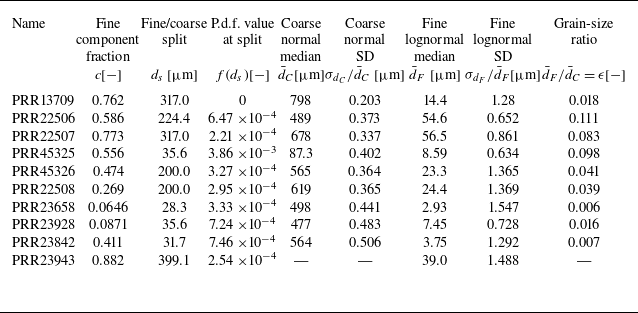

 +
 ×
 ◯
 △
 ◻
 x


 Open access

