1 Introduction
Large-scale collapse or transition to disorder of rapidly rotating contained flows with low-level periodic mechanical forcing has been reported in many experimental studies. Typically the forcing in such experiments has been created either by boundaries which move at a differential rotation rate (e.g. McEwan Reference McEwan1970; Malkus Reference Malkus1989) or by precession of the vessel about an axis other than the symmetry axis (e.g. Malkus Reference Malkus1968; Manasseh Reference Manasseh1992; Lagrange et al. Reference Lagrange, Eloy, Nadal and Meunier2008). Transition may occur rapidly following initiation of forcing.
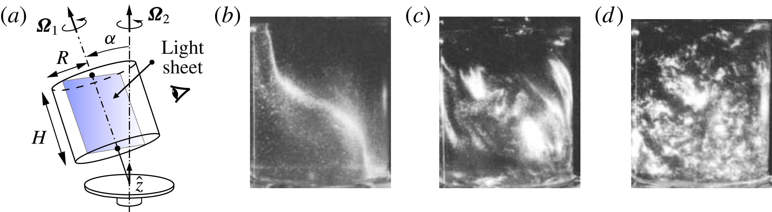
(a) Schematic of precessing flow configuration, and (b–d) rheoscopic flow visualizations of a ‘Type A collapse’ by Manasseh (Reference Manasseh1992, figure 5, see also supplementary movie 1 of the present work) at
 $Re=|\unicode[STIX]{x1D734}_{1}|R^{2}/\unicode[STIX]{x1D708}=21\,120$
: commencing from solid-body rotation about axis
 $\hat{\boldsymbol{z}}$
, the flow develops quasisteady three-dimensional structure (b) soon after tilting through angle
 $\unicode[STIX]{x1D6FC}=3^{\circ }$
; unsteady wavy instabilities are observed (c); followed by large-scale disorder (d).
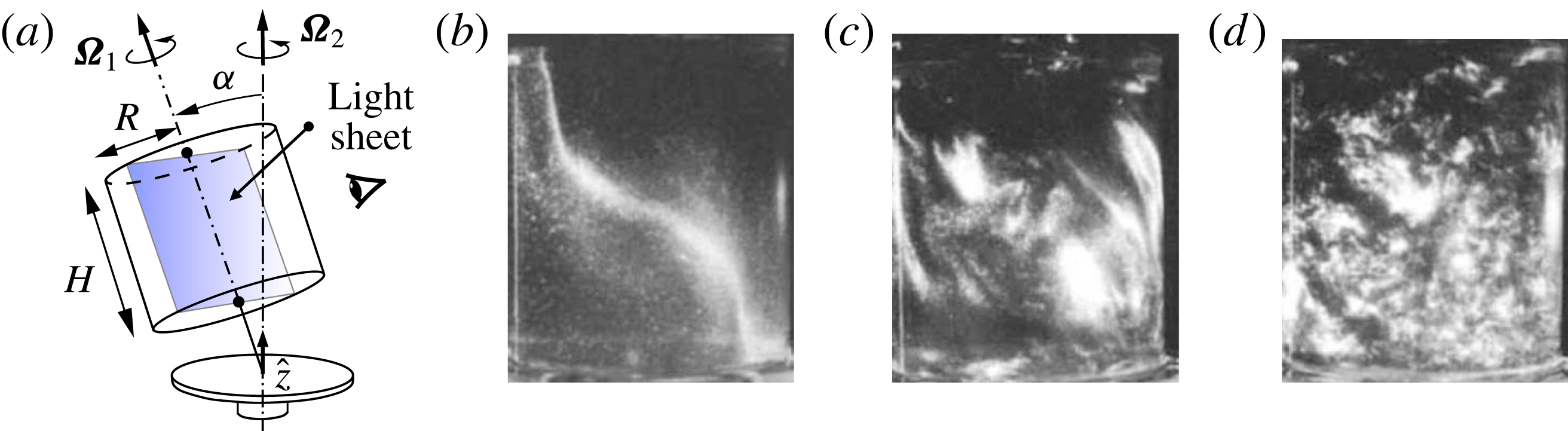
In most cases of interest, the vessel rotation rate about a symmetry axis is less than twice its total rotation rate in an inertial frame of reference. That is because, in these circumstances, inertial waves whose restoring force can alternatively be taken as caused by pressure gradients associated with solid-body rotation or by Coriolis effects can be driven near to or at resonance to reach moderately large amplitudes compared to the background rotation. The amplitudes of such forced waves are limited by nonlinear energy transfers and viscous damping, and, if stable, will saturate to outcomes which are stationary with respect to the forcing (and which are temporally periodic with respect to the vessel). However, as suggested above, these three-dimensional flows are themselves often unstable to further disturbances which are able to extract energy from the system and which may saturate either to even larger organized waves or make the transition to disordered states. This behaviour was originally studied in some depth by McEwan (Reference McEwan1970), who coined the phrase ‘resonant collapse’ for the transition, and subsequently by Manasseh (Reference Manasseh1992), whose observations of ‘Type A collapse’ in a precessing cylinder (see figure 1 and supplementary movie 1 available at https://doi.org/10.1017/jfm.2018.145) motivated the present work.
Two broad classes of instability in precessing cylinder flows have been noted, depending largely on whether the forcing is weak or strong. For weak forcing and near resonance of a low-order mode, behaviour consistent with weakly nonlinear systems emerges, characterized by the gradual and persistent appearance of modes of higher order that destabilize the forced mode, which Manasseh (Reference Manasseh1992) called a ‘Type B collapse’, and quasi-periodic recurrent instabilities with a similar appearance, which Manasseh called a ‘Type C collapse’. These weakly unstable limit-cycle and quasi-periodic behaviours have been reproduced numerically in our previous works (Albrecht et al. Reference Albrecht, Blackburn, Lopez, Manasseh and Meunier2015; Giesecke et al. Reference Giesecke, Albrecht, Gundrum, Herault and Stefani2015; Marques & Lopez Reference Marques and Lopez2015), and shown to result from triadic-resonance instability. However, for larger forcing, behaviour which apparently differed qualitatively was observed in Manasseh’s experiments. As may be seen in our accompanying supplementary movie 1 of rheoscopic flow visualization recorded during the course of those experiments, growth of instability proceeded rapidly from initial observation to very disordered states with fine-scale motions and little discernible structure other than large-scale overturning. Manasseh (Reference Manasseh1992) referred to this behaviour as a ‘Type A’ collapse. In the present work the geometry, frequency ratios and tilt angles employed are the same as for the ‘Type A’ collapse examined in § 4.3.2 of Manasseh (Reference Manasseh1992).
Our focus here is on the instability of a steady three-dimensional basic state (as in figure 1
b) on which unsteady three-dimensional features grow (figure 1
c). Stability analysis of such basic states is not straightforward, but as Kerswell (Reference Kerswell1993, Reference Kerswell1999, Reference Kerswell2002) relates, combinations of wave instabilities can satisfy triadic-resonance conditions with respect to the basic state, so that nonlinear product terms of the disturbance are able to lock to it, enabling extraction of energy into the other components of the triad. If the basic state has azimuthal wavenumber
 $m_{F}$
and angular frequency
 $\unicode[STIX]{x1D714}_{F}$
, then any two other modes which participate in a triadic resonance with it must satisfy
 $$\begin{eqnarray}|\!\pm m_{1}\pm m_{2}|=m_{F},\quad |\!\pm \unicode[STIX]{x1D714}_{1}\pm \unicode[STIX]{x1D714}_{2}|=\unicode[STIX]{x1D714}_{F}.\end{eqnarray}$$
Another contribution of Kerswell (Reference Kerswell1993) was to show that for inviscid flows in precessing spheroids, triadic-resonance instabilities associated both with
 $m_{F}=1$
and
 $m_{F}=2$
as predicted in the vessel frame of reference could alternatively be identified with Hopf bifurcations from a basic state that is steady in the gimbal/precessing frame of reference. In what follows we demonstrate that a similar relationship exists in instabilities of viscous flows contained in precessing cylinders.
While the real flows are viscous, Reynolds numbers are usually quite large at instability, prompting modellers to draw on the large body of theory associated with inviscid modes of rotating flows (Greenspan Reference Greenspan1968); in the context of cylindrical flows these are known as Kelvin modes, which have Fourier–Fourier–Bessel azimuthal–axial–radial spatial structure. (It is common in experiments to tune the geometry of the vessel and rotation rates to match resonance with a low-order Kelvin mode so that a large-amplitude three-dimensional structure can be achieved with a comparatively small forcing amplitude.) Using the concepts of triadic resonance, Kelvin modal structure, simple nonlinear models to estimate the amplitude of a low-order mode driven near resonance, and calibration to experiments, Eloy, Le Gal & Le Dizés (Reference Eloy, Le Gal and Le Dizés2003) developed reduced-order models for inertial-wave-type instabilities for periodically deformed rotating cylinders, while Meunier et al. (Reference Meunier, Eloy, Lagrange and Nadal2008), Lagrange et al. (Reference Lagrange, Meunier, Nadal and Eloy2011) extended application to precessing cylindrical containers. In experiments and direct numerical simulations (DNS) these models have been successful in predicting onset and structure of instabilities (Eloy et al.
Reference Eloy, Le Gal and Le Dizés2003; Lagrange et al.
Reference Lagrange, Eloy, Nadal and Meunier2008; Albrecht et al.
Reference Albrecht, Blackburn, Lopez, Manasseh and Meunier2015; Marques & Lopez Reference Marques and Lopez2015). Since two underlying assumptions of Kelvin-mode-based triadic instability models must be that the basic state, though three-dimensional, is not a large departure from solid-body rotation and that Reynolds numbers are large, it is not clear how well they will perform when these assumptions are violated. Moreover, the mechanism of triadic resonance as a possible instability mechanism for precessing cylinder flows remains controversial. On the basis of DNS studies of flows in precessing cylinders, Zhang & Liao (Reference Zhang and Liao2017) conclude their § 11.9 with the statement ‘It would seem reasonable to infer from the above result and argument that triadic resonance cannot take place in precessing cylinders at any precession angle
 $\unicode[STIX]{x1D6FC}$
and any aspect ratio
 $\unicode[STIX]{x1D6E4}$
.’
In the present work we examine DNS of precessing cylinder flows whose geometry and frequency ratios, tuned to closely coincide with resonance of the lowest-order three-dimensional Kelvin mode, match those for the ‘Type A’ collapse experiments of Manasseh (Reference Manasseh1992). As in that work, the system is not further tuned to satisfy any particular triadic-resonance condition. The Reynolds number used here is the lowest used in the experiments. First we compute unstable (steady, three-dimensional) basic states via selective frequency damping (SFD, Åkervik et al. Reference Åkervik, Brandt, Henningson, Hœpfner, Marxen and Schlatter2006), and show that these depart significantly from solid-body rotation for quite modest precessional nutation (tilt) angles. Allowing the flows to evolve from these basic states, one observes significant periods of initially uniform exponential growth of three-dimensional disturbances in all azimuthal Fourier modes in the simulation. The growth rates give saturation time scales comparable to those observed in experiments, despite the fact that Reynolds numbers of the DNS are typically smaller than those in the experiments. We employ dynamic mode decomposition (DMD, Schmid Reference Schmid2010; Jovanović, Schmid & Nichols Reference Jovanović, Schmid and Nichols2014) to analyse DNS data and show that there are two complementary ways of interpreting disturbance growth, either as a simple Hopf bifurcation or as a triadic resonance with a single group velocity, depending on which frame of reference is adopted. This strongly suggests that the instability mechanism leading to Manasseh’s ‘Type A’ collapse was of triadic resonance type. We examine how tilt angle (and hence departure from solid-body rotation) influences the leading modes of the disturbance, and show that the model of Lagrange et al. (Reference Lagrange, Meunier, Nadal and Eloy2011) successfully predicts onset of instability, growth rates and the leading triadic modes at small tilt angles, but overpredicts growth rates at larger tilt angles.
2 Problem definition and methodology
As represented in figure 1(a), we consider incompressible viscous flow of fluid that fills a cylinder of height
 $H$
and radius
 $R$
. The cylinder rotates around its axis with angular velocity
 $\unicode[STIX]{x1D734}_{1}$
with respect to the gimbal that attaches it to a turntable which in turn rotates with angular velocity
 $\unicode[STIX]{x1D734}_{2}$
about axis
 $\hat{\boldsymbol{z}}$
, fixed in an inertial frame of reference. The gimbal is tilted through nutation angle
 $\unicode[STIX]{x1D6FC}$
so that the axis of the cylinder precesses with respect to the inertial frame. We define the cylinder rotation rate
 $\unicode[STIX]{x1D6FA}_{1}=|\unicode[STIX]{x1D734}_{1}|\operatorname{sgn}(\unicode[STIX]{x1D734}_{1}\boldsymbol{\cdot }\hat{\boldsymbol{z}})$
to be positive and
 $\unicode[STIX]{x1D6FA}_{2}=|\unicode[STIX]{x1D734}_{2}|\operatorname{sgn}(\unicode[STIX]{x1D734}_{2}\boldsymbol{\cdot }\hat{\boldsymbol{z}})$
.
Precession drives the flow away from the solid-body rotation which would exist for
 $\unicode[STIX]{x1D6FC}=0$
. In the inertial frame, the forcing is created by periodic precessional motion of the cylinder walls, but these flows are more readily considered in rotating frames of reference in which the cylinder geometry appears fixed. We note that there are two canonical such rotating frames. The first is the gimbal (or precessing) frame of reference, in which the cylinder walls rotate steadily and in which the precessional forcing is fixed with respect to the frame, making it possible to find a steady solution to the Navier–Stokes equations. The second canonical case is the cylinder frame of reference, in which the walls of the cylinder as well as its geometry appear fixed, but the precessional forcing rotates steadily. Most of the previous theoretical considerations of the fluid motion are cast in the cylinder frame, while most laboratory measurements and visualizations of such flows are obtained from the gimbal frame. In a numerical study one is free to consider the flow in either frame, and part of our purpose here is to show what can be learned by examining the arising flow instabilities in each frame.
Similar to our earlier work (Albrecht et al. Reference Albrecht, Blackburn, Lopez, Manasseh and Meunier2015), a cylindrical formulation of the incompressible Navier–Stokes equations written for a rotating frame
 $$\begin{eqnarray}\unicode[STIX]{x2202}\boldsymbol{u}/\unicode[STIX]{x2202}t+\boldsymbol{u}\boldsymbol{\cdot }\unicode[STIX]{x1D735}\boldsymbol{u}+2\unicode[STIX]{x1D734}\times \boldsymbol{u}+(\text{d}\unicode[STIX]{x1D734}/\text{d}t)\times \boldsymbol{r}=-\unicode[STIX]{x1D735}p+Re^{-1}\unicode[STIX]{x1D6FB}^{2}\boldsymbol{u}-\unicode[STIX]{x1D712}(\boldsymbol{u}-\overline{\boldsymbol{u}}),\quad \unicode[STIX]{x1D735}\boldsymbol{\cdot }\boldsymbol{u}=0,\end{eqnarray}$$
is solved using a spectral element–Fourier method (Blackburn & Sherwin Reference Blackburn and Sherwin2004, source code available at http://users.monash.edu.au/∼bburn/semtex.html), with no-slip boundary conditions on all cylinder walls. One can compute (2.1) in either of the two canonical frames and then if required transform between them by adding or subtracting solid-body rotation. In the cylinder frame
 $\unicode[STIX]{x1D734}=\unicode[STIX]{x1D734}_{1}+\unicode[STIX]{x1D734}_{2}(t)$
varies with time, whereas in the gimbal frame it is steady,
 $\unicode[STIX]{x1D734}=\unicode[STIX]{x1D734}_{2}$
. Hence, we focus on working in the gimbal frame because there it is possible to find steady solutions to (2.1) since
 $\text{d}\unicode[STIX]{x1D734}/\text{d}t=\mathbf{0}$
.
To compute unstable steady solutions, we adopt the selective frequency damping (SFD) approach of Åkervik et al. (Reference Åkervik, Brandt, Henningson, Hœpfner, Marxen and Schlatter2006), in which a penalty term of the form
 $-\unicode[STIX]{x1D712}(\boldsymbol{u}-\overline{\boldsymbol{u}})$
appears in the momentum equation of (2.1) and where the estimate of the time-mean flow
 $\overline{\boldsymbol{u}}$
is updated using forwards-Euler integration as computation proceeds towards a steady state, with
 $\unicode[STIX]{x1D712}=0.1$
and a filter width
 $\unicode[STIX]{x1D6E5}=25/\unicode[STIX]{x03C0}$
(c.f. Åkervik et al. equation (6)). This penalization counteracts the
 $\unicode[STIX]{x2202}\boldsymbol{u}/\unicode[STIX]{x2202}t$
term in (2.1), tending to stabilize the solutions towards a steady outcome, though since the approximation to
 $\unicode[STIX]{x2202}\boldsymbol{u}/\unicode[STIX]{x2202}t$
is inexact the outcomes are only an approximation to the steady version of (2.1). When
 $\unicode[STIX]{x2202}\boldsymbol{u}/\unicode[STIX]{x2202}t=0$
to within a small tolerance,
 $\overline{\boldsymbol{u}}$
is saved as the basic state and we change
 $\unicode[STIX]{x1D712}$
from
 $0.1\rightarrow 0$
in order to allow potential instabilities to evolve. The perturbation flow
 $\boldsymbol{u}^{\prime }=\boldsymbol{u}-\overline{\boldsymbol{u}}$
is then computed in postprocessing.
A convenient diagnostic measure of solutions is the amount of kinetic energy in each azimuthal Fourier mode,
 $$\begin{eqnarray}E_{m}=(2A)^{-1}\int _{A}\widehat{\boldsymbol{u}}_{m}\boldsymbol{\cdot }\widehat{\boldsymbol{u}}_{m}^{\ast }\,r\,\text{d}A,\end{eqnarray}$$
where
 $A$
is the area of the meridional semiplane,
 $r$
is radius and
 $\widehat{\boldsymbol{u}}_{m}^{\ast }$
represents the complex conjugate of azimuthal mode
 $m$
of the Fourier transform of
 $\boldsymbol{u}$
. We use
 $\overline{E}_{m}$
when the velocity field is
 $\overline{\boldsymbol{u}}$
, the steady-state solution of (2.1) and
 $E_{m}^{\prime }$
when the velocity field is the perturbation
 $\boldsymbol{u}^{\prime }=\boldsymbol{u}-\overline{\boldsymbol{u}}$
, all as measured in the gimbal frame of reference. To show relative significance, these energies are typically normalized by
 $E_{SBR}$
, the kinetic energy of solid-body rotation at speed
 $r\unicode[STIX]{x1D6FA}_{1}$
.
There are four independent dimensionless control parameters, which we take as the cylinder aspect ratio
 $\unicode[STIX]{x1D6E4}=H/R$
, tilt angle
 $\unicode[STIX]{x1D6FC}$
, Reynolds number
 $Re=\unicode[STIX]{x1D6FA}_{1}R^{2}/\unicode[STIX]{x1D708}$
and dimensionless forcing frequency
 $\unicode[STIX]{x1D714}_{F}$
. For the latter, we follow Meunier et al. (Reference Meunier, Eloy, Lagrange and Nadal2008) and Lagrange et al. (Reference Lagrange, Meunier, Nadal and Eloy2011) and define
 $\unicode[STIX]{x1D714}_{F}=\unicode[STIX]{x1D6FA}_{1}/(\unicode[STIX]{x1D6FA}_{1}+\unicode[STIX]{x1D6FA}_{2}\cos \unicode[STIX]{x1D6FC})$
, i.e. the cylinder’s angular velocity with respect to the turntable, non-dimensionalized by the total angular velocity with respect to the inertial frame. We note that another dimensionless parameter, the Poincaré number
 $Po=\unicode[STIX]{x1D6FA}_{1}/\unicode[STIX]{x1D6FA}_{2}$
, is sometimes employed. This is useful because the strength of the precessional forcing is proportional to
 $|Po|\sin \unicode[STIX]{x1D6FC}$
. Thus it is possible to have a large tilt angle yet a small precessional forcing. In the present work,
 $Po=0.361$
.
As mentioned in § 1, the parameters
 $\unicode[STIX]{x1D6E4}=2.667$
,
 $\unicode[STIX]{x1D714}_{F}=2/2.72=0.735$
have been chosen to match work described in Manasseh (Reference Manasseh1992). The results reported here are for
 $Re=4778$
, the lowest value used by Manasseh, and the tilt angle is varied up to
 $\unicode[STIX]{x1D6FC}_{max}=3^{\circ }$
, which was found sufficient to produce a rapid ‘Type A’ collapse (§ 4.3.2, Manasseh Reference Manasseh1992).
We have used 192 quadrilateral elements to mesh the meridional semiplane, with significant refinement near the side and end walls (see figure 3 of Albrecht et al. Reference Albrecht, Blackburn, Meunier, Manasseh and Lopez2016, for a comparable mesh), and employed up to 64 azimuthal Fourier modes (128 planes of real data) for the largest tilt angles. We will briefly describe resolution studies in § 4.
3 Basic states
Basic states
 $\overline{\boldsymbol{u}}$
are fixed in the gimbal frame of reference but rotate steadily at
 $-\unicode[STIX]{x1D6FA}_{1}$
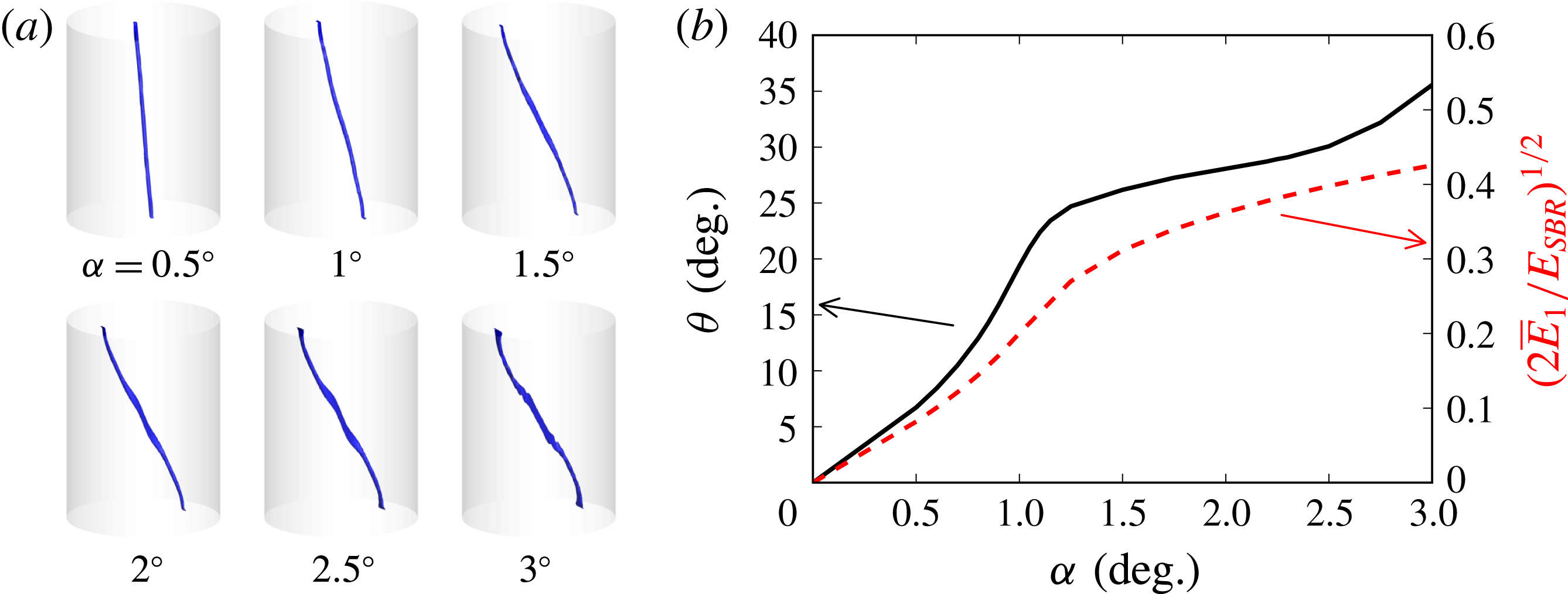
in the cylinder frame of reference. Outcomes are summarized in figure 2, where figure 2(a) shows how vortex-core geometry (here defined as an isosurface of flow speed that is 1% of the maximum) varies with tilt angle – these results may be compared with the visualization of figure 1(b). Clearly the flow departs significantly from solid-body rotation, becoming more three-dimensional with increasing tilt angle. Also clear is that the flow remains well organized around a curvilinear vortex core. Near the end walls, this core is displaced substantially from the axis of symmetry. For the highest tilt angles, slight kinks may be observed in the vortex core near the midheight of the cylinder, an effect which is associated with the presence of inertial wave beams that emanate near the intersection of the cylinder’s side and end walls. Note that in precessing cylinder flows, such beams are not conical owing to the
 $m=1$
forcing. We refer the reader to Marques & Lopez (Reference Marques and Lopez2015), Lopez & Marques (Reference Lopez and Marques2018) for more detail concerning such basic states.
(a) Vortex core of the basic states visualized by isosurfaces of
 $|\overline{\boldsymbol{u}}|/\max (|\overline{\boldsymbol{u}}|)=0.01$
. (b) The angle
 $\unicode[STIX]{x1D703}$
between the vortex core and the cylinder axis at the centroid of the cylinder, and
 $(2\overline{E}_{1}/E_{SBR})^{1/2}$
, measures of flow three-dimensionality, both as functions of tilt angle
 $\unicode[STIX]{x1D6FC}$
.
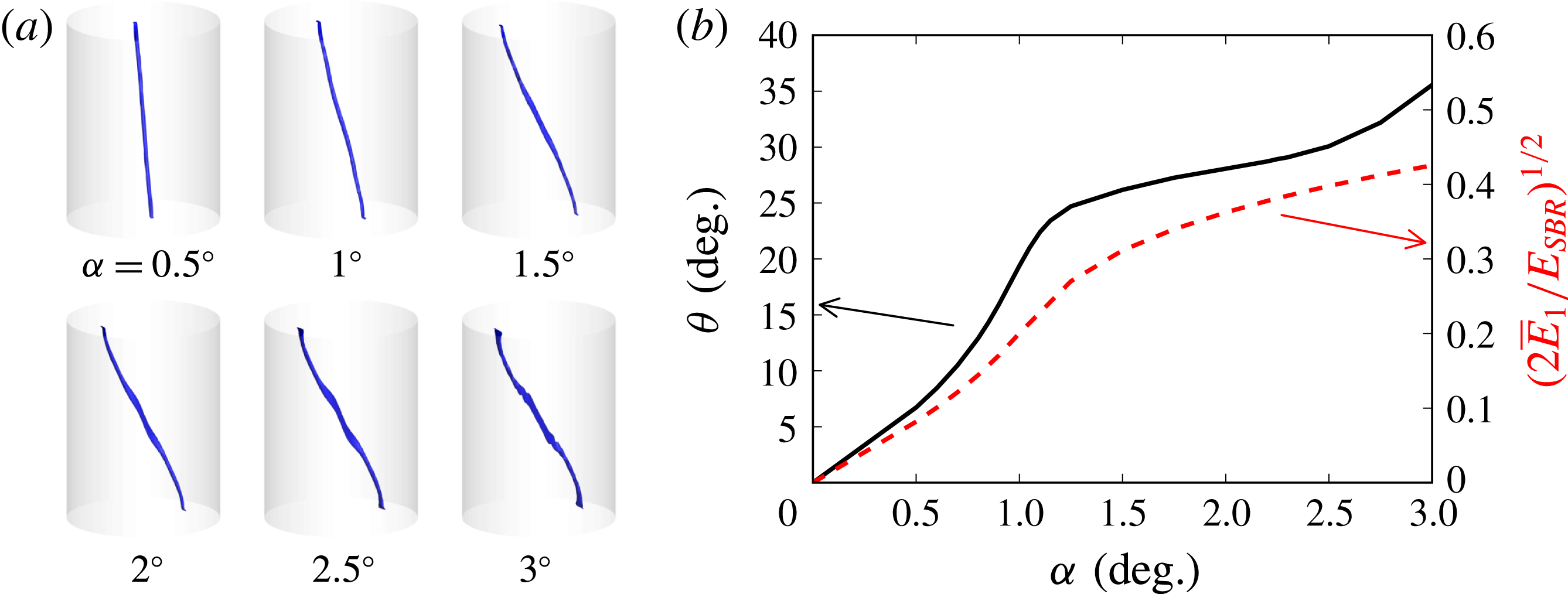
Figure 2(b) shows quantitative measures of flow three-dimensionality extracted from the basic states. The first measure is the angle
 $\unicode[STIX]{x1D703}$
made between the centreline of the vortex-core extractions shown in figure 2(a) and the cylinder axis, at the centroid of the cylinder. The angle increases monotonically with
 $\unicode[STIX]{x1D6FC}$
, though the rate of increase declines near
 $\unicode[STIX]{x1D6FC}=1^{\circ }$
, when kinks on the vortex core start to become significant. To quantify the relative significance of the resonant three-dimensional flow compared to the background solid-body flow component, the measure
 $(2\overline{E}_{1}/E_{SBR})^{1/2}$
is also shown in figure 2(b); the leading factor of 2 owes to contributions in
 $m=\pm 1$
. This ratio, like
 $\unicode[STIX]{x1D703}$
, also increases monotonically with
 $\unicode[STIX]{x1D6FC}$
, to reach a peak value of approximately 40% at
 $\unicode[STIX]{x1D6FC}=3^{\circ }$
, again indicating that the basic state is substantially three-dimensional. The departure from solid-body rotation is dominated by azimuthal wavenumber
 $m_{F}=1$
, and in the cylinder frame, by frequency
 $\unicode[STIX]{x1D714}_{F}$
, thus setting the stage for triadic resonances according to (1.1).
4 Instabilities of the basic state
Figure 3 shows the evolution of
 $E_{m}^{\prime }/E_{SBR}$
following removal at
 $t=0$
of SFD penalization for
 $\unicode[STIX]{x1D6FC}=3^{\circ }$
; additional simulations have been carried out for a range of lower tilt angles, but are not represented in the figure, since they all, if unstable (cf. figure 6
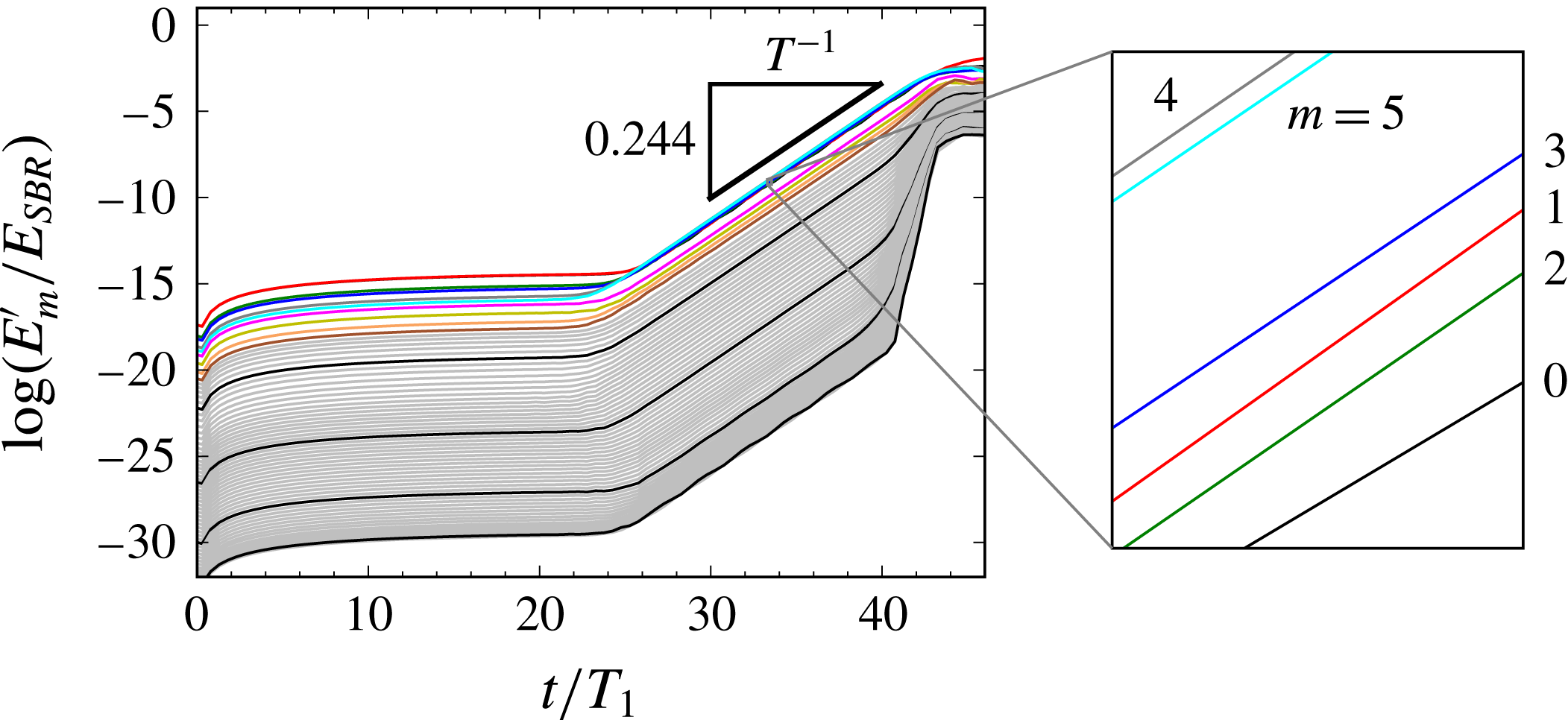
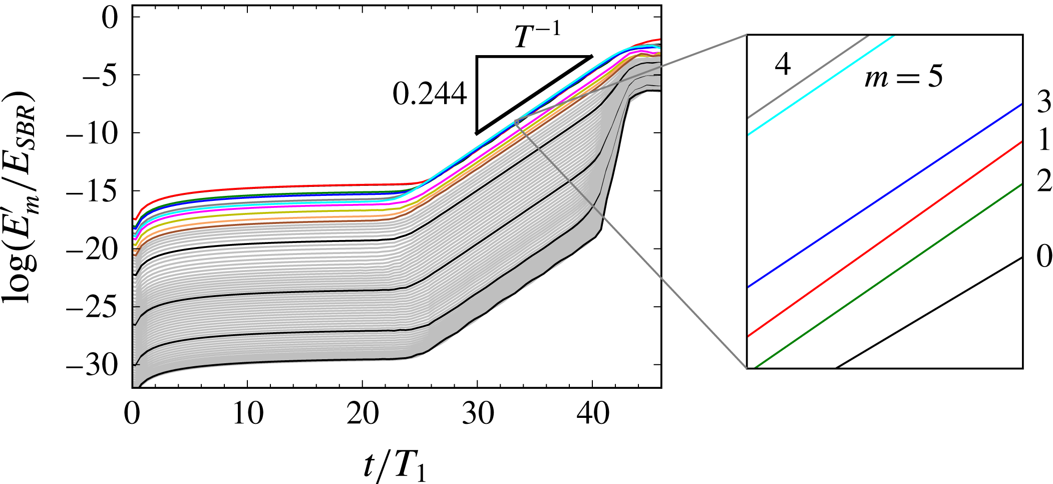
a), exhibit the same qualitative behaviour. Initial modal energies, though very small, are never exactly zero owing to the fact that, as explained in § 2, the SFD-penalized Navier–Stokes equations are an approximation to the steady Navier–Stokes equations. The paramount feature of figure 3(a) is that after some elapsed time, associated with the time required for instabilities to grow above background levels, disturbances in all Fourier modes grow exponentially at the same rate until saturation is approached at
 $t/T_{1}>40$
, where
 $T_{1}=2\unicode[STIX]{x03C0}/\unicode[STIX]{x1D6FA}_{1}$
. (Similar behaviour, but with weaker growth owing to smaller values of
 $|Po|\sin \unicode[STIX]{x1D6FC}$
, was apparent in our earlier work dealing with triadic-resonance instability – see figures 2 and 7 of Albrecht et al. (Reference Albrecht, Blackburn, Lopez, Manasseh and Meunier2015), although attention was there confined to only the leading Fourier modes engaged in those instabilities, and to agreement with the reduced-order model for growth of leading Kelvin modes by Lagrange et al. (Reference Lagrange, Meunier, Nadal and Eloy2011)). Figure 3 shows that at
 $\unicode[STIX]{x1D6FC}=3^{\circ }$
, disturbance energies grow by 12 orders of magnitude to reach saturation in approximately 20 cylinder revolutions.
History of Fourier modal energies in the disturbance flow
 $\boldsymbol{u}^{\prime }$
for
 $\unicode[STIX]{x1D6FC}=3^{\circ }$
,
 $Re=4778$
. The thick black triangle indicates the period over which DMD analysis was performed, as well as the growth rate. Ordering of leading Fourier modes during the growth phase is shown in the zoomed-in region; at earlier times, the two leading modes were
 $m=1$
and
 $m=0$
.
We have computed flows using a variety of discretization levels, but always with the same 192-spectral-element decomposition of the meridional semiplane. The basic resolution used to obtain the presented results used spectral element shape functions that were tensor products of sixth-order Lagrange interpolants and 64 azimuthal Fourier modes. A reduction to fourth-order interpolants and 32 Fourier modes changed the growth rates by at most 1%, leaving the overall dynamics otherwise the same.
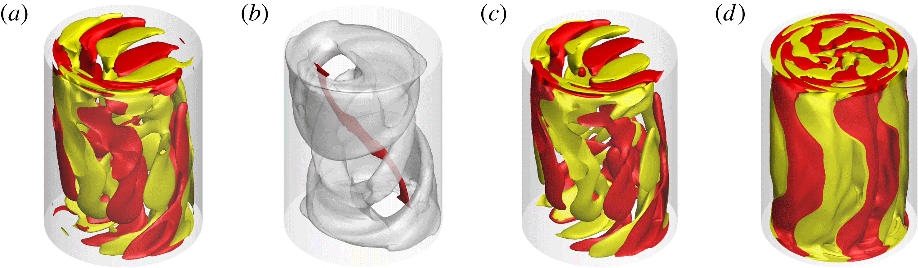
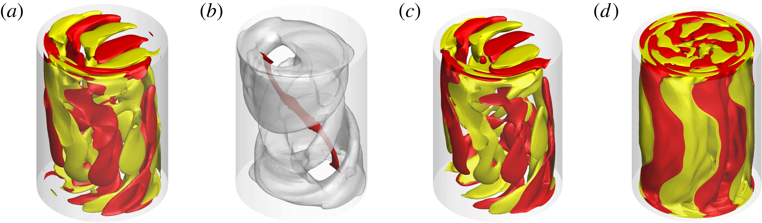
Flow visualization and animation has been central to developing our understanding of flow physics in this problem. Figure 4(a) shows a perspective view of isosurfaces of axial vorticity in the perturbation flow
 $\boldsymbol{u}^{\prime }$
for
 $\unicode[STIX]{x1D6FC}=3^{\circ }$
at
 $t/T_{1}=35.738$
, after exponential growth is established (cf. figure 3). This view suggests that the disturbance takes the form of a three-dimensional wave that is aligned around the vortex-core base-flow structure seen in figure 2(a), which is steady in the gimbal frame of reference. In order to focus on wave structure, it has been helpful in preparing animations to first normalize the velocity snapshots in order to remove the growth observed in figure 3. Two such animations of axial vorticity for the
 $\unicode[STIX]{x1D6FC}=3^{\circ }$
case are provided as supplementary movies 2 and 3; movie 2 provides an animation as seen from the gimbal frame of reference, while movie 3 is of the same data but visualized from the cylinder frame of reference. In movie 2 it is evident that the wave envelope remains steady with respect to the gimbal frame (and the basic state), but there is a dominant frequency associated with progress of the wave; this is the phase frequency of the wave in the gimbal frame. In movie 3, the whole wave as well as the basic state revolve at circular frequency
 $\unicode[STIX]{x1D6FA}_{1}$
with respect to the observer. From the normalized snapshots used to create movie 2, the time-average kinetic energy has been computed; an isosurface of this quantity shown in figure 4(b) illustrates how the wave envelope coils around the vortex core of the basic state.
Structure of the instability for
 $\unicode[STIX]{x1D6FC}=3^{\circ }$
. (a) Instantaneous
 $\pm$
isosurfaces of perturbation axial vorticity at
 $t/T_{1}=35.738$
(figure 3); see also supplementary movies 2 and 3. (b) Translucent isosurface of time-average perturbation kinetic energy (after de-trending for exponential growth), superimposed over the vortex core of the basic state. Also shown are isosurfaces of axial vorticity for the leading DMD modes from (c) gimbal-frame and (d) cylinder-frame analyses.
Dynamic mode decomposition (DMD, Schmid Reference Schmid2010) can be used to approximate a temporally evolving flow field with a sum of spatial modes
 $\unicode[STIX]{x1D74D}_{j}(\boldsymbol{x})$
of constant shape;
 $$\begin{eqnarray}\boldsymbol{u}(\boldsymbol{x},t)\approx \mathop{\sum }_{j}a_{j}\text{e}^{(\unicode[STIX]{x1D70E}_{j}+\text{i}\unicode[STIX]{x1D714}_{j})t}\unicode[STIX]{x1D74D}_{j}(\boldsymbol{x}),\end{eqnarray}$$
each
 $\unicode[STIX]{x1D74D}_{j}$
being associated with a unique frequency
 $\unicode[STIX]{x1D714}_{j}$
and growth rate
 $\unicode[STIX]{x1D70E}_{j}$
(both real), and complex amplitude
 $a_{j}$
. Since the original data are real, DMD modes occur in complex-conjugate pairs at
 $\pm \unicode[STIX]{x1D714}_{j}$
. The procedure operates on uniformly sampled snapshots
 $\boldsymbol{v}_{j}$
of the flow field, which are assumed to form a Krylov sequence
 $\boldsymbol{V}=\left\{\boldsymbol{v}_{1},\boldsymbol{A}\boldsymbol{v}_{1},\boldsymbol{A}^{2}\boldsymbol{v}_{1},\ldots ,,\boldsymbol{A}^{N-1}\boldsymbol{v}_{1}\right\}$
i.e. subsequent snapshots are connected by a constant linear mapping
 $\boldsymbol{A}$
. We used the sparsity-promoting variant of DMD (Jovanović et al.
Reference Jovanović, Schmid and Nichols2014; Horn & Schmid Reference Horn and Schmid2017), which minimizes the number of modes required to recover the snapshot sequence to within a specified accuracy. DMD may be based on snapshots of any flow variable; we have used perturbation axial vorticity computed in postprocessing, as a scalar field derived from
 $\boldsymbol{u}^{\prime }$
. We note that DMD analysis makes no assumption regarding spatial structure of modes. We have used it on snapshot sequences from time windows clearly associated with exponential growth (see figure 3), so that one expects leading DMD modes – those with largest
 $|a_{j}|$
– to have
 $\unicode[STIX]{x1D70E}_{j}$
matching (one-half) the observed growth in
 $E_{m}^{\prime }$
.
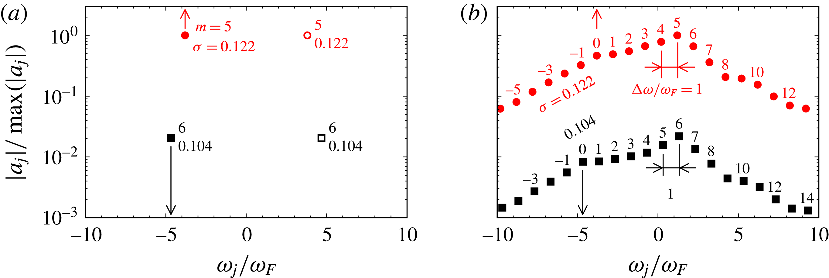
Analyses have been computed in both gimbal and cylinder frames of reference, and we present in figure 5 information from the two leading sets of DMD modes in each frame, as computed for
 $\unicode[STIX]{x1D6FC}=3^{\circ }$
. In each plot, the modal amplitudes are normalized such that
 $|a_{j}|_{max}=1$
. Figure 5(a) shows outcomes for the gimbal-frame DMD; the spectrum of
 $|a_{j}|$
versus dimensionless frequency
 $\unicode[STIX]{x1D714}/\unicode[STIX]{x1D714}_{F}$
shows four modes: two sets of complex-conjugate pairs at
 $\pm \unicode[STIX]{x1D714}/\unicode[STIX]{x1D714}_{F}$
. The growth rate
 $\unicode[STIX]{x1D70E}_{\pm 1}=0.122$
associated with the leading pair of modes,
 $a_{\pm 1}$
, matches (one-half) the energy growth rate for all Fourier modes observed in figure 3. The other pair of instability modes represented in figure 5(a) has a lower growth rate,
 $\unicode[STIX]{x1D70E}_{\pm 2}=0.104$
, and amplitude
 $|a_{\pm 2}|\ll |a_{\pm 1}|$
. Each of these pairs of modes can be ascribed to a Hopf bifurcation from the basic state, which is steady in the gimbal frame of reference. The frequency of each of these Hopf modes corresponds to the motion of wavepacket features, seen in figure 4(a) and supplementary movie 2, i.e. it is associated with the phase velocity of wavepackets as observed in the gimbal frame (but since the frequencies are close, and
 $|a_{\pm 1}|\gg |a_{\pm 2}|$
, it is difficult to distinguish the two). Since the saturation levels of
 $E_{m}^{\prime }$
in figure 3 are approached with monotonically declining growth rates in the leading modes, the Hopf bifurcations are supercritical.
Amplitude–frequency spectra for DMD analyses at
 $\unicode[STIX]{x1D6FC}=3^{\circ }$
carried out in (a) the gimbal frame of reference and (b) the cylinder frame of reference. Each data point represents a DMD mode, with numeric labels representing the azimuthal wavenumber
 $m$
of the mode shape, and its growth rate
 $\unicode[STIX]{x1D70E}$
. Each DMD mode represented on (a) corresponds to a ‘triad tree’ of modes on (b) that share the same symbol and growth rate. In (a) the supplied values of
 $m$
represent the dominant azimuthal wavenumber of the DMD mode, while in (b) the values of
 $m$
are precise for each mode. In order to reduce clutter, only one-half of the complex-conjugate pairs of modes are represented in (b).
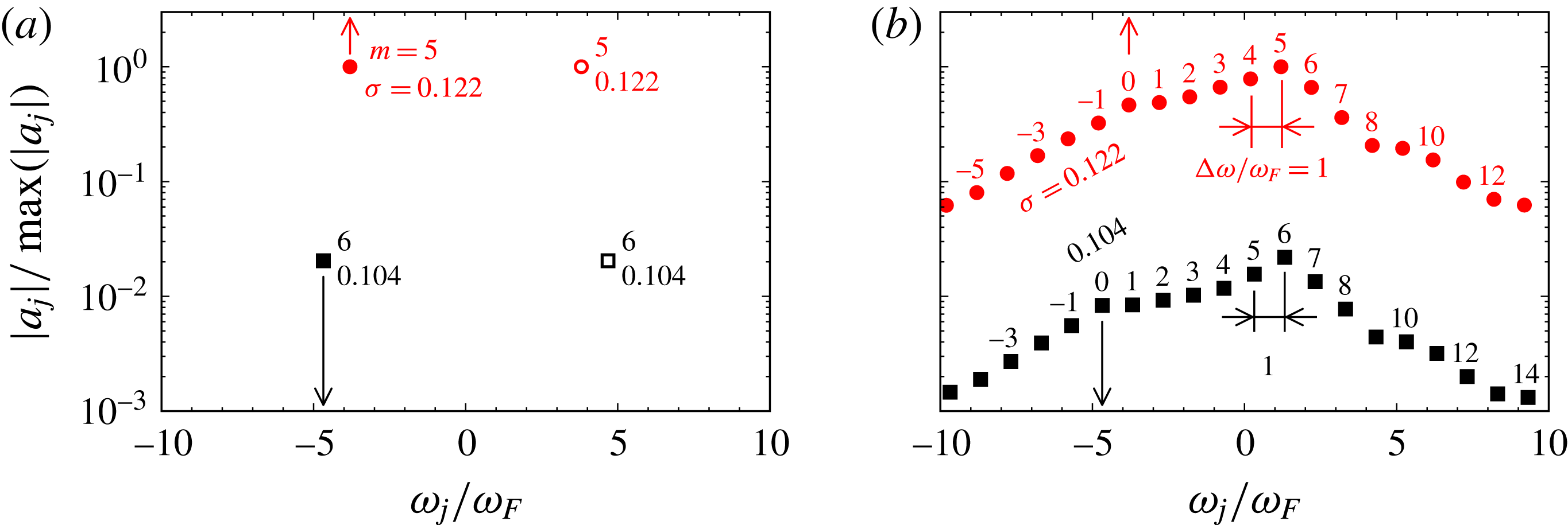
Figure 5(b) presents outcomes of DMD analysis based on snapshots rotated into the cylinder frame of reference. For clarity only one-half of the
 $|a_{j}|$
data are shown; for each point shown, there is a corresponding point at the negative value of
 $\unicode[STIX]{x1D714}/\unicode[STIX]{x1D714}_{F}$
that has been omitted. For each
 $|a_{j}|$
in the right-half-plane of figure 5(a), there is now a ‘triad tree’ of
 $|a_{j}|$
in figure 5(b). For each such tree, all DMD modes have the same value of
 $\unicode[STIX]{x1D70E}$
, which matches that of a corresponding Hopf mode in figure 5(a). For each
 $|a_{j}|$
, a numeric label shows the dominant azimuthal wavenumber of the spatial structure for the associated DMD mode
 $\unicode[STIX]{x1D713}_{j}$
. For gimbal-frame DMD modes, a variety of azimuthal wavenumbers contribute to each mode and its spectrum is somewhat broad, but cylinder-frame analysis generates an azimuthal Fourier decomposition, and each mode has a very sharp spectrum. This feature can be seen in the mode shapes for the leading DMD modes in figures 4(c) and (d), respectively for gimbal-frame and cylinder-frame analyses. The leading mode for the gimbal-frame analysis is visually similar to the DNS snapshot in figure 4(a) and has a complicated azimuthal structure dominated by
 $m=5$
, whereas the leading mode for the cylinder-frame analysis is very clearly almost pure
 $m=5$
(note also that it does not show any structural alignment with the vortex core of the basic state).
Three key features emerge for the analysis represented in figure 5(b). First, the frequency for each adjacent pair of modes in each tree differs by
 $|\unicode[STIX]{x1D6E5}(\unicode[STIX]{x1D714}/\unicode[STIX]{x1D714}_{F})|=1$
. Second, the azimuthal wavenumbers for each adjacent pair of modes in each tree also differ by unity, thus all the adjacent modes in each tree satisfy the triad conditions (1.1). Third, as a consequence, each tree of DMD modes is characterized by
 $\unicode[STIX]{x1D6E5}(\unicode[STIX]{x1D714}/\unicode[STIX]{x1D714}_{F})/\unicode[STIX]{x1D6E5}(m)=1$
, i.e. they share a common group velocity which is also the value required to keep the wavepacket rotating at the cylinder rotation rate, i.e. at a fixed orientation with respect to the basic state, which in the cylinder frame of reference is a rotating feature. Since the modes in each tree share a common growth rate and group velocity as well as satisfying (1.1), one may consider that a whole tree represents a single ‘generalized triad’.
One may note an exact correspondence between the two Hopf mode frequencies shown in the left-half-plane of figure 5(a) and the
 $m=0$
frequencies in the two triad trees of figure 5(b). Indeed (though not shown), the
 $m=0$
projection of the DMD modes found in the gimbal-frame analysis for figure 5(a) have the same spatial distributions as the DMD modes labelled
 $m=0$
for the two triad trees of figure 5(b). This is a consequence of the change of reference frame between analyses; only
 $m=0$
components can remain invariant in both frequency and shape under the rotational transformation.
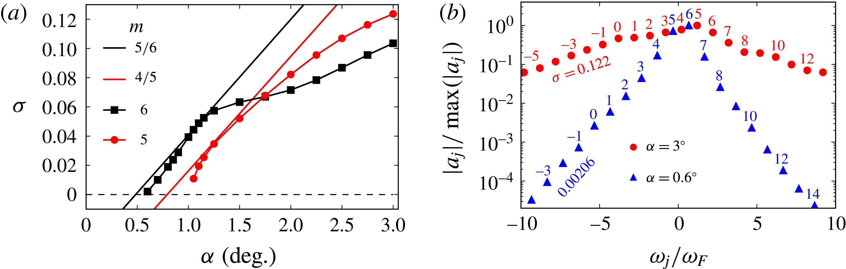
(a) Growth rates
 $\unicode[STIX]{x1D70E}$
of the two leading Hopf modes as functions of tilt angle
 $\unicode[STIX]{x1D6FC}$
(lines with symbols), with their dominant azimuthal wavenumbers
 $m$
, together with growth rates and triad wavenumbers obtained from the model of Lagrange et al. (Reference Lagrange, Meunier, Nadal and Eloy2011). (b) Leading triad trees from cylinder-frame analyses at
 $\unicode[STIX]{x1D6FC}=0.6^{\circ }$
and
 $3^{\circ }$
, with azimuthal wavenumbers and growth rates.
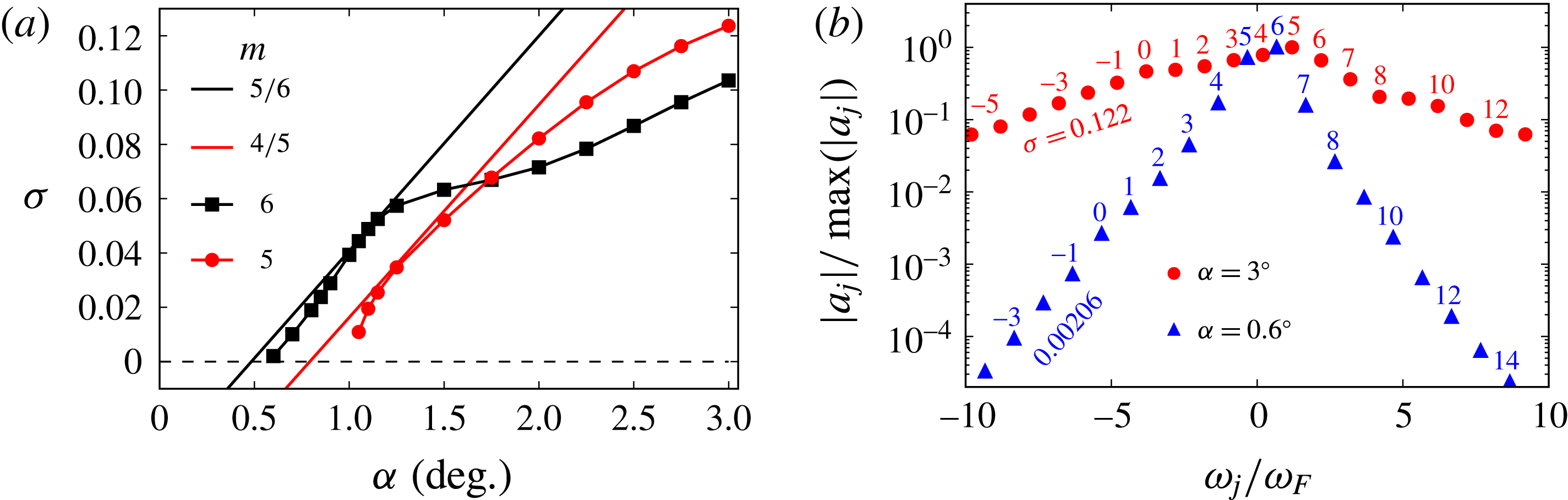
Figure 6(a) shows growth rates
 $\unicode[STIX]{x1D70E}$
of the two leading sets of DMD modes as a function of tilt angle
 $\unicode[STIX]{x1D6FC}$
. This suggests that the progression of instability dynamics in this system may be interpreted as a sequence of Hopf bifurcations from the basic state, a first which occurs near
 $\unicode[STIX]{x1D6FC}=0.6^{\circ }$
and a second near
 $\unicode[STIX]{x1D6FC}=1^{\circ }$
. At
 $\unicode[STIX]{x1D6FC}=1.7^{\circ }$
the growth rate of the second-bifurcating branch exceeds that of the first. Also shown on that figure are lines representing growth rates predicted by the model of Lagrange et al. (Reference Lagrange, Meunier, Nadal and Eloy2011) in this system (which as remarked in § 1 is not precisely tuned to any particular triad) for two different triadic interactions with the lowest-order three-dimensional Kelvin mode. While agreement is not perfect, the model performs well in predicting critical
 $\unicode[STIX]{x1D6FC}$
values, initial rise in growth rate with
 $\unicode[STIX]{x1D6FC}$
, and the leading azimuthal wavenumbers for each solution branch, which according to figure 5(b) are
 $m=4,5$
for the leading branch, and
 $m=5,6$
for the subdominant (at
 $\unicode[STIX]{x1D6FC}=3^{\circ }$
) but first-bifurcating branch in figure 6(a).
Figure 6(b), comparing the leading triad trees for cylinder-frame analyses at
 $\unicode[STIX]{x1D6FC}=0.6^{\circ }$
and
 $3.0^{\circ }$
(the latter reproduced from figure 5 b), shows the effect of tilt angle on the structure of a triad tree. As tilt angle reduces towards the critical value (
 $\unicode[STIX]{x1D6FC}_{c}=0.57^{\circ }$
, as compared to
 $0.48^{\circ }$
predicted by Lagrange et al. (Reference Lagrange, Meunier, Nadal and Eloy2011)) a tree becomes increasingly dominated by the fundamental triad modes (for
 $\unicode[STIX]{x1D6FC}=0.6^{\circ }$
these have
 $m=5$
and
 $m=6$
). This behaviour helps explain why the Lagrange et al. (Reference Lagrange, Meunier, Nadal and Eloy2011) model, which only considers the three fundamental Kelvin modes in a triad, is so successful at predicting critical values and initial increase of growth rates with
 $\unicode[STIX]{x1D6FC}$
.
5 Discussion and conclusions
As outlined in § 1, the present study has sought to examine the nature of resonant collapse in a system whose geometry, frequencies and maximum tilt angles matched those used in § 4.3.2 of Manasseh (Reference Manasseh1992). At
 $\unicode[STIX]{x1D6FC}=3^{\circ }$
,
 $Re=21\,210$
, ‘Type A’ collapses in Manasseh’s experiments proceeded rapidly to completion, and it would typically take
 $O(5)$
cylinder revolutions between visual observation of a wavy instability and saturation. This is similar to the number of cylinder revolutions required for energy of a disturbance to grow exponentially by three orders of magnitude in the present corresponding DNS. While our
 $Re=4778$
is lower, we note that the initiation-to-saturation time scales recorded in figure 4 of Manasseh (Reference Manasseh1992) are relatively insensitive to Ekman (inverse Reynolds) number.
From § 3 it is clear that the basic states obtained as
 $\unicode[STIX]{x1D6FC}\rightarrow 3^{\circ }$
are substantially three-dimensional such that it might be ambitious to assume validity of triadic-resonance models based on small departures from solid-body rotation (e.g. Lagrange et al.
Reference Lagrange, Meunier, Nadal and Eloy2011). Dynamics obtained from DNS suggest that the departure of observed growth rates from those predicted by the Lagrange et al. model occurs smoothly with increasing tilt angle and difference sets in once other Hopf modes (also predicted) bifurcate from the basic state. The model is shown to be broadly successful in the present circumstances (where the geometry and frequencies were not precisely tuned to a particular triad) in that it well predicts the critical tilt angle for instability, the nature of the modes involved, and the initial variation in growth rate with tilt angle. At larger tilt angles however, the model substantially overpredicts growth rates compared to observed values.
In summary, we suggest that this study demonstrates that the instability mechanism associated with the violent ‘Type A’ resonant collapse observed by Manasseh (Reference Manasseh1992) is of triadic type, in common with (at least) Types B and C, but that the dynamics become richer, and growth rates larger, with increasing forcing amplitudes. We have shown that, considered in an alternative frame of reference in which the basic state is steady (here, the gimbal frame), such instabilities are of Hopf type. At
 $\unicode[STIX]{x1D6FC}>1.1^{\circ }$
here, the basic state is unstable to two different Hopf modes, allowing more complex behaviour; for
 $\unicode[STIX]{x1D6FC}>1.7^{\circ }$
the second-bifurcating Hopf has larger growth rate than the first. Fundamentally, the nature of the instability is exactly the same regardless of the frame of reference used. The distinction between outcomes of, for example, figures 5(a) and 5(b), and indeed between natures of the DMD modes of figures 4(c) and 4(d), results precisely from a change of reference frame, so in one sense the distinction is trivial. In the gimbal frame of reference, only a small number of DMD modes are required to represent the instability, even well beyond the level of resonant forcing required for onset. However, clear identification of a triadic-resonance mechanism as the underlying driver for instability relies on adoption of the cylinder frame of reference. The unifying principle is that the instability wavepacket has to maintain a fixed orientation with respect to the three-dimensional features of the basic state from which it draws energy.
Acknowledgements
We are grateful for financial support provided through Australian Research Council grant DP130101744, US National Science Foundation grant CBET-1336410, and for resources provided by Australian National Computational Infrastructure grant d77. We would like to thank P. J. Schmid for helpful discussions concerning interpretation of DMD analyses.
Supplementary movies
Supplementary movies are available at https://doi.org/10.1017/jfm.2018.145.