1. INTRODUCTION
There are well-established aims for Air Traffic Management (ATM): the safe handling of more traffic, and that aircraft operate more efficiently and burn less fuel. Current strategic plans for ATM envisage a transition from radar control to a trajectory-based system over the next two decades. Europe's plan is SESAR (‘Single European Sky Air traffic Research’) and the USA's is NextGen (‘Next Generation Air Transport System’). The focus here is on the safe transition to these new ATM concepts, in particular the appropriate separation minima.
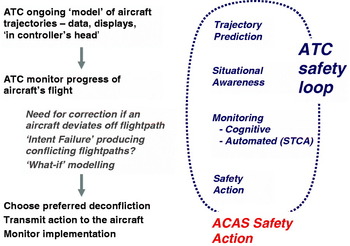
Part 1 sketches the historical origins of air traffic control (ATC) separation minima. It examines the safety thinking behind current minima and the issues involved in risk modelling. It tries to explain why the critical minima have largely remained unchanged for several decades – stasis. Figure 1 illustrates some key safety aspects of the existing concept. This human-centred operation places a variety of constraints on aircraft flightpaths. New concepts depend critically on accurate design and flight of ‘Four Dimensional Trajectories (4DT). These will be discussed in Part 2 (Brooker, Reference Brooker2011).
Key features of today's ATC safety concept.

2. SKETCH OF CURRENT ATC SEPARATION MINIMA ORIGINS
This section sketches some of the history of ATC separation minima in the UK. The focus is on Instrument Flight Rules (IFR) traffic subject to positive ATC. Other developed counties appear to have followed similar paths. The history is in part based on separation studies work done by the author in the 1970s. These included involved discussions with controllers who had been participants in the introduction of radar for civil purposes in the early 1950s. Later sections examine some of the issues in the quantitative modelling of ATC separation minima in the context of collision risks. These kinds of problems are certainly not unique to the UK. For example, FAA RADEC (2006) presents USA views on the kinds of research needed.
First, vertical separation is different from horizontal separation. The vertical minima were originally set by examining the then performance of barometric altimetry. Flight level differences of multiples of 1000 feet were easy to use. Controllers generally required that flightpaths for crossing aircraft are at fixed flight levels. Altimetry instrument performance was poorer at higher altitudes. This led to a breakpoint at 29,000 feet, with 1000 feet being used below that and 2000 feet above that. The locations of climbs and descents were generally very specific, mainly near airports. It is unusual to separate aircraft at minimum vertical separation while in climb/descent on an identical horizontal routeing. When aircraft climb or descend, the controller has to check several different flight levels, so this is a key element of his or her workload. Major studies into reductions of vertical separation minima were carried out from the 1980s onwards, e.g. Moek and Harrison (Reference Moek and Harrison1992) . They assessed improved altimetry using collision risk models. This led to a reduction in separation to 1000 feet. These models used largely assumed procedural ATC. Thus, they estimated the risk consequences of vertical navigation performance rather than the involvement of controllers.
Horizontal separation minima – termed ATC separation minima here – originated when controllers used primary radar. Historically, they are often termed radar minima. With primary radar, symbols (‘blips’) were roughly ellipses that varied in size with the distance from the radar head. This was called the beamwidth effect. Controllers had to ‘keep the blips apart’ to ensure safe separation – termed preventing resolution loss. Primary azimuth accuracy of targets was generally much worse than their range accuracy. With secondary processed radar, based on transponders carried by aircraft reporting the aircraft identity and height, the aircraft targets are shown by symbols. Thus, there is no indication of the distance from the radar head or which radar head being used. So what separation should the controllers now use between the symbols? The beamwidth – much narrower – is still there, but it is not made apparent to the controller.
In the 1970s, the UK decision was to set the minimum separation allowed between radar symbols so that the mid-air collision risk attributable to ATM was less than a target level of safety (TLS) (Brooker, Reference Brooker2004a). TLSs were determined in International Civil Aviation Organization (ICAO) work as ~10−8 fatal aircraft accidents per flying hour for mid-air collisions for en route flight in controlled airspace. TLSs were being used in major system changes, e.g. for North Atlantic flights and early work to reduce vertical separation. The main reason for the radar performance approach was that controllers wanted quantified assurance about equipment performance. Thus, the mid-air collision risk estimated by the chance of an aircraft pair, shown on the display as properly separated, in fact being at the same location in both azimuth and vertical dimensions. These risks are driven by the proportion of large errors in the statistical distribution of radar position errors.
The conclusions from the studies were that mid-air risk being less than TLS for radar inaccuracy implies:
• Range dependent radar separation minima
• 3 Nm in Terminal areas
• 5 Nm en route to limiting range of ~160/200 Nm
• 10 Nm beyond that
The 1970s derivations were a major step forward. But they were ‘static’ – they did not attempt to take properly into account how controllers use separation minima dynamically. For example, in reality, collisions do not happen instantly. The aircraft pair concerned must move from a safe configuration to a hazardous one. Radar-error collisions are thus caused by flawed flightpaths. These are dependent on both the initial positions of aircraft and their subsequent movements and velocities. It is therefore necessary first to identify hazardous (locally) correlated radar errors. The next step is to produce a robust model of the controller's decision processes (Brooker, Reference Brooker2004b).
3. QUALITATIVE THEORY FOR CURRENT ATC SEPARATION MINIMA
A good qualitative understanding of a system's safety properties is the starting point for a good quantitative model of those properties. While there is general agreement that the conceptual models used for vertical separation minima are appropriate, this is not the case for the ATC separation minima. This is important, because the sizes of these minima are key determinants of the economic operation of the system. If it were possible safely to reduce the minima significantly, there would be significant benefits arising from a system with nearer-direct routeing. This has been an issue of concern for many years. Magill (Reference Magill1998) presents some simulation results on potential savings. But the same ATC separation minima have been used for many decades. This stasis is in a context of extensive improvements in radar/flight data technology and displays. Moreover, highly effective conflict detection systems have been introduced, both on the ground and in the air (Brooker, Reference Brooker2008a gives some references).
This section therefore presents a simple qualitative descriptive theory for the use of current ATC separation minima. A framework for separation minima has to provide an understanding of the steps that link minima with mid-air collision risk. A good general background document is FAA/Eurocontrol (1998) . Probably the most perceptive comment is by Simpson (Reference Simpson1998) . In particular, Simpson tried to clarify their roles: “ATC separation criteria is usually an area of confused and non-rigorous analysis”. From a system point of view, separation minima are ‘formal rules’. They are the minimum distances that controllers should permit between aircraft. As explained earlier here, these minima were originally required because of inaccuracies in radar and altimetry data. In reality, ATC separation minima are largely ‘buffers’ to permit effective warnings and controller/pilot actions. (Radar accuracy and update rates cannot be the only factor in ATC separation minima. If radar data were 100% accurate and instantly available, the minima would surely not be set at zero distance.)
Separation minima exist because people make ATC decisions. Separation minima are not ‘guarantees’. They are constraints used by controllers. Quine (Reference Quine1987) sets out clearly the virtue of constraints as a freedom from decision. The advantage is that constraints limit the searches required. The controller does not have to carry out an assessment about the likelihood of a mid-air collision between pairs of aircraft. His or her task is to ensure that the separation minima are not breached. Thus, a decision about what one might do is replaced by an effective rule of thumb that establishes protection criteria between aircraft. Controllers are thus trained to achieve separation at greater than the minimum value rather than to avoid collisions. They operate with a specific goal rather than an open-ended goal.
Thus, separation minima deliver practical safety benefits because they help to reduce the variety of risk possibilities. Suppose there were no minima. In such a system, controllers would intervene to change flightpaths when they judged it necessary to prevent a potential serious conflict. Individual controllers would probably work with some minimum closest approach in mind. The closest separations would occur when they misjudged relative velocities or when there was insufficient time to instruct pilots to manoeuvre. There could be – infrequent – low separation values. These would often be in circumstances where the aircraft were close in position but in which their configuration/relative velocities would not be judged hazardous by independent observers. But these kinds of encounter would not be acceptable if a separation minimum were in operation. The general effect of the minimum is to move aircraft pairs which might have been at ‘near to zero’ separation to ‘greater than or near to the minimum’. From a risk viewpoint, the operational focus is on preventing undesirable deviations from a safe value rather than ensuring that encounters are not close to an unsafe separation.
But does the near elimination of some types of close encounter – many possibly not intrinsically risky – offer significant safety benefits? What indeed would be an unsafe separation? The starting point has to be what controllers actually do. There are a very large number of research papers on the cognitive and other tasks carried out by controllers. An often-quoted paper is Pawlak et al (Reference Pawlak, Brinton, Crouch and Lancaster1996) . They decompose air traffic control into a cycle of four main processes or tasks: evaluation, planning, implementation, monitoring. A mid-air collision could potentially occur if something goes seriously wrong with a combination of these processes.
Developed States gather evidence of close encounters between aircraft (e.g. UK Airproxes at http://www.airproxboard.org.uk/). The performances of navigation, communication, surveillance infrastructure systems or flight data processing are very seldom the major causal factor in a close encounter. These technological systems can fail, but very infrequently. There are normally well-established procedures in place to mitigate the risks involved and to recover until everything is functioning normally. A management failure to put safety mitigations in place to reduce the effects of partial equipment shutdowns can have tragic consequences. The key question is the intent of the flightpath as determined by controllers and pilots.
A failed intent implies a gross deviation from what would have been a reasonable intent. An aircraft with a reasonable intent follows a flightpath that is the consequence of reasonable controller/pilot decisions about safety. This process fails when people make misjudgements about priorities or assess something inaccurately. A controller could be distracted by an apparently much more serious issue elsewhere in his or her sector. The controller's plans could be flawed – an aircraft's flightpath is not where he or she should have intended it to go. There could be a sudden realisation by the controller that aircraft on tactically separated flightpaths are now in conflict, probably because he or she was distracted at the time when there ought to have been a tactical revision. A trainee controller might fail to keep to standard control procedures, but the controller mentor does not detect this failure. A pilot might decide to climb or descend because of some misunderstanding of a flight plan or of a controller's instructions.
How do these and other unusual occurrences affect the choice of separation minima? The simple answer is that the controller needs to have reservoirs of time for both detection and correction of gross failures. The focus on the time available is in the context of the speeds of the aircraft. This is perhaps 240 knots in a terminal area and 480 knots in en route airspace (hence 3 Nm and 5 Nm). Controllers need to be able to detect that an aircraft is following an unreasonable intent flightpath that is likely to generate collision risk. Thus, a separation minimum needs to be large enough so that it is highly probable that controllers will detect a large deviation from the planned flightpath well before any hazardous conflict.
The safety of today's developed ATC systems is in part assured by a variety of conflict aids. By extrapolating current radar tracks, these systems detect and alert possible close approaches of aircraft. This detection process is now aided by Short Term Conflict Alert (STCA). STCA alerts the controller/ supervisor to potentially conflicting flightpaths. (STCA is not intended to be a separation assurance tool. Such tools would use controller monitoring and automatic tools to determine if there will be a potential separation breach.) Most commercial flights carry an Airborne Collision Avoidance System (ACAS) as implemented by a Traffic Alert and Collision Avoidance System (currently TCAS II v7.0). ACAS is now an integral part of ATM safety performance. ACAS alerts the pilot to potentially conflicting aircraft. STCA has a much longer warning time than ACAS (respectively ~90 seconds and ~25 seconds before closest approach), and so prevents many possible ACAS alerts.
Brooker (Reference Brooker2005) notes that for UK incidents producing TCAS Resolution Alerts, the controller(s) are already aware of a potential conflict in about 90% of occasions. But also note that STCA cannot provide much help when there are sudden erroneous climbs/descents. Thus, controllers often try to focus on horizontal separation rather than vertical separation. As Averty (Reference Averty2005) reports: “ATCSs [controllers] seem not to have recourse to this [vertical] dimension as long as there is some evidence of lateral separation assessment.”
The effects of routine collision avoidance are important. ATM system design implicitly, and sometimes explicitly, assumes that passengers on aircraft want a much better ‘perceived safety experience’ than passengers in buses and coaches using the road network. Road journeys in congested city networks usually involve a high frequency of stops and decelerations. These are necessary to prevent possible very short-term conflicts with other road users. In contrast, the air passenger expects a smooth journey, without any obvious indication of possible conflicts – ‘ducking and weaving’ – with other aircraft. Thus, separation minima need to be large enough so that the frequency and magnitude of conflict preventing manoeuvres do not become a serious issue for the controller.
4. MODELLING COLLISION RISKS AND ATC SEPARATION MINIMA QUANTITATIVELY
What is the general nature of quantitative risk assessment as applied to socio-technical systems? These are systems whose performance relies on the interactions of people with technology. Quantitative risk assessments to predict post-system change safety levels generally require calculations using one or more Predictive Models. This means that some kind of predictive model, populated with appropriate data, is needed. The general task is to predict certain aspects of the various behaviours of this system. The key task is to estimate the changed system's safety performance. The main difficulty in modelling collision risks and ATC separation minima is determining what would be a ‘good enough’ model. The decision maker needs to be convinced that the model is a sufficiently good tool for safety-critical decisions. In reality, this decision-maker is an idealisation of the corporate bodies who approve system changes.
At an international level, there are different ways of determining separation minima. The key historical reference is ICAO (1998) . This identifies two safety assessment alternatives. In the first, there would be a relative comparison of proposed system risk with a reference. The proposed system is compared with an existing system that has already been judged acceptably safe. The reference system must be considered sufficiently similar to the proposed system. This method is most often used when there is a proposed technology change that does not materially affect the system's operational procedures/concepts. For example, there are several studies in the literature on surveillance systems using Automatic Dependent Surveillance-Broadcast as compared with secondary surveillance radar. This assumes that all operational factors except the surveillance technology are effectively unchanged. In the second alternative, there is an evaluation of the proposed system's risk against a threshold value – the TLS referred to earlier. This absolute method endeavours to determine an explicit relation between system characteristics and collision risk. The absolute approach has to be adopted when a radical change is planned that has not previously been tried elsewhere. The focus here is on the use of the absolute method, because a change in ATC separation minima could potentially alter the operation of the system in complex ways.
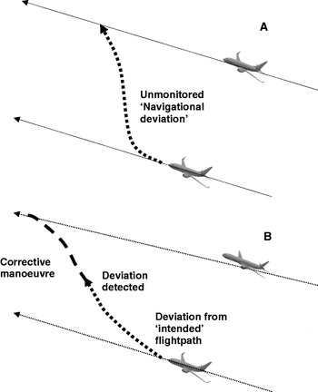
Several high quality research teams have tackled the problem of estimating the relationships between separation minima and collision risk. Most of the early work can be traced back to Reich (Reference Reich1966), which analysed procedurally separated aircraft without explicit ATC intervention. Important authors on separation minima aspects of collisions include Simpson (Reference Simpson1998), Reynolds and Hansman (Reference Reynolds, Hansman, Donohue and Zellweger2001), Shakarian and Haraldsdottir (Reference Shakarian and Haraldsdottir2001), and a European consortium (Mosquera-Benitez et al, Reference Mosquera-Benitez, Groskreutz and Fucke2009). These research studies have helped considerably in the understanding of the different safety processes involved. Modern work necessarily examines risks occurring through a succession of failures/errors. For example, if there is a deviation from the intended flightpath and then a corrective manoeuvre to prevent collision. Sometimes additional elements are explicitly included, e.g. ground-based conflict probes to assist the controller. The two types are illustrated in Figures 2A and 2B.
Changes in collision risk scenarios.

The separation minima and collision risk calculations vary in their details. Conceptually they must all include complex fault trees, but these can be constructed in different ways. They all endeavour to model the failures in the ATC processes. For a collision, there would have to be some kind(s) of gross problem(s) with flightpath intent, and then the detection of gross positional deviation or possible close approach, and then the consequent correction action would fail to address the problem. To predict long-term statistical risk, there has to be some statistical evidence-based simulation of traffic patterns and kinematics (i.e. the time entries and flightpath orientation of aircraft in the modelled airspace). It is necessary to model the key elements of data accuracy, human and equipment failure and error rates. ATC equipment performance, such as the latency of radar data, can be important. Aircraft/pilot characteristics, for example the time taken to receive instructions and to carry out manoeuvres, are very significant factors. Obviously, the size of the aircraft (i.e. their cross-section for collisions) is a key scaling factor.
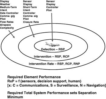
Collision risk calculation for ATC separation minima is inherently complex because of the different system elements that have to be given proper consideration. These include human performance, surveillance, communications, and navigation. Figure 3, adapted from Shakarian and Haraldsdottir (Reference Shakarian and Haraldsdottir2001), illustrates how ‘Required Total System Performance’ would set the value of the separation minimum. But it is not enough to conceive varieties of a functional dependence and list potentially significant factors. Those dependency factors need to be estimated quantitatively. The inherent problem is that there is a set of highly effective human/equipment safety defences in place. The task is to determine how frequently this complex combination will fail.
Separation minima and performance factors (adapted from Shakarian and Haraldsdottir (Reference Shakarian and Haraldsdottir2001) .

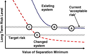
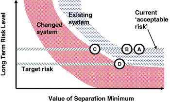
An ideal set of risk calculations would produce curves that might look like Figure 4. Brooker (Reference Brooker2008a) explains what kinds of ATM sub-systems can generate these kinds of results. Successful collision risk calculations justifying reductions in separation have generally focused on closed systems, e.g. navigation and altimetry. In these cases, gross errors leading to collision risk could be estimated by simply structured probabilistic modelling. The main requirements are changes to a single parameter, without complex human usage affecting that parameter, and a limited number of potential collision modes. Figure 4's curves show the risk/minimum relationship for two systems. One is the existing system and the other is a modified system with extra safety defences, and/or procedural ingredients and/or human/machine interface improvements, etc. The two illustrative curves represent estimated long-term risk for some specified amount of traffic. There is considerable debate about the nature of these risk curves. Should they include the safety improving effects of ground and aircraft-based collision warning and alert systems? Rationally, they should do so. If it is a mandatory requirement for safe system operation and is there to improve safety performance, then it is surely an integral part of the safety system. But there seems to be a degree of mental laziness about the topic at an institutional level (see Brooker, Reference Brooker2008a and related references there). For present purposes, it is assumed that the safety benefits of these systems for collision risk reduction are incorporated.
Perfect-world risk calculation versus safety target.

Point A on Figure 4 is a current separation minimum. It lies below the current ‘acceptable risk’, so the present system is judged to be safe – otherwise the regulator would insist on some additional risk mitigations. The curve is flat in this region. This implies that the value of the minimum is not a very critical parameter for collision risk, so the separation minimum could be reduced markedly to the value at point B. If the system were to be changed, the curve would move down markedly, so the new intersection point would be at point C. Thus, the existing system has a safety-cautious minimum, which could be reduced markedly without any system change. It could be further reduced markedly if the changed system were implemented. However, it might well be that policy makers would require the changed system to achieve a reduced risk level, e.g. because of the need to ensure safety for substantially increased traffic levels. Thus, if there were to be a reduced ‘target risk’ value, then this would produce the bottom line of the Figure, and hence the separation minimum could not be below point D.
The main problem with Figure 4 is that it portrays the curves as well defined. In reality, it is not possible to estimate precise curves for ATC separation minima calculations. A complex modelling framework to deal with this kind of open system problem needs to include all the necessary causal linkages, feedback loops and parameter estimates. The calculations producing the curves have to use estimates of the failure rates of the various ATM subsystems. These failure rates are usually very infrequent, so the probabilities are subject to sampling variations. In some cases, particularly when the failure mode is dependent on human performance, the failure rate may have to be an estimate based on broad knowledge of human error probabilities of a generic type. These kinds of human-related probabilities are seldom known with great precision, e.g. see Kirwan et al (Reference Kirwan, Kennedy, Taylor-Adams and Lambert1997), Kirwan et al (Reference Kirwan, Gibson and Hickling2008) . Nor is there agreement about what are the best models to assess human reliability, e.g. see Bell and Holroyd (Reference Bell and Holroyd2009) . Moreover, failure rates of successive safety defences may not be statistically independent. Thus, the conditional probability of a failure may depend on the existence of previous failures and the context in which the human agent is working, e.g. non-normal events, stress, etc. Risk estimation is difficult when there is the potential for a sequence of partially correlated failures/errors.
Collision risk models generally have several – sometimes many – free parameters that have to be estimated. If allowances are made for statistical variations in failure rates and the statistical relationships between subsystem failures, the simple curves in Figure 4 become the cloudier versions in Figure 5. Here the lines are replaced by some kind of statistical confidence band (but what kind and for what magnitude or error types?). The outcome, if the bands are viewed as no-go areas, is that both the B and C points move markedly to the right, i.e. there is much less scope for reducing the minimum. Again, if there were to be a reduced ‘target risk’ value, then this would produce the bottom line of the Figure, and hence the separation minimum could not be below point D.
Risk calculation versus safety target with model/parameter uncertainties.

5. MODELLING QUESTIONS
Is the estimation problem then solved by constructing something like Figure 5? The answer is no. A review of best practice in non-aviation safety work (Brooker, Reference Brooker2010) is clear that such predictions need validation. It is necessary to show that the predictive model possesses a satisfactory range of accuracy. This first requires a referent, which is codified information about the reality represented by the predictive model. Secondly, it requires some kind of means to enable extrapolation from the referent situation (e.g. the current system) to the changed system. An inadequate referent, a poor model structure, or a lack of appropriate data to calibrate the predictive model would mean that the prediction could not be validated. By chance, it might happen to be a good prediction, but an honest analyst could not express confidence about its quality. Even the most complex mathematics cannot compensate for flimsy validation processes.
Ironically, many of ATM's risk modelling problems stem from the fact that aviation is a very safe mode of transport. Accidents, especially mid-air collisions involving commercial aircraft, happen comparatively infrequently. They are now usually the product of a complex sequence of failed system defences. This means that ATM risk estimates are inherently uncertain. Modelling uncertainties covers both random variations and lack of knowledge about the ATM system. The first is termed aleatory uncertainty and the second is termed epistemic uncertainty. Aleatory derives from the Latin for gambler and epistemic is from the Greek word for knowledge. Aleatory uncertainty means that the events or phenomena being modelled are characterized as occurring in a ‘random’, or ‘stochastic’, manner, so probabilistic models are adopted to describe their occurrences. Helton and Burmaster (Reference Helton and Burmaster1996) offer the useful distinction:
“… aleatory uncertainty, which arises because the system under study can behave in many different ways and is thus a property of the system, and epistemic uncertainty, which arises from a lack of knowledge about the system and is thus a property of the analysts performing the study.”
In practice, it is not always easy to distinguish clearly between the two categories. Sometimes a division is made based on convenience linked to features of the problem being studied as well as to the current state of knowledge/ignorance (e.g. Kiureghian and Ditlevsen, Reference Kiureghian and Ditlevsen2009). A very interesting paper by Morgan et al (Reference Morgan, Dowlatabadi, Henrion, Keith, Lempert, McBride, Small and Wilbanks2009) offers a different approach, focusing on the nature of modelling. This splits uncertainty into two parts: ‘uncertainty about the value of empirical quantities’ and ‘uncertainty about model functional form’.
Brooker (Reference Brooker2010) discusses lessons from environmental, nuclear and defence modelling. They are relevant to ATM safety because those disciplines have also had to confront the limitations of modelling the rates of rare and potentially catastrophic events. The most formally developed approach to these issues is probably in the nuclear field. Some key explanatory references are Parry (Reference Parry1996), Caruso et al (Reference Caruso1999) and NUREG (2009) . The last of these is an official publication by the USA's Nuclear Regulatory Commission. Parry (Reference Parry1996) provided a simple description of the different kinds of epistemic uncertainty:
“[epistemic] Uncertainty was categorized into three types; parameter uncertainty, modelling uncertainty, and completeness uncertainty … it can be argued that the distinction made in the PRA Procedures Guide between parameter uncertainty and modelling uncertainty is fundamentally artificial, it is certainly useful from a practical point of view. Parameter uncertainty can be thought of as addressing uncertainty in the quantification of a model with a specified functional form, whereas model uncertainty can be thought of as addressing the uncertainty in the appropriateness of the structure or mathematical form of the model. Completeness uncertainty is a special category of model uncertainty that is associated with the degree to which the model addresses all the phenomena associated with the system being modeled. Whether it is possible, or even makes sense, to try to capture completeness uncertainty formally, however, is open to question, and will not be addressed here.”
A variety of examples of each of the uncertainty categories are given in Caruso et al (Reference Caruso1999) .
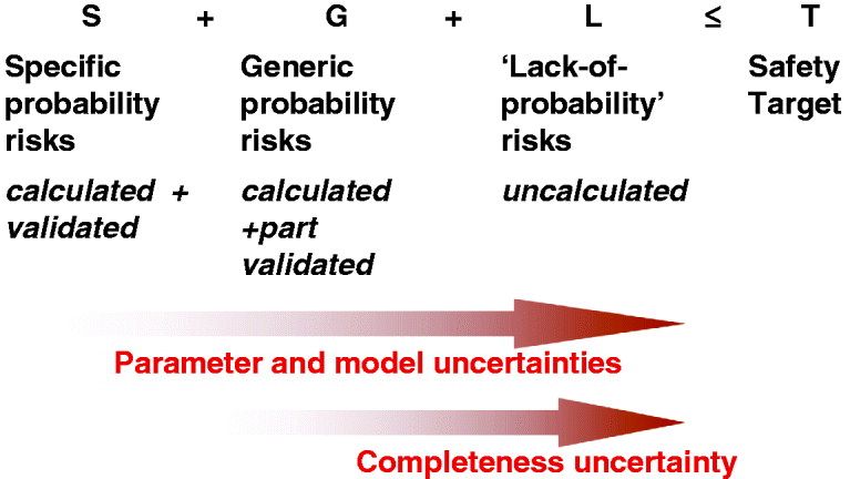
In the present context, the effects of these uncertainties can be illustrated by Figure 6. This divides accident risks into three categories, which are summed for comparison with the appropriate safety target. From earlier comments, there is an obvious issue about what allowance should be made for the degree of statistical confidence of risk estimates. The first category, S – specific probability risks – can be calculated using a good predictive model. A consensus of analysts would judge them to be derived by reasonable processes, i.e. they are validated. An example is a model based on Figure 2A. For the current system, these kinds of risks would be extremely small, simply because the additional safety defences in place would imply that a single factor accident is highly improbable.
Accident risk categories versus safety target.
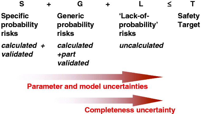
The second category in Figure 6, G – generic probability risks – are again calculated. But in this case either or both the accident model and the data to populate such models are known in only broad terms, i.e. would be part validated. Models based on failures in the process shown in Figure 2B would be of this type. For example, the probabilities of corrective action being successful might be a large extrapolation from actual data, or based on approximate human error probabilities. They might even include models for organisational factors (e.g. Mohaghegh et al, Reference Mohaghegh, Kazemi and Mosleh2009).
The effects of system parameter shifts are important in the G category. This covers the need for modelling of risk-related parameters where there are feedbacks involved. One example is the change in closest approach distances if the minimum is changed. A reduction in the minimum from 5 Nm to (say) 4 Nm will change the statistical distribution of actual closest approach distances, e.g. 7 Nm in practice might become 6 Nm. To model the effects of a change, good estimates would be needed for the shift in actual statistical distributions, which might well be different between individual controllers. Another example is the STCA triggering parameters. A reduction in the minimum would require a change to these parameters. Otherwise, for example, the number of false and/or unnecessary alerts would tend to increase, with consequent effects on controllers trust in the alerting system.
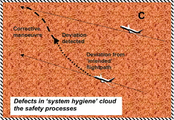
The third category on Figure 6, L – ‘lack-of-probability’ risks – would not have been calculated (and obviously not validated). It would be the collective contribution of very rare risks from multi-causal factor accidents. These expose latent weaknesses in a variety of safety defences. Each accident may well appear to be a unique, almost unrepeatable event. Key factors are professional lapses and mismanagement. A metaphor would be poor cleanliness and contaminated drinking water when treating a diseased patient. The system hygiene is impaired, which then reduces ATM system effectiveness by ‘clouding’ the safety processes – i.e. Figure 2 becomes Figure 7. Examples of risk outcomes in this third category would be the mid-air collisions at Überlingen (e.g. Brooker, Reference Brooker2008b) and in Brazil (Lacagnina, Reference Lacagnina2009; National Transportation Safety Board, 2008). At the time of writing, these two tragedies were in fact the only two mid-air collisions involving commercial jets during the last decade. This system hygiene category would also apply to some collisions on the ground, e.g. at Milan Linate in 2001. SRC (2005) is an extremely relevant analysis – in particular Chapter 7. System hygiene issues now appear to be the most frequent kind of mid-air collision – the dominant risk. This is because of the improvements in equipment, procedures, training, safety alerting systems, etc. These have markedly reduced what would have been the risk contributions for simple one, two or three causal factor accidents.
Cloudy collision risk scenarios.

Note that accidents in the third category are not unimaginable, e.g. see de Jong (Reference de Jong2004) (which aims to construct tests for system resilience). They are, however, unexpected. This is in the strict sense that it seems virtually impossible to construct a validated accurate prediction of the statistical expectation of such a collective. If there is some kind of jumble of multiple causal factors in a poor system hygiene context, then a separation minimum reduction would tend to increase risks.
Possibility or conjecture are not the same as actual knowledge. Thus, for present purposes, the problem is that of completeness. Models use knowledge about failure modes and their frequencies to estimate risk. If these models are incomplete then the risk estimate could be in error – particularly so given that the risk estimates in this context are of very rare events. The point is nicely made by Shakarian and Haraldsdottir (Reference Shakarian and Haraldsdottir2001) :
“However, to actually propose reductions in en-route route minima to values of 4 or even 3 [Nm] will require a complete evaluation of the effects of rare-normal and non-normal conditions and configurations assessed in various complex traffic flow structures.”
A facet of this ‘rare event’ problem is illustrated in Figure 8, inter alia picking up the point made earlier about aircraft speeds en route and in terminal areas. Supposing that the normal ATC system fails to provide separation, this shows the time to collision for aircraft at a specific relative velocity from a starting point of a variety of separation minimum values. Thus, suppose two aircraft are 3 Nm apart and approaching with a relative velocity of 600 knots. They collide in 18 seconds. If (say) 20 seconds were judged the minimum time required for an ACAS device to warn the pilot, then it would not be acceptable for this configuration. A 20-second line is shown in the Figure. The smaller the separation minimum the more likely it is that a lower relative velocity would result in a breach of the 20 seconds or other time criterion. (Compare with TCAS II alert parameters, e.g. see page 20 of FAA (2000) .)
Time to collision as a function of distance apart and relative speed.

Nor is risk modelling the only consideration. Non-safety consequences would include the changes in operational performance that might result from a minimum change. The obvious example is on the capacity of the system. Authors such as Chaboud et al (Reference Chaboud, Hunter, Hustache, Mahlich and Tullett2000) and Loft et al (Reference Loft, Sanderson, Neal and Mooij2007) discuss how sector capacity depends on a controller's workload components. Some of these are simply related to the passage of the aircraft through the sector, but others are focused on preventing collisions. For example, the controller checks visually on the screen and uses flight data information to investigate if aircraft might come into conflict. If the minimum is reduced then, all other things being equal, the controller might increase the frequency of such checks. This would tend to increase the total workload required for a given amount of traffic, and hence reduce the amount of traffic that could be handled safely, ie reduce the sector capacity. This adaptive behaviour would match the controller's perception (sic) of the system risks. Studies of this ‘Risk-adaptation’ have a long history, e.g. see Koornstra (Reference Koornstra2009) .
6. CONCLUSIONS
There is considerable institutional interest in reducing separation minima to achieve economic benefits. The main conclusion from this brief sketch is that it is intrinsically difficult to change ATC separation minima. The problems are not with researchers or analysts. The calibre of people working in this area is high, and their work has produced useful models and subtle insights. The same methodological themes are repeated but definitive conclusions are not generated. The difficulty is in estimating risks with high confidence. Can the effects of changes be understood quantitatively ‘beyond reasonable doubt’?
Risk calculations can be done with confidence if the leading risk contributions are from measurable single probabilities, and these can include simple types of human errors. But ATM safety has improved considerably over recent decades. There have been improvements in equipment, procedures, training, etc. Safety-alerting systems have been introduced. Together, these changes have markedly reduced what would have been the risk contributions for simple one, two or three causal factor accidents. The leading risks now derive from combinations of human error probabilities that are at best measurable in general terms. These estimates are subject to large modelling uncertainties. Recent accidents have in fact been the product of multi-causal factors, including safety hygiene factors. These include poor management and operator training. This suggests that future accidents will generally be rare, almost unique events, whose frequency it is near impossible to estimate with any precision.
The outputs of quantitative safety modelling do not add up to a sufficient condition to persuade ATM decision makers of future acceptable safety performance for reduced ATC separation minima for the current operational concept.