2.1. Contact analysis between a single drive wheel and the curved surface of the pipeline

The various postures of the robot within the pipeline must be analyzed in response to different command actions, considering the robot’s posture [Reference Qi, Zhang, Chen and Ye22]. As the robot’s rigid body is fully supported by four wheels, the study of robot posture ultimately involves examining the contact relationship between the wheels and the cylindrical surface of the pipeline.

A comprehensive study of the robot’s postural scenarios was approached by examining the contact between a single wheel and the pipeline’s cylindrical surface. Generally, such problems were analyzed and described by assessing the contact point and the velocity at the wheel center. For a more rigorous analysis, the following assumptions were established:

• • Both the wheel and the pipeline are perfectly rigid bodies, with no deformation occurring upon contact.

• • Pure rolling motion exists between the wheel and the pipeline, with no slippage.

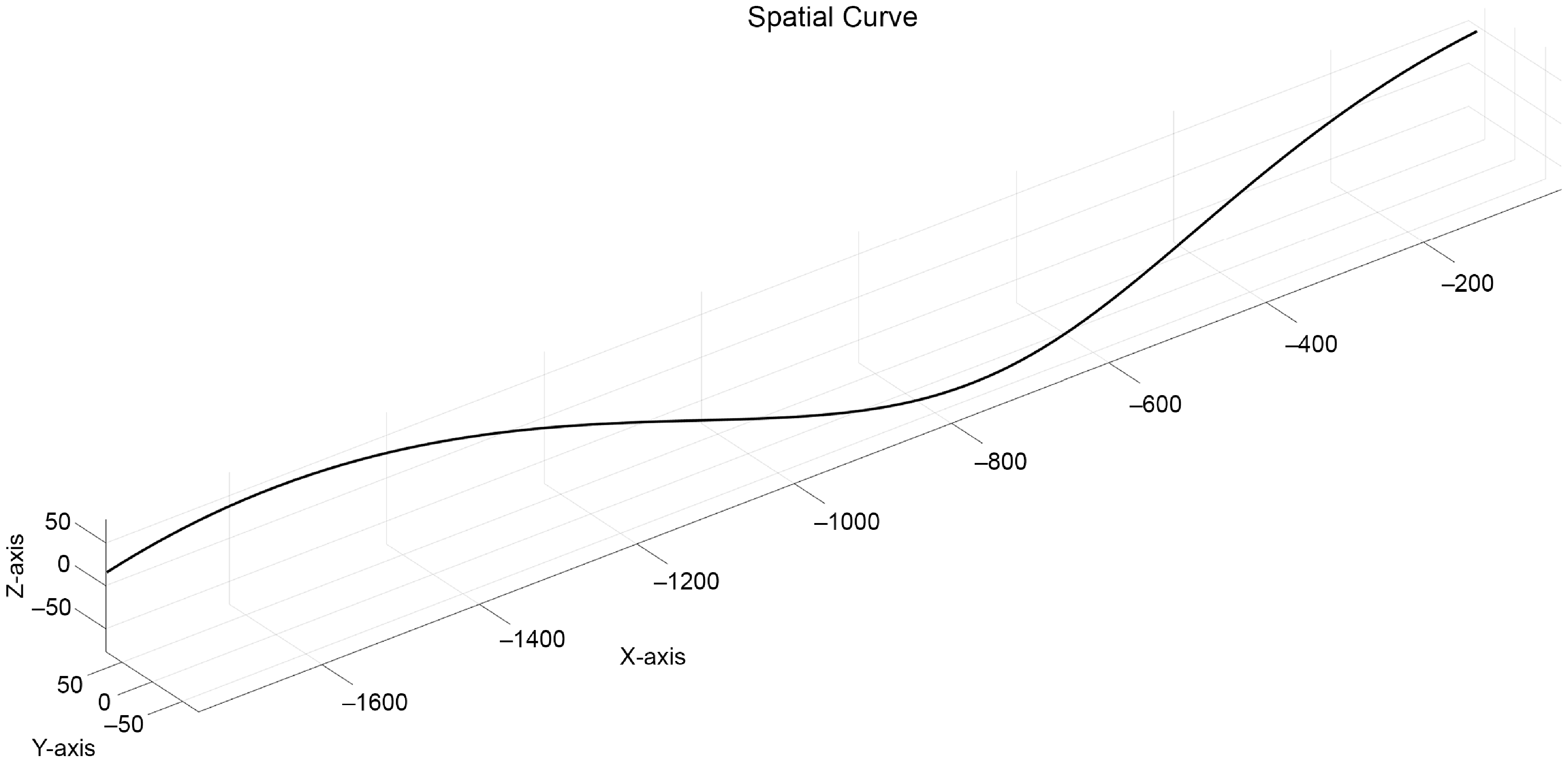
Based on these assumptions, the inference is that there is a point of contact between the wheel and the cylindrical surface of the pipeline. As the wheel rolls forward, the contact point on the wheel manifests as a spatial curve passing through the contact point on the wheel rim, while on the cylindrical surface, it appears as a typical spatial curve segment. This relationship is abstracted into a three-dimensional mathematical model, for which an absolute coordinate system is established, as shown in the Figure 1.

Figure 1.

The spatial curve of the wheel center.

Referring to the three-dimensional diagram in the Figure 2, the largest surface depicted above represents the inner cylindrical surface of the pipeline, while the ellipse denotes the wheel’s contact rim line at an arbitrary angle. By connecting the wheel center $O_{0}$ to the contact point $O_{1}$ at a given moment $t$ , the segment $O_{0}O_{1}$ represents the effective contact rim radius of the wheel, and the magnitude of this segment is $r$ . The normal M was drawn through the contact point $O_{1}$ , which is a generatrix of the cylindrical surface inside the pipeline, and the radius $O_{0}O_{1}$ was used for this purpose. The cross-section of the cylindrical surface passing through the contact point $O_{1}$ and the normal $P$ of the cross-section intersect with the axis $Q$ of the cylindrical surface and $O_{2}$ . The segment $O_{1}O_{2}$ was characterized by a size of $R$ , which represents the semi-diameter of the cylindrical surface within the pipeline at a certain moment. α is the angle between the normal $M$ and the normal $N$ , and the angle is $\beta$ between the radius $O_{0}O_{1}$ and the normal $P$ .

Figure 2.

Single wheel rolling model inside the pipeline.

When the control input is defined by the rotational speed of the drive motor $\omega _{0}$ , the wheel achieves an angular velocity ${\unicode[Arial]{x03C9}}$ through the transmission mechanism. Regardless of how the robot’s steering causes $\alpha$ to change, the collection of contact point positions on the cylindrical surface forms a spatial curve. Consequently, the cumulative contact point positions outline the spatial curve traversed by the wheel, which is spatial trajectory $p(t)$ .

(1) \begin{equation} \begin{array}{c} p\left(t\right)=\left[\begin{array}{c} -\omega \cdot t\cdot r\cdot \cos \alpha \\ R\cdot \cos\!\left(-\omega \cdot t\cdot r\cdot \sin \alpha /R\right)\\ R\cdot \sin\!\left(-\omega \cdot t\cdot r\cdot \sin \alpha /R\right) \end{array}\right]^{T} \end{array} \end{equation}

The $\textit{Frenet}$ active coordinate system was established at the contact point $O_{1}$ by utilizing the tangent vector, the principal normal, and the binormal as the coordinate axes.

In the active coordinate frame, the coordinates of the wheel center were given by $(0,\,r\cos \beta ,\,r\sin \beta )$ . To obtain the coordinates of the wheel center in the absolute coordinate system, a coordinate transformation matrix $\textit{Hartenberg}-\textit{Denavit}$ was introduced, as follows: $D^{(ij)}=\left[\begin{array}{ccc} A^{(ij)} & \vdots & d_{ij}^{(i)}\\ \cdots & \vdots & \cdots \\ 0 & \vdots & 1 \end{array}\right]$ . The ellipsis in this matrix represents the omission of the element “ $0$ ”.

Among them:

(2) \begin{align} A^{\left(ij\right)}=e^{\left(i\right)}\cdot e^{\left(j\right)T}=\left[\begin{array}{c@{\quad}c@{\quad}c} \tau & n & b \end{array}\right]^{T}\cdot e^{\left(j\right)T} \end{align}

(3) \begin{align} d_{ij}^{\left(i\right)}=\left[\begin{array}{c} -\omega \cdot t\cdot r\cdot \cos \alpha \\ R\cdot \cos\!\left(\frac{-\omega \cdot t\cdot r\cdot \sin \alpha }{R}\right)\\[5pt] R\cdot \sin\!\left(\frac{-\omega \cdot t\cdot r\cdot \sin \alpha }{R}\right) \end{array}\right] \end{align}

Then, Eqs. (2) and (3) were substituted into the coordinate transformation matrix equation to obtain Eq. (4).

Based on the data measurements obtained from the SolidWorks 3D model, the following equations were derived: $r=100\text{ mm},R=150\text{ mm}$ . When $\alpha$ was set to $\pi /6$ , $\beta$ to $\pi /6$ , and $\omega$ to 1(rad/s), the following spatial curve was obtained through MATLAB simulation as shown in Figure 3.

(4) \begin{align} \left[\begin{array}{c} x \\ y \\ z \\ 1 \end{array}\right] = D^{(ij)}\cdot \left[\begin{array}{c} 0\\ r{\cos}\;\beta\\ r{\sin}\;\beta\\ 1 \end{array}\right]\left[\begin{array}{c} -r\cdot \sin\;\beta \sin\;\alpha - \omega{tr}\cdot \cos\;\alpha\\-r\cdot \cos\;\beta \cos\!(\frac{\omega{tr\sin\;\alpha}}{R}) + r\cdot \sin\;\beta \cos\;\alpha \sin\!(\frac{\omega{tr\sin\;\alpha}}{R})+R \cdot \cos\!(\frac{\omega{tr\sin\;\alpha}}{R})\\[4pt] r\cdot \cos\;\beta \sin\!(\frac{\omega{tr\sin\;\alpha}}{R}) + r\cdot \sin\;\beta \cos\;\alpha \cos\!(\frac{\omega{tr\sin\;\alpha}}{R})-R \cdot \sin\!(\frac{\omega{tr\sin\;\alpha}}{R})\\1\end{array} \right] \end{align}

It can be observed that the position of the wheel center is closely related to time and can be controlled and determined with ω, α, and β given.

2.2. Analysis of the posture of pipeline robot moving forward normally in a straight line

Considering the characteristics of municipal pipelines, most of the robot’s operational time was spent on straight lines, which represented its standard working conditions.

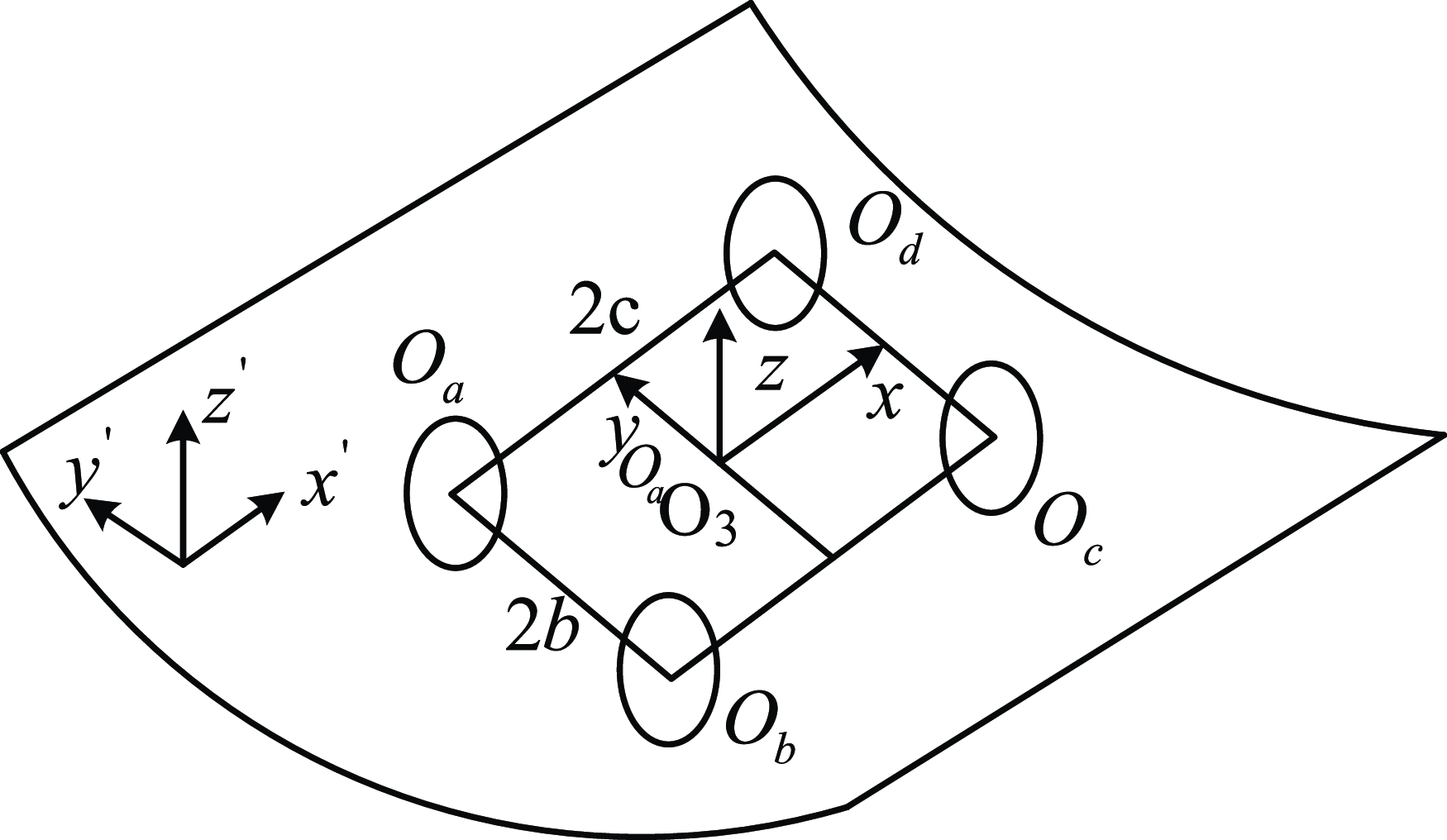
The position and orientation of the robot within the pipeline underwent certain changes. To mathematically study these changes and potential patterns, a specific reference point on the robot’s rigid body was selected. The absolute coordinates and the associated Euler angles of the point were used to represent the two main states of the robot. Prior to this analysis, similar to the earlier analysis of a single wheel, the model was first abstracted into a planar mathematical form. For clarity, the robot’s movements are decomposed into translation and rotation: the robot’s relocation from an initial position to a target position can be considered as a spatial displacement combined with a rotation around a designated point on its body.

In the Figure 3, to further analyze displacement and rotation, Cartesian coordinates and Euler angles were utilized. The centers of the robot’s four wheels were denoted as $O_{a}$ , $O_{b}$ , $O_{c}$ , and $O_{d}$ , forming a fixed spatial rectangle with length $2c$ and width $2b$ . The origin $O_{3}$ was set at the center of this rectangle, with the x-axis passing through the midpoint of the line segment $O_{c}O_{d}$ , the y-axis through the midpoint of $O_{a}O_{d}$ , and the z-axis perpendicular to the plane of the rectangle, creating a moving coordinate frame. From the perspective of Euler angles, the robot’s orientation was defined by three angles of rotation $\delta$ , $\theta$ , and $\mu$ , which represent the rotations about the x-axes, y-axes, and z-axes, respectively.

Figure 3.

Four wheel rolling model inside the pipeline.

By converting the point coordinates in the above moving coordinates into absolute coordinates (the absolute coordinate system construction method is consistent with Section 2.1, omitted here), the coordinates of the wheel center in the absolute coordinate system are obtained.

According to the definition of Euler angle and the transformation matrix equation, the Euler angle formula $R(\delta ,\theta ,\mu )$ can be obtained.

(5) \begin{equation} \begin{array}{c} R\left(\delta ,\theta ,\mu \right)=\left[\begin{array}{ccc} \mathit{\cos }\;\mathit{\delta }\cos\theta &\quad \mathit{\cos }\;\mathit{\delta }\mathit{\sin }\;\mathit{\theta }\sin\mu -\mathit{\sin }\;\mathit{\delta }\cos\mu &\quad \mathit{\cos }\;\mathit{\delta }\mathit{\sin }\;\mathit{\theta }\cos\mu +\mathit{\sin }\;\mathit{\delta }\sin\mu \\ \mathit{\sin }\;\mathit{\delta }\,\cos\theta &\quad \mathit{\sin }\;\mathit{\delta }\mathit{\sin }\;\mathit{\theta }\sin\mu +\mathit{\cos }\;\mathit{\delta }\cos\mu &\quad \mathit{\sin }\;\mathit{\delta }\mathit{\sin }\;\mathit{\theta }\cos\mu -\mathit{\cos }\;\mathit{\delta }\sin\mu \\ \begin{array}{c} -\!\sin\theta \\ 0 \end{array} &\quad \begin{array}{c} \mathit{\cos }\;\mathit{\theta }\sin\mu \\ 0 \end{array} &\quad \begin{array}{c} \mathit{\cos }\;\mathit{\theta }\cos\mu \\ 0 \end{array} \end{array}\begin{array}{c} 0\\ 0\\ \begin{array}{c} 0\\ 1 \end{array} \end{array}\right] \end{array} \end{equation}

Assuming that the coordinates $(x,y,z)$ , represent the point coordinates in an absolute coordinate system, the coordinates $(x_{0},y_{0},z_{0})$ denote the origin of the moving coordinate system in the absolute coordinate framework. The coordinates of any point on the rigid body of the robot in the moving coordinate system are represented as $x\mathrm{''},y\mathrm{''},z\mathrm{''}$ . So, the Eq. (6) can be obtained through the coordinate axis conversion formula.

(6) \begin{equation} \begin{array}{c} \left[\begin{array}{c} x\\ y\\ \begin{array}{c} z\\ 1 \end{array} \end{array}\right]=D^{\left(ij\right)}\left[\begin{array}{c} x\mathrm{''}\\ y\mathrm{''}\\ \begin{array}{c} z\mathrm{''}\\ 1 \end{array} \end{array}\right] \end{array} \end{equation}

Among them, $D_{ij}=\left[\begin{array}{c@{\quad}c} R(\delta ,\theta ,\mu ) & d_{ij}\\ 0 & 1 \end{array}\right]$ , $d_{ij}=\left[\begin{array}{c} x_{0}\\ y_{0}\\ z_{0} \end{array}\right]$ .

The coordinates of the centers of the robot’s four wheels were denoted as $K$ in the motion coordinate system, while in the absolute coordinate system, they were denoted as $J$

(7) \begin{align}&\qquad\qquad J=\left[\begin{array}{c@{\quad}c} \begin{array}{c@{\quad}c} x_{a} & x_{b}\\ y_{a} & y_{b}\\ z_{a} & z_{b} \end{array} & \begin{array}{c@{\quad}c} x_{c} & x_{d}\\ y_{c} & y_{d}\\ z_{c} & z_{d} \end{array} \end{array}\right] \end{align}

(8) \begin{align}& K=\left[\begin{array}{c@{\quad}c} \begin{array}{c@{\quad}c} x_{a}^{\mathrm{''}} & x_{b}^{\mathrm{''}}\\ y_{a}^{\mathrm{''}} & y_{b}^{\mathrm{''}}\\ z_{a}^{\mathrm{''}} & z_{b}^{\mathrm{''}} \end{array} & \begin{array}{c@{\quad}c} x_{c}^{\mathrm{''}} & x_{d}^{\mathrm{''}}\\ y_{c}^{\mathrm{''}} & y_{d}^{\mathrm{''}}\\ z_{c}^{\mathrm{''}} & z_{d}^{\mathrm{''}} \end{array} \end{array}\right]=\left[\begin{array}{c@{\quad}c} \begin{array}{c@{\quad}c} -c & -c\\ b & -b\\ 0 & 0 \end{array} & \begin{array}{c@{\quad}c} c & c\\ -b & b\\ 0 & 0 \end{array} \end{array}\right] \end{align}

Substitute Eqs. (7) and (8) into Eq. (6) to obtain Eq. (9).

(9) \begin{equation} \begin{array}{c} L=\left[\begin{array}{c} J\\ 1 \end{array}\right]=D^{\left(ij\right)}\left[\begin{array}{c} K\\ 1 \end{array}\right]=\left[\begin{array}{cc} \begin{array}{cc} x_{a} & x_{b}\\ y_{a} & y_{b}\\ \begin{array}{c} z_{a}\\ 1 \end{array} & \begin{array}{c} z_{b}\\ 1 \end{array} \end{array} & \begin{array}{cc} x_{c} & x_{d}\\ y_{c} & y_{d}\\ \begin{array}{c} z_{c}\\ 1 \end{array} & \begin{array}{c} z_{d}\\ 1 \end{array} \end{array} \end{array}\right] \end{array} \end{equation}

Finally, four wheel’s center coordinates were obtained.

(10) \begin{equation} \begin{array}{c} \left[\begin{array}{c} x_{a}\\ y_{a}\\ z_{a} \end{array}\right]=\left[\begin{array}{c} -c\cos\;\delta \cos\;\theta +b\sin\;\mu \!\left(\cos\;\delta \sin\;\theta -\sin\;\delta \right)+x_{0}\\ y_{0}-c\sin\;\delta \cos\;\theta +b\!\left(\sin\;\delta \sin\;\theta \sin\;\mu +\cos\;\delta \cos\;\mu \right)\\ c\sin\;\theta +b\cos\;\theta \sin\;\mu +z_{0} \end{array}\right] \end{array} \end{equation}

(11) \begin{equation} \begin{array}{c} \left[\begin{array}{c} x_{b}\\ y_{b}\\ z_{b} \end{array}\right]=\left[\begin{array}{c} x_{0}-c\cdot \mathit{\cos }\;\mathit{\delta }\cos\theta -b\!\left(\mathit{\cos }\;\mathit{\delta }\mathit{\sin }\;\mathit{\theta }\sin\mu -\mathit{\sin }\;\mathit{\delta }\sin\mu \right)\\ y_{0}-c\cdot \mathit{\sin }\;\mathit{\delta }\cos\theta -b\!\left(\mathit{\sin }\;\mathit{\delta }\mathit{\sin }\;\mathit{\theta }\sin\mu +\mathit{\cos }\;\mathit{\delta }\cos\mu \right)\\ c\cdot \sin\theta -b\cdot \mathit{\cos }\;\mathit{\theta }\sin\mu +z_{0} \end{array}\right] \end{array} \end{equation}

(12) \begin{equation} \begin{array}{c} \left[\begin{array}{c} x_{c}\\ y_{c}\\ z_{c} \end{array}\right]=\left[\begin{array}{c} c\cdot \mathit{\cos }\;\mathit{\delta }\cos\theta -b\!\left(\mathit{\cos }\;\mathit{\delta }\mathit{\sin }\;\mathit{\theta }\sin\mu -\mathit{\sin }\;\mathit{\delta }\sin\mu \right)+x_{0}\\ c\cdot \mathit{\sin }\;\mathit{\delta }\cos\theta -b\!\left(\mathit{\sin }\;\mathit{\delta }\mathit{\sin }\;\mathit{\theta }\sin\mu +\mathit{\cos }\;\mathit{\delta }\cos\mu \right)+y_{0}\\ -c\cdot \sin\theta -b\cdot \mathit{\cos }\;\mathit{\theta }\sin\mu +z_{0} \end{array}\right] \end{array} \end{equation}

(13) \begin{equation} \begin{array}{c} \left[\begin{array}{c} x_{d}\\ y_{d}\\ z_{d} \end{array}\right]=\left[\begin{array}{c} c\cdot \mathit{\cos }\;\mathit{\delta }\cos\theta -b\!\left(\mathit{\cos }\;\mathit{\delta }\mathit{\sin }\;\mathit{\theta }\sin\mu -\mathit{\sin }\;\mathit{\delta }\sin\mu \right)+x_{0}\\ c\cdot \mathit{\sin }\;\mathit{\delta }\cos\theta -b\!\left(\mathit{\sin }\;\mathit{\delta }\mathit{\sin }\;\mathit{\theta }\sin\mu +\mathit{\cos }\;\mathit{\delta }\cos\mu \right)+y_{0}\\ -c\cdot \sin\theta -b\cdot \mathit{\cos }\;\mathit{\theta }\sin\mu +z_{0} \end{array}\right] \end{array} \end{equation}

In addition, parameter equations for four wheels contacting the outer circle were introduced. Equation (14) was the outer circle expression matrix.

(14) \begin{equation} \begin{array}{c} H=\left[\begin{array}{cc} \begin{array}{cc} \cos t_{1}-c &\quad \cos t_{2}-c\\ b &\quad -b\\ \sin t_{1} &\quad \sin t_{2} \end{array} &\quad \begin{array}{cc} c+\cos t_{3} &\quad c+\cos t_{4}\\ -b &\quad b\\ \sin t_{3} &\quad \sin t_{4} \end{array} \end{array}\right] \end{array} \end{equation}

Based on specific geometric relationships, it is observed that the tangent vector of each wheel’s contact point on the rim curve is perpendicular to the normal vector of the tangent plane at the cylindrical contact surface. The coordinates $(x_{o},y_{o},z_{o})$ of each contact point lie on the cylindrical surface of the pipeline, satisfying the equation $y_{o}^{2}+z_{o}^{2}=R^{2}$ . When all four wheels meet this condition, a system of eight equations can be formulated. Solving for the unknowns $t_{1},t_{2},t_{3},t_{4}$ in the matrix $H$ required four of these equations, and four remaining equations were left.

Based on the above analysis, there was still a need to solve for six unknowns $x_{o},y_{o},z_{o},\delta ,\theta ,\mu$ , but four equations remained unsolved. When $\textit{Positioning}=\{x,y,z,\delta ,\theta ,\mu \}$ was selected to represent the specific posture of the robot at work, since $x_{o}$ was independent, one of the other five factors affecting the posture could accurately express the robot’s posture.

Therefore, during straight-line motion under normal conditions, the pipeline robot theoretically experiences only translational displacement along one direction. Assuming the detected displacement was $x=x_{m}$ , the positioning was obtained as $\textit{Positioning}=\{x_{m},0,0,0,0,0\}$ . Clearly, determining the exact magnitude and direction of this single displacement is a critical factor for the robot’s effective and reliable operation under these conditions.

2.3. Analysis of nonLinear action posture of pipeline robots

When the robot’s path deviated from a straight line, such as during turns or when traversing the side of a cylindrical pipeline, typically only three of the four wheels maintained direct contact with the pipe wall. Utilizing the results from the previous discussion, this scenario was denoted as $\textit{Positioning}=\{x,y,z,\delta ,\theta ,\mu \}$ , and six constraint equations were formulated. By eliminating three parameters, five unknowns remained to be solved simultaneously, two of which were known quantities.

Given the difficulty in accurately surveying the robot’s precise coordinate values after it enters the pipeline, it is essential to equip the robot with a gyroscope to obtain real-time values for angles $\delta ,\theta$ and $\mu$ .

3.1. Analysis of the dimensions of robot bending bodies

Assuming that the envelope dimensions of the robot were $\mathit{L}\mathrm{*}h\mathrm{*}b$ , the robot is encapsulated within a rectangular prism of corresponding dimensions. The robot’s ability to pass through a pipeline is not solely dependent on its maximum cross-sectional dimensions $(h\mathrm{*}b)$ but also on the curvature of the pipeline. If the curvature at a bend is smaller and the pipeline is straighter, the robot will find it easier to navigate. Among common pipeline configurations, a 90-degree bend presents the greatest challenge for passage. Therefore, the following discussion is focused on the study of 90-degree pipelines.

For the robot to traverse pipes of specified dimensions and curvature, the dimensions $L$ , $h$ , and $b$ of the robot had to meet certain criteria. Assuming the diameter of the pipeline was $D$ , the radius of the pipeline was $r$ , and the curvature radius was $R$ . Additionally, the diagonal of the robot’s cross-sectional envelope dimensions was set as $d$ . The geometric constraints for passing through a 90-degree pipeline [Reference An, Lee, Oh, Moon and Ryew23] are then given by:

(15) \begin{equation} \begin{array}{c} \begin{cases} \left(R+r\right)\cos45^{\circ}-\left(R-r\right)\lt d\lt D\\ L=2\sqrt{\left(R+r\right)^{2}-\left(R-r+d\right)} \end{cases} \end{array} \end{equation}

In robots, $d=\sqrt{(h^{2}+b^{2})^{2}}$ , so Eq. (15) yields Eq. (16).

(16) \begin{equation} \begin{array}{c} L=2\sqrt{\left(R+r\right)^{2}-\left(R-r+\sqrt{\left(h^{2}+b^{2}\right)^{2}}\right)} \end{array} \end{equation}

The aforementioned equations were implemented in the MATLAB, where the model parameters were set as $D=2r=300\text{ mm}$ , $R=400\text{ mm}$ . The relationship between $L$ and $h$ was examined, with the parameter $b$ being determined based on the design specifications of the robot’s body, specifically $b=200\text{ mm}$ . Conversely, when the relationship between $L$ and $b$ was investigated, the parameter $h$ was established as $h=200\,\mathrm{mm}$ according to the design specifications. This analysis yielded the following graphs: In Figure 4, the relationship between $L$ and h was displayed, as well as the relationship between $L$ and $b$ . The following conclusions can be drawn from the observations made in the above figure:

Figure 4.

L-h or b relationship curve.

• • Both $b$ and $h$ were found to have an identical influence on $L$ , where $L$ was observed to exhibit a curvilinear decline as either $b$ or $h$ increased.

• • The three-dimensional image depicting the influence of $b$ and $h$ on $L$ exhibited a symmetrical bowl-like shape. It was observed that $L$ was highly sensitive to parameter variations when $b$ or $h$ was less than 100 mm. However, when $b$ or $h$ exceeded 200 mm, the change in $L$ became gradual. In Figure 5, the color gradient tending toward red indicated larger values of $L$ , approaching the limit, which implied a reduced capability of the four-wheeled robot to navigate through curved pipes.

Figure 5.

Three dimensional trend image of the influence of b and h on L.

3.2. Analysis of robot cornering speed

When the pipeline robot navigates a bend, it is necessary not only to satisfy the above geometric constraints but also to account for the dynamic constraints during the movement process. Specifically, if the robot could not rotate around the curvature center when making a turn, the velocities $v_{i}(i=1,2,3,4)$ of each wheel’s contact point with the inner surface of the cylindrical pipeline must be proportional to the respective radii of the curvature $R_{i}(i=1,2,3,4)$ at those contact points, such that $v_{1}\colon v_{2}\colon v_{3}\colon v_{4}=R_{1}\colon R_{2}\colon R_{3}\colon R_{4}$ .

The turning maneuver of the robot involves two distinct phases: the transition phase and the rotation phase. To investigate the relationship between the velocities at the four wheels’ contact points and the radii of curvature during these two phases, the following mathematical model in Figure 6 was conducted.

Figure 6.

The robot passes through a curved coordinate system.

Starting from the transition stage, the coordinate matrix of the contact points of the four wheels in the $O_{2}$ coordinate system can be obtained by using the dimension relationship shown in Figure 6(a).

(17) \begin{equation} \begin{array}{c} \left[\begin{array}{c} W_{1}^{2}\\ W_{2}^{2}\\ \begin{array}{c} W_{3}^{2}\\ W_{4}^{2} \end{array} \end{array}\right]^{T}=\left[\begin{array}{cccc} 0 & 0 & L & L\\ {r\sin}\;\gamma & -{r\sin}\;\gamma & {r\sin}\;\gamma & -{r\sin}\;\gamma \\ -{r\cos}\;\gamma & -{r\cos}\;\gamma & -{r\cos}\;\gamma & -{r\cos}\;\gamma \end{array}\right] \end{array} \end{equation}

\begin{equation*} \left[\begin{array}{c} W_{1}^{0}\\ W_{2}^{0}\\ \begin{array}{c} W_{3}^{0}\\ W_{4}^{0} \end{array} \end{array}\right]^{T}=\overrightarrow{O_{0}O_{2}}+\frac{1}{2}{R}{}\left[\begin{array}{c} W_{1}^{2}\\ W_{2}^{2}\\ \begin{array}{c} W_{3}^{2}\\ W_{4}^{2} \end{array} \end{array}\right]^{T}= \end{equation*}

(18) \begin{equation} \begin{array}{c} \left[\begin{array}{c@{\quad}c@{\quad}c@{\quad}c} R\alpha -L & R\alpha -L & R\alpha -L+L\cos \theta & R\alpha -L+L\cos \theta \\+r\sin \gamma \sin \theta & -r\sin \gamma \sin \theta & +r\sin \gamma \sin \theta & -r\sin \gamma \sin \theta \\ R+r\sin \gamma \cos \theta & R-r\sin \gamma \cos \theta & R-L\sin \theta +r\sin \gamma \cos \theta & R-L\sin \theta -r\sin \gamma \cos \theta \\ -r\cos \gamma & -{r\cos}\;\gamma & -{r\cos}\;\gamma & -{r\cos}\;\gamma \end{array}\right] \end{array} \end{equation}

After the coordinate transformation in the transition stage, Eq. (17) 1 becomes Eq. (18).

$W_{i}^{2}$ represented the coordinates of the four wheels in the $O_{2}$ coordinate system, while $W_{i}^{0}$ denoted the coordinates of the four wheels in the $O_{0}$ coordinate system. The rotation matrix $X$ corresponds to the transformation from the $O_{1}$ coordinate system to the $O_{2}$ coordinate system, where $\mathrm{X}=\left[\begin{array}{c@{\quad}c@{\quad}c} \cos \theta & \sin \theta & 0\\ -\sin \theta & \cos \theta & 0\\ 0 & 0 & 1 \end{array}\right]$ , $\overrightarrow{O_{0}O_{2}}=[\begin{array}{ccc} R\alpha -L & R & 0 \end{array}]^{T}$ , $\sin \gamma =2/3$ , $\theta$ is the angle of rotation during the transformation from the $O_{1}$ coordinate system to the $O_{2}$ coordinate system, with $\theta =\sin ^{-1} \frac{R\left(1-\cos \alpha \right)}{L}$ . The angle $\alpha$ was considered, which represents the rotation of the body around the curvature center of the bending tube during the transition phase. The value of $\alpha$ during this phase is small, therefore, based on Taylor’s formula, the following approximations are employed: $\sin \alpha \approx \alpha$ , $\cos \alpha \approx 1$ .

Differentiating Eq. (18) yields the velocity matrix Eqs. (19) and (20) for each contact point.

(19) \begin{equation} \begin{array}{c} {V}=\frac{{dW}_{{i}}^{0}}{{dt}}=\left[\begin{array}{c@{\quad}c@{\quad}c@{\quad}c} {v}_{1{x}} & {v}_{2{x}} & {v}_{3{x}} & {v}_{4{x}}\\ {v}_{1{y}} & {v}_{2{y}} & {v}_{3{y}} & {v}_{4{y}}\\ {v}_{1{z}} & {v}_{2{z}} & {v}_{3{z}} & {v}_{4{z}} \end{array}\right] \end{array} \end{equation}

(20) \begin{equation} \begin{array}{c} \left[\begin{array}{c@{\quad}c} v_{1x} & v_{2x}\\ v_{1y} & v_{2y}\\ v_{1z} & v_{2z} \end{array}\right]=\left[\begin{array}{cc} R\alpha \mathrm{'}+r\alpha \mathrm{'}\sin \gamma \sin \alpha & R\alpha \mathrm{'}-r\alpha \mathrm{'}\sin \gamma \sin \alpha \\ \frac{-rR\alpha \mathrm{'}\sin \gamma \sin \theta \sin \alpha }{\sqrt{L^{2}-R^{2}\left(1-\cos \alpha \right)^{2}}} & \frac{rR\alpha \mathrm{'}\sin \gamma \sin \theta \sin \alpha }{\sqrt{L^{2}-R^{2}\left(1-\cos \alpha \right)^{2}}}\\ 0 & 0 \end{array}\right] \end{array} \end{equation}

After the transition phase, the robot entered a relatively simple rotational phase. During this period, the wheels on both sides of the robot had identical contact point trajectories and velocities. Assuming the robot rotates by an angle $\beta$ around the curvature center, the rotational velocity matrix $V\mathrm{'}$ can be obtained based on the aforementioned method.

Indices $I$ and $O$ represent the inner side and outer side, respectively, in proximity to the curvature center. $W_{IO}^{0}$ denotes the coordinate matrix of the contact points of the inner and outer wheels in the $O_{0}$ coordinate system.

Substituting $\alpha _{1}=2\sin ^{-1} \left(\frac{L}{2R}\right)$ into Eq. (22), the relationship between the speed magnitude and time can be obtained, Combined with writing $v_{i}=\sqrt{v_{ix}^{2}+v_{iy}^{2}+v_{iz}^{2}}$ .

(21) \begin{equation} \begin{array}{c} \left[\begin{array}{c@{\quad}c} v_{3x} & v_{4x}\\ v_{3y} & v_{4y}\\ v_{3z} & v_{4z} \end{array}\right]=\left[\begin{array}{cc} R\alpha \mathrm{'}+r\alpha \mathrm{'}\sin \gamma \sin \alpha +\frac{LR\alpha \mathrm{'}\sin \alpha \sin \theta }{\sqrt{L^{2}-R^{2}\left(1-\cos \alpha \right)^{2}}} & R\alpha \mathrm{'}+r\alpha \mathrm{'}\sin \gamma \sin \alpha -\frac{LR\alpha \mathrm{'}\sin \alpha \sin \theta }{\sqrt{L^{2}-R^{2}\left(1-\cos \alpha \right)^{2}}}\\ -R\alpha \mathrm{'}\sin \alpha -\frac{rR\alpha \mathrm{'}\sin \gamma \sin \theta \sin \alpha }{\sqrt{L^{2}-R^{2}\left(1-\cos \alpha \right)^{2}}} & \frac{rR\alpha \mathrm{'}\sin \gamma \sin \theta \sin \alpha }{\sqrt{L^{2}-R^{2}\left(1-\cos \alpha \right)^{2}}}-R\alpha \mathrm{'}\sin \alpha \\ 0 & 0 \end{array}\right] \end{array} \end{equation}

(22) \begin{align} V\mathrm{'}=\frac{dW_{IO}^{0}}{dt}=\left[\begin{array}{c@{\quad}c} v_{Ix} & v_{Ox}\\ v_{Iy} & v_{Oy}\\ v_{Iz} & v_{Oz} \end{array}\right]=\left[\begin{array}{cc} R\beta \mathrm{'}\cos \beta +r\beta \mathrm{'}\sin \gamma \cos\!\left(\beta +\frac{\alpha _{1}}{2}\right) & R\beta \mathrm{'}\cos \beta -r\beta \mathrm{'}\sin \gamma \cos\!\left(\beta +\frac{\alpha _{1}}{2}\right)\\ -R\beta \mathrm{'}\sin \beta -r\beta \mathrm{'}\sin \gamma \sin\!\left(\beta +\frac{\alpha _{1}}{2}\right) & r\beta \mathrm{'}\sin \gamma \sin\!\left(\beta +\frac{\alpha _{1}}{2}\right)-R\beta \mathrm{'}\sin \beta \\ 0 & 0 \end{array}\right]\notag \\ \end{align}

Angles $\alpha$ and $\beta$ represent the rotation around the curvature center during two distinct phases. For the sake of analysis, it is assumed that the robot undergoes uniform angular were changed during both phases, so that $\alpha =k_{1}t_{1}, \beta =k_{2}t_{2}$ . Consequently, $\alpha \mathrm{'}=k_{1}$ and $\beta \mathrm{'}=k_{2}$ .

• • During the transition phase in the Figure 7, the velocity trends of the four wheels’ contact points are generally similar, characterized by three notable speed “peaks” at 13, 49, and 75 s, where the velocities are significantly higher than those at adjacent time intervals. The rapid and substantial changes in velocity near these three moments can lead to considerable energy dissipation in the robot. Therefore, it is advisable to avoid these speed “peaks” by adjusting the values of $k_{1}$ and $k_{2}$ to make a low-speed, smooth transition strategy during this phase.

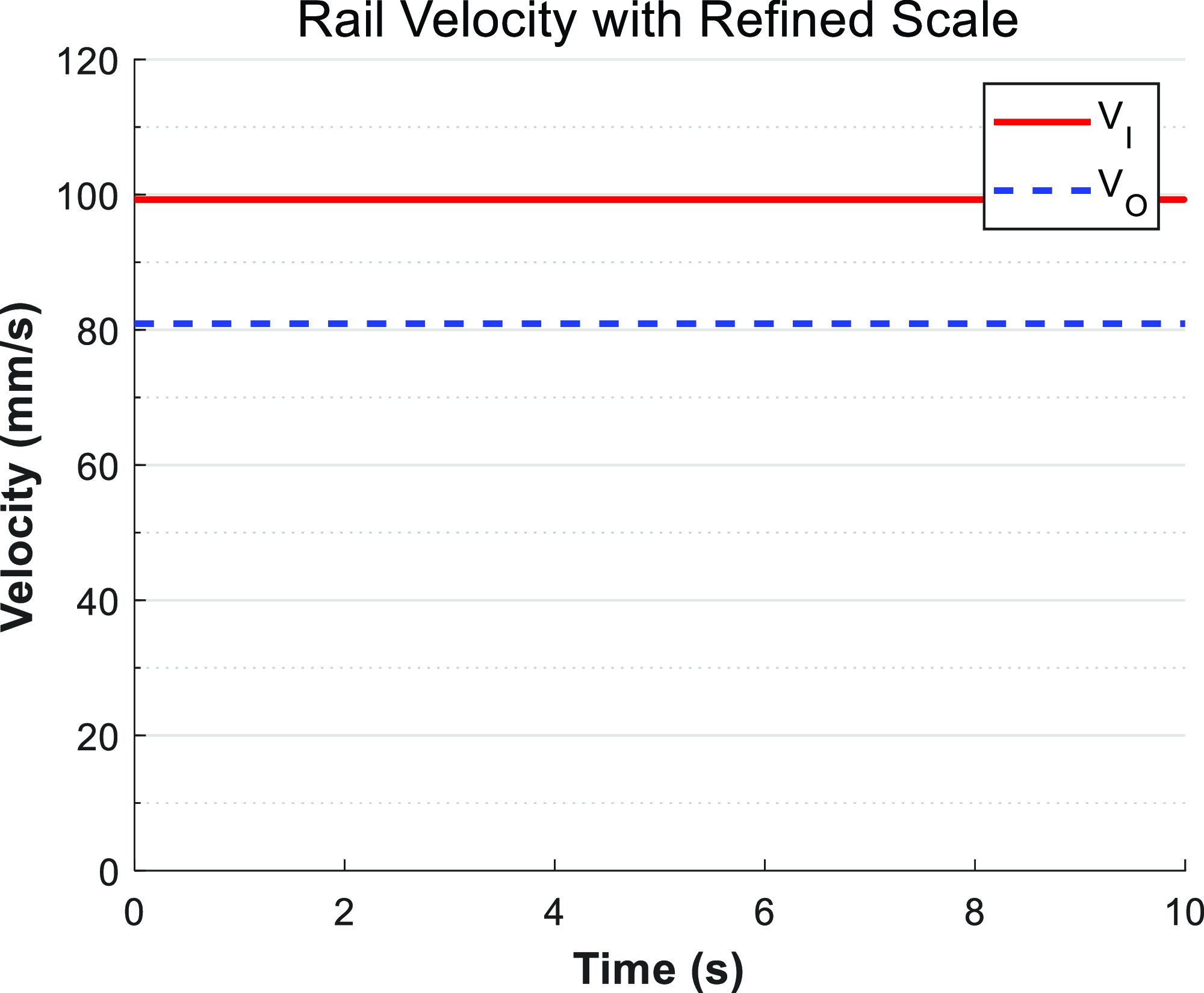
• • In the rotation phase in the Figure 8, the robot’s velocity remains relatively constant, with the speed being proportional to the radii of curvature at the corresponding contact points. This results in stable and smooth operation of the robot.

• • It is evident that the ability of the robot to stabilize during the transition phase is crucial for ensuring successful and smooth navigation through the bend.

Figure 7.

The speed of the transition phase versus time curve.

Figure 8.

The curve of the velocity of the inner and outer sides during the rotation phase with respect to time.

4.1. Mathematical analysis of robot’s field of view direction control

It could be understood from the previous discussion that the flexibility of wheeled pipeline robots was somewhat lacking, and typical pipeline robots were generally equipped with only two-degree-of-freedom (DOF) vision components. This limitation became particularly evident when the robot was unable to move along the pipeline axis, preventing the use of the robot’s rigid body to increase the DOFs of the vision component. As a result, the robot’s field of view was significantly reduced. To address this limitation, a three-degree-of-freedom vision component was designed in this study to be mounted on the robot’s rigid body.

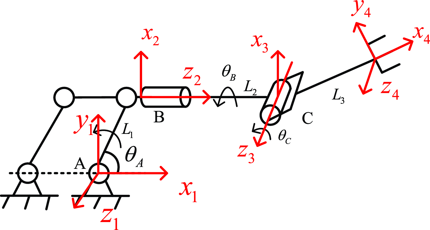
In comparison to pipeline robots with fewer degrees of freedom in their camera components, three-degree-of-freedom pipeline robots demonstrate higher efficiency and greater convenience. To control the variables, the camera component is isolated and abstracted into a schematic diagram of the mechanism’s motion, as shown in the Figure 9, with the corresponding coordinate system established as depicted. The axes $z_{1}$ , $z_{3}$ , and $z_{4}$ are all perpendicular to the plane of the paper.

In the Figure 9, points $A,B$ , and $C$ represent the connection rotational pairs of the three components. $L_{1}, L_{2},$ and $L_{3}$ denote the lengths of the linkages abstracted from the individual components. The section preceding point B and the section following point B were separated and modeled independently. For the section before point B, the homogeneous transformation matrix at the end, i.e., the position of point B, was calculated. For the section after point B, the SDH (Standard Denavit-Hartenberg) modeling approach was employed [Reference Wang and Lien24, Reference Shrey, Patil, Pawar, Lokhande, Dandage and Ghorpade25], and the position transformation matrix of the end effector, ${2}^{3}{T}{}$ , was derived.

Figure 9.

SDH coordinate system for three degree of freedom camera components.

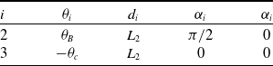
$i$ was used to denote the joint index, $\theta _{i+1}$ represented the angle required for the coordinate system to rotate around the $z_{i}$ axis until the $x_{i+1}$ axis was parallel to the $x_{i}$ axis. $d_{i+1}$ was the distance necessary for the coordinate system to translate along the $z_{i}$ axis until the $x_{i+1}$ and $x_{i}$ axes were collinear. $\alpha _{i+1}$ was the angle required for the coordinate system to rotate around the $x_{i}$ axis until the $z_{i+1}$ axis was parallel to the $z_{i}$ axis, and $a_{i+1}$ was the distance required for the coordinate system to move along the $x_{i}$ axis until the two coordinates overlap [Reference Tung, Tinh, Thao and Minh26, Reference Alebooyeh and Urbanic27]. The corresponding $D-H$ table is established as Table 1.

$\theta _{A},\theta _{B}$ and $\frac{\pi }{2}-\theta _{C}$ are the angles where three joints rotate. Equations (25) and (26) were obtained, based on Eq. (23). According to the point A, the rotation matrix of the camera component after undergoing a series of actions is $X_{a}$ . Correspondingly, its spatial position vector is $X_{b}$ .

(23) \begin{align} &{}_{i+1}^{i}{T}{}=Rot\!\left(X,\theta _{i+1}\right)\textit{Trans}\!\left(0,0,d_{i+1}\right)Rot\!\left(Z,\alpha _{i+1}\right)\textit{Trans}\!\left(a_{i+1},0,0\right)\\ &=\left[\begin{array}{c@{\quad}c@{\quad}c} \begin{array}{c} \cos\theta _{i+1}\\ \sin\theta _{i+1}\\ \begin{array}{c} 0\\ 0 \end{array} \end{array} & \begin{array}{c} -\sin\theta _{i+1}\cos\alpha _{i+1}\\ \cos\theta _{i+1}\cos\alpha _{i+1}\\ \begin{array}{c} \sin\alpha _{i+1}\\ 0 \end{array} \end{array} & \begin{array}{c@{\quad}c} \begin{array}{c} \sin\theta _{i+1}\sin\alpha _{i+1}\\ -\cos\theta _{i+1}\sin\alpha _{i+1}\\ \begin{array}{c} \cos\alpha _{i+1}\\ 0 \end{array} \end{array} & \begin{array}{c} a_{i+1}\cos\theta _{i+1}\\ -a_{i+1}\sin\theta _{i+1}\\ \begin{array}{c} d_{i+1}\\ 1 \end{array} \end{array} \end{array} \end{array}\right] \end{align}

(24) \begin{align} _{0}^{1}{T}{}=\left[\begin{array}{c@{\quad}c@{\quad}c} \begin{array}{c} 1\\ 0\\ \begin{array}{c} 0\\ 0 \end{array} \end{array} & \begin{array}{c} 0\\ 1\\ \begin{array}{c} 0\\ 0 \end{array} \end{array} & \begin{array}{c@{\quad}c} \begin{array}{c} 0\\ 0\\ \begin{array}{c} 1\\ 0 \end{array} \end{array} & \begin{array}{c} L_{1}\cos \theta _{A}\\ L_{1}\sin \theta _{A}\\ \begin{array}{c} 0\\ 1 \end{array} \end{array} \end{array} \end{array}\right] \end{align}

(25) \begin{align} X_{a}=\left[\begin{array}{c@{\quad}c@{\quad}c} \begin{array}{c} \cos \theta _{B}\cos \theta _{C}\\ \sin \theta _{B}\cos \theta _{C}\\ -\sin \theta _{C} \end{array} & \begin{array}{c} \cos \theta _{B}\sin \theta _{C}\\ \sin \theta _{B}\sin \theta _{C}\\ \cos \theta _{C} \end{array} & \begin{array}{c} \sin \theta _{B}\\ -\cos \theta _{B}\\ 0 \end{array} \end{array}\right] \end{align}

(26) \begin{align} X_{b}=\left[\begin{array}{c} L_{1}\cos \theta _{A}\cos \theta _{B}\cos \theta _{C}+L_{1}\sin \theta _{A}\cos \theta _{B}\sin \theta _{C}+L_{3}\sin \theta _{B}\\ L_{1}\cos \theta _{A}\sin \theta _{B}\cos \theta _{C}+L_{1}\sin \theta _{A}\sin \theta _{B}\sin \theta _{C}-L_{3}\cos \theta _{B}\\ L_{2}-L_{1}\cos \theta _{A}\sin \theta _{C}+L_{1}\sin \theta _{A} \end{array}\right] \end{align}

Upon examining the two results above, it was observed that the position and orientation of the robot’s camera component were solely determined by the rotation angles of the three rotational pairs when the lengths of the linkages were established. Therefore, to accurately observe a specific location within the pipeline, it is essential to input the designated joint angles. This information was then relayed to the motors, which corresponded to different rotational speeds at specific time intervals $t_{A},t_{B}$ and $t_{C}$ . To ensure precision, it is necessary to employ motors equipped with feedback mechanisms, such as Hall effect encoders.

Table I.

D-H parameter table.

4.2. Simulation and modeling of three degree of freedom field of the view for camera components

By modeling and measuring data, using the Solidworks $3D$ software, the lengths $L_{i}$ of the three connecting rods were obtained. Subsequently, the data was input into the MATLAB, utilizing the SDH method for the forward kinematics of the robot. The range of motion for the three joints was set with a limit of $\begin{cases} \theta _{A}\in (\pi /6,\pi /2)\\ \theta _{B}\in (-\!\pi /2,\pi /2)\\ \theta _{C}\in (-\!\pi /2,\pi /2) \end{cases}\!\!\!\!\!\!$ , resulting in a three-dimensional scatter plot depicting the random distribution of the end-effector camera in space.

The randomly distributed points in Figure 10 represent the set of distribution points when the camera’s focal length is set to zero. It is evident that the robot’s field of the view forms a segment of an arc-shaped surface. This configuration occurred because the camera’s focal length was not taken into account in the aforementioned calculations and simulations, and it is the camera’s focal length that determines the distance at which targets can be observed. To effectively observe the details within the pipeline, the robot’s camera component must be equipped with a lens that has a specific focal length. Assuming the focal length of the camera was $x$ , it is sufficient to observe the interior walls of the pipeline. The maximum effective area that the camera component could scan was a portion of the cylindrical surface attached to the interior of the pipeline, when the robot remained in a fixed position. This cylindrical surface area is referred to as the maximum effective field of the view of the pipeline robot within the pipeline.

Figure 10.

Random position of end camera in 3D space with joint constraints.

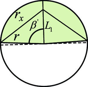
The center $O_{3}$ in Figure 11(a) is the end of the third joint of the camera component, and $r_{x}$ is the combination of the camera line of sight and the third link, which includes a focal segment of $x$ was denoted as $r_{x}$ , that is, $r_{x}=L_{3}+x$ . Assuming that $O_{0}$ is the center point of the pipeline cross-section, and $O_{0}$ is also the starting point A of the camera component.

The Eq. (27) can be obtained from Figure 11(a) and (b), Eq. (28) can be obtained by combining all the equations in Eq. (27).

(27) \begin{equation} \begin{array}{c} \begin{cases} \cos \beta =\left[r^{2}+{L_{1}}^{2}-\left(L_{3}+x\right)^{2}\right]/\left(2rL_{1}\right)\\ l_{ab}=r\times 2\beta \\ \cos \theta _{L}=\frac{r}{r_{x}+L_{1}}\\ L=M+N=\left(L_{1}+r_{x}\right)\sin \theta _{L} \end{cases} \end{array} \end{equation}

(28) \begin{equation} \begin{array}{c} \begin{cases} l_{ab}=2r\cos ^{-1} \left(\frac{r^{2}+{L_{1}}^{2}-\left(L_{3}+x\right)^{2}}{2rL_{1}}\right)\\ L=\left(L_{3}+x+L_{1}\right)\sin \!\left(\cos ^{-1} \frac{r}{L_{3}+x+L_{1}}\right) \end{cases} \end{array} \end{equation}

Figure 11.

Cross section of the viewing angle range.

So, the maximum effective field of the view of the robot is $S_{\max}$ .

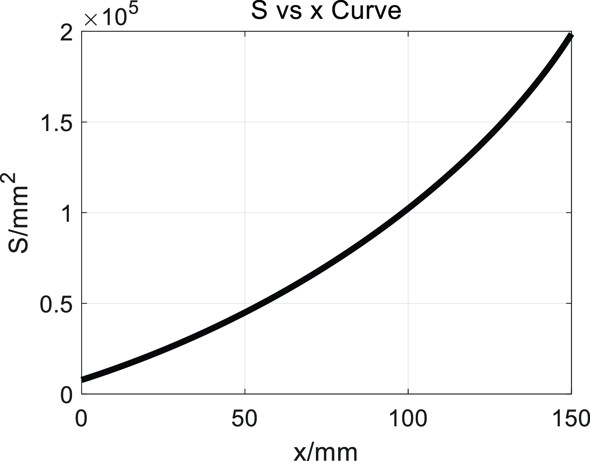
Substituting $L_{3}=74.5\text{ mm}$ , $\;L_{1}=90\text{ mm}$ and $r=150\,{\rm mm}$ into Eq. (29), and simulating the results using the MATLAB, the relationship curve between the maximum effective field of view $S_{\max}$ and the focal length $x$ can be obtained.

(29) \begin{equation} \begin{array}{c} S_{\max}=L\times l_{ab}=2r\left(L_{3}+x+L_{1}\right)\sin \!\left(\cos ^{-1} \frac{r}{L_{3}+x+L_{1}}\right)\cos ^{-1} \left[\frac{r^{2}+{L_{1}}^{2}-\left(L_{3}+x\right)^{2}}{2rL_{1}}\right] \end{array} \end{equation}

From the observations presented in the Figure 12, the following conclusions can be drawn:

• • When $x=100\,{\rm mm}$ , the maximum effective field of the view of the pipeline robot is $S_{\max}=1\times 10^{5}\,{\rm mm}^{2}$ .The maximum range was $2\beta \mathrm{'}$ that $S_{\max}$ could cover on a plane perpendicular to the axis, and $2\beta \mathrm{'}=$ 2 $\cos\!\left(\frac{r^{2}+{L_{1}}^{2}-{r_{x}}^{2}}{2rL_{1}}\right)\approx 179.4^{\circ}$ . Therefore, when $x=100\,{\rm mm}$ , the upper half of the pipeline interior was visible to the robot, as shown in Figure 13.

• • The maximum effective field of the view $S_{\max}$ of the robot increases as the focal length $x$ continues to grow.

• • The rate of the increase of the curve also rises with the increase of $x$ ; that is to say, under the given constraints, as ${\unicode[Arial]{x0394}} x$ becomes larger, each increment in $x$ results in a greater increase in the field of the view. Therefore, when designing the visual component of the pipeline robot, the maximum value of $x$ should be selected while satisfying its spatial geometric constraints.

Figure 12.

The curve of $S$ about $x$ .

Figure 13.

Maximum cross-sectional field of view under specified focal segment.

4.3. Kinematic simulation of a three degree of freedom camera component

The homogeneous transformation matrix, including the rotation matrix and position matrix, for the forward kinematics of a three-degree-of-freedom vision-based module was derived and simulated. The time-varying curves of each joint angle and angular velocity were obtained, along with the time-varying curve of the linear velocity of the end effector. These curves were plotted, as shown in Figure 14, to observe their dynamic characteristics.

Figure 14.

The angle, angular velocity of each joint, and linear velocity of the end effector over time curve.

Since the lengths of the linkages for the three assembled joints are fixed, the position of the terminal camera is determined by the angles rotated by the three joints, which are represented as $(\theta _{A},\theta _{B},\theta _{C})$ to indicate the joint states. From the observations in the figures above, the following conclusions can be drawn:

• • In Figure 14(a), it was observed that the robot’s camera component started from a random initial state $(\pi /6,-\pi /3,-\pi /2)$ , and after the changes described in Section 4.1, reached a randomly designated state $(\pi /3,\pi /3,0)$ , and the inverse transformation was performed to return to the initial state.

• • Correspondingly, the speed of each joint rotating to the target position exhibited an approximately linear variation, indicating that the fluctuation in joint acceleration was minimal and that each joint of the module operated stably.

• • As shown in Figure 14(c), the velocities of the end effector in three directions were different at the beginning but all became zero at $t=5\,{\rm s}$ . This represented a certain path planning for the three joints to reach the designated positions. Along this path, the velocities underwent both increase and decrease, and the velocity variation curves were smooth without sharp points, indicating that the results derived from Eqs. (25) and (26) were relatively accurate. Based on this, the control principle used to drive the three-degree-of-freedom vision-based module was feasible.