1. Introduction
Liquid films and shallow flows are often examined in the limit where the Reynolds number
 $Re$
and the slope
 ${\it\varepsilon}$
of the free surface are both small, in which case the problem can be simplified using the lubrication approximation (LA). In particular, the LA was applied to hydraulic jumps (bores) developing in flows down an inclined substrate when the upstream depth
 $h_{-}$
exceeds the downstream depth
 $h_{+}$
(Benney Reference Benney1966; Mei Reference Mei1966; Homsy Reference Homsy1974; Lin Reference Lin1974; Bertozzi & Brenner Reference Bertozzi and Brenner1997; Bertozzi et al.
Reference Bertozzi, Münch, Fanton and Cazabat1998, Reference Bertozzi, Münch, Shearer and Zumbrun2001; Bertozzi & Shearer Reference Bertozzi and Shearer2000; Chang & Demekhin Reference Chang and Demekhin2002; Mavromoustaki, Matar & Craster Reference Mavromoustaki, Matar and Craster2010). Note that, in all lubrication models, solutions describing steadily propagating bores exist for all values of
 $h_{\pm }$
and the substrate’s inclination angle
 ${\it\alpha}$
.
A different situation has been reported for bores with an order-one slope of the free surface (but still small
 $Re$
): if
 ${\it\alpha}$
is sufficiently large and/or
 $h_{+}/h_{-}$
is sufficiently small, all bores overturn and no steady solution exists (Benilov & Lapin Reference Benilov and Lapin2011, Reference Benilov and Lapin2015; Benilov Reference Benilov2014). A similar conclusion has been drawn for flows on the inside of a horizontal rotating cylinder (Benilov, Lapin & O’Brien Reference Benilov, Lapin and O’Brien2012). Note, however, that the small-
 $Re$
assumption used to obtain these results restricts their applicability to small-scale phenomena. Medium/large-scale flows, such as sufficiently deep rivulets or flash floods in rivers, usually have
 $Re\gtrsim 1$
.
The present paper examines liquid films and flows with a small slope of the free surface, but an unrestricted Reynolds number. Since we are targeting medium/large-scale phenomena, surface tension is not taken into account. A set of asymptotic equations is derived under the sole assumption that
 ${\it\varepsilon}\ll 1$
. In the limits
 $Re\rightarrow 0$
and
 $Re\rightarrow \infty$
, the set reduces to the lubrication model and Benney’s (Reference Benney1973) model, respectively (the latter is an extension of the usual shallow-water ideal-fluid model to sheared flows).
The asymptotic equations derived are used to explore hydraulic jumps (bores) propagating in a viscous flow down a slightly inclined substrate. The attention is focused on the existence of steady bores in the
 $({\it\alpha},h_{+}/h_{-})$
parameters space and the physical mechanisms eliminating them.
In § 2, we formulate the problem and derive an asymptotic model for flows with a small slope of the free surface and unrestricted Reynolds number. In § 3, the model is used to obtain an existence criterion for solutions describing steady bores. In § 4, the physical aspects of the criterion are illustrated by numerical solutions. In § 5, the results obtained are summarised and expressed in terms of measurable parameters.
2. Formulation of the problem
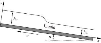
Consider a two-dimensional layer of liquid (see figure 1) of density
 ${\it\rho}$
and kinematic viscosity
 ${\it\nu}$
, on a substrate inclined at an angle
 ${\it\alpha}$
. Let the
 $x$
and
 $z$
axes be directed along, and perpendicular to, the substrate. The liquid’s free surface is described by the equation
 $z=h(x,t)$
, where
 $h$
is the layer’s depth and
 $t$
is the time. We also introduce the parallel-to-the-substrate and perpendicular-to-the-substrate components of the velocity,
 $u(x,z,t)$
and
 $w(x,z,t)$
, the pressure
 $p(x,z,t)$
, and the acceleration due to gravity
 $g$
.
The setting: a hydraulic jump (bore) on an inclined plate.

Let
 $H$
be the liquid’s characteristic depth, and
 $L$
and
 $U$
be the spatial scale and velocity (both in the
 $x$
direction). The following non-dimensional variables will be used:
 $$\begin{eqnarray}x_{\ast }=\frac{x}{L},\quad z_{\ast }=\frac{z}{H},\quad t_{\ast }=\frac{U}{L}t,\end{eqnarray}$$
 $$\begin{eqnarray}u_{\ast }=\frac{u}{U},\quad w_{\ast }=\frac{L}{UH}w,\quad p_{\ast }=\frac{p}{{\it\rho}Hg\cos {\it\alpha}},\quad h_{\ast }=\frac{h}{H}.\end{eqnarray}$$
We assume the stream-wise pressure gradient and viscosity to be of the same order, i.e.
 $$\begin{eqnarray}\frac{Hg\cos {\it\alpha}}{L}=\frac{{\it\nu}U}{H^{2}}.\end{eqnarray}$$
The problem is governed by three non-dimensional parameters: the characteristic ratio
 $Re$
of inertia and viscosity, the slope
 ${\it\varepsilon}$
of the free surface and the substrate’s non-dimensional slope
 $s$
,
 $$\begin{eqnarray}Re=\frac{UH^{2}}{L{\it\nu}},\quad {\it\varepsilon}=\frac{H}{L},\quad s=\frac{\tan {\it\alpha}}{{\it\varepsilon}}.\end{eqnarray}$$
Note that, in the context of shallow-water theories such as ours,
 $Re$
is often referred to as the ‘reduced Reynolds number’, emphasising the fact that it is equal to the ‘standard’ Reynolds number
 $UH/{\it\nu}$
multiplied by the small-slope parameter
 $H/L$
.
In terms of the non-dimensional variables (2.1)–(2.3), the Navier–Stokes equations for incompressible liquids are (asterisks omitted)
 $$\begin{eqnarray}\displaystyle & \displaystyle Re\left(\frac{\partial u}{\partial t}+u\frac{\partial u}{\partial x}+w\frac{\partial u}{\partial z}\right)+\frac{\partial p}{\partial x}=s+{\it\varepsilon}^{2}\frac{\partial ^{2}u}{\partial x^{2}}+\frac{\partial ^{2}u}{\partial z^{2}}, & \displaystyle\end{eqnarray}$$
 $$\begin{eqnarray}\displaystyle & \displaystyle {\it\varepsilon}^{2}Re\left(\frac{\partial w}{\partial t}+u\frac{\partial w}{\partial x}+w\frac{\partial w}{\partial z}\right)+\frac{\partial p}{\partial z}=-1+{\it\varepsilon}^{4}\frac{\partial ^{2}w}{\partial x^{2}}+{\it\varepsilon}^{2}\frac{\partial ^{2}w}{\partial z^{2}}, & \displaystyle\end{eqnarray}$$
 $$\begin{eqnarray}\displaystyle & \displaystyle \frac{\partial u}{\partial x}+\frac{\partial w}{\partial z}=0. & \displaystyle\end{eqnarray}$$
 $$\begin{eqnarray}u=0,\quad w=0\quad \text{at }z=0.\end{eqnarray}$$
At the free surface we impose the standard dynamic and kinematic conditions,
 $$\begin{eqnarray}\displaystyle & \displaystyle \frac{\partial u}{\partial z}+{\it\varepsilon}^{2}\frac{\partial w}{\partial x}-\left(2{\it\varepsilon}^{2}\frac{\partial u}{\partial x}-p\right)\frac{\partial h}{\partial x}=0\quad \text{at }z=h, & \displaystyle\end{eqnarray}$$
 $$\begin{eqnarray}\displaystyle & \displaystyle 2{\it\varepsilon}^{2}\frac{\partial w}{\partial z}-p-{\it\varepsilon}^{2}\left(\frac{\partial u}{\partial z}+{\it\varepsilon}^{2}\frac{\partial w}{\partial x}\right)\frac{\partial h}{\partial x}=0\quad \text{at }z=h, & \displaystyle\end{eqnarray}$$
 $$\begin{eqnarray}\displaystyle & \displaystyle \frac{\partial h}{\partial t}+u\frac{\partial h}{\partial x}=w\quad \text{at }z=h. & \displaystyle\end{eqnarray}$$
 $$\begin{eqnarray}{\it\varepsilon}^{2}\rightarrow 0.\end{eqnarray}$$
The inclination angle is assumed to be comparably small,
 ${\it\alpha}=O({\it\varepsilon})$
– in which case the definition of
 $s$
(see (2.4)) implies
 $$\begin{eqnarray}s=O(1).\end{eqnarray}$$
Physically, the smallness of
 ${\it\alpha}$
is required because an order-one slope of the substrate usually gives rise to an order-one slope of the free surface (the only exception is the limit where the elevation of the free surface is much smaller than the mean depth). Finally, we assume
 $$\begin{eqnarray}Re=O(1).\end{eqnarray}$$
As seen later, this assumption includes the limiting cases
 $Re\rightarrow 0$
and
 $Re\rightarrow \infty$
as well.
Now, letting
 ${\it\varepsilon}^{2}\rightarrow 0$
in (2.6) and (2.10), we obtain
 $$\begin{eqnarray}\displaystyle & \displaystyle \frac{\partial p}{\partial z}=-1, & \displaystyle\end{eqnarray}$$
 $$\begin{eqnarray}\displaystyle & \displaystyle p=0\quad \text{at }z=h, & \displaystyle\end{eqnarray}$$
 $$\begin{eqnarray}p=h-z.\end{eqnarray}$$
Using (2.17) to eliminate
 $p$
in the rest of the governing equations and taking the limit
 ${\it\varepsilon}^{2}\rightarrow 0$
, we obtain an asymptotic set of equations governing
 $u$
,
 $w$
and
 $h$
.
Before we present these equations, however, it is convenient to reduce the number of the parameters involved by setting
 $$\begin{eqnarray}Re=1.\end{eqnarray}$$
Note that this equality is applied after all small terms have been omitted from the governing equations – hence, it does not amount to an extra assumption or cause loss of generality. To see what it does do, substitute the definition of
 $Re$
(2.4) into (2.18) and take into account (2.3), which yields
 $$\begin{eqnarray}L^{2}=\frac{H^{5}g\cos {\it\alpha}}{{\it\nu}^{2}}.\end{eqnarray}$$
Thus, (2.18) relates the non-dimensionalisation scale
 $L$
to the other parameters.
Now, given (2.17)–(2.18), the limiting (
 ${\it\varepsilon}^{2}\rightarrow 0$
) form of (2.5), (2.7)–(2.9), (2.11) becomes
 $$\begin{eqnarray}\displaystyle & \displaystyle \frac{\partial u}{\partial t}+u\frac{\partial u}{\partial x}+w\frac{\partial u}{\partial z}+\frac{\partial h}{\partial x}=s+\frac{\partial ^{2}u}{\partial z^{2}}, & \displaystyle\end{eqnarray}$$
 $$\begin{eqnarray}\displaystyle & \displaystyle \frac{\partial u}{\partial x}+\frac{\partial w}{\partial z}=0, & \displaystyle\end{eqnarray}$$
 $$\begin{eqnarray}u=0,\quad w=0\quad \text{at }z=0,\end{eqnarray}$$
 $$\begin{eqnarray}\displaystyle & \displaystyle \frac{\partial u}{\partial z}=0\quad \text{at }z=h, & \displaystyle\end{eqnarray}$$
 $$\begin{eqnarray}\displaystyle & \displaystyle \frac{\partial h}{\partial t}+u\frac{\partial h}{\partial x}=w\quad \text{at }z=h. & \displaystyle\end{eqnarray}$$
To place (2.20)–(2.24) in the context of the existing models, we mention that:
-
(1) The Benney (Reference Benney1973) model for ideal fluids can be recovered from (2.20) to (2.24) by omitting the right-hand side of (2.20) (i.e. the viscous and inclination terms) and the first (no-slip) boundary condition in (2.22). Asymptotically, this corresponds to the limit
 $Re\rightarrow \infty$
.
Note also that, if
$u$
is independent of
$z$
and (2.25)the Benny model reduces to the standard shallow-water equations.
$$\begin{eqnarray}w=-z\frac{\partial u}{\partial x},\end{eqnarray}$$
-
(2) The lubrication approximation for flows on a slightly inclined plate can be recovered from (2.20) to (2.24) by omitting the first three (inertial) terms in (2.20). Asymptotically, this corresponds to the limit
$Re\rightarrow 0$
. -
(3) Equations similar to (2.20)–(2.24) have been used by Bohr, Putkaradze & Watanabe (Reference Bohr, Putkaradze and Watanabe1997) for stationary, radially symmetric jumps created by a vertical jet falling onto a horizontal substrate. Both models can be viewed as free-surface extensions of the classical boundary layer theory (see Schlichting Reference Schlichting1979).


3. Existence of steady bores
Hydraulic jumps (bores) are described by the following boundary conditions:
 $$\begin{eqnarray}h\rightarrow h_{\pm }\quad \text{as }x\rightarrow \pm \infty ,\end{eqnarray}$$
where
 $h_{-}$
(
 $h_{+}$
) is the liquid’s upstream (downstream) depth, such that
 $h_{-}>h_{+}$
.
Let
 $c$
be the bore’s non-dimensional speed relative to the substrate. To make the bore steady, assume that the substrate is moving in the opposite direction with the same speed, i.e. replace the boundary condition (2.22) with
 $$\begin{eqnarray}u=-c,\quad w=0\quad \text{at }z=0.\end{eqnarray}$$
Now the time derivatives in equations (2.20) and (2.24) can be omitted,
 $$\begin{eqnarray}\displaystyle & \displaystyle u\frac{\partial u}{\partial x}+w\frac{\partial u}{\partial z}+\frac{\partial h}{\partial x}=s+\frac{\partial ^{2}u}{\partial z^{2}}, & \displaystyle\end{eqnarray}$$
 $$\begin{eqnarray}\displaystyle & \displaystyle u\frac{\partial h}{\partial x}=w\quad \text{at }z=h. & \displaystyle\end{eqnarray}$$
 $x\rightarrow \pm \infty$
in (3.2)–(3.4), (2.21)–(2.23) and applying conditions (3.1), one obtains
 $$\begin{eqnarray}u\rightarrow -c+s(zh_{\pm }-{\textstyle \frac{1}{2}}z^{2}),\quad w\rightarrow 0\quad \text{as }x\rightarrow \pm \infty .\end{eqnarray}$$
It can be shown that the boundary-value problem (3.2)–(3.4), (2.21)–(2.23) complies with the mass conservation law, which implies
 $$\begin{eqnarray}\lim _{x\rightarrow -\infty }\int _{0}^{h}u\,\text{d}z=\lim _{x\rightarrow +\infty }\int _{0}^{h}u\,\text{d}z.\end{eqnarray}$$
Substituting into this equality the boundary conditions (3.1) and (3.5), one obtains
 $$\begin{eqnarray}c={\textstyle \frac{1}{3}}s(h_{-}^{2}+h_{-}h_{+}+h_{+}^{2}).\end{eqnarray}$$
Without loss of generality, one can set
 $h_{-}=1$
(which implies that the scale
 $H$
used in non-dimensionalisation (2.1)–(2.3) is the dimensional upstream depth). Thus, the problem at hand is fully determined by two parameters:
 $s$
and the downstream-to-upstream depth ratio
 ${\it\eta}$
(if
 $h_{-}=1$
, then
 ${\it\eta}=h_{+}$
).
3.1. The approach
A lot of information about steady bores can be extracted by examining the large-distance asymptotics of problem (3.2)–(3.4), (2.17)–(2.20). To do so, let
 $$\begin{eqnarray}u=-c+s(zh_{\pm }-{\textstyle \frac{1}{2}}z^{2})+\tilde{u} (x,z),\quad w=\tilde{w}(x,z),\quad h=h_{\pm }+\tilde{h}(x),\end{eqnarray}$$
where the tilded variables represent the deviations of the fields from their large-distance limits (3.1) and (3.5). Substituting (3.8) into (3.2)–(3.4) and (2.17)–(2.20), we linearise these with respect to
 $\tilde{u}$
,
 $\tilde{w}$
and
 $\tilde{h}$
. Then we let
 $$\begin{eqnarray}\tilde{u} =\hat{u} (z)\exp ({\it\lambda}x),\quad \tilde{w}={\hat{w}}(z)\exp ({\it\lambda}x),\quad \tilde{h}={\hat{h}}\exp ({\it\lambda}x)\end{eqnarray}$$
and, eliminating
 $\hat{u}$
and
 ${\hat{h}}$
, obtain
 $$\begin{eqnarray}\displaystyle & & \displaystyle \frac{1}{{\it\lambda}}\frac{\text{d}^{3}{\hat{w}}}{\text{d}z^{3}}+\left[c-s\left(h_{\pm }z-\frac{z^{2}}{2}\right)\right]\frac{\text{d}{\hat{w}}}{\text{d}z}+s(h_{\pm }-z){\hat{w}}=\frac{1}{s}\left(\frac{\text{d}^{2}{\hat{w}}}{\text{d}z^{2}}\right)_{z=h_{\pm }},\end{eqnarray}$$
 $$\begin{eqnarray}{\hat{w}}=0,\quad \frac{\text{d}{\hat{w}}}{\text{d}z}=0\quad \text{at }z=0,\end{eqnarray}$$
 $$\begin{eqnarray}\frac{1}{s}\left(c-\frac{sh_{\pm }^{2}}{2}\right)\frac{\text{d}^{2}{\hat{w}}}{\text{d}z^{2}}-{\hat{w}}=0\quad \text{at }z=h_{\pm }.\end{eqnarray}$$
Equations (3.10)–(3.12) form an eigenvalue problem – or, to be precise, two problems: one involving
 $h_{-}$
and the other involving
 $h_{+}$
. The two versions of (3.10)–(3.12) will be referred to as the upstream and downstream problems, with their eigenvalues denoted by
 ${\it\lambda}_{-}$
and
 ${\it\lambda}_{+}$
.
The large-distance expressions (3.8)–(3.9) comply with the boundary condition (3.1) only if
 $$\begin{eqnarray}Re{\it\lambda}_{-}>0,\quad Re{\it\lambda}_{+}<0,\end{eqnarray}$$
so such eigenvalues will be referred to as ‘good’.
It turns out that the existence criterion for steady bores can be derived by counting the ‘good’ and ‘bad’ eigenvalues of (3.10)–(3.12). In fact, it is sufficient to consider just two particular cases.
Case 1. If the downstream problem (i.e. (3.10)–(3.12) with
 $h_{+}$
) has no ‘good’ eigenvalues, no steady bores exist.
In this case, the governing equations simply do not have solutions such that
 $h\rightarrow h_{+}$
as
 $x\rightarrow +\infty$
.
Next, let the downstream problem have one good eigenvalue
 ${\it\lambda}_{+}$
, so that the downstream behaviour of, say,
 $h$
is
 $$\begin{eqnarray}h\sim h_{+}+{\hat{h}}\exp ({\it\lambda}_{+}x)\quad \text{as }x\rightarrow +\infty ,\end{eqnarray}$$
where
 ${\hat{h}}$
is a constant. Asymptotic (3.14) fixes a certain global solution, and we claim that it represents a steady bore (i.e. approaches
 $h_{-}$
as
 $x\rightarrow -\infty$
) only if all eigenvalues of the upstream problem are good. Indeed, even a single bad eigenvalue would drive the solution away from
 $h_{-}$
, and there are no ‘adjustment parameters’ to eliminate its contribution (changing
 ${\hat{h}}\rightarrow {\hat{h}}_{new}$
in (3.14) just shifts the solution along the
 $x$
axis as a whole by a distance of
 $\ln {\hat{h}}/{\hat{h}}_{new}$
).
The above argument amounts to the following claim:
Case 2. If the downstream problem has one ‘good’ eigenvalue, and its upstream counterpart has one or more ‘bad’ eigenvalues, no steady bores exist.
In general, if the downstream (upstream) problem has
 $n_{+}$
(
 $m_{-}$
) good (bad) eigenvalues, and
 $m_{-}\geqslant n_{+}$
, then no steady solutions exist.
We emphasise that Cases 1–2 should not be viewed as theorems, as they imply certain properties of the governing equations, which we have not proved. Asymptotic (3.8)–(3.9), for example, implies that the unknowns decay towards their limiting values exponentially, and no other decaying solutions exist – which is, strictly speaking, only an assumption.
Given that this work is mostly concerned with physical aspects of the bore dynamics, few rigorous proofs are presented. Our conclusions are supported by numerical and/or asymptotic solutions.
3.2. Properties of the eigenvalue problem (3.10)–(3.12)
In this subsection, seven propositions are formulated. The numbers of five of them are followed by the words ‘numerical’ or ‘asymptotic’, or both, implying that the corresponding proposition is supported by numerical and/or asymptotic evidence. The remaining two propositions are either proved rigorously or follow from the other propositions.
Proposition 1 (Numerical, asymptotic).
All eigenvalues of both up- and downstream problems are real.
This proposition has been verified numerically (using the shooting method) by a thorough parameter sweep of the
 $({\it\eta},s)$
plane. Only real eigenvalues have been found, and the Cauchy’s argument principle on the complex
 ${\it\lambda}$
plane was used to make sure that none of moderately large eigenvalues (
 $|{\it\lambda}|<500$
) was missed. Large eigenvalues, in turn, were found asymptotically using the WKB method (see appendix A), and they also turned out to be real.
Proposition 2. Both up- and downstream problems with
 ${\it\eta}<1$
never admit the zero eigenvalue.
This proposition can be proved by observing that, in the limit
 ${\it\lambda}\rightarrow 0$
, (3.10) can be easily solved. Its solution satisfies the boundary conditions (3.11)–(3.12) only for
 ${\it\eta}=1$
.
Propositions 1 and 2 imply that a finite change of
 ${\it\eta}$
or
 $s$
cannot ‘push’ a good eigenvalue through zero and thus make it bad, or vice versa. Good eigenvalues can only disappear (appear) by exiting through (coming from) infinity.
3.2.1. The downstream problem
Proposition 3 (Numerical, asymptotic).
The downflow problem has at most one ‘good’ eigenvalue.
This proposition has been verified numerically and by the WKB method. The latter yields (see appendix A)
 $$\begin{eqnarray}{\it\lambda}_{+}={\rm\pi}^{2}\left(n+\frac{1}{2}\right)^{2}\left[\int _{0}^{h_{+}}\sqrt{c-s\left(h_{+}z-\frac{1}{2}z^{2}\right)}\,\text{d}z\right]^{-2},\end{eqnarray}$$
where
 $n$
is an integer. Equation (3.15) is formally applicable for
 $n\gg 1$
, but in reality it agrees well with the numerical results for
 $n\geqslant 3$
.
Proposition 4 (Asymptotic).
If
 $$\begin{eqnarray}s^{2}>\frac{(2a_{+}-1)^{1/2}+2a_{+}\arctan [(2a_{+}-1)^{-1/2}]}{h_{+}^{3}(2a_{+}-1)^{3/2}a_{+}},\end{eqnarray}$$
where
 $a_{+}=c/sh_{+}^{2}$
all eigenvalues of the downflow problem are ‘bad’.
According to Propositions 1 and 2, good eigenvalues of the downflow problem can (dis)appear only by passing through the negative infinity. Thus, Proposition 4 can be proved by examining the limit
 ${\it\lambda}\rightarrow -\infty$
. It can be readily shown (see appendix B) that a large negative eigenvalue exists when
 $s^{2}$
is close to, but still smaller than, the threshold determined by the right-hand side of (3.16). When
 $s^{2}$
reaches the threshold, the eigenvalue goes to negative infinity and disappears. Finally, by virtue of Proposition 3, no more than one good eigenvalue can exist – so when it is gone, none is left.
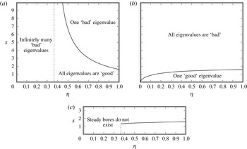
Proposition 4 is illustrated in figure 2(
 $b$
) (where the ‘
 $+$
’ indicates that this figure applies to the downstream problem, arising as
 $x\rightarrow +\infty$
).
The solutions of the upstream (a) and downstream (b) versions of the eigenvalue problem (3.10)–(3.12), on the
 $({\it\eta},s)$
plane.
 ${\it\eta}$
is the downstream-to-upstream depth ratio,
 $s$
is the substrate’s non-dimensional slope. The implications for the existence of bores are illustrated in panel (c). The solid curve in panels (
 $b$
) and (
 $c$
) correspond to criterion (3.16), the dotted straight lines in panels (
 $a$
) and (
 $c$
) correspond to the condition
 ${\it\eta}=(\sqrt{3}-1)/2$
. The solid curve in panel (
 $a$
) corresponds to criterion (3.19), but since this curve lies above the solid curve in panel (
 $b$
), it does not affect the existence of bores.

3.2.2. The upstream problem
It turns out that the properties of the upstream problem depend on whether or not
 ${\it\eta}$
is smaller than a certain critical value,
 $$\begin{eqnarray}{\it\eta}_{cr}={\textstyle \frac{1}{2}}(\sqrt{3}-1).\end{eqnarray}$$
To understand the significance of
 ${\it\eta}_{cr}$
, observe that, if
 ${\it\eta}>{\it\eta}_{cr}$
, the upstream velocity profile (3.5) is sign-definite. If, on the other hand,
 ${\it\eta}<{\it\eta}_{cr}$
, a level of zero velocity
 $z_{0}$
exists in the upstream region, i.e.
 $$\begin{eqnarray}c-s(h_{-}z_{0}-{\textstyle \frac{1}{2}}z_{0}^{2})=0,\quad z_{0}\in (0,h_{-}).\end{eqnarray}$$
Proposition 5 (Numerical, asymptotic).
If
 ${\it\eta}>{\it\eta}_{cr}$
, all eigenvalues of the upstream problem are.‘good’ except, maybe, one. The only bad eigenvalue exists if and only if
 $$\begin{eqnarray}s^{2}>\frac{(2a_{-}-1)^{1/2}+2a_{-}\arctan [(2a_{-}-1)^{-1/2}]}{h_{-}^{3}(2a_{-}-1)^{3/2}a_{-}},\end{eqnarray}$$
where
 $a_{-}=c/sh_{-}^{2}$
.
This proposition has been verified by solving (3.10)–(3.12) numerically and asymptotically via the WKB method (see appendix A.2). Condition (3.19) can be verified in a similar way to its downflow counterpart (3.16) (the latter is examined in appendix B). It turns out, however, that condition (3.19) is unimportant, as it is less strict than (3.16). As a result, when a bad
 ${\it\lambda}_{-}$
emerges, all of
 ${\it\lambda}_{+}$
are already bad – so no bores exists anyway according to Case 1.
Proposition 6 (Asymptotic).
If
 $$\begin{eqnarray}{\it\eta}<{\it\eta}_{cr},\end{eqnarray}$$
the upflow problem has infinitely many ‘bad’ eigenvalues.
This proposition has been verified through the WKB method, which yields two infinite sequences of eigenvalues – one going to positive infinity and the other to negative infinity. As shown in appendix A.2, the latter (bad) eigenvalues are
 $$\begin{eqnarray}{\it\lambda}_{+}=-{\rm\pi}^{2}\left(n+\frac{1}{4}\right)^{2}\left[\int _{z_{0}}^{h_{-}}\sqrt{c-s\left(h_{-}z-\frac{1}{2}z^{2}\right)}\,\text{d}z\right]^{-2}.\end{eqnarray}$$

3.3. The non-existence conditions for bores
The implications of the properties of the up- and downflow problems (3.10)–(3.12) for existence of steady bores can be summarised as follows:
Proposition 7. If either of conditions (3.16) or (3.20) holds, the governing equations (2.20)–(2.24) do not have solutions for steady bores.
This proposition is illustrated in figure 2(
 $c$
), where the results presented in figures 2(
 $a$
) and 2(
 $b$
) are merged.
4. Examples and discussion
Recall that all results obtained so far apply to the non-existence of steady bores in various regions of the
 $({\it\eta},s)$
plane, and it remains unclear whether they exist in the rest of the plane. This question has been clarified numerically, with the results suggesting that bores do exist unless there is a ‘reason’ for them not to. Numerical results will also help us to determine the physical mechanisms eliminating bores as steady solutions.
In what follows, we shall first rewrite the asymptotic equations (2.20)–(2.24) in terms of the (more convenient) semi-Lagrangian variables. Then we shall present and discuss the numerical results obtained.
4.1. Semi-Lagrangian variables
The main difficulty when simulating free-surface flows stems from the fact that the computational domain has an a priori unknown, moving boundary. This difficulty can be bypassed by using semi-Lagrangian variables, such that the perpendicular-to-the-substrate coordinate is replaced by a Lagrangian marker, whereas the parallel-to-the-substrate coordinate remains Eulerian. These variables have been previously used by Odulo (Reference Odulo1979) and Zakharov (Reference Zakharov1981) for analyses of shallow-water models similar to ours.
Let
 $(t_{new},x_{new},{\it\xi})$
be new variables related to the Eulerian coordinates
 $(t,x,z)$
by
 $$\begin{eqnarray}t=t_{new},\quad x=x_{new},\quad z=z(t_{new},x_{new},{\it\xi}),\end{eqnarray}$$
with
 $z$
satisfying (the subscript
 $_{new}$
omitted)
 $$\begin{eqnarray}\displaystyle & \displaystyle \frac{\partial z}{\partial t}+u\frac{\partial z}{\partial x}-w=0, & \displaystyle\end{eqnarray}$$
 $$\begin{eqnarray}\displaystyle & \displaystyle z=0\quad \text{at }{\it\xi}=0, & \displaystyle\end{eqnarray}$$
 $$\begin{eqnarray}\displaystyle & \displaystyle z=h\quad \text{at }{\it\xi}=1. & \displaystyle\end{eqnarray}$$
 ${\it\xi}$
is the Lagrangian marker corresponding to the Eulerian coordinate
 $z$
. Conditions (4.3)–(4.4) make the substrate and free surface correspond to
 ${\it\xi}=0$
and
 ${\it\xi}=1$
. Observe that (4.2)
 $_{{\it\xi}=1}$
coincides with (2.24) – hence, the latter can be omitted.
Rewriting (2.20)–(2.23) in terms of
 $(t_{new},x_{new},{\it\xi})$
and taking into account (4.2), we obtain (the subscript
 $_{new}$
omitted)
 $$\begin{eqnarray}\displaystyle & \displaystyle \frac{\partial u}{\partial t}+u\frac{\partial u}{\partial x}+\frac{\partial }{\partial x}\int _{0}^{1}z^{\prime }\,\text{d}{\it\xi}=s+\frac{1}{z^{\prime }}\frac{\partial }{\partial {\it\xi}}\left(\frac{1}{z^{\prime }}\frac{\partial u}{\partial {\it\xi}}\right), & \displaystyle\end{eqnarray}$$
 $$\begin{eqnarray}\displaystyle & \displaystyle \frac{\partial u}{\partial x}z^{\prime }+\frac{\partial w}{\partial y}z^{\prime }-\frac{\partial z}{\partial x}\frac{\partial u}{\partial {\it\xi}}-\frac{\partial z}{\partial y}\frac{\partial w}{\partial {\it\xi}}+\frac{\partial w}{\partial {\it\xi}}=0, & \displaystyle\end{eqnarray}$$
 $$\begin{eqnarray}\displaystyle & \displaystyle u=0\quad \text{at }{\it\xi}=0, & \displaystyle\end{eqnarray}$$
 $$\begin{eqnarray}\displaystyle & \displaystyle \frac{\partial u}{\partial {\it\xi}}=0\quad \text{at }{\it\xi}=1, & \displaystyle\end{eqnarray}$$
 $$\begin{eqnarray}z^{\prime }=\frac{\partial z}{\partial {\it\xi}}.\end{eqnarray}$$
Now, differentiate (4.2) with respect to
 ${\it\xi}$
and add the result to (4.6), which yields
 $$\begin{eqnarray}\frac{\partial z^{\prime }}{\partial t}+\frac{\partial (uz^{\prime })}{\partial x}=0.\end{eqnarray}$$
Equations (4.5) and (4.10) and the boundary conditions (4.7)–(4.8) govern
 $u$
and
 $z^{\prime }$
(
 $w$
and
 $z$
have been eliminated). As expected, the unknowns are to be determined in a fixed domain,
 $(x,{\it\xi})\in (-\infty ,+\infty )\times (0,1)$
.
For steady solutions, (4.5) and (4.10) yield
 $$\begin{eqnarray}\displaystyle & \displaystyle \frac{\partial }{\partial x}\left(\frac{u^{2}}{2}+\int _{0}^{1}z^{\prime }\,\text{d}{\it\xi}\right)=s+\frac{1}{z^{\prime }}\frac{\partial }{\partial {\it\xi}}\left(\frac{1}{z^{\prime }}\frac{\partial u}{\partial {\it\xi}}\right), & \displaystyle\end{eqnarray}$$
 $$\begin{eqnarray}\displaystyle & \displaystyle u\,z^{\prime }=F, & \displaystyle\end{eqnarray}$$
 $F({\it\xi})$
is, physically, the flux along the streamlines. It can be fixed by taking the limit
 $x\rightarrow +\infty$
. Exploiting the fact that Lagrangian markers can be assigned arbitrarily at the ‘entrance’ of the flow, let
 $$\begin{eqnarray}z=h_{+}{\it\xi}\quad \text{as }x\rightarrow +\infty\end{eqnarray}$$
and thus rewrite the downstream version of (3.5) in the form
 $$\begin{eqnarray}u\rightarrow -c+sh_{+}^{2}({\it\xi}-{\textstyle \frac{1}{2}}{\it\xi}^{2})\quad \text{as }x\rightarrow +\infty .\end{eqnarray}$$
Equations (4.9) and (4.12)–(4.14) yield
 $$\begin{eqnarray}F=h_{+}[-c+sh_{+}^{2}({\it\xi}-{\textstyle \frac{1}{2}}{\it\xi}^{2})].\end{eqnarray}$$
Equations (4.11)–(4.12), (4.15) and conditions (4.7)–(4.8), (4.14) fully determine
 $u$
and
 $z^{\prime }$
.
Observe that the set of equations to be solved is of the first order in
 $x$
. Hence, it can be integrated with respect to
 $x$
‘in a single sweep’ from
 $+\infty$
to
 $-\infty$
, with (4.14) playing the role of the initial condition.
4.2. The numerical method
Solutions of the steady problem (4.11)–(4.12), (4.14)–(4.15) and (4.7)–(4.8) were computed using a simple finite-difference scheme, based on a two-point implicit approximation of the
 $x$
derivative in (4.11), three-point central approximation of the
 ${\it\xi}$
derivative and the trapezoid rule for the integral. For
 ${\it\eta}$
close to
 ${\it\eta}_{cr}$
, an extra fine mesh was used near
 ${\it\xi}=1$
. This was necessary because the solution is expected to have the following property:
 $$\begin{eqnarray}(z^{\prime })_{{\it\xi}=1,x=-\infty }\rightarrow \infty \quad \text{as }{\it\eta}\rightarrow {\it\eta}_{cr}.\end{eqnarray}$$
Equation (4.16) follows from (4.12), (4.15) and the fact that
 $(u)_{{\it\xi}=1,x=-\infty }\rightarrow 0$
as
 ${\it\eta}\rightarrow {\it\eta}_{cr}$
.
4.3. The results
A thorough sweep of the
 $({\it\eta},s)$
plane was carried out, and solutions were found in the whole of the region where their existence was not ruled out (see figure 2(
 $c$
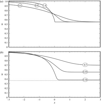
)). Some typical examples of bores are shown in figure 3.
Examples of steady bores: (a) a sequence of bores approaching the upper boundary of the existence region (shown in figure 2(
 $c$
)) (
 $s=0.4$
, 0.8, 1.4;
 ${\it\eta}=0.55$
); (b) a sequence of bores approaching the left boundary of the existence region. The dotted line in panel (b) corresponds to the limiting value of
 $h_{+}$
below which no solutions exist for the given
 $h_{-}$
(
 $s=0.8$
,
 ${\it\eta}=0.7$
, 0.55, 0.38).

Figure 3(a) shows three bores with increasing values of the substrate’s non-dimensional slope
 $s$
, but the same upflow-to-downflow depth ratio
 ${\it\eta}$
. One can see that a ‘corner’ develops at the foot of the bore’s front, and the tangent there becomes vertical. It can be assumed that, for steeper slopes, all bores overturn.
Figure 3(b), in turn, shows three bores with the same
 $s$
, but decreasing values of
 ${\it\eta}$
(i.e. with increasing relative amplitudes). Interestingly, the free surface in this case remains smooth no matter how close
 ${\it\eta}$
is to
 ${\it\eta}_{cr}$
. Note also that singularity (4.16) is an artefact of the semi-Lagrangian variables, and in terms of the original Eulerian coordinates all fields are smooth. Thus, the bores do not disappear due to a singularity of the solution.
We shall not discuss this issue in further detail, but refer the reader to Benilov & Lapin (Reference Benilov and Lapin2015), who examined steady bores in the limit
 $Re\ll 1$
,
 ${\it\varepsilon}\sim 1$
. It was shown that, in this case, bores disappear at exactly the same critical value
 ${\it\eta}_{cr}$
(given by (3.17)), due to a stagnation point emerging at
 $x=-\infty$
. Exactly the same effect occurs in the present setting as well.
Several other features of bores are worth observing:
-
(i) In the framework of the lubrication approximation (LA), steady bores exist for all values of
$s$
and
$h_{\pm }$
– which clearly contradicts our results. To explain the contradiction, observe that the non-existence region described by condition (3.16) corresponds to order-one Reynolds number and, thus, the LA is not applicable there. As for the non-existence region described by condition (3.17), the LA is applicable to its small-
$s$
part and, thus, predicts ‘ghost’ (non-existing) solutions there. This occurs because it does not capture the essential dynamics near stagnation points (for more details, see Benilov & Lapin Reference Benilov and Lapin2015).One has probably a better chance of capturing this dynamics using a model with a more refined approximation than the LA approximation of the flow’s vertical structure (Bohr et al. Reference Bohr, Putkaradze and Watanabe1997; Ruyer-Quil & Manneville Reference Ruyer-Quil and Manneville2000, Reference Ruyer-Quil and Manneville2002; Weinstein & Ruschak Reference Weinstein and Ruschak2004; Luchini & Charru Reference Luchini and Charru2010; Rojas et al. Reference Rojas, Argentina, Cerda and Tirapegui2010). It would be interesting to explore the existence of steady bores governed by these models.
-
(ii) Recall that our asymptotic model requires that the slope of the free surface be small – which, clearly, does not hold near the ‘corner’ emerging when
$s$
approaches its limiting value. Note, however, even though the computed shapes of near-limiting solutions cannot be trusted, the (intuitively correct) tendency of bore steepening for steeper inclines should still be. -
(iii) Evidently, the solutions presented in figure 3 are monotonic (as well as all examples computed for, but not included in, the paper) – whereas bores computed by Bertozzi et al. (Reference Bertozzi, Münch, Shearer and Zumbrun2001) and Benilov & Lapin (Reference Benilov and Lapin2011) have oscillatory structure. To resolve the discrepancy, recall that the latter authors observed oscillatory bores only for order-one inclination angles, whereas for slight angles the solution was monotonic. The ripples in the solution of Bertozzi et al. (Reference Bertozzi, Münch, Shearer and Zumbrun2001), in turn, were due to capillary effects (which we neglect).
-
(iv) Given the above, we shall quantify the negligibility of capillary effects. Rederiving (2.20)–(2.24) with surface tension included, one obtains (details omitted) the following generalisation of (2.20):
(4.17)with
$$\begin{eqnarray}\frac{\partial u}{\partial t}+u\frac{\partial u}{\partial x}+w\frac{\partial u}{\partial z}+\frac{\partial }{\partial x}\left(h-{\it\gamma}\frac{\partial ^{2}h}{\partial x^{2}}\right)=s+\frac{\partial ^{2}u}{\partial z^{2}},\end{eqnarray}$$
(4.18)where
$$\begin{eqnarray}{\it\gamma}=\frac{{\it\sigma}}{{\it\rho}L^{2}g\cos {\it\alpha}},\end{eqnarray}$$
${\it\sigma}$
is the surface tension and
$L$
is the stream-wise spatial scale. The inequality
${\it\gamma}\ll 1$
can be viewed as the condition that capillary effects are negligible, and it holds for most liquids if
$L$
exceeds 4–6 mm.
Note, however, that, even if the bore’s global horizontal scale is large, the local scale near a ‘corner’ is infinitely small. Hence, surface tension is always important for near-limiting solutions.
In principle, capillary effects can prevent the bore from overturning, but the results of Benilov & Lapin (Reference Benilov and Lapin2011) (obtained for the small-
$Re$
limit) suggest that, no matter how large
${\it\gamma}$
is, bores still overturn for a sufficiently steep incline. Thus, surface tension can ‘delay’ overturning, but cannot stop it altogether. Either way, the effect of surface tension on overturning bores is worth further investigation.


5. Summary and concluding remarks
Thus, we have examined the existence of hydraulic jumps (bores) with a small slope of the free surface and unrestricted Reynolds number, in a flow down an slightly inclined substrate. Our main result is Proposition 7 in § 3.3, illustrated in figure 2(
 $c$
). We have also clarified the physical mechanisms eliminating bores (§ 4.3 and figure 3).
It is worth rewriting our main result in terms of measurable (dimensional) parameters.
To do so, let the depth scale
 $H$
be the dimensional upstream depth
 $H_{-}$
. Then use (2.3) to express
 $U$
in terms of the other parameters and substitute it and (2.19) into the definitions of
 $s$
(2.4), which yields
 $$\begin{eqnarray}s^{2}=\frac{(H_{-})^{3}g\sin ^{2}{\it\alpha}}{{\it\nu}^{2}\cos {\it\alpha}}.\end{eqnarray}$$
The downflow-to-upflow depth ratio should also be expressed in terms of the dimensional parameters,
 $$\begin{eqnarray}{\it\eta}=\frac{H_{+}}{H_{-}},\end{eqnarray}$$
where
 $H_{+}$
is the flow’s downstream depth.
Note that our results have been so far formulated as conditions of non-existence of steady bores. Since it is more convenient to work with existence conditions, we shall replace inequalities (3.16) and (3.20) with their opposites.
Rewriting the opposite of condition (3.16) using (5.1)–(5.2), we obtain
 $$\begin{eqnarray}\frac{(H_{+})^{3}g\sin ^{2}{\it\alpha}}{{\it\nu}^{2}\cos {\it\alpha}}<\frac{(2a_{+}-1)^{1/2}+2a_{+}\arctan [(2a_{+}-1)^{-1/2}]}{(2a_{+}-1)^{3/2}a_{+}},\end{eqnarray}$$
where
 $$\begin{eqnarray}a_{+}=\frac{1}{3}\left[\left(\frac{H_{-}}{H_{+}}\right)^{2}+\frac{H_{-}}{H_{+}}+1\right].\end{eqnarray}$$
The opposite of condition (3.20), (3.17), in turn, can be rewritten in the form
 $$\begin{eqnarray}\frac{H_{+}}{H_{-}}>\frac{1}{2}(\sqrt{3}-1).\end{eqnarray}$$
Conditions (5.3)–(5.5) form the desired necessary and sufficient criterion of existence of steady bores.
Note that our asymptotic equations (2.20)–(2.24), as well as their semi-Lagrangian counterparts, can be readily extended to three-dimensional flows with surface tension and bottom topography.
Acknowledgements
The author acknowledges the support of the Science Foundation Ireland under grants 11/RFP.1/MTH3281 and 12/IA/1683.
Appendix A. The WKB analysis of (3.10)–(3.12)
In what follows, we assume that the solutions of the eigenvalue problem (3.10)–(3.12) are such that
 $(\text{d}^{2}{\hat{w}}/\text{d}z^{2})_{z=h_{\pm }}\neq 0$
(which has been verified numerically, through a thorough parameter sweep of the
 $({\it\eta},s)$
plane). Then, in view of the homogeneity of the problem, we can set
 $(\text{d}^{2}{\hat{w}}/\text{d}z^{2})_{z=h_{\pm }}=1$
and, thus, rewrite (3.10)–(3.12) as (the subscripts and hats omitted)
 $$\begin{eqnarray}\frac{1}{{\it\lambda}}\frac{\text{d}^{3}w}{\text{d}z^{3}}+\left[c-s\left(hz-\frac{z^{2}}{2}\right)\right]\frac{\text{d}w}{\text{d}z}+s(h-z)w=\frac{1}{s},\end{eqnarray}$$
 $$\begin{eqnarray}w=0,\quad \frac{\text{d}w}{\text{d}z}=0\quad \text{at }z=0,\end{eqnarray}$$
 $$\begin{eqnarray}\frac{1}{s}\left(c-\frac{sh^{2}}{2}\right)-w=0,\quad \frac{\text{d}^{2}w}{\text{d}z^{2}}=1\quad \text{at }z=h.\end{eqnarray}$$
It turns out that the solution depends on whether or not there exists a level of zero velocity
 $z_{0}$
, such that
 $$\begin{eqnarray}c-s(hz_{0}-{\textstyle \frac{1}{2}}z_{0}^{2})=0.\end{eqnarray}$$
 $z_{0}$
is, essentially, a turning point, and it gives rise to two families of solutions. One consists of eigenfunctions that oscillate in the interval
 $(0,z_{0})$
and are smooth in
 $(z_{0},h)$
, with the corresponding eigenvalues being positive. The eigenfunctions from the other family, in turn, oscillate only in
 $(z_{0},h)$
and have
 ${\it\lambda}<0$
. Finally, in the absence of the turning point, the eigenfunctions oscillate in the whole interval
 $(0,h)$
and all eigenvalues are positive.
We shall first examine flows without a level of zero velocity – i.e. upstream flows with
 ${\it\eta}>{\it\eta}_{cr}=(\sqrt{3}-1)/2$
and all of the downstream flows. Then we examine upstream flows with
 ${\it\eta}<{\it\eta}_{cr}$
for which
 $z_{0}$
does exist.
A.1. Flows without a level of zero velocity
Unlike the WKB solutions of second-order equations, those of the (third-order) problem (A 1)–(A 3) include both ‘fast’ and ‘slow’ components,
 $$\begin{eqnarray}w=W+w_{1}.\end{eqnarray}$$
In the limit
 $|{\it\lambda}|\gg 1$
, the slow component
 $w_{1}$
satisfies the following approximation of (A 1):
 $$\begin{eqnarray}O({\it\lambda}^{-1})+\left[c-s\left(hz-\frac{1}{2}{\it\xi}^{2}\right)\right]\frac{\text{d}w}{\text{d}z}+s(h-z)w=\frac{1}{s},\end{eqnarray}$$
which yields
 $$\begin{eqnarray}w_{1}=\left[c-s\left(hz-\frac{1}{2}z^{2}\right)\right]\left\{D+\int _{0}^{z}\frac{\text{d}{\it\xi}}{s[c-s(h{\it\xi}-{\textstyle \frac{1}{2}}{\it\xi}^{2})]^{2}}\right\}+O({\it\lambda}^{-1}),\end{eqnarray}$$
where
 $D$
is a constant of integration.
The fast component will be sought in the form
 $$\begin{eqnarray}W=Q(z)\cos \left[{\it\lambda}^{1/2}\int _{0}^{z}P({\it\xi})\,\text{d}{\it\xi}+B\right]+O({\it\lambda}^{-1}),\end{eqnarray}$$
where
 $B$
is an undetermined constant and
 ${\it\lambda}$
is implied to be real and positive (as we assumed for flows without a level of zero velocity). Substituting (A 5) into the homogeneous version of (A 1) and taking into account the zeroth and first orders of the expansion in
 ${\it\lambda}^{-1/2}$
, we obtain
 $$\begin{eqnarray}P=[c-s(hz-{\textstyle \frac{1}{2}}z^{2})]^{1/2},\quad Q=A[c-s(hz-{\textstyle \frac{1}{2}}z^{2})]^{-5/2},\end{eqnarray}$$
where
 $A$
is an arbitrary constant.
Substitution of solution (A 5)–(A 9) into the boundary conditions (A 2)–(A 3) yields four equations for
 $D$
,
 $B$
,
 $A$
and
 ${\it\lambda}$
, and it can be readily shown that, to leading order,
 ${\it\lambda}$
is given by (3.15).
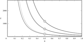
The asymptotic solution (3.15) is compared to the numerical solution of the exact eigenvalue problem in figure 4. One can see that (3.15) is fairly accurate even for the third eigenvalue (for higher eigenvalues, its accuracy can only improve).


A.2. Flows with a level of zero velocity
As mentioned above, there are two families of eigenfunctions in this case: those with
 ${\it\lambda}>0$
and those with
 ${\it\lambda}<0$
. The former will be examined first.
For the case
 ${\it\lambda}>0$
, seek a solution in the form
 $$\begin{eqnarray}\displaystyle w=\left[c-s\left(hz-\frac{1}{2}{\it\xi}^{2}\right)\right]\left\{D_{1}+\int _{0}^{z}\!\frac{\text{d}{\it\xi}}{s[c-s(h{\it\xi}-{\textstyle \frac{1}{2}}{\it\xi}^{2})]^{2}}\!\right\}+\,W+O({\it\lambda}^{-1})\quad \text{if }z<z_{0}, & & \displaystyle \nonumber\\ \displaystyle & & \displaystyle\end{eqnarray}$$
 $$\begin{eqnarray}\displaystyle w=\left[c-s\left(hz-\frac{1}{2}{\it\xi}^{2}\right)\right]\left\{D_{2}-\int _{z}^{h}\frac{\text{d}{\it\xi}}{s[c-s(h{\it\xi}-{\textstyle \frac{1}{2}}{\it\xi}^{2})]^{2}}\right\}+O({\it\lambda}^{-1})\quad \text{if }z>z_{0}, & & \displaystyle \nonumber\\ \displaystyle & & \displaystyle\end{eqnarray}$$
where the fast component
 $W$
is given by formulae (A 8)–(A 9). Substitution of (A 10) into the boundary conditions (A 1) yields
 $$\begin{eqnarray}B=0,\quad D_{1}=-Ac^{-9/4}.\end{eqnarray}$$
Solution (A 11), in turn, cannot satisfy both boundary conditions (A 3), which indicates that there is a boundary layer at
 $z=h$
. We shall not discuss it, however, as it does not affect the leading-order eigenvalue (and is similar to the boundary layer at
 $z=h$
of the solution examined in appendix B).
Observe that solutions (A 10) and (A 11) do not match at
 $z_{0}$
, as it can be shown that
 $$\begin{eqnarray}\displaystyle w & {\sim} & \displaystyle \frac{A{\it\lambda}^{5/12}}{[s(h-z_{0})]^{5/6}(-y)^{5/4}}\cos \left\{{\it\lambda}^{1/2}\int _{0}^{z_{0}}\left[c-s\left(hz-\frac{1}{2}z^{2}\right)\right]^{1/2}\,\text{d}z-\frac{2}{3}(-y)^{3/2}\right\}\nonumber\\ \displaystyle & & \displaystyle +\,\frac{1}{s^{2}(h-z_{0})}\quad \text{as }z\rightarrow z_{0}-0,\end{eqnarray}$$
 $$\begin{eqnarray}w\sim \frac{1}{s^{2}(h-z_{0})}\quad \text{as }z\rightarrow z_{0}+0,\end{eqnarray}$$
where
 $$\begin{eqnarray}y=[{\it\lambda}s(h-z_{0})]^{1/3}(z_{0}-z).\end{eqnarray}$$
The mismatch between (A 13) and (A 14) indicates that a boundary layer exists at
 $z_{0}$
.
To examine it, rewrite (A 1) in terms of
 $y$
(which is actually the inner variable) and keep the leading-order terms only, which yields
 $$\begin{eqnarray}\frac{\text{d}^{3}w_{i}}{\text{d}y^{3}}-y\frac{\text{d}w_{i}}{\text{d}y}+w_{i}=\frac{1}{s^{2}(h-z_{0})},\end{eqnarray}$$
where the subscript
 $_{i}$
stands for ‘inner’. Making two successive changes of variables,
 $w\rightarrow f_{1}\rightarrow f_{2}$
, such that
 $$\begin{eqnarray}w=yf_{1}+\frac{1}{s^{2}(h-z_{0})},\quad \frac{\text{d}f_{1}}{\text{d}y}=\frac{1}{y^{2}}\frac{\text{d}f_{2}}{\text{d}y},\end{eqnarray}$$
one can reduce (A 16) to the Airy equation for
 $f_{2}$
. Using then the properties of the Airy functions, one can show that all bounded solutions of the original equation (A 16) have the following large-distance asymptotics:
 $$\begin{eqnarray}w_{i}\sim \frac{1}{s^{2}(h-z_{0})}+c_{1}\frac{\sin [{\textstyle \frac{1}{4}}{\rm\pi}+{\textstyle \frac{2}{3}}(-y)^{2/3}]}{(-y)^{5/4}}\quad \text{as }{\it\xi}\rightarrow -\infty ,\end{eqnarray}$$
where
 $c_{1}$
is an undetermined constant. Finally, comparison of (A 18) to (A 13) yields
 $$\begin{eqnarray}{\it\lambda}^{1/2}\int _{0}^{z_{0}}\left[c-s\left(hz-\frac{1}{2}z^{2}\right)\right]^{1/2}\text{d}z=\left(\frac{1}{4}+n\right){\rm\pi},\end{eqnarray}$$
where
 $n>0$
is an integer. Equation (A 19) is, essentially, an expression for
 ${\it\lambda}$
.
To find negative eigenvalues, one should ‘interchange’ expressions (A 10) and (A 11), i.e. the fast component should be present in the region
 $z>z_{0}$
. The rest of the calculation remains virtually the same and, instead of (A 19), it yields (3.20).
Appendix B. The derivation of condition (3.16)
As described in the main body of the paper, condition (3.16) can be obtained by examining the values of
 $s$
for which
 ${\it\lambda}$
tends to negative infinity.
It should be emphasised that large eigenvalues do not necessarily correspond to fast-oscillating eigenfunctions as the WKB eigenvalues do (see appendix A). Note also that, even though the WKB eigenvalues are large, they cannot become infinitely large in response to a finite change of
 $s$
(as can be readily verified using expressions (3.15), (A 19) and (3.20)).
Thus, we assume that
 ${\it\lambda}$
is large, but
 $w(z)$
has non-oscillatory structure. Fast changes in
 $w(z)$
occur only near
 $z=0$
and
 $z=h$
, due to boundary layers located there (as before,
 $h$
and
 $w$
are stripped of subscripts and hats).
Outside the boundary layers, the solution can be obtained by omitting the first term in (A 1), which yields
 $$\begin{eqnarray}w=\left[c-s\left(hz-\frac{1}{2}z^{2}\right)\right]\left\{D+\int _{0}^{z}\frac{\text{d}{\it\xi}}{s[c-s(h{\it\xi}-{\textstyle \frac{1}{2}}{\it\xi}^{2})]^{2}}\right\}+O({\it\lambda}^{-1}).\end{eqnarray}$$
This expression coincides with the slow component (A 7) of the WKB solution, but the two solutions involve different values of the constant of integration.
The left-hand boundary layer (near
 $z=0$
) is described by the following inner variables:
 $$\begin{eqnarray}z_{l}=(-{\it\lambda})^{1/2}z,\quad w_{l}=(-{\it\lambda})^{1/2}w,\end{eqnarray}$$
where it is implied that
 ${\it\lambda}$
is real and negative (as any ‘good’ eigenvalue of the downflow problem should be). In terms of variables (B 2), (A 1) and boundary conditions (A 2) become
 $$\begin{eqnarray}-\frac{\text{d}^{3}w_{l}}{\text{d}z_{l}^{3}}+[c-(-{\it\lambda})^{-1/2}shz_{l}+O({\it\lambda}^{-1})]\frac{\text{d}w_{l}}{\text{d}z_{l}}+(-{\it\lambda})^{-1/2}shw_{l}=\frac{1}{s},\end{eqnarray}$$
 $$\begin{eqnarray}w_{l}=0,\quad \frac{\text{d}w_{l}}{\text{d}z_{l}}=0\quad \text{at }z_{l}=0.\end{eqnarray}$$
Seeking a solution in the form
 $w_{l}=w_{l}^{(0)}+(-{\it\lambda})^{-1/2}w_{l}^{(1)}+O({\it\lambda}^{-1})$
, one can readily obtain
 $$\begin{eqnarray}\displaystyle w_{l} & = & \displaystyle \frac{z_{l}}{sc}+\frac{\exp (-c^{1/2}z_{l})-1}{sc^{3/2}}+\frac{(-{\it\lambda})^{-1/2}h}{c}\nonumber\\ \displaystyle & & \displaystyle \times \,\left[\frac{\exp (-c^{1/2}z_{l})-1}{c}+\frac{z_{l}}{c^{1/2}}+\frac{z_{l}^{2}\exp (-c^{1/2}z_{l})}{3c}\right]+O({\it\lambda}^{-1}).\qquad\end{eqnarray}$$
Matching (B 5), (B 2) to the outer solution (B 1), we obtain
 $$\begin{eqnarray}D=-(-{\it\lambda})^{-1/2}\frac{1}{sc^{5/2}}.\end{eqnarray}$$
The right-hand boundary layer (the one near
 $z=h$
) is described by
 $$\begin{eqnarray}z_{r}=(-{\it\lambda})^{1/2}(z-h),\quad w_{r}=(-{\it\lambda})^{1/2}w,\end{eqnarray}$$
 $$\begin{eqnarray}-\frac{\text{d}^{3}w_{r}}{\text{d}z_{r}^{3}}+\left(c-\frac{sh^{2}}{2}\right)\frac{\text{d}w_{r}}{\text{d}z_{r}}=\frac{(-{\it\lambda})^{-1/2}}{s}+O({\it\lambda}^{-1}),\end{eqnarray}$$
 $$\begin{eqnarray}w_{r}=\frac{1}{s}\left(c-\frac{sh^{2}}{2}\right),\quad \frac{\text{d}^{2}w_{r}}{\text{d}z_{r}^{2}}=O({\it\lambda}^{-1})\quad \text{at }z_{r}=0,\end{eqnarray}$$
which yields
 $$\begin{eqnarray}w_{r}=\frac{1}{s}\left(c-\frac{sh^{2}}{2}\right)+\frac{(-{\it\lambda})^{-1/2}z_{r}}{s\left(c-\displaystyle \frac{sh^{2}}{2}\right)}+O({\it\lambda}^{-1}).\end{eqnarray}$$
Matching (B 10), (B 7) to the outer solution (B 1), we obtain
 $$\begin{eqnarray}\sqrt{-{\it\lambda}}=c^{5/2}\left\{\int _{0}^{h}\frac{\text{d}{\it\xi}}{[c-s(h{\it\xi}-{\textstyle \frac{1}{2}}{\it\xi}^{2})]^{2}}-1\right\}^{-1}.\end{eqnarray}$$
Recall that (B 11) has been obtained under the assumption that
 ${\it\lambda}$
is real and negative – hence, if
 $$\begin{eqnarray}\int _{0}^{h}\frac{\text{d}{\it\xi}}{[c-s(h{\it\xi}-{\textstyle \frac{1}{2}}{\it\xi}^{2})]^{2}}<1,\end{eqnarray}$$
eigenvalue (B 11) does not exist. Finally, using (3.7) to substitute for
 $c$
and evaluating the integral in condition (B 12), one can readily reduce (B 12) to condition (3.16), as required.