


1. Introduction
The dynamics of immersed flexible fibres in viscous flows is one of the fundamental issues in fluid–structure interactions. The flexible fibres are common in both industrial processing and nature, for example, the papermaking industry needs to control the arrangement of pulp fibres (Lundell, Söderberg & Alfredsson Reference Lundell, Söderberg and Alfredsson2011), flagella and cilia control the movement of microorganisms (Fauci & Dillon Reference Fauci and Dillon2006). Du Roure et al. (Reference Du Roure, Lindner, Nazockdast and Shelley2019) and Lindner & Shelley (Reference Lindner and Shelley2015) have summarized the current advances in this field. There are numerous studies on fluid–fibre interaction. The dynamic interactions of multiple wall-mounted two-dimensional (2-D) flexible flaps have been studied to understand the behaviours of immersed aquatic vegetation (Nepf Reference Nepf2012; Favier et al. Reference Favier, Li, Kamps, Revell, O'Connor and Brücker2017; O'Connor & Revell Reference O'Connor and Revell2019). They found four distinct states, i.e. static, regular waving, irregular waving and flapping states; and the waving mode is triggered by a lock-in between the fluid and structural natural frequencies (O'Connor & Revell Reference O'Connor and Revell2019). Although the coupled dynamics patterns in O'Connor & Revell (Reference O'Connor and Revell2019) are slightly similar to those of the free flexible flaps, the wall-mounted cases still quite differ from the free cases.
The dynamics of an individual fibre in Couette flow has been extensively studied. Jeffery (Reference Jeffery1922) theoretically studied the movement of a three-dimensional (3-D) rigid ellipsoid in Stokes shear flow. He predicted that the ellipsoid rotates with a period  $T=2{\rm \pi} /\gamma (r_{p}+1/r_{p})$ around a specific orbit known as a Jeffery orbit, where
 $\gamma$ is the shear rate of fluid, and
 $r_{p}$ is the aspect ratio of the particle (the ratio of long axis to short axis). This theory has been expanded to any axisymmetric particle in Stokes shear flow by Bretherton (Reference Bretherton1962), as long as an equivalent aspect ratio
 $r_{e}$ is adopted. Cox (Reference Cox1971) derived an approximate formula for rigid cylindrical fibres with
 $r_{e}=1.24r_{p}/\sqrt {\ln r_{p}}$. In this way, the above theoretical results are roughly applicable to rigid fibres. However, they are not applicable to flexible fibres. For non-zero Reynolds number (
 $\textit {Re}$) cases, Aidun, Lu & Ding (Reference Aidun, Lu and Ding1998) predicted that the tumbling period of a 2-D elliptical particle is proportional to
 $(\textit {Re}_{c} - \textit {Re})^{-1/2}$ before rotation arrest occurs, where
 $\textit {Re}_c$ is a critical
 $\textit {Re}$. The scaling law proposed through 2-D simulations is found to be applicable to 3-D spheroidal cases (Aidun et al. Reference Aidun, Lu and Ding1998). It is still unknown whether the scaling law applies to a flexible fibre.
In Couette flow, the movement of flexible fibres is much more complicated due to elastic deformation. The interaction between the fibre and the surrounding fluid makes the fibre exhibit complex configuration and dynamics. Forgacs & Mason (Reference Forgacs and Mason1959) were the first to investigate experimentally the movement of real fibres in Stokes shear flow. The modes of fibres were categorized into five types, i.e. rigid motion, springy motion (also called C buckling), two types of snake turn (U-turn motion and S-turn motion) and coiled motion. Except for the coiled motion, other motion modes all appear in the flow-gradient plane. Some of these typical movement modes have been analysed analytically using slender-body theory by Hinch (Reference Hinch1976) and Becker & Shelley (Reference Becker and Shelley2001), experimentally by Smith, Babcock & Chu (Reference Smith, Babcock and Chu1999), Harasim et al. (Reference Harasim, Wunderlich, Peleg, Kröger and Bausch2013) and Liu et al. (Reference Liu, Chakrabarti, Saintillan, Lindner and Du Roure2018) and numerically by Skjetne, Ross & Klingenberg (Reference Skjetne, Ross and Klingenberg1997), Nguyen & Fauci (Reference Nguyen and Fauci2014) and Słowicka, Stone & Ekiel-Jeżewska (Reference Słowicka, Stone and Ekiel-Jeżewska2020). These authors have concluded that as the fibre becomes flexible, a transition from rigid rotation to springy motion occurs since the compressive viscous stress along the fibre is sufficient to induce buckling. If it is more flexible, the fibre performs a U-turn motion, similar to a tank-treading motion, in which a localized bending propagates along the fibre. When the fibre is flexible enough, higher modes are triggered, including slipknots (Kuei et al. Reference Kuei, Słowicka, Ekiel-Jeżewska, Wajnryb and Stone2015), multiple buckling sites and coiling of long fibres (LaGrone et al. Reference LaGrone, Cortez, Yan and Fauci2019).
Besides the fibre dynamics in linear shear flows, the dynamics of fibres transported in Poiseuille flow is also investigated. In Poiseuille flow, shear rate changes from zero in the centre to a finite value in the wall. The fibre inside may deform, tumble and migrate across the streamline simultaneously. Due to the non-uniform shear rate and the presence of the wall, the behaviour of the fibres may be affected significantly and differ from that in the simple shear flow. Chelakkot, Winkler & Gompper (Reference Chelakkot, Winkler and Gompper2010), Reddig & Stark (Reference Reddig and Stark2011) and Słowicka, Wajnryb & Ekiel-Jeżewska (Reference Słowicka, Wajnryb and Ekiel-Jeżewska2013) performed 3-D numerical simulation using the bead–spring model to investigate the migration of a flexible fibre transported in the Poiseuille flow. They observed that the flexible fibre migrates along the direction of the flow gradient and accumulates to a certain position depending on the channel width and the flexibility of the fibre. The rigid fibre may accumulate near the wall, while the flexible fibre accumulates away from the wall (Słowicka et al. Reference Słowicka, Wajnryb and Ekiel-Jeżewska2013). Steinhauser, Köster & Pfohl (Reference Steinhauser, Köster and Pfohl2012) performed experiments with actin fibres in a cylindrical microchannel, and observed the U-shaped conformation near the channel centre. Farutin et al. (Reference Farutin, Piasecki, Słowicka, Misbah, Wajnryb and Ekiel-Jeżewska2016) found that the dynamics of 3-D flexible fibres can be determined by the local shear rate when they are relatively far from the channel centre. However, fluid inertia has never been considered in these studies. If fluid inertia is involved, the dynamics of the fibres may be significantly different.
The dynamics of the flexible fibre are affected by many parameters, such as the fibre aspect ratio, flexibility, channel width and flow properties, and especially the fluid inertia. The interplay of these effects results in various complex and intriguing phenomena. The majority of previous studies focused on the effect of the fibre aspect ratio and the fibre flexibility, while ignoring the influences of fluid inertia and channel confinement. To this end, we study the movement and deformation of an individual 2-D flexible flap, which is modelled as a continuously flexible slender object obeying the Euler–Bernoulli beam theory. Specifically, the fluid inertia, fibre flexibility and the channel width are fully considered.
We would like to briefly elucidate why we carry out the 2-D simulations to understand the motion modes of fibres in channel flows. From the above literature review, we can see that under many conditions, a single fibre moves and deforms in the flow-gradient plane in shear flows, provided the fibre is not too long. Besides, Subramanian & Koch (Reference Subramanian and Koch2005) concluded that fluid inertia is favourable for the fibre to turn to the flow-gradient plane instead of the vorticity direction. Therefore, our 2-D simulations in the flow-gradient plane can capture the main characteristics of the flow–fibre interaction problem. Another reason for our 2-D study of flaps is that qualitative results of 2-D simulations may match those of 3-D flows. Through a large number of 2-D simulations for a sufficiently large range of parameters, we may draw conclusive inferences about scaling trends for 3-D fibres. Previous extensive studies well support this viewpoint for spherical, non-spherical and soft particles in different flows (Aidun et al. Reference Aidun, Lu and Ding1998; Sierou & Brady Reference Sierou and Brady2004; Thiébaud et al. Reference Thiébaud, Shen, Harting and Misbah2014).
The paper is organized as follows. The physical problem and mathematical formulation are described in § 2. The numerical method and validation are presented in § 3. In § 4, the dynamics and mechanisms of the behaviour of fibres are analysed. Conclusions are summarized in § 5.
2. Physical problem and mathematical formulation
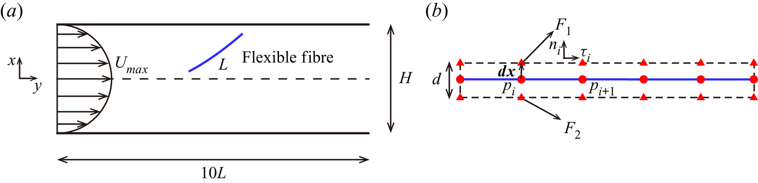
The motion of a neutrally buoyant flap inside planar Poiseuille flow is illustrated in figure 1(a), where  $H$ denotes the channel width,
 $L$ is the contour length of flap and
 $U_{max}$ is maximum velocity in the Poiseuille flow without a flap. The incompressible Navier–Stokes equations that govern the flow are
 \begin{gather} \boldsymbol{\nabla}\boldsymbol{\cdot}\boldsymbol{v} = 0, \end{gather}
 \begin{gather}\frac{\partial \boldsymbol{v}}{\partial t}+\boldsymbol{v} \boldsymbol{\cdot}\boldsymbol{\nabla}\boldsymbol{v}={-}\frac{1}{\rho} \boldsymbol{\nabla} p + \frac{\mu}{\rho}\nabla^2\boldsymbol{v}+\boldsymbol{f}, \end{gather}
where  $\rho$ is the fluid density,
 $\boldsymbol {v}$ is the velocity,
 $p$ is the pressure,
 $\mu$ is the dynamic viscosity of the fluid and
 $\boldsymbol {f}$ is the body force term. The dynamics of a fine flexible flap can be described by the Euler–Bernoulli beam equation,
 \begin{align} \rho_s h \frac{\partial^2 \boldsymbol{X}}{\partial t^2}=\frac{\partial}{\partial s}\left[Eh\left(1-\left(\frac{\partial \boldsymbol{X}}{\partial s}\boldsymbol{\cdot}\frac{\partial\boldsymbol{X}}{\partial s}\right)^{{-}1/2} \right)\frac{\partial \boldsymbol{X}}{\partial s}-\frac{\partial}{\partial s} \left(EI\frac{\partial ^2\boldsymbol{X}}{\partial s^2}\right)\right]+\boldsymbol{F}_{L}+\boldsymbol{F}_{c}+\boldsymbol{F}_{g}, \end{align}
where  $\rho _{s}$ is the density of the flap,
 $h$ is the thickness,
 $\boldsymbol {X}$ is the position of the flap,
 $s$ is the Lagrangian coordinate along the flap. Here
 $\boldsymbol {F}_{L}$ is the Lagrangian force exerted on the flap by the surrounding fluid, and
 $\boldsymbol {F}_{c}$ is the repulsive force to avoid contact and overlap between flap elements and the wall. Here
 $\boldsymbol {F}_{g}=\rho _s h \boldsymbol {g}$ is the gravity force, and
 $g=|\boldsymbol {g}|$ is the acceleration of gravity. Since we study a neutrally buoyant flap, gravity is not considered, i.e.
 $\boldsymbol {F}_{g}=0$. Here
 $Eh$ and
 $EI$ are the stretching and bending stiffnesses, respectively.
(a) Schematic diagram of a free flap in Poiseuille flow. (b) Zoom-in view of the flap. The red triangles and circles represent the ghost points and the Lagrangian points, respectively. Here  $F_1$ and
 $F_2$ are the fluid force on two ghost points;
 $\boldsymbol {n}_{i}$ and
 $\boldsymbol {\tau }_{i}$ are local normal and tangential unit vectors, respectively;
 $\boldsymbol {{d} x}$ denotes the position vector and
 $|\boldsymbol {{d} x}|=d/2$, where
 $d$ is the thickness of the flap.

The boundary conditions of the flap at both ends are
 \begin{equation} 1-\left(\frac{\partial \boldsymbol{X}}{\partial s}\boldsymbol{\cdot}\frac{\partial \boldsymbol{X}}{\partial s}\right)^{{-}1/2}=0,\quad \frac{\partial ^2\boldsymbol{X}}{\partial s^2}=(0,0),\quad \frac{\partial ^3\boldsymbol{X}}{\partial s^3}=(0,0), \end{equation}
which mean no tension force, no bending moment and no shearing force, respectively.
The reference quantities density  $\rho$, velocity
 $U_{max}$ and length
 $L$ are chosen to normalize the above formulations. The characteristic time and force are
 $T_{ref}=L/U_{max}$ and
 $F_{ref}=\frac {1}{2} \rho U_{max}^2L$, respectively. The key non-dimensional parameters are listed as follows: the Reynolds number
 $\textit {Re} =\rho U_{max} L/\mu$; the bending stiffness
 $K=EI/\rho U_{max}^2L^3$; the stretching stiffness
 $S=Eh/\rho U_{max}^2L$; and the channel confinement ratio
 $W=H/L$.
3. Numerical method and validation
3.1. Numerical method
3.1.1. Lattice Boltzmann method
The flow-governing equations (2.1) and (2.2) are solved by the lattice Boltzmann method (Chen & Doolen Reference Chen and Doolen1998). The discrete lattice Boltzmann equation with the Bhatnagar–Gross–Krook (BGK) collision model is
 \begin{equation} f_{i}(\boldsymbol{x}+\boldsymbol{e}_{i}\Delta t,t+\Delta t) - f_{i}(\boldsymbol{x},t) ={-}\frac{1}{\tau}\left [ f_{i}(\boldsymbol{x},t) - f_{i}^{eq}(\boldsymbol{x},t) \right ]+ \Delta t F_{i} , \end{equation}
where  $f_{i}(\boldsymbol {x},t)$ is the distribution function for particles with velocity
 $\boldsymbol {e}_{i}$ at position
 $\boldsymbol {x}$ and time
 $t$. Here
 $\tau$ is the non-dimensional relaxation time related to the fluid viscosity,
 $\nu =c_{s}^{2}(\tau -0.5)\Delta t$, where
 $\Delta t$ is the time step. The equilibrium distribution function
 $f_{i}^{eq}(\boldsymbol {x},t)$ and the forcing term
 ${F}_{i}$ (Guo, Zheng & Shi Reference Guo, Zheng and Shi2002) are defined as
 \begin{gather} f_{i}^{eq}=w_{i}\rho \left [ 1+ \frac{\boldsymbol{e}_{i}\boldsymbol{\cdot} \boldsymbol{v}}{c_{s}^{2}} + \frac{\left ( \boldsymbol{e}_{i}\boldsymbol{\cdot} \boldsymbol{v} \right )^{2}}{2c_{s}^{4}}-\frac{ \boldsymbol{v} ^{2}}{2c_{s}^{2}}\right ], \end{gather}
 \begin{gather}F_{i}=\left( 1-\frac{1}{2\tau} \right)w_{i} \left [ \frac{\boldsymbol{e}_i- \boldsymbol{v}}{c_{s}^{2}}+ \frac{\boldsymbol{e}_i\boldsymbol{\cdot} \boldsymbol{v}}{c_{s}^{4}}\boldsymbol{e}_i \right ]\boldsymbol{\cdot} \boldsymbol{f}, \end{gather}
where  $c_{s}=c/\sqrt {3}$ is the speed of sound,
 $c=\Delta x /\Delta t$ is the lattice speed,
 $\Delta x$ is the grid spacing of the uniform mesh,
 $\boldsymbol {f}$ is the body force,
 $w_{i}$ is the weighting factor, for the D2Q9 model,
 $w_{i }= 4/9$ (
 $i = 0$),
 $w_{i }= 1/9$ (
 $i = 1,2,3,4$),
 $w_{i}=1/36$ (
 $i = 5,6,7,8$). The 2-D D2Q9 velocity model is
 \begin{equation} \boldsymbol{e}_{i} = c \boldsymbol{\cdot} \left[ {{\begin{array}{ccccccccc} 0 & 1 & 0 & {-1} & 0 & 1 & {-1} & {-1} & 1 \\ 0 & 0 & 1 & 0 & {-1} & 1 & 1 & {-1} & {-1} \end{array}}}\right]. \end{equation}
The macroscopic velocity  $\boldsymbol {v}$, mass density
 $\rho$ and pressure p can be obtained through
 \begin{equation} \rho =\sum_{i}f_{i} , \quad \rho \boldsymbol{v}=\sum_{i}\boldsymbol{e}_i\,f_{i}+\frac{1}{2}\ \boldsymbol{f}\Delta t, \quad p=c_{s}^{2}\rho. \end{equation}
3.1.2. Immersed boundary method
The fluid–solid interaction is coupled through the immersed boundary (IB) method (Peskin Reference Peskin2002; Mittal & Iaccarino Reference Mittal and Iaccarino2005). The Lagrangian force  $\boldsymbol {F}_{L}$ between the fluid and structure can be calculated by the penalty scheme (Goldstein, Handler & Sirovich Reference Goldstein, Handler and Sirovich1993; Huang, Chang & Sung Reference Huang, Chang and Sung2011),
 \begin{equation} \boldsymbol{F}_{L}=\alpha\int^t_0[\boldsymbol{V}_f(s,t^\prime)-\boldsymbol{V}_s(s,t^\prime)]\, \mathrm{d}t^\prime +\beta[\boldsymbol{V}_f(s,t)-\boldsymbol{V}_s(s,t)], \end{equation}
where  $\alpha$ and
 $\beta$ are parameters which are selected based on the previous studies (Huang, Wei & Lu Reference Huang, Wei and Lu2018; Peng, Huang & Lu Reference Peng, Huang and Lu2018; Zhang, Huang & Lu Reference Zhang, Huang and Lu2020),
 $\boldsymbol {V}_s=\partial \boldsymbol {X}/\partial t$ is the velocity of the flap at the Lagrangian points (solid points) and
 $\boldsymbol {V}_f$ is the fluid velocity at the position
 $\boldsymbol {X}$ obtained by interpolation,
 \begin{equation} \boldsymbol{V}_f(s,t)=\int_{\varOmega}\boldsymbol{v}(\boldsymbol{x},t)\delta(\boldsymbol{x}-\boldsymbol{X}(s,t))\,{\rm d}\kern0.06em \boldsymbol{x}, \end{equation}
where the subscript  $\varOmega$ denotes the whole computational domain.
Then the Dirac delta function is used to transform the Lagrangian force  $\boldsymbol {F}_{L}$ to the body force
 $\boldsymbol {f}$ on the Eulerian points (fluid points),
 \begin{equation} \boldsymbol{f}(\boldsymbol{x},t)={-}\int_{\varGamma}\boldsymbol{F}_{L}(s,t)\delta(\boldsymbol{x}-\boldsymbol{X}(s,t))\,{\rm d}s, \end{equation}
where the subscript  $\varGamma$ means the integral is along the flexible flap.
3.1.3. Solution of flap equations
To evaluate the moment exerted by the surrounding fluid, two ghost points at a small radial distance around each of the Lagrangian points (Banaei, Rosti & Brandt Reference Banaei, Rosti and Brandt2020) is considered,  $\boldsymbol {{d} x}$ denotes the position vector and
 $|\boldsymbol {{d} x}|=d/2$, where
 $d$ is the thickness of the flap (see figure 1b). The forces
 $\boldsymbol {F}_1$ and
 $\boldsymbol {F}_2$ on the ghost points are calculated by the IB method. Then the moment on the elements
 $s_i$ can be obtained through
 \begin{equation} \boldsymbol{M}_{i}= \boldsymbol{{d} x} \times \boldsymbol{F}_1 -\boldsymbol{{d} x} \times \boldsymbol{F}_2. \end{equation}
The moment can be converted to a pure moment acting on the Lagrangian points  $p_i$ and
 $p_{i+1}$ to correct the Lagrangian force
 $\boldsymbol {F}_{L}$. Further, in order to avoid non-physical overlap, a repulsive force
 $\boldsymbol {f}$ (Banaei et al. Reference Banaei, Rosti and Brandt2020) is introduced when the gap between the flap and the wall, or the flap elements
 $r$, is less than a specified threshold
 $r_0$,
 \begin{gather} \phi (r)=D_{e}[\exp({2a(r_0-r)})-2\exp({a(r_0-r)})], \end{gather}
 \begin{gather}\boldsymbol{f}={-} \frac{\mathrm{d} \phi }{\mathrm{d} r}\boldsymbol{d}_{ij}, \end{gather}
where the parameter  $D_{e}$ governs the interaction strength,
 $a$ is a scaling factor,
 $r_0$ is the cutoff force distance,
 $\boldsymbol {d}_{ij}$ is the unit vector connecting the contact points.
The total repulsive force on the  $i$th element is obtained by
 \begin{equation} \boldsymbol{F}_{ci}=\sum_{j\neq i}^{N}\ \boldsymbol{f}, \end{equation}
where  $N$ is the number of the elements closer than the threshold
 $r_0$. Here
 $r_0=3d$ is specified. Parameter studies show that the results are not sensitive to the strength of the repulsive force.
The forces  $\boldsymbol {F}_{L}$ and
 $\boldsymbol {F}_c$ are applied to (2.3). Then, (2.3) is solved by the nonlinear finite element method with the large-displacement deformation problem handled by a corotational scheme; a detailed description of this method can be found in Doyle (Reference Doyle2013).
3.2. Validation
3.2.1. Wall-mounted deformable filaments in oscillatory flow
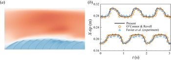
We consider a row of 10 wall-mounted flexible filaments inside a channel with a flow driven by an oscillatory pressure gradient and compare our results with those obtained from experiments (Favier et al. Reference Favier, Li, Kamps, Revell, O'Connor and Brücker2017) and computations (O'Connor & Revell Reference O'Connor and Revell2019). An instantaneous visualization of the row of filaments in the channel is shown in figure 2(a). In our case, the sinusoidally varying pressure gradient is  ${\rm d}p/{{\rm d}\kern0.06em x} = A\sin (2{\rm \pi} ft)$, where
 $A = 4549.13\,{\rm Pa}\ {\rm m}^{-1}$,
 $f=1.0$ Hz. The Reynolds number is defined as
 $Re = U_{max}L/\nu = 120$, where
 $U_{max}$ is the maximum flow velocity without filaments. The computational domain size is
 $22L \times 3L$. The periodic boundary condition is applied to the left-hand and the right-hand boundaries. And non-slip boundary condition is applied to the upper and lower boundaries. The horizontal gap spacing between the feet of two neighbouring filaments is
 $0.5L$. The streamwise tip positions for the first (the lower curves) and the 10th filaments (the upper curves) are shown in figure 2(b). They also compared with the experiment data in Favier et al. (Reference Favier, Li, Kamps, Revell, O'Connor and Brücker2017) and the simulation results of O'Connor & Revell (Reference O'Connor and Revell2019). It is seen that our simulation results agree well with both the experimental and numerical results. The slight deviation between simulation and experiment may be attributed to the approximation of the experimental parameters and the 3-D effect.
(a) Instantaneous visualization of the row of filaments in the channel. The streamwise velocity contours are also shown. (b) Streamwise tip positions for the first (the lower curves) and the 10th (the upper curves) filaments compared with Favier et al. (Reference Favier, Li, Kamps, Revell, O'Connor and Brücker2017) and O'Connor & Revell (Reference O'Connor and Revell2019).

3.2.2. A flexible flapping plate with  $Re = 150$

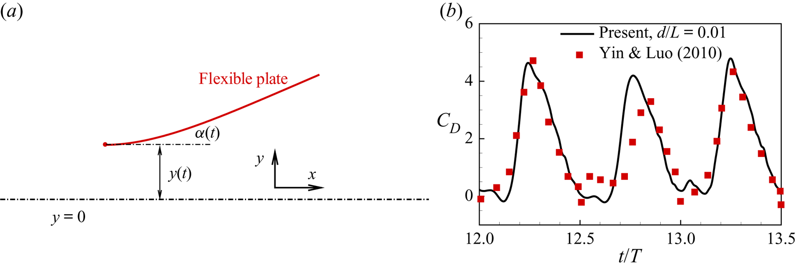
A flexible flapping plate is considered, as shown in figure 3(a). The forced motions of the leading edge are prescribed by
 \begin{equation} x(t)=x_0, \quad y(t)=A \cos (2 {\rm \pi}f t), \quad \alpha(t) = \alpha_0 \sin(2 {\rm \pi}f t), \end{equation}
where  $x_0$ is the initial horizontal location of the leading edge,
 $y(t)$ and
 $\alpha (t)$ are translational and rotational motions, respectively,
 $A$ and
 $f$ are the flapping amplitude and frequency, respectively,
 $\alpha _0$ is the rotational amplitude. In this case, only the leading edge of the plate is restricted with the prescribed motions and the remainder of the plate can move freely. A typical case with
 $Re = U_{ref} L / \nu = 150$, where
 $U_{ref}=2{\rm \pi} Af$. The other key parameters are
 $A/L = 1.25$,
 $\alpha _0=0$,
 $K=0.2$,
 $M=\rho _s h/\rho L=1$,
 $S=1000$ and the plate thickness
 $d=0.01L$. The non-dimensional computational domain size is
 $[-15,25] \times [-15,15]$ and the grid spacing is
 $\Delta x=0.01L$. The drag coefficient
 $C_D={F_y}/(({\rho {U_{ref}}^2 L})/2)$, where
 $F_y$ is the drag force in the vertical direction. Both our result and that of Yin & Luo (Reference Yin and Luo2010) are shown in figure 3(b). It is seen that our result agrees well with Yin & Luo (Reference Yin and Luo2010).
(a) Sketch of a model for a flapping plate. (b) Drag coefficient ( $C_D$) of the flexible plate as a function of time. Corresponding result of Yin & Luo (Reference Yin and Luo2010) is also presented.

3.2.3. A single rigid flap in a shear flow
The motion of an individual flap in a shear flow is studied. The non-dimensionalized computational dimensions are  $[-4,4]\times [-5,5]$ with space step
 $\Delta x /L_{ref}=0.0625$, time step
 $\Delta t /T_{ref}=0.00125$, and the flap is discretized into 32 elements with 33 Lagrangian points. A rigid flap with
 $K=10^2$ is considered. The flow is close to the Stokes flow since
 $\textit {Re}$ is very small in the simulation (
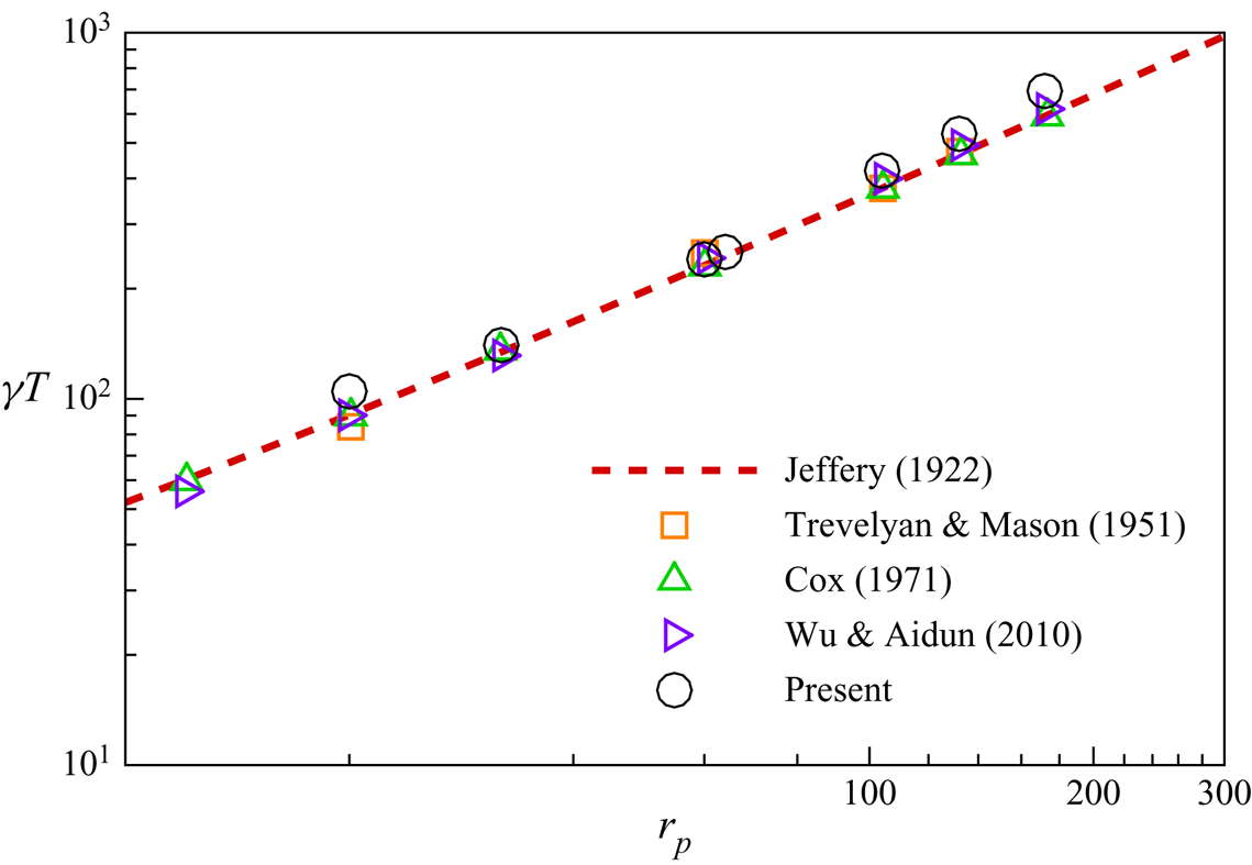
 $\textit {Re}=0.1$). Figure 4 shows the normalized rotational period
 $\gamma T$ as a function of the flap aspect ratio
 $r_{p}$. Our simulation result agrees well with the analytical and numerical results in the literature (Jeffery Reference Jeffery1922; Trevelyan & Mason Reference Trevelyan and Mason1951; Cox Reference Cox1971; Wu & Aidun Reference Wu and Aidun2010).
Rotational period  $\gamma T$ as a function of the aspect ratio
 $r_{p}$ in shear flow compared with Jeffery (Reference Jeffery1922), Trevelyan & Mason (Reference Trevelyan and Mason1951), Cox (Reference Cox1971) and Wu & Aidun (Reference Wu and Aidun2010).

3.2.4. Grid convergence validation
A case of a flexible flap in a planar Poiseuille flow is simulated. The non-dimensional computational domain size is  $[-2, 2] \times [-2, 2]$, i.e. the channel width is
 $H=4L$. The planar Poiseuille flow is driven by a constant body force, and periodic boundary conditions are applied at the left-hand and right-hand boundaries. The other key parameters are
 $Re=30$ and
 $K=10^{-3}$. The flap with fixed aspect ratio
 $r_p=64$ is initially aligned with the flow and released from
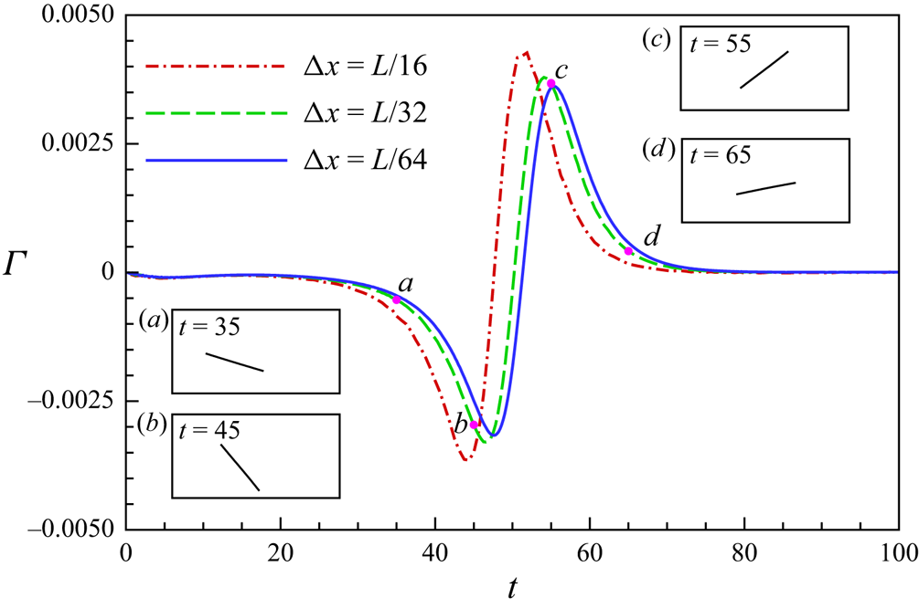
 $y_0=-1$. Three cases with different grid spacing
 $\Delta x=\frac {1}{16}L$,
 $\frac {1}{32}L$ and
 $\frac {1}{64}L$ are simulated. The normalized torques
 $\varGamma$ experienced by the fibre as functions of non-dimensional time
 $t$ are shown in figure 5. It is seen that although the evolution of
 $\varGamma$ in the case
 $\Delta x=\frac {1}{16}L$ has a significant discrepancy with those in the cases of
 $\Delta x=\frac {1}{32}L$,
 $\frac {1}{64}$,
 $\varGamma$ in the case
 $\Delta x=\frac {1}{32}L$ is very close to that in the case
 $\Delta x=\frac {1}{64} L$. The discrepancy between the peaks is only approximately 2.7 %. Therefore,
 $\Delta x=\frac {1}{32}L$ seems sufficient to get accurate results, i.e. 32 Lagrangian grids for a flap is enough.
The normalized torques  $\varGamma$ as functions of non-dimensional time
 $t$. The time and torque are normalized by
 $L/U_{max}$ and
 $\varGamma _{ref}= 1/2 \rho U_{max}^2 L^2$, respectively.

4. Results and discussion
In our study, the flap is inextensible with a sufficient large stretching stiffness, i.e.  $S=10^4$. We study the effect of the bending stiffness
 $K$, Reynolds number
 $\textit {Re}$ and channel confinement ratio
 $W$ on the flap deformation, tumbling and cross-stream migration. The parameter ranges in our study are
 $K\in [10^{-4}, 10^2]$,
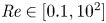 $\textit {Re} \in [0.1,10^2]$ and
 $W\in [1,4]$.
The planar Poiseuille flow is driven by a constant body force and periodic boundary conditions are applied at the inlet and outlet. Convergence tests for different computational domains show that the computation domain size  $L_x =[-5,5]$ is large enough to eliminate the effect of the periodic boundary condition. The flap with fixed aspect ratio
 $r_p=L/d=64$ is initially aligned with the flow and placed slightly offset from the channel centre, e.g.
 $y_{0}=-0.02L$.
4.1. Motion modes and phase diagram
Under different circumstances, the flap may undergo different configurations which depends on the interplay of flow drag (viscous force and pressure), fluid inertia and flap elastic restoring force. Since the Poiseuille flow is also a shear flow with non-uniform shear rate, the movement would be somewhat similar to those in the Couette flow (Forgacs & Mason Reference Forgacs and Mason1959). On the other hand, some new motion modes that have never been found in the Couette flow are revealed here, e.g. the swinging mode.
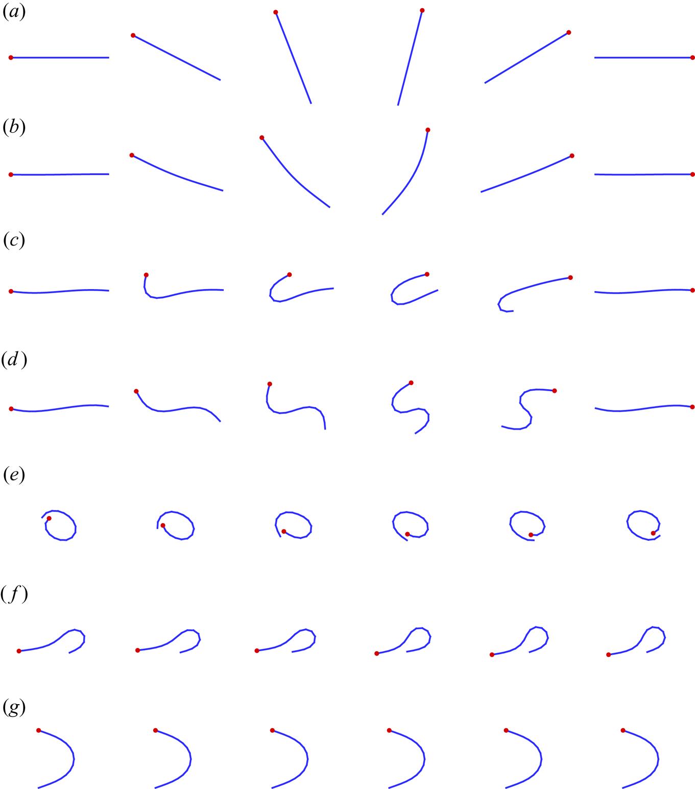
Typical periodic morphological evolutions of the flap during a half-period are shown in figure 6. They correspond to different motion modes. As shown in figure 6(a), the flap behaves like a rigid rod tumbling around its centre of mass (COM). It is referred to as rigid motion. The springy motion, which is also called C buckling, is shown in figure 6(b). In this mode, during its tumbling, the flap would bend a little bit, but when it is almost horizontal, it becomes straight again. The U-turn motion is shown in figure 6(c), the flap behaves like a tank-treading rotation. For the S-turn motion (see figure 6d), the two ends curl in opposite directions. It is noticed that the S-turn motion rarely occurs in our simulations. The U-turn motion and S-turn motion are also referred to as single-end and double-end snake turns, respectively, in Forgacs & Mason (Reference Forgacs and Mason1959). Further, we observed that a more flexible flap appears to have more complex motion (see figure 6e,f). For a narrow channel, a stable parabolic configuration appears (see figure 6g), the flap keeps this shape moving along the flow. Table 1 shows the specific parameters for each of the motion modes in figure 6.
Typical periodic morphological evolutions of the flap during a half-period: (a) rigid motion; (b) springy motion; (c) U-turn motion; (d) S-turn motion; (e,f) complex motions; (g) stable mode. The red point denotes the head of the flap, and the fluid flows from left to right.

Parameters for the motion modes in figure 6. In all cases  $r_p=64$ except (d), in which
 $r_p=16$.

To quantify the characteristics of the above motion modes, the criterion based on the gyration tensor (Liu et al. Reference Liu, Chakrabarti, Saintillan, Lindner and Du Roure2018) is adopted. The gyration tensor is defined as
 \begin{equation} G_{\xi \eta }=\sum_{i=1}^{N}(r_\xi(i,t)-\bar{r}_\xi(t))(r_\eta (i,t)-\bar{r}_\eta(t))/N, \end{equation}
where  $N$ denotes the total number of Lagrangian points in the flap,
 $r_\xi (i,t)$ and
 $\bar {r}_\xi (t)$ denote the instantaneous position of
 $p_i$ and the COM of the flap, respectively, and the subscripts
 $\xi$,
 $\eta$ denote
 $x$ or
 $y$. Shape anisotropy
 $\omega$ is defined as
 \begin{equation} \omega=1-4\lambda_1\lambda_2/(\lambda_1+\lambda_2)^2, \end{equation}
where  $\lambda _1$,
 $\lambda _2$ are the eigenvalues of the gyration tensor. These two eigenvalues as the semiaxes naturally lead to an ellipse. Here
 $\omega \approx 0$, i.e.
 $\lambda _1\approx \lambda _2$, denotes a nearly symmetric configuration, while
 $\omega \approx 1$, i.e.
 $\lambda _1\gg \lambda _2$, denotes a nearly straight configuration. The mean rotation angle
 $\alpha$ is defined as the angle between the flow direction and the mean flap orientation, which is represented by the angle between the
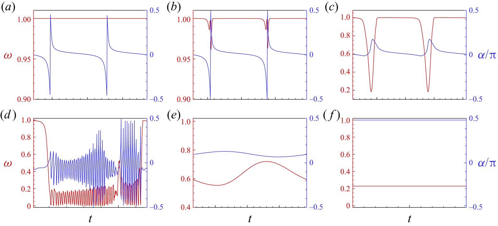
 $x$ axis and the eigenvector corresponding to the largest eigenvalue of the gyration tensor. Figure 7 shows the evolutions of these two parameters in a period for the motion modes in figure 6. For the rigid motion, the flap keeps straight with
 $\omega \approx 1$, and
 $\alpha$ changes from
 $-{\rm \pi} /2$ to
 ${\rm \pi} /2$. For the springy motion, flap buckling occurs, thus
 $\omega$ has a significant oscillation when the flap is perpendicular to the flow direction (
 $\alpha \approx -{\rm \pi} /2$ or
 ${\rm \pi} /2$). The critical
 $\omega$ between the rigid and springy modes is set to
 $\omega =0.999$. For the U-turn motion,
 $\alpha$ fluctuates with a small amplitude, which differs from the above two modes. For the S-turn motion, since we cannot distinguish this mode by the evolutions of
 $\omega$ and
 $\alpha$, it has to be identified through shape evolution. For the rotational complex motion (figure 6e), the variations of
 $\omega$ and
 $\alpha$ are complicated (see figure 7d). For the steady complex motion (figure 6f),
 $\alpha$ is almost a constant (see figure 7e) because it almost always keeps a complex curved shape. For the stable mode, both
 $\omega$ and
 $\alpha$ are constant (see figure 7f).
The time evolution of  $\omega$ and
 $\alpha$ for (a) rigid motion, (b) springy motion, (c) U-turn motion, (d,e) complex motions, (f) stable mode. The cases correspond to those in figure 6.

A large number of cases with different  $W$,
 $\textit {Re}$ and
 $K$ were simulated. Besides, different initial orientations and positions were tried. Based on limited results, it is found that the final motion mode of the flap does not depend on the initial conditions. The final motion mode distributions in the
 $K$–
 $\textit {Re}$ plane for
 $W=4$,
 $W=2$ and
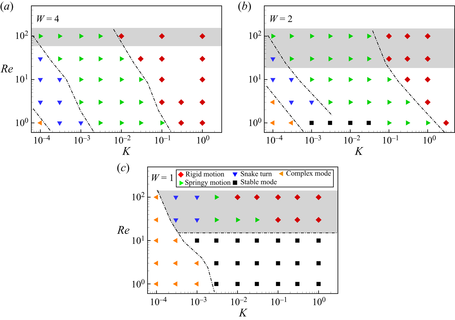
 $W=1$ are shown in figure 8. For
 $W=4$, the channel is wide enough and the wall effect is minor. When bending stiffness
 $K$ is relatively large, the flap adopts rigid motion. As
 $K$ decreases, the flap becomes more flexible, and the springy motion appears. As
 $K$ further decreases, the snake turn occurs. It is also seen that as
 $\textit {Re}$ increases, the borders between any two neighbouring modes all move leftward. It seems that the fluid inertia delays the appearance of the modes with more severe deformation. In other words, the fluid inertia tends to straighten the flap. It is noticed that when
 $\textit {Re}$ exceeds a threshold, e.g.
 $\textit {Re}\geqslant 65$ for cases of
 $W=4$, the flap swings around the COM of the flap instead of tumbling.
Phase diagrams for the cases of (a)  $W=4$, (b)
 $W=2$, (c)
 $W=1$. Each point in the phase diagram denotes a simulated case. The grey shading indicates the swinging mode.

For  $W=2$, the motion of the flap will be affected significantly by the wall. As shown in figure 8(b) that overall the mode distribution is similar to that of
 $W=4$ except for two differences. One is that the borders or the critical values of
 $K$ between any two neighbouring modes all slightly move rightward. The other is the appearance of the stable mode in the bottom of the plane. The possible reason is that due to the confinement effect of the walls, the flap is more likely to bend.
For  $W=1$, the movement of the flap is severely constrained by the walls. The flap mostly adopts the stable mode (
 $\textit {Re}<10$ and
 $K>10^{-3}$). For relatively large
 $\textit {Re}$ (e.g.
 $\textit {Re}=30$), as
 $K$ decreases, the rigid motion, springy motion and snake turn appear in sequence, and in all cases, the flap swings and is unable to tumble. When the flap is sufficiently flexible, it adopts a complex mode. The rigid swinging mode is similar to the oscillation observed in Nagel et al. (Reference Nagel, Brun, Berthet, Lindner, Gallaire and Duprat2018).
4.2. Effects of Reynolds number $\textit {Re}$

In this section, we mainly discuss the effect of  $\textit {Re}$ on the cross-stream migration and tumbling of flaps. First, the effect of
 $\textit {Re}$ on rigid flaps is discussed with
 $K=10^2$. The flap tumbles or swings like a rigid rod at small and large
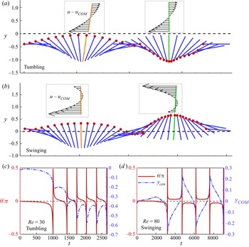
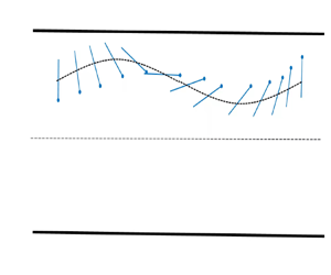
 $Re$, respectively. The sketches of the successive position and orientation of the flap in the tumbling or swinging modes are shown in figure 9(a,b). It is seen that the flap tumbles clockwise on one side of the centreline. The relative velocity profiles at two typical instants with respect to the COM of the flap can be found in the insets, which are similar to those in pure Couette flow. Therefore, the tumbling behaviour looks like that in Couette flow. However, in the swinging mode (see figure 9b), the COM of the flap fluctuates up and down across the centreline. Besides, from the two instantaneous velocity profiles (see the insets), we can imagine that the flap may experience clockwise and anticlockwise torques alternately in one period. Therefore, the flap would swing.
(a,b) Schematic diagram for the rigid mode (the axes scales are different). The insets are the relative velocity profiles with respect to the COM of the flap in the absent of flap. The orientation angle  $\theta$ and the lateral location
 $y_{COM}$ of the COM of the flap as functions of
 $t$ for typical cases: (c)
 $\textit {Re}=30$,
 $K=10^2$; (d)
 $\textit {Re}=80$,
 $K=10^2$.

To quantify the orientation of the flap, the angle between the end-to-end vector of the flap and the flow direction  $\theta$ is introduced here. The typical evolution of the lateral location of the COM of the flap
 $y_{COM}$ and
 $\theta$ are shown in figure 9(c,d). It is seen from figure 9(c) that initially the flap would migrate laterally and then fluctuate up and down around an equilibrium location
 $y_{COM}\approx -0.5$ periodically. At a larger
 $\textit {Re}$, e.g.
 $\textit {Re}=80$, the flap adopts the swinging mode (see figure 9d). In this mode, the flap fluctuates up and down around the equilibrium location
 $y_{COM}=0$, and it is not able to approach the horizontal orientation, i.e.
 $\theta =0$. We also observed that the flap's instantaneous velocity along the flow is only slightly slower than the ambient Poiseuille flow at the same lateral location (Słowicka et al. Reference Słowicka, Ekiel-Jeżewska, Sadlej and Wajnryb2012). Besides, neither the terminal equilibrium lateral location nor the final motion mode depend on the initial lateral position.
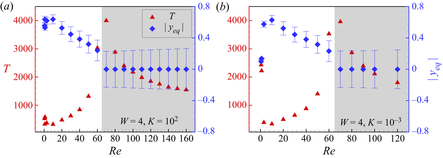
Next, we would like to discuss the inertial effect on the period of tumbling or swinging and the lateral equilibrium location  $|y_{eq}|$. The period
 $T$ and
 $|y_{eq}|$ as functions of
 $\textit {Re}$ for a typical rigid flap (
 $K=10^2$) and a flexible flap (
 $K=10^{-3}$) are shown in figure 10(a,b), respectively. The time-averaged lateral location of the COM of the flap
 $|y_{eq}|$ is defined as
 $|y_{eq}|=1/nT\int _{0}^{nT}y_{COM}\,{\rm d}t$. The error bar on
 $|y_{eq}|$ denotes the fluctuation of the lateral location during one period.
The period  $T$ and
 $|y_{eq}|$ as functions of
 $\textit {Re}$ for cases (a)
 $K=10^2$, (b)
 $K=10^{-3}$ at
 $W=4$.

For the case of  $W=4$,
 $K=10^2$ (see figure 10a), when
 $\textit {Re}\leqslant 60$, similar to the elliptical particle (Chen, Pan & Chang Reference Chen, Pan and Chang2012), as
 $\textit {Re}$ increases, the flap migrates away from the centreline of the channel and then approaches the centreline. The period is mainly related to the local shear rate, when
 $|y_{eq}|$ decreases, the local shear rate decreases and thereby the period increases. That is the variation trend of
 $T$ when
 $\textit {Re}\leqslant 60$. When
 $\textit {Re}\approx 65$, the flap no longer tumbles but stays tilted, moving along with the flow. When
 $\textit {Re}\geqslant 70$,
 $|y_{eq}|=0$, the flap adopts the swinging mode instead of the tumbling mode. With the increase of fluid inertia, the flap swings faster since
 $T$ decreases.
For a typical flexible flap (see figure 10b), the variation trends of  $y_{eq}$ and
 $T$ look similar to those in figure 10(a), but we should notice that under low
 $\textit {Re}$ (approximately
 $\textit {Re}<1$), the flap may adopt the U-turn mode, which leads to a larger period
 $T$.
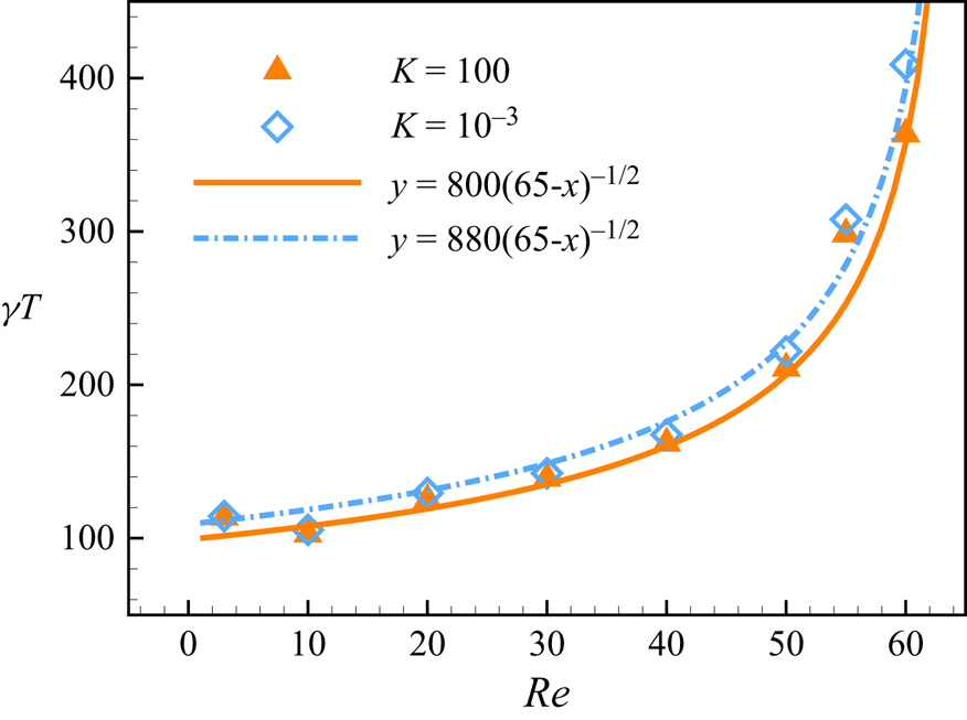
Ding & Aidun (Reference Ding and Aidun2000) predicted that the tumbling period of an ellipsoid particle is proportional to  $(\textit {Re}_{c} - \textit {Re})^{-1/2}$, and this scaling law is independent of the particle shape or the shear profile. In our simulation, the critical Reynolds number
 $\textit {Re}_c$ from the tumbling state to the stationary state is found at approximately
 $\textit {Re}_{c}=65$ at
 $W=4$. The local shear rate
 $\gamma$ at
 $y_{eq}$ is used to renormalize the period. The period of the flap is shown in figure 11. The fitting curve of our data is
 $\gamma T= C(\textit {Re}_{c}- \textit {Re})^{-1/2}$ with
 $Re_c=65$, and
 $C=800$ and
 $C=880$ for cases of
 $K=100$ and
 $K=10^{-3}$, respectively. It is seen that the tumbling period of a flap with different shape and flexibility as a function of
 $Re$ generally follows the scaling law for the ellipsoid, i.e.
 $\gamma T= C(\textit {Re}_{c}- \textit {Re})^{-1/2}$. However, it does not necessarily mean that neither shape nor flexibility plays a role in the tumbling period. For a more flexible fibre, the tumbling period is generally slightly larger at a specific
 $Re$ (we will discuss this in the next section).
The period  $\gamma T$ as a function of
 $Re$. The fitting curve is
 $\gamma T= C(Re_c- Re)^{-1/2}$ with
 $Re_c=65$ and
 $C=800$ and 880 for cases of
 $K=100$ and
 $K=10^{-3}$, respectively.

4.3. Effects of bending stiffness $K$

In this section,  $\textit {Re}$ and
 $W$ are fixed and we mainly discuss the effect of bending stiffness
 $K$ on flap motion. As the flexibility of the flap increases, the mode of the flap changes from rigid motion to springy motion and then to U-turn motion. To reveal the mechanism of different modes, we decompose the Lagrangian force
 $\boldsymbol {F}_{L}$ at the
 $i$th Lagrangian point, experienced by the flap into two parts: one is the normal force
 $\boldsymbol {F}_i^{n}$, in which the pressure component dominates; and the other is the tangential force
 $\boldsymbol {F}_i^{\tau }$, which mainly comes from the viscous effects. These forces at
 $i$th Lagrangian point are defined as (Peng et al. Reference Peng, Huang and Lu2018)
 \begin{gather} \boldsymbol{F}_i^{n}=(\boldsymbol{F}_{Li}\boldsymbol{\cdot}\boldsymbol{n}_i)\boldsymbol{n}_i=(F_{x,i}^{n},F_{y,i}^n), \end{gather}
 \begin{gather}\boldsymbol{F}_i^{\tau}=(\boldsymbol{F}_{Li}\boldsymbol{\cdot}\boldsymbol{\tau}_i)\boldsymbol{\tau}_i=(F_{x,i}^{\tau},F_{y,i}^{\tau}), \end{gather}
where  $\boldsymbol {n}_i$ and
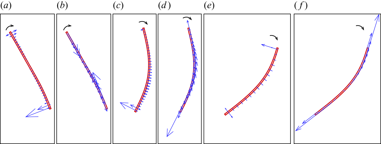
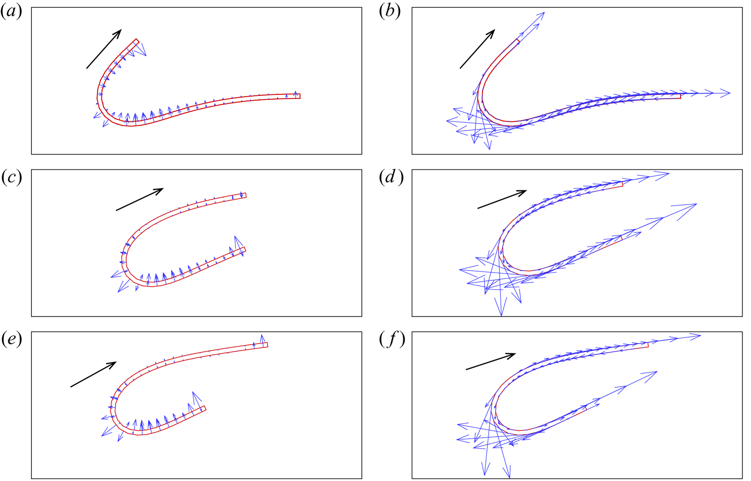
 $\boldsymbol {\tau }_i$ are the local unit normal and tangential vectors, respectively. Figures 12 and 13 show the examples of distribution of pressure and viscous forces on the flap, which adopt springy motion and U-turn motion, respectively. From figure 12(a,c,e), we can see that the tumbling of flap is mainly caused by the normal force generated by the pressure at the head and tail, and the magnitude of the normal force determines the rotation speed of the fibre. Before and after the flap passes through the orientation perpendicular to the streamline, the flap accelerates and decelerates, respectively. The viscous force (see figure 12b,d,f) mainly affects the shape of the flap, the flap is compressed and then stretched, so compared with rigid motion, the flap with a relatively small
 $K$ is deformed. The mechanism of U-turn motion is completely different, the normal force keeps the flap in a compact configuration, while the tangential force generated by the viscous force mainly results in a tank-treading movement (see figure 13).
The distribution of pressure and viscous forces on the flap which adopts springy motion at several typical moments. Panels (a,c,e) are the normal force generated by pressure, (b,d,f) are the tangential force generated by viscous forces. The control parameters are  $W=4,Re=30,K = 10^{-3}$.

The distribution of pressure and viscous forces on the flap which adopts U-turn motion at several typical moments. Panels (a,c,e) are the normal force generated by pressure, (b,d,f) are the tangential force generated by viscous forces. The control parameters are  $W=4,Re=30,K = 10^{-4}$.

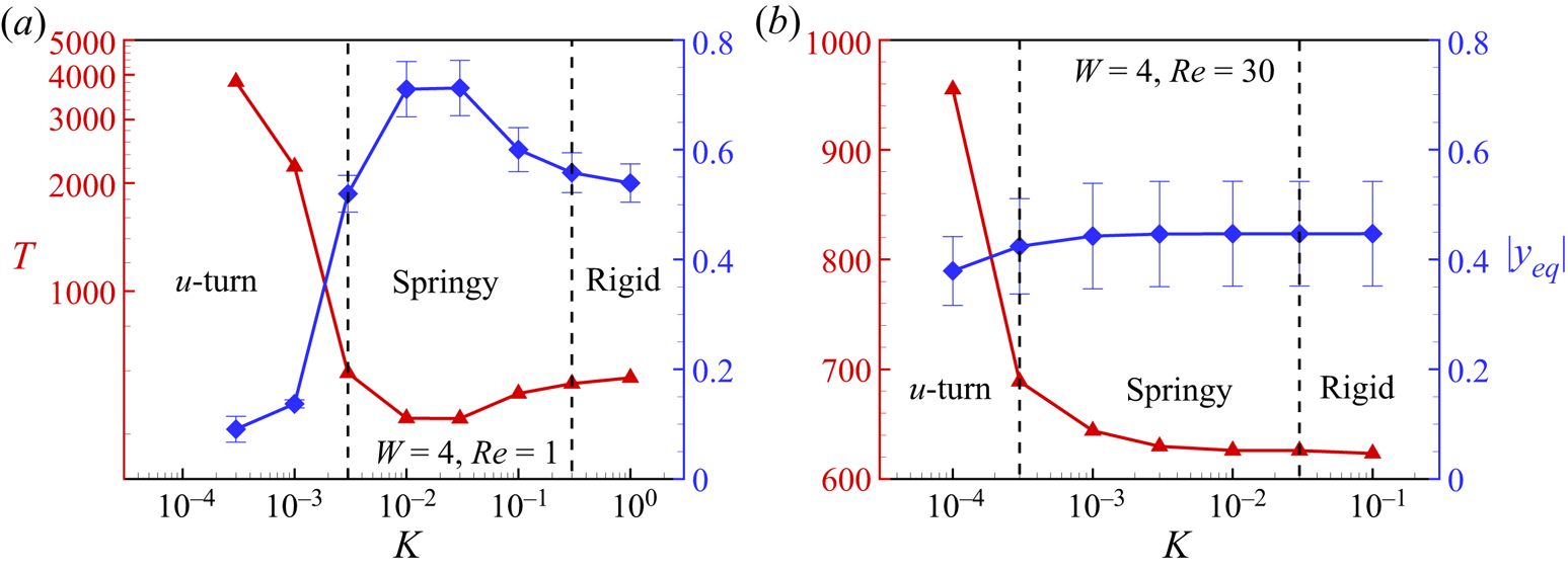
Next we study the influence of  $K$ on the period. Figure 14 shows
 $T$ and
 $|y_{eq}|$ as functions of
 $K$ at two typical
 $\textit {Re}$. From figure 14(a), we can see that the variation trend of equilibrium locations of flap at
 $Re = 1$ is close to that at
 $Re = 0$ (Słowicka et al. Reference Słowicka, Wajnryb and Ekiel-Jeżewska2013). Because the period of the tumbling mainly depends on the local shear rate, when the flap is closer to the centre of the channel, the local smaller shear rate induces a larger
 $T$. Hence the variation trends of
 $T$ and
 $|y_{eq}|$ are opposite. At
 $\textit {Re}=30$ (see figure 14b), the variation trends of
 $T$ and
 $|y_{eq}|$ are similar to those at
 $\textit {Re}=1$, but the flaps would be concentrated in the middle way between the centre of the channel and the wall due to fluid inertia.
Here  $T$ and
 $|y_{eq}|$ as functions of
 $K$ for cases: (a)
 $Re=1$ (log-scale); (b)
 $Re=30$ for
 $W=4$.

To reveal the effect of the deformation on the tumbling of the flap, the torques generated by  $\boldsymbol {F}_i^{n}$ and
 $\boldsymbol {F}_i^{\tau }$ with respect to the COM are calculated as
 \begin{gather} \varGamma_i^{n}=\boldsymbol{F}_i^{n}\boldsymbol{\cdot}\boldsymbol{r}={-}(y_i-y_{COM})F_{x,i}^{n} + (x_i-x_{COM})F_{y,i}^{n}, \end{gather}
 \begin{gather}\varGamma_i^{\tau}=\boldsymbol{F}_i^{\tau}\boldsymbol{\cdot}\boldsymbol{r}={-}(y_i-y_{COM})F_{x,i}^{\tau} + (x_i-x_{COM})F_{y,i}^{\tau}, \end{gather}
where  $(x_i,y_i)$ is the position of
 $i$th Lagrangian point, and
 $\boldsymbol {r}=(x_i-x_{COM},y_i-y_{COM})$ is the vector from the COM to the
 $i$th Lagrangian point. Anticlockwise torque is defined as positive.
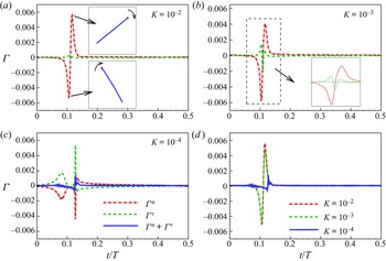
Figure 15 shows the time evolution of total  $\varGamma ^{n}$ and
 $\varGamma ^{\tau }$ (i.e.
 $\varGamma ^{n}=\sum _i\varGamma _i^{n}$ and
 $\varGamma ^{\tau }=\sum _i\varGamma _i^{\tau }$). It should be noted that in these cases the flaps rotate clockwise, and when
 $t/T=0$ the flaps are horizontal. As shown in figure 15(a), for relative rigid flaps,
 $\varGamma ^{n}$, i.e. pressure component, dominates the fluid–structure interactions, while the viscous effect basically does not affect the tumbling of flaps since
 $\varGamma ^{\tau }\approx 0$. When
 $\varGamma ^{n}$ is negative, it is in favour of the tumbling of the flap (see the lower inset). When
 $\varGamma ^{n}$ is positive, it hinders the tumbling (see the upper inset).
The time evolution of torque generated by fluid force during a half-period for typical cases (a)  $K=10^{-2}$, (b)
 $K=10^{-3}$, (c)
 $K=10^{-4}$. (d) The evolution of the total torque. In all cases, the other key parameters are
 $W=4$,
 $Re=30$. Anticlockwise torque is positive and in these cases the flap rotates clockwise.

As  $K$ decreases (see figure 15b), the viscous effect begins to make a significant contribution to the tumbling of the flap. It seems that the corresponding
 $\varGamma ^{\tau }$ is relevant to the deformation of the flap. When
 $\varGamma ^{n}$ reaches a valley it is favourable for tumbling, but at the moment
 $\varGamma ^{\tau }$ reaches a significant peak and
 $\varGamma ^{\tau }>0$ and it hinders the tumbling. This unfavourable contribution of
 $\varGamma ^{\tau }$ becomes more significant as
 $K$ decreases (see figure 15c,d). For the extremely flexible flaps that adopted a U-turn motion,
 $\varGamma ^{n}$ is almost counteracted by
 $\varGamma ^{\tau }$ (see figure 15c). From figure 15(d), we can see that the total torque, i.e.
 $\varGamma ^{n}+\varGamma ^{\tau }$, decreases with decreasing
 $K$. Therefore, it is expected that the rotational period would increase as
 $K$ decreases.
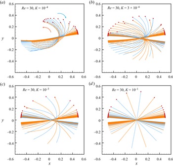
As mentioned above, at a relatively high  $\textit {Re}$, the COM of the flap fluctuates up and down near the centre of the channel, and meanwhile the flap swings around the COM due to the alternative positive and negative torques in one period. Figure 16 shows examples of instantaneous configurations in one period in the centroid coordinate system. Table 2 shows the period
 $T$ and the swinging amplitude
 $\Delta \theta$ as functions of
 $K$. The swinging amplitude
 $\Delta \theta$ is defined as the range of
 $\theta$. From the table, we can see that
 $\Delta \theta$ and
 $T$ decrease as
 $K$ decreases, and we observe a sharp decrease for the case of
 $K=10^{-4}$. The period is mainly related to the swinging amplitude.
Instantaneous configuration (full-body profile) in the centroid coordinate system in one period  $T$ for the cases of
 $W=2$,
 $Re=30$ with different
 $K$: (a)
 $K=10^{-4}$; (b)
 $K=3\times 10^{-4}$; (c)
 $K=10^{-3}$; (d)
 $K=10^{-1}$. The blue and yellow lines represent the clockwise and anticlockwise rotation, respectively, and the time interval between two adjacent lines is
 $5T_{ref}$.

The period  $T$ and the swinging amplitude
 $\Delta \theta /{\rm \pi}$ for cases of
 $W=2$,
 $\textit {Re}=30$ with different
 $K$; (a)–(d) are shown in figure 16.

4.4. Stable mode in a narrow channel
In this section, we discuss the stable mode in a narrow channel where the channel width is comparable to the length of the flap (e.g.  $W=1$). Due to the confinement of the wall, there is a high-pressure zone between the flap and the wall; that prevents the flap from tumbling. The rigid flap would maintain an inclined configuration moving along with the flow, while for the flexible flap, it bends to a parabolic-like configuration. For a very flexible flap, e.g.
 $K=10^{-3}$, it becomes a non-symmetric one-end bending configuration (see figure 17d). For these configurations, the lateral location of the COM is approximately at the centreline of the channel. The parabolic-like configuration has been experimentally (see figure 1c in Steinhauser et al. (Reference Steinhauser, Köster and Pfohl2012)) and numerically (see figure 5c in Reddig & Stark (Reference Reddig and Stark2011)) observed for an individual semiflexible actin fibre, in their studies
 $W\approx 1.25$. Also Karnis, Goldsmith & Mason (Reference Karnis, Goldsmith and Mason1966) experimentally observed this configuration (see figure 10 in Karnis et al. (Reference Karnis, Goldsmith and Mason1966)) for a prolate ellipsoid particle with fixed aspect ratio
 $r_p=78$ in a tube Poiseuille flow. In their studies
 $W\approx 0.9$ and
 $K\approx 3\times 10^{-3}$ if we approximate the elastic modulus
 $E$ of the rubber according to our definition. Hence, our result is consistent with that in the literature.
Pressure contours for typical cases: (a)  $K=3\times 10^{-1}$; (b)
 $K=10^{-2}$; (c)
 $K=8\times 10^{-3}$; (d)
 $K=10^{-3}$ at
 $W=1, \textit {Re}=6$.

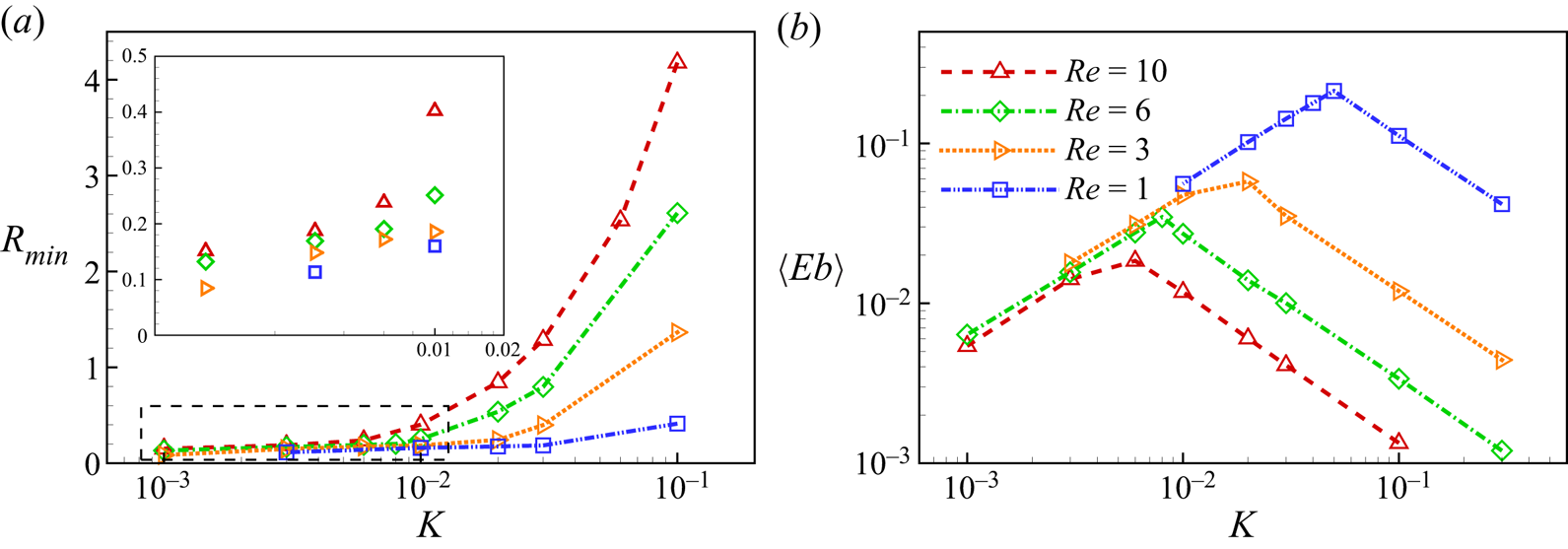
The amount of deformation of flaps can be quantified by minimum radius of curvature and time-averaged bending energy. For two adjacent elements, the radius of curvature is defined as (Lindström & Uesaka Reference Lindström and Uesaka2007)
 \begin{equation} R_i=\left | \frac{\frac{1}{2} (|\boldsymbol{l}_{i,i+1}|+|\boldsymbol{l}_{i-1,i}|)}{{\rm arccos}(\boldsymbol{l}_{i,i+1}\boldsymbol{\cdot} \boldsymbol{l}_{i-1,i})}\right |, \end{equation}
where  $\boldsymbol {l}_{i,i+1}$ is the vector from
 $p_{i}$ to
 $p_{i+1}$. The minimum radius of curvature is defined as
 $R_{min}=\min (R_i)$. It is noticed that, for an extreme flexible flap,
 $R_{min}\approx 0$ and for a rigid flap,
 $R_{min}\approx \infty$. Bending energy is defined as
 \begin{equation} \langle Eb\rangle=\frac{k}{2}\int_{0}^{L}\frac{\partial^2 \boldsymbol{x} }{\partial s^2}\boldsymbol{\cdot} \frac{\partial^2 \boldsymbol{x} }{\partial s^2}\,{\rm d}s. \end{equation}
The bending energy represents the global bending degree of the flap, while  $R_{min}$ represents the local bending degree of the flap. Figure 18(a,b) show
 $R_{min}$ and
 $\langle Eb\rangle$ as functions of
 $K$, respectively. As depicted in the figure,
 $R_{min}$ decreases monotonically as
 $K$ decreases. Obviously, the bending degree of the flap increases as the flap becomes more flexible. From figure 18(b), we observe that as
 $K$ decreases,
 $\langle Eb\rangle$ increases, and the flap gradually transits from a slight bending (see figure 17a) to a symmetrical configuration (see figure 17c). When
 $\langle Eb\rangle$ reaches a peak, the configuration of the flap is similar to the Poiseuille velocity profile. Then
 $\langle Eb\rangle$ decreases monotonically. This change is due to the transition from global bending to local bending (see figure 17d). In the global bending, the flap deforms as a whole while in the local bending, the two ends of the flap may deform independently, similar to the transition from springy motion to U-turn motion in a wide channel. Also seen from figure 18(a), at a lower
 $\textit {Re}$,
 $R_{min}$ is smaller and the local bending is more severe. Besides, for cases with lower
 $Re$, the local bending appears at a relatively larger
 $K$ (see from figure 18b). In other words, a higher
 $Re$ puts off the appearance of local bending to a smaller
 $K$ region. Hence, again we see that fluid inertia tends to straighten the configuration.
(a) The minimum radius of curvature  $R_{min}$ and (b) the average bending energy
 $\langle Eb\rangle$ as functions of
 $K$ at
 $W=1$.

5. Conclusion
In this study, the behaviours of an individual fine flexible flap ( $r_p=64$) in planar Poiseuille flow are numerically investigated. The effects of Reynolds number
 $\textit {Re}$, bending stiffness
 $K$ and channel confinement ratio
 $W$ are analysed.
When a flexible flap is immersed in a wide channel flow (e.g.  $W=4$), as
 $K$ decreases, we observe rigid motion, springy motion, snake turn and complex motion in sequence. As
 $\textit {Re}$ increases, the borders between two neighbouring modes in the
 $K$–
 $\textit {Re}$ plane move leftward, so it seems that the fluid inertia is able to resist the bending and tends to straighten the flap. When
 $\textit {Re}$ exceeds a threshold, the flap stays inclined instead of tumbling. As
 $\textit {Re}$ further increases, the flap adopts swinging mode.
Moreover, we observe that as  $\textit {Re}$ increases, the flap firstly migrates away from the centreline of the channel and then approaches the centreline. It is similar to the behaviour of a particle in a channel flow (Chen et al. Reference Chen, Pan and Chang2012). Our analysis shows that the tumbling period
 $T$ is correlated with the local shear rate
 $\gamma$ of the COM. Specifically,
 $T$ is inversely proportional to the local
 $\gamma$, which increases with
 $|y_{eq}|$. Therefore, the variation trends of
 $T$ and
 $|y_{eq}|$ are opposite. In particular, for the rigid tumbling flap, the tumbling period is correlated with the local shear rate as
 $\gamma T=C(\textit {Re}_{c}-\textit {Re})^{-1/2}$. At a larger
 $Re$, the flap swings rather than tumbles due to the alternately positive and negative torques generated by shearing and pressure.
For the effect of  $K$, through the analysis of the torque generated by surrounding fluid, we reveal that a smaller
 $K$ slows down the tumbling of the flap even if
 $y_{eq}$ is comparable. It is noticed that a very flexible flap still tumbles in the U-turn mode when the channel is wide. Besides this rationale, period
 $T$ is also affected by the local shear rate
 $\gamma$. At a small
 $\textit {Re}$, very flexible flaps are always concentrated close to the central region of the channel (local
 $\gamma \approx 0$), while relatively rigid flaps are away from the centreline where
 $\gamma$ is larger.
As  $W$ decreases, the wall confinement effect makes the flap easier to deform and closer to the centreline. Hence the tumbling period would increase and the swinging mode would be more common. When
 $W=2$, a flexible flap, e.g.
 $K=10^{-4}$, adopts a U-form swing mode instead of the U-turn mode at
 $\textit {Re}=30$. The U-form swing mode usually has a smaller period due to the small swinging amplitude. When the flap is immersed in a narrow channel (e.g.
 $W=1$), the flaps are constrained to stay in inclined, parabolic-like or one-end bending configurations moving along with the flow.
Our study is limited to 2-D flaps with infinite spanwise width, which can only move and deform in the flow-gradient plane. In the real world, long fibres ( $r_p\approx 200$) may rotate in a 3-D case (helix case) (Forgacs & Mason Reference Forgacs and Mason1959). There cannot be an analogue of this in two dimensions; anyway, most motion modes of a 3-D fibre appear in the flow-gradient plane (Forgacs & Mason Reference Forgacs and Mason1959). Therefore, the 2-D restriction is a useful simplification to help understand the 3-D results. The present finding is expected to shed some light on the behaviours of a free fibre under the interplay of the fluid inertia, flexibility of the fibre and channel width.
Funding
This work was supported by the Natural Science Foundation of China (NSFC), grant nos. 11772326 and 11972342.
Declaration of interests
The authors report no conflict of interest.
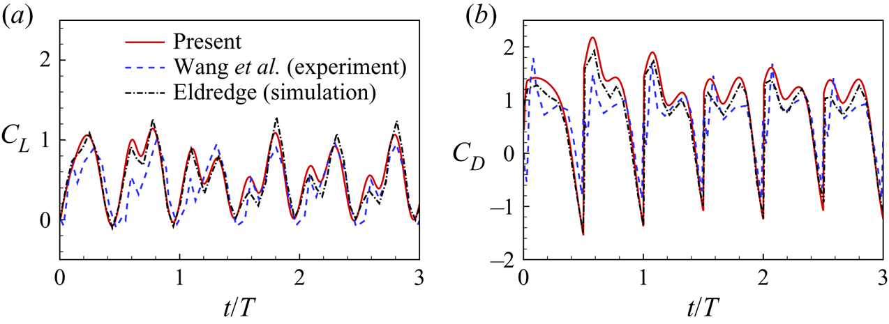
Appendix. Validation of forces experienced by a rigid flapping plate with $Re=75$

We also simulate a rigid flapping case with  $Re = 75$,
 $A/L = 1.4$,
 $\alpha _0 ={\rm \pi} /4$. The problem description is almost identical to that in figure 3(a) except the prescribed translational and rotational motions are applied to the middle of the plate instead of its leading edge. The non-dimensional computational domain size is
 $[-15,25] \times [-15,15]$ and the grid spacing is
 $\Delta x=0.01L$. Both the drag and lift coefficients, i.e.
 $C_D$ and
 $C_L$, as functions of time are shown in figure 19. Here
 $C_L={F_x}/{\frac {1}{2}\rho {U_{ref}}^2 L}$, where
 $F_x$ is the lift force experienced by the plate. It is seen that present results are consistent with those in the experiments of Wang, Birch & Dickinson (Reference Wang, Birch and Dickinson2004) and the simulations of Eldredge (Reference Eldredge2007).
Lift ( $C_L$) and drag (
 $C_D$) coefficients of the rigid flapping plate with
 $Re = 75$,
 $A/L = 1.4$,
 $\alpha _0 ={\rm \pi} /4$. The experimental (Wang et al. Reference Wang, Birch and Dickinson2004) and numerical data (Eldredge Reference Eldredge2007) are also presented.