1 Introduction
The hydrodynamic pilot-wave system discovered by Couder et al. (Reference Couder, Protiere, Fort and Boudaoud2005b ) extends the phenomenological range of classical systems to include behaviour previously thought to be exclusive to microscopic, quantum systems (Bush Reference Bush2015b ; Bush et al. Reference Bush, Couder, Gilet, Milewski and Nachbin2018). The system is characterized by drops, levitated on a vibrating bath, moving in resonance with waves generated by their bouncing at the Faraday frequency. It represents a macroscopic realization of de Broglie’s double-solution pilot-wave theory (de Broglie Reference de Broglie1956), wherein quantum particles move in resonance with a field generated by the particle vibrating at the Compton frequency (Bush Reference Bush2015a ). The dynamics at the Compton scale, specifically the interaction between the particle and wave, was not resolved by de Broglie. Neither is the Compton-scale interaction between a charge and its own electromagnetic field adequately resolved by the Lorentz–Abraham–Dirac equation, the solutions of which break down on the Compton time scale (Hammond Reference Hammond2010). An attractive feature of the walker system is that the fast dynamics responsible for both wave generation and particle propulsion may be resolved both experimentally and theoretically. We thus proceed by resolving experimentally and modelling theoretically the fast, vertical dynamics of bouncing droplets with hopes of providing insights into the walking-droplet system in particular and pilot-wave systems in general.
A regime diagram describing the various bouncing modes of a single drop of radius
 $R$
bouncing on a bath vibrating at a frequency of
 $f=80~\text{Hz}$
with fluid density
 $\unicode[STIX]{x1D70C}=949~\text{kg}~\text{m}^{-3}$
, surface tension
 $\unicode[STIX]{x1D70E}=20.6\times 10^{-3}\text{ N m}^{-1}$
and kinematic viscosity
 $\unicode[STIX]{x1D708}=20\text{ cSt}$
. The vibration number,
 $\unicode[STIX]{x1D6FA}=2\unicode[STIX]{x03C0}f\sqrt{\unicode[STIX]{x1D70C}R^{3}/\unicode[STIX]{x1D70E}}$
, represents the non-dimensional drop size and
 $\unicode[STIX]{x1D6FE}/g$
denotes the dimensionless driving acceleration of the bath, where
 $g$
is the gravitational acceleration. For our experiments, the Faraday threshold was
 $\unicode[STIX]{x1D6FE}_{F}\approx 4.2g$
. Shaded regions denote theoretical bouncing modes obtained using the model of Moláček & Bush (Reference Moláček and Bush2013a
) and markers denote experimentally measured thresholds between them (Wind-Willassen et al.
Reference Wind-Willassen, Moláček, Harris and Bush2013). The drop sizes considered in our study are marked for reference by white lines.

The surface of a fluid bath vibrating vertically with an acceleration
 $\unicode[STIX]{x1D6FE}\text{sin}(\unicode[STIX]{x1D714}t)$
remains flat until the Faraday threshold,
 $\unicode[STIX]{x1D6FE}_{F}$
, above which it destabilizes into a pattern of standing, subharmonic Faraday waves with period
 $T_{F}=4\unicode[STIX]{x03C0}/\unicode[STIX]{x1D714}$
(Benjamin & Ursell Reference Benjamin and Ursell1954; Miles & Henderson Reference Miles and Henderson1990). Millimetric droplets may bounce indefinitely on the surface of the bath for driving accelerations above the bouncing threshold,
 $\unicode[STIX]{x1D6FE}_{B}<\unicode[STIX]{x1D6FE}_{F}$
, exciting spatially extended temporally decaying waves at each impact (Walker Reference Walker1978; Couder et al.
Reference Couder, Fort, Gautier and Boudaoud2005a
; Damiano et al.
Reference Damiano, Brun, Harris, Galeano-Rios and Bush2016). A regime diagram characterizing the dependence of the bouncing motion on a drop’s size and the bath’s driving acceleration is shown in figure 1. The notation
 $(i,j)^{k}$
denotes that a drop’s vertical motion has a period of
 $i$
times that of the bath vibration,
 $T_{F}/2$
, and impacts the bath
 $j$
times during this period;
 $k=\{1,2\}$
distinguishes between relatively small- and large-amplitude bouncers with the same periodicity
 $(i,j)$
(Moláček & Bush Reference Moláček and Bush2013a
). As
 $\unicode[STIX]{x1D6FE}$
is increased progressively beyond
 $\unicode[STIX]{x1D6FE}_{B}$
, the bouncing amplitude of a drop increases and the drop’s vertical motion eventually becomes synchronized with the Faraday waves produced at each bounce, leading to resonant bouncing in the
 $(2,1)$
mode and a substantial increase in the wave amplitude (Protière, Boudaoud & Couder Reference Protière, Boudaoud and Couder2006; Eddi et al.
Reference Eddi, Sultan, Moukhtar, Fort, Rossi and Couder2011b
). As
 $\unicode[STIX]{x1D6FE}$
is further increased beyond the walking threshold,
 $\unicode[STIX]{x1D6FE}_{W}$
, the drop destabilizes into a ‘walker’, a dynamic state in which it moves steadily across the surface of the bath, propelled by its own wavefield (Couder et al.
Reference Couder, Protiere, Fort and Boudaoud2005b
; Protière et al.
Reference Protière, Boudaoud and Couder2006). The local wavefield, the slope of which prescribes the force acting on the walking drop at each impact, depends not only on the drop’s present position but on its past trajectory (Eddi et al.
Reference Eddi, Sultan, Moukhtar, Fort, Rossi and Couder2011b
). The closer the driving acceleration is to the Faraday threshold, the longer the surface waves persist after each impact and the more strongly the drop’s dynamics is affected by its past. This non-Markovian feature of the walking-droplet system is generally referred to as ‘path memory’.
As recently reviewed by Turton, Couchman & Bush (Reference Turton, Couchman and Bush2018), a hierarchy of theoretical models of various degrees of sophistication has been developed to describe walking droplets in a variety of settings (Protière et al.
Reference Protière, Boudaoud and Couder2006; Eddi et al.
Reference Eddi, Sultan, Moukhtar, Fort, Rossi and Couder2011b
; Moláček & Bush Reference Moláček and Bush2013a
,Reference Moláček and Bush
b
; Oza, Rosales & Bush Reference Oza, Rosales and Bush2013; Bush, Oza & Moláček Reference Bush, Oza and Moláček2014; Milewski et al.
Reference Milewski, Galeano-Rios, Nachbin and Bush2015; Dubertrand et al.
Reference Dubertrand, Hubert, Schlagheck, Vandewalle, Bastin and Martin2016; Durey & Milewski Reference Durey and Milewski2017; Faria Reference Faria2017; Galeano-Rios, Milewski & Vanden-Broeck Reference Galeano-Rios, Milewski and Vanden-Broeck2017; Nachbin, Milewski & Bush Reference Nachbin, Milewski and Bush2017). The most sophisticated of such models (Milewski et al.
Reference Milewski, Galeano-Rios, Nachbin and Bush2015; Galeano-Rios et al.
Reference Galeano-Rios, Milewski and Vanden-Broeck2017) involve full numerical simulations of the coupled vertical and horizontal motion of a droplet and so are computationally expensive, with simulations taking
 $10^{2}$
–
 $10^{4}$
times longer than real time. Moláček & Bush (Reference Moláček and Bush2013b
) developed coupled equations describing a walking droplet’s vertical and horizontal motion. By time averaging these equations over a bouncing period, they obtained a ‘stroboscopic’ horizontal trajectory equation, simulation of which requires a computational time comparable to real time. Oza et al. (Reference Oza, Rosales and Bush2013) adapted the time-averaged model of Moláček & Bush (Reference Moláček and Bush2013b
) into an integral model, by treating the walker as a continuous, rather than discrete, source of waves. In the stroboscopic model of Oza et al. (Reference Oza, Rosales and Bush2013), all information about the vertical dynamics is contained in a single fitting parameter
 $-1\leqslant \sin \unicode[STIX]{x1D6F7}\leqslant 1$
, as describes the phase shift between the periodic vertical motion of the bath and the drop at impact.
While the time-averaged, stroboscopic models worked relatively well for capturing the horizontal dynamics of single drops in various scenarios (Moláček & Bush Reference Moláček and Bush2013b
; Oza et al.
Reference Oza, Rosales and Bush2013, Reference Oza, Harris, Rosales and Bush2014a
,Reference Oza, Wind-Willassen, Harris, Rosales and Bush
b
; Labousse et al.
Reference Labousse, Oza, Perrard and Bush2016), significantly different values of
 $\sin \unicode[STIX]{x1D6F7}$
(in the range 0.16–0.5) were used in each of these studies. Further, owing to the assumption of a constant impact phase, the stroboscopic approximation was unable to capture accurately the observed stability of more complicated horizontal trajectories such as the wobbling orbital motion of single drops in a rotating frame (Oza et al.
Reference Oza, Harris, Rosales and Bush2014a
; Labousse et al.
Reference Labousse, Oza, Perrard and Bush2016). Oza et al. (Reference Oza, Siéfert, Harris, Moláček and Bush2017) and Arbelaiz, Oza & Bush (Reference Arbelaiz, Oza and Bush2018) demonstrated that for orbiting (Protière et al.
Reference Protière, Boudaoud and Couder2006; Protière, Bohn & Couder Reference Protière, Bohn and Couder2008) and promenading (Borghesi et al.
Reference Borghesi, Moukhtar, Labousse, Eddi, Fort and Couder2014) droplet pairs, respectively, variations in the vertical dynamics are apparent and significantly influence the pair’s horizontal motion, features that cannot be captured with stroboscopic models. Galeano-Rios et al. (Reference Galeano-Rios, Couchman, Caldairou and Bush2018) have likewise highlighted how subtle variations in a drop’s bouncing phase can change both the speed and the direction of ratcheting droplet pairs (Eddi et al.
Reference Eddi, Terwagne, Fort and Couder2008). Tadrist et al. (Reference Tadrist, Sampara, Schlagheck and Gilet2018a
) have demonstrated that such variations strongly influence the outcome of droplet–droplet scattering events, and may be the source of chaos in a number of hydrodynamic quantum analogues. Perrard & Labousse (Reference Perrard and Labousse2018) suggest that variations in the vertical dynamics may also serve as a mechanism for switching between unstable periodic orbits in orbital pilot-wave dynamics.
In the current study, we develop a reduced model for the coupling between a drop’s vertical and horizontal motion by using the linear spring model developed by Moláček & Bush (Reference Moláček and Bush2013a
) to characterize a drop’s interaction with the bath. This allows us to extend the stroboscopic model of Oza et al. (Reference Oza, Rosales and Bush2013) to account for variations in a drop’s vertical dynamics, without having to resort to a full numerical simulation of the problem. Our model is tested against the results of an experimental investigation of identical droplet pairs, and is found adequate in rationalizing the observed behaviour of the pair as the bath’s driving acceleration,
 $\unicode[STIX]{x1D6FE}$
, is increased progressively.
In § 2, we briefly review the horizontal trajectory equations of Moláček & Bush (Reference Moláček and Bush2013b ) and Oza et al. (Reference Oza, Rosales and Bush2013) as they form the starting point for our theoretical developments. In § 3, we use high-speed imaging to characterize the dependence of a single drop’s impact phase and contact force with the bath on the drop size and the bath’s driving acceleration. Subsequently, we characterize experimentally how neighbouring droplet pairs destabilize into horizontal motion as the bath’s driving acceleration is increased progressively. In § 4, we develop a theoretical model for the impact phase that is consistent with our experimental measurements, and develop a horizontal trajectory equation that accounts for variations in the drop’s vertical dynamics. Using this trajectory equation, we perform a linear stability analysis for identical droplet pairs and show that our variable-phase model provides rationale for the observed instabilities. Finally, in § 5, we discuss applications of our model to systems containing multiple droplets, such as droplet rings and lattices, where variations in the vertical dynamics are also expected to be significant.
2 Prior trajectory equations
Definitions of relevant variables and parameters.

We begin with a brief review of the model of Moláček & Bush (Reference Moláček and Bush2013b
) for the horizontal motion of a bouncing droplet. Definitions of relevant variables and parameters are provided in table 1. The vertical position of the vibrating bath is defined to be
 ${\mathcal{B}}(t)=-(\unicode[STIX]{x1D6FE}/\unicode[STIX]{x1D714}^{2})$
sin
 $(\unicode[STIX]{x1D714}t)$
. The wavefield generated by a single bounce of a drop at
 $(\boldsymbol{x}_{\mathbf{0}},t_{0})$
is described as a standing wave of the form (Moláček & Bush Reference Moláček and Bush2013b
)
 $$\begin{eqnarray}{\mathcal{H}}_{0}(\boldsymbol{x},\boldsymbol{x}_{\mathbf{0}},t,t_{0})=\sqrt{{\displaystyle \frac{2\unicode[STIX]{x1D708}_{e}}{\unicode[STIX]{x03C0}}}}{\displaystyle \frac{mgT_{F}}{\unicode[STIX]{x1D70E}}}{\displaystyle \frac{k_{F}^{3}R^{2}}{3k_{F}^{2}R^{2}+Bo}}{\mathcal{S}}\text{cos}\left({\displaystyle \frac{\unicode[STIX]{x1D714}t}{2}}\right){\displaystyle \frac{J_{0}(k_{F}|\boldsymbol{x}-\boldsymbol{x}_{\mathbf{0}}|)}{\sqrt{t-t_{0}}}}\text{e}^{-(t-t_{0})/(T_{F}M_{e})}.\end{eqnarray}$$
The amplitude of the wave generated at each bounce depends on the drop’s vertical motion through the phase parameter
 $$\begin{eqnarray}{\mathcal{S}}={\displaystyle \frac{\displaystyle \int _{t}^{t+T_{F}}F_{N}(t^{\prime })\text{sin}\left({\displaystyle \frac{\unicode[STIX]{x1D714}t^{\prime }}{2}}\right)\,\text{d}t^{\prime }}{\displaystyle \int _{t}^{t+T_{F}}F_{N}(t^{\prime })\,\text{d}t^{\prime }}}.\end{eqnarray}$$
Here,
 $F_{N}(t)$
is the contact force acting between the drop and the bath and is zero when the drop is in free flight. One contribution of the current study is the first experimental measurements of
 $F_{N}(t)$
for bouncing and walking droplets.
The phase parameter
 ${\mathcal{S}}$
encodes how efficiently the drop generates waves at each impact. In order for the drop to bounce indefinitely, the average force imparted by the bath on the drop must balance the drop’s weight. For a drop in a (2,1) bouncing mode, this balance may be expressed as
 $\int _{t}^{t+T_{F}}F_{N}(t^{\prime })\,\text{d}t^{\prime }=mgT_{F}$
(Moláček & Bush Reference Moláček and Bush2013b
). Evidently, it is the phase of the contact force relative to the bath’s oscillation that governs the amplitude of the wave generated at each bounce. Moláček & Bush (Reference Moláček and Bush2013b
) assumed that the waves generated at each impact are dominated by modes with a wavenumber close to the Faraday wavenumber,
 $k_{F}$
. Consequently, the phase parameter
 ${\mathcal{S}}$
, the first coefficient in a Fourier series expansion of
 $F_{N}(t)$
, captures the dominant response of the bath to the impacting droplet. A recent review of the wave model of Moláček & Bush (Reference Moláček and Bush2013b
) and a further discussion of
 ${\mathcal{S}}$
is provided in Turton et al. (Reference Turton, Couchman and Bush2018).
We note that the wavefield described by (2.1) has been found to have insufficient spatial decay for
 $|\boldsymbol{x}-\boldsymbol{x}_{\mathbf{0}}|\gtrsim \unicode[STIX]{x1D706}_{F}$
, prompting a correction to the wave model in the form of a spatio-temporal damping factor (Damiano et al.
Reference Damiano, Brun, Harris, Galeano-Rios and Bush2016; Oza et al.
Reference Oza, Siéfert, Harris, Moláček and Bush2017; Turton et al.
Reference Turton, Couchman and Bush2018). When modelling the dynamics of single drops, we neglect this correction as the drop is primarily influenced by waves produced within a distance
 $\unicode[STIX]{x1D706}_{F}$
of the drop’s current position. For instance, consider a drop walking at a speed
 $u=10~\text{mm}~\text{s}^{-1}$
at
 $\unicode[STIX]{x1D6FE}/\unicode[STIX]{x1D6FE}_{F}=0.85$
. Once the drop has moved a distance
 $\unicode[STIX]{x1D706}_{F}$
from a previous impact, the wave produced at that impact will have decayed to
 $\exp [-\unicode[STIX]{x1D706}_{F}/(uT_{F}M_{e})]\approx 2\,\%$
of its original amplitude. Hence, the far-field behaviour of the pilot wave has a negligible effect on the motion of a single walker executing rectilinear motion. However, it is significant when modelling droplet–droplet interactions, as is evident in our study of droplet pairs (see § 4.2).
Moláček & Bush (Reference Moláček and Bush2013b ) derived the following trajectory equation for the horizontal motion of a droplet:
 $$\begin{eqnarray}m\ddot{\boldsymbol{x}}_{p}+\left(C\sqrt{{\displaystyle \frac{\unicode[STIX]{x1D70C}R}{\unicode[STIX]{x1D70E}}}}F_{N}(t)+6\unicode[STIX]{x03C0}R\unicode[STIX]{x1D707}_{a}\right)\dot{\boldsymbol{x}}_{p}=-F_{N}(t)\unicode[STIX]{x1D735}{\mathcal{H}}(\boldsymbol{x}_{p},t),\end{eqnarray}$$
where the net wavefield,
 $$\begin{eqnarray}{\mathcal{H}}(\boldsymbol{x},t)=\mathop{\sum }_{n}{\mathcal{H}}_{n}(\boldsymbol{x},\boldsymbol{x}_{\boldsymbol{n}},t,t_{n}),\end{eqnarray}$$
with
 ${\mathcal{H}}_{n}$
described by (2.1), is assumed to be the linear superposition of the waves generated by the drop at each previous bounce. When in contact with the bath, the drop receives a horizontal impulse proportional to the gradient of the wavefield at the point of impact and weighted by
 $F_{N}(t)$
. The drop’s horizontal motion is resisted by air drag and an additional drag force imparted by the bath during impact that is proportional to
 $F_{N}(t)$
. In order to solve equation (2.3), a model for a drop’s vertical motion is required to obtain
 $F_{N}(t)$
. In the inelastic ball model of Gilet, Vandewalle & Dorbolo (Reference Gilet, Vandewalle and Dorbolo2009),
 $F_{N}(t)$
is not specified; however, the form of
 $F_{N}(t)$
could be deduced from the linear spring model of Terwagne et al. (Reference Terwagne, Ludewig, Vandewalle and Dorbolo2013). Moláček & Bush (Reference Moláček and Bush2013a
) have developed both linear and logarithmic spring models for the drop’s vertical motion from which
 $F_{N}(t)$
can be inferred directly. It is computationally expensive to simulate simultaneously the horizontal and vertical dynamics of a drop (Milewski et al.
Reference Milewski, Galeano-Rios, Nachbin and Bush2015; Galeano-Rios et al.
Reference Galeano-Rios, Milewski and Vanden-Broeck2017); thus, the majority of subsequent models (Oza et al.
Reference Oza, Rosales and Bush2013; Bush et al.
Reference Bush, Oza and Moláček2014; Dubertrand et al.
Reference Dubertrand, Hubert, Schlagheck, Vandewalle, Bastin and Martin2016; Durey & Milewski Reference Durey and Milewski2017; Faria Reference Faria2017; Nachbin et al.
Reference Nachbin, Milewski and Bush2017) have not accounted for variability in the vertical dynamics.
To make theoretical headway, Moláček & Bush (Reference Moláček and Bush2013b
) focused on drops in the resonant
 $(2,1)$
bouncing mode, where the time scale of a drop’s vertical motion,
 $T_{F}=0.025$
s, is much smaller than that of the drop’s horizontal motion,
 $\unicode[STIX]{x1D706}_{F}/|\dot{\boldsymbol{x}}_{p}|\approx 0.5$
s. Time-averaging equation (2.3) over a
 $(2,1)$
bouncing period,
 $T_{F}$
, yields a ‘stroboscopic’ horizontal trajectory equation (Moláček & Bush Reference Moláček and Bush2013b
),
 $$\begin{eqnarray}m\ddot{\boldsymbol{x}}_{p}+D\dot{\boldsymbol{x}}_{p}=-mg{\mathcal{C}}\unicode[STIX]{x1D735}h(\boldsymbol{x}_{p},t),\end{eqnarray}$$
where
 $h={\mathcal{H}}/\text{cos}(\unicode[STIX]{x1D714}t/2)$
represents the wavefield strobed at the drop’s bouncing period. As the wavefield,
 ${\mathcal{H}}$
, on the bath surface (2.1) oscillates in time as
 $\cos (\unicode[STIX]{x1D714}t/2)$
, the gradient of the wavefield experienced by the droplet will depend on when in the wavefield’s cycle the drop impacts. Since the impact is not instantaneous, the average horizontal impulse exerted by the wave on the drop is modelled as
 $-mg{\mathcal{C}}\unicode[STIX]{x1D735}h(\boldsymbol{x}_{p},t)$
, where the phase parameter
 $$\begin{eqnarray}{\mathcal{C}}={\displaystyle \frac{\displaystyle \int _{t}^{t+T_{F}}F_{N}(t^{\prime })\text{cos}\left({\displaystyle \frac{\unicode[STIX]{x1D714}t^{\prime }}{2}}\right)\,\text{d}t^{\prime }}{\displaystyle \int _{t}^{t+T_{F}}F_{N}(t^{\prime })\,\text{d}t^{\prime }}}\end{eqnarray}$$
represents the average phase of impact with respect to the oscillating wavefield, weighted by the normal force
 $F_{N}(t)$
. As a first-order approximation, Moláček & Bush (Reference Moláček and Bush2013b
) assumed that the phase parameters
 ${\mathcal{S}}$
and
 ${\mathcal{C}}$
were constants and replaced the product
 ${\mathcal{S}}{\mathcal{C}}$
in (2.5) by the fitting parameter
 $\sin (\unicode[STIX]{x1D6F7})/2$
, which then contains all the information about the bouncing phase.
Finally, for analytic simplicity, Oza et al. (Reference Oza, Rosales and Bush2013) approximated the drop to be a continuous rather than discrete source of waves, resulting in the trajectory equation
 $$\begin{eqnarray}m\ddot{\boldsymbol{x}}_{p}+D\dot{\boldsymbol{x}}_{p}=-{\displaystyle \frac{mg\sin \unicode[STIX]{x1D6F7}}{2}}\unicode[STIX]{x1D735}h(\boldsymbol{x}_{p},t),\end{eqnarray}$$
where
 $$\begin{eqnarray}h(\boldsymbol{x},t)=\sqrt{{\displaystyle \frac{2\unicode[STIX]{x1D708}_{e}}{\unicode[STIX]{x03C0}T_{F}}}}{\displaystyle \frac{mgk_{F}^{3}R^{2}}{\unicode[STIX]{x1D70E}(3k_{F}^{2}R^{2}+Bo)}}\displaystyle \int _{-\infty }^{t}J_{0}(k_{F}|\boldsymbol{x}-\boldsymbol{x}_{p}(s)|)\text{e}^{-(t-s)/(T_{F}M_{e})}\,\text{d}s.\end{eqnarray}$$
We note that when Oza et al. (Reference Oza, Rosales and Bush2013) approximated the sum in the wave model of Moláček & Bush (Reference Moláček and Bush2013b
) (2.4) by an integral (2.8), the decay factor
 $1/\sqrt{t}$
was approximated by
 $1/\sqrt{T_{F}}$
for simplicity, as it was assumed to be sub-dominant to the exponential temporal decay. However, as shown in appendix A, this approximation causes the amplitude of the wave built up after many bounces to be approximately twice that predicted by Moláček & Bush (Reference Moláček and Bush2013b
). Thus, Moláček & Bush (Reference Moláček and Bush2013b
) and Oza et al. (Reference Oza, Rosales and Bush2013) were obliged to use different values of
 $\sin \unicode[STIX]{x1D6F7}$
, 0.5 and 0.3 respectively, in order to fit the same experimental data detailing the dependence of a drop’s walking speed on
 $\unicode[STIX]{x1D6FE}$
. In this study, we wish to adopt the continuous model of Oza et al. (Reference Oza, Rosales and Bush2013), as it is more analytically tractable than the discrete model of Moláček & Bush (Reference Moláček and Bush2013b
). However, as we wish to eliminate
 $\sin \unicode[STIX]{x1D6F7}$
as a fitting parameter, we require that the wave amplitude of our model be consistent with that of Moláček & Bush (Reference Moláček and Bush2013b
), which has been found to be in good agreement with experimentally measured wavefields (Damiano et al.
Reference Damiano, Brun, Harris, Galeano-Rios and Bush2016). Thus, we proceed by dividing the wave amplitude of Oza et al. (Reference Oza, Rosales and Bush2013) in (2.8) by a factor of 2, so that it approximately matches that of Moláček & Bush (Reference Moláček and Bush2013b
).
Using the dimensionless variables
 $\bar{\boldsymbol{x}}=k_{F}\boldsymbol{x}$
,
 $\bar{h}=h/R$
and
 $\bar{t}=t/(T_{F}M_{e})$
, the trajectory equation (2.7) of Oza et al. (Reference Oza, Rosales and Bush2013) becomes
 $$\begin{eqnarray}\unicode[STIX]{x1D705}\ddot{\bar{\boldsymbol{x}}}_{p}+\dot{\bar{\boldsymbol{x}}}_{p}=-\unicode[STIX]{x1D6FD}{\mathcal{C}}\unicode[STIX]{x1D735}\bar{h}(\bar{\boldsymbol{x}}_{p},\bar{t}),\end{eqnarray}$$
where
 $$\begin{eqnarray}\bar{h}(\bar{\boldsymbol{x}},\bar{t})={\displaystyle \frac{AM_{e}}{R}}\displaystyle \displaystyle \int _{-\infty }^{\bar{t}}{\mathcal{S}}J_{0}(|\bar{\boldsymbol{x}}-\bar{\boldsymbol{x}}_{p}(\bar{s})|)\text{e}^{-(\bar{t}-\bar{s})}\,\text{d}\bar{s}.\end{eqnarray}$$
Note that the wave-amplitude coefficient,
 $A$
(see table 1), has been corrected to be consistent with that of Moláček & Bush (Reference Moláček and Bush2013b
). We proceed by determining the dependence of the phase parameters
 ${\mathcal{S}}$
and
 ${\mathcal{C}}$
on the driving acceleration of the bath,
 $\unicode[STIX]{x1D6FE}$
, the local wave amplitude at the location of a drop’s impact,
 $h_{p}=h(\boldsymbol{x}_{p},t)$
and the drop radius,
 $R$
, both experimentally and theoretically. This will allow the horizontal trajectory equation (2.9) to capture the subtle coupling between the drop’s vertical and horizontal motion.
(a) A schematic diagram of the experimental set-up. A detailed description of the shaker used to vibrate the bath is given in Harris & Bush (Reference Harris and Bush2015). A high-speed camera and an overhead camera are used to record the vertical and horizontal motion of a drop, respectively. A Plexiglas enclosure surrounds the bath to eliminate the influence of air currents on the motion of the droplet. (b) A snapshot of a bouncing droplet captured with the high-speed camera. The dark region at the top of the image is the far edge of the bath and appears out of focus due to the small depth of field of the magnifying lens. (c) Thresholding the image in (b) allows us to track the vertical positions of both the drop’s top,
 $z_{T}$
, and the bath’s edge,
 ${\mathcal{B}}$
, and so infer the phase difference between the bouncing motion and the bath vibration.

3 Experiments
Experiments were performed using the set-up described in Harris & Bush (Reference Harris and Bush2015) (see figure 2
a). A bath of silicon oil (density
 $\unicode[STIX]{x1D70C}=949~\text{kg}~\text{m}^{-3}$
, surface tension
 $\unicode[STIX]{x1D70E}=20.6\times 10^{-3}~\text{N}~\text{m}^{-1}$
, kinematic viscosity
 $\unicode[STIX]{x1D708}=20~\text{cSt}$
) was sinusoidally shaken in the vertical direction with a frequency of
 $f=80$
Hz. Droplets of a desired size, composed of the same silicon oil, were created using a piezoelectric droplet generator (Harris, Liu & Bush Reference Harris, Liu and Bush2015). In § 3.1, we characterize the dependence of the phase parameters
 ${\mathcal{S}}$
and
 ${\mathcal{C}}$
on the drop radius,
 $R$
, and the driving acceleration of the bath,
 $\unicode[STIX]{x1D6FE}$
, for single bouncers and walkers. In § 3.2, we consider bound pairs of identical drops and characterize both their vertical motion and destabilization into horizontal motion as
 $\unicode[STIX]{x1D6FE}$
is increased progressively.
3.1 Single drops
We measure the vertical dynamics of drops of three different radii,
 $R=0.32$
mm,
 $R=0.36$
mm and
 $R=0.40$
mm, across the range of driving accelerations from
 $\unicode[STIX]{x1D6FE}=2.5g$
to
 $\unicode[STIX]{x1D6FE}=4.2g$
, in increments of
 $0.1g$
. This parameter space was chosen to focus on drops in the
 $(2,1)$
bouncing and walking regimes (see figure 1) in which the resonance between drop and wave assumed in the derivations of the trajectory equations of Moláček & Bush (Reference Moláček and Bush2013b
) and Oza et al. (Reference Oza, Rosales and Bush2013) is achieved.
In order to compute
 ${\mathcal{S}}$
and
 ${\mathcal{C}}$
for a given
 $R$
and
 $\unicode[STIX]{x1D6FE}$
, we used the following procedure. A high-speed camera (Phantom v5.2, macro lens,
 $2\times$
teleconverter, tube extension) was used to record simultaneously the motion of the drop and the bath at a frame rate of 3000 fps, corresponding to 75 frames per Faraday period,
 $T_{F}$
. A snapshot from one of these videos is shown in figure 2(b). The dark stripe at the top of the frame corresponds to the far edge of the bath and is out of focus due to the small depth of field of the magnifying lens. As shown in figure 2(c), this same frame can be thresholded to yield an outline of the drop’s edge, the top of which we denote by
 $z_{T}$
, and a horizontal line near the top of the frame, representing the vertical position of the bath’s edge,
 ${\mathcal{B}}$
. By thresholding each frame in the video, we obtain time series
 ${\mathcal{B}}(t)$
and
 $z_{T}(t)$
, examples of which are shown in figures 3(a,b). If a droplet was walking, it was recorded as it moved through the high-speed camera’s field of view while the overhead camera simultaneously recorded its horizontal motion.
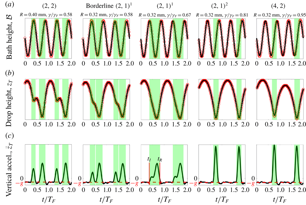
Examples of the time evolution of (a) the bath’s vertical position, (b) the drop’s vertical position and (c) the drop’s vertical acceleration for the five bouncing modes observed in our experiments. The Faraday period is
 $T_{F}=1/40$
s. The red data points in (a) and (b) are obtained by tracking the vertical position of the bath’s edge and the top of the drop respectively. For the sake of comparison, pure sinusoids with the bath’s oscillation frequency of 80 Hz are plotted with solid lines in (a). The solid lines in (b) are the result of applying the smoothing Savitzky–Golay filter to the experimental data, which are then differentiated twice to obtain the drop’s vertical acceleration reported in (c). The red dashed lines in (c) indicate the free-fall acceleration,
 $-g$
. Each green shaded region indicates a calculated period of contact between the drop and the bath, starting at the time of drop impact,
 $t_{I}$
, and ending at the time of drop release,
 $t_{R}$
. The vertical scales in (a) and (b) are arbitrary.

The contact force,
 $F_{N}(t)$
, can be computed directly from
 $z_{T}(t)$
. A Savitzky–Golay filter is used to compute the drop’s vertical acceleration,
 $\ddot{z}_{T}$
(figure 3
c). The acceleration of the top of the drop provides a good approximation to the acceleration of the drop’s centre of mass provided the drop deformation during impact is small. In our experiments, the maximum deformation observed is
 ${\approx}5\,\%$
of the undeformed drop diameter. The regions of constant acceleration in the time series of
 $\ddot{z}_{T}$
occur when the drop is in free flight, with acceleration
 $-g$
, while the regions of increased acceleration, shaded in green in figure 3(c), occur when the drop is in contact with the bath;
 $F_{N}(t)$
is then obtained by subtracting the free-fall acceleration,
 $-g$
, from
 $\ddot{z}_{T}$
and is necessarily zero when the drop is not in contact with the bath. We note that when a drop is walking in a straight line at a constant speed, the vertical position recorded by the high-speed camera will be of the form
 $z_{T}(t)+at+b$
, where
 $z_{T}(t)$
would be the vertical position recorded if the drop was bouncing in place and the linear function reflects the drop’s translation across the camera’s field of view. Since the linear function
 $at+b$
makes no contribution to the second derivative, the drop’s horizontal motion does not affect the computed vertical acceleration. When a drop is near the
 $(2,2)$
to
 $(2,1)^{1}$
transition, it is difficult to characterize the bouncing mode (Galeano-Rios et al.
Reference Galeano-Rios, Milewski and Vanden-Broeck2017). We classify a drop as being in a ‘borderline’
 $(2,1)^{1}$
mode when two distinct impacts per Faraday period are discernible by analysing
 $F_{N}(t)$
in figure 3(c), but the droplet does not rebound upwards between these impacts, as determined by analysing
 $z_{T}(t)$
in figure 3(b).
The dependence of (a) the phase parameter
 ${\mathcal{S}}$
, (b) the phase parameter
 ${\mathcal{C}}$
and (c) the walking speed,
 $u$
, on the non-dimensional driving acceleration of the bath,
 $\unicode[STIX]{x1D6FE}/\unicode[STIX]{x1D6FE}_{F}$
, for single bouncing drops of size
 $R=0.32$
mm (red),
 $R=0.36$
mm (green) and
 $R=0.40$
mm (blue). The unfilled and filled markers indicate experimental data and denote whether the droplet is bouncing or walking, respectively. The shape of the marker denotes the experimentally observed bouncing mode:
 $(2,2)$
mode (*), borderline
 $(2,1)^{1}$
mode (
 $\star$
),
 $(2,1)^{1}$
mode (▫),
 $(2,1)^{2}$
mode (▵),
 $(4,2)$
mode (○). Characteristic error bars are shown. In (a) and (b) the dotted and solid curves are the corresponding theoretical predictions (see § 4.1) and denote whether the droplet is predicted to bounce or walk, respectively. For values of
 $\unicode[STIX]{x1D6FE}$
where (*), (
 $\star$
) or (▫) bouncing modes were experimentally observed, the
 $(2,1)^{1}$
phase functions of the form given in table 2 are used for the theoretical predictions. For (▵) and (○) modes, the
 $(2,1)^{2}$
phase functions are used. The discontinuities in the theoretical curves occur at the
 $(2,1)^{1}$
to
 $(2,1)^{2}$
transitions. In (c), the solid and dashed lines represent, respectively, the walking speeds predicted by our variable-impact-phase trajectory equation (see § 4.1) and the constant-impact-phase trajectory equation of Oza et al. (Reference Oza, Rosales and Bush2013).

Our direct measurements of the vertical motion of both bouncing and walking droplets will be valuable in benchmarking and guiding the development of theoretical models. Our measurements of the contact times and contact forces across a range of bouncing modes (figure 3) are very similar to those predicted theoretically by the droplet impact models of Milewski et al. (Reference Milewski, Galeano-Rios, Nachbin and Bush2015) and Galeano-Rios et al. (Reference Galeano-Rios, Milewski and Vanden-Broeck2017). For example, comparing figure 3c to figures 8 and 11 in Galeano-Rios et al. (Reference Galeano-Rios, Milewski and Vanden-Broeck2017) indicates that the model of Galeano-Rios et al. (Reference Galeano-Rios, Milewski and Vanden-Broeck2017) accurately captures the
 $(2,2)$
to
 $(2,1)^{1}$
to
 $(2,1)^{2}$
progression in bouncing modes as
 $\unicode[STIX]{x1D6FE}$
is increased. For a drop in the
 $(2,2)$
mode, as
 $\unicode[STIX]{x1D6FE}$
is increased progressively, the contact force during the first impact decreases relative to that during the second impact, and the time of flight between these two impacts also decreases. At the critical
 $\unicode[STIX]{x1D6FE}$
value at which these two initially separate impacts merge, the drop becomes a
 $(2,1)^{1}$
bouncer. As
 $\unicode[STIX]{x1D6FE}$
is further increased, the time of the drop’s release from the bath,
 $t_{R}$
, remains approximately constant, while the time of impact,
 $t_{I}$
, moves progressively closer to
 $t_{R}$
until the drop eventually enters a
 $(2,1)^{2}$
mode.
Once
 $F_{N}(t)$
is computed, the trapezoidal rule is used to numerically calculate
 ${\mathcal{S}}$
(2.2) and
 ${\mathcal{C}}$
(2.6). When performing the integrals, the time
 $t=0$
is defined such that
 ${\mathcal{B}}(t)=-(\unicode[STIX]{x1D6FE}/\unicode[STIX]{x1D714}^{2})\sin (\unicode[STIX]{x1D714}t)$
. For each
 $R$
and
 $\unicode[STIX]{x1D6FE}$
, approximately 20 bounces were recorded and the phase parameters were computed for each bounce and then averaged. The standard deviation of the phase parameters before averaging is of the order of 1 %. To compute
 $S$
and
 $C$
for drops in a
 $(4,2)$
mode, the integrals in (2.2) and (2.6) were evaluated from
 $t$
to
 $t+2T_{F}$
. We emphasize that
 ${\mathcal{S}}$
and
 ${\mathcal{C}}$
represent average impact phases weighted by the contact force
 $F_{N}(t)$
. We have observed that within the
 $(2,1)^{2}$
mode, the times of drop impact,
 $t_{I}$
, and release,
 $t_{R}$
, from the bath may remain approximately constant as
 $\unicode[STIX]{x1D6FE}$
is increased. Thus, one might infer that the drop’s impact phase is independent of
 $\unicode[STIX]{x1D6FE}$
. However, even when
 $t_{I}$
and
 $t_{R}$
remain constant, the profile
 $F_{N}(t)$
for
 $t_{I}\leqslant t\leqslant t_{R}$
shifts as
 $\unicode[STIX]{x1D6FE}$
increases, resulting in changes to both
 ${\mathcal{S}}$
and
 ${\mathcal{C}}$
. Hence, knowledge of the time dependence of the contact force is critical in order to model effectively the coupling between the drop’s horizontal and vertical motion.
The dependences of
 ${\mathcal{S}}$
,
 ${\mathcal{C}}$
and the walking speed,
 $u$
, on
 $R$
and
 $\unicode[STIX]{x1D6FE}$
are shown in figure 4. Both
 ${\mathcal{S}}$
and
 ${\mathcal{C}}$
are seen to have two distinct trends separated by the
 $(2,1)^{1}$
to
 $(2,1)^{2}$
transition. Before this transition, both
 ${\mathcal{S}}$
and
 ${\mathcal{C}}$
increase approximately linearly with
 $\unicode[STIX]{x1D6FE}$
, while after the transition
 ${\mathcal{S}}$
saturates to a constant value of approximately 1 while
 ${\mathcal{C}}$
decreases monotonically.
3.2 Pairs of identical drops
The dependence of the inter-drop separation distance,
 $d$
, on the dimensionless driving acceleration,
 $\unicode[STIX]{x1D6FE}/\unicode[STIX]{x1D6FE}_{F}$
, for stable, bound droplet pairs of radius
 $R=0.32$
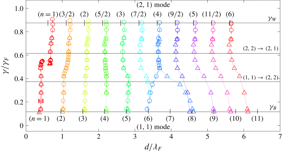
mm. Circles indicate data obtained by increasing the driving acceleration and triangles indicate data obtained by lowering it again. The top-most data points indicate the instability thresholds,
 $\unicode[STIX]{x1D6FE}_{\ast }$
, at which the stationary pairs go unstable to horizontal motion, in a manner detailed in figure 7. A characteristic error bar is shown for an
 $n=1$
data point. The bouncing threshold
 $\unicode[STIX]{x1D6FE}_{B}$
,
 $(1,1)\rightarrow (2,2)$
transition,
 $(2,2)\rightarrow (2,1)$
transition, and walking threshold,
 $\unicode[STIX]{x1D6FE}_{W}$
, for a single drop of radius
 $R=0.32$
mm are shown for reference. The vertical ticks along the horizontal lines denoting
 $\unicode[STIX]{x1D6FE}_{B}$
and
 $\unicode[STIX]{x1D6FE}_{W}$
indicate the stable separation distances,
 $d_{n}$
, predicted by our theoretical model (see § 4.3).

We proceed by highlighting the critical role of bouncing phase variations on the bouncing to walking transition of identical droplet pairs. As shown by Eddi et al. (Reference Eddi, Decelle, Fort and Couder2009), droplet pairs can exist in a discrete set of bound states corresponding to each drop bouncing in a minimum of its neighbour’s wavefield. The quantized set of possible inter-drop separation distances,
 $d_{n}$
, is characterized by the binding number
 $n=\{1,3/2,2,5/2,\ldots ,\}$
, where integers and half-integers denote pairs bouncing in- and out-of-phase, respectively (Eddi et al.
Reference Eddi, Decelle, Fort and Couder2009). We consider the behaviour of bouncing pairs of two different radii,
 $R=0.32$
mm and
 $R=0.40$
mm, with various binding numbers
 $n$
, as
 $\unicode[STIX]{x1D6FE}$
is increased progressively. These sizes were chosen to ensure that, close to their instability thresholds, the pairs had different vertical dynamics, specifically, the larger and smaller pairs are in
 $(2,1)^{1}$
and
 $(2,1)^{2}$
bouncing modes, respectively.
For each pair size,
 $\unicode[STIX]{x1D6FE}$
is set slightly above the bouncing threshold for a single drop,
 $\unicode[STIX]{x1D6FE}_{B}$
, and two identical drops are created that bounce in a
 $(1,1)$
mode. As
 $(1,1)$
pairs bounce with the same period as the vibrating bath they can only bounce in phase. It was possible to initialize
 $(1,1)$
pairs in six binding numbers
 $n\in [1,6]$
(see figure 5). Our findings extend the work of Eddi et al. (Reference Eddi, Decelle, Fort and Couder2009) who reported three possible
 $n\in [1,3]$
, for
 $(1,1)$
pairs. Pairs starting with a different, intermediate
 $d$
, spontaneously adjust their spacing to reach the closest stable
 $d_{n}$
. For each
 $(1,1)$
pair in
 $n\in [1,6]$
, we increased
 $\unicode[STIX]{x1D6FE}$
incrementally, causing the inter-drop distances to evolve as reported in figure 5, as the pairs transitioned from
 $(1,1)$
to
 $(2,1)$
bouncing modes. We note that as
 $\unicode[STIX]{x1D6FE}$
is increased, the bouncing phase can flip spontaneously. For example, in-phase
 $n=2$
and
 $n=4$
 $(1,1)$
pairs end up as out-of-phase
 $n=3/2$
and
 $n=5/2$
 $(2,1)$
pairs, respectively. The
 $(2,1)$
pairs ultimately go unstable to horizontal motion at
 $\unicode[STIX]{x1D6FE}=\unicode[STIX]{x1D6FE}_{\ast }$
, indicated by the top-most data points in figure 5. For pairs of size
 $R=0.32$
mm, the instability threshold,
 $\unicode[STIX]{x1D6FE}_{\ast }$
, occurs above the walking threshold of a single drop,
 $\unicode[STIX]{x1D6FE}_{W}$
, as shown in detail in figure 7.
Due to the increased amplitude and spatial extent of a drop’s wavefield close to
 $\unicode[STIX]{x1D6FE}_{\ast }$
,
 $(2,1)$
pairs could be initialized with larger binding numbers
 $n$
that were not accessible in the vicinity of
 $\unicode[STIX]{x1D6FE}_{B}$
. As shown in figure 5, eleven possible
 $n$
were found for
 $(2,1)$
pairs, as compared to the six reported by Eddi et al. (Reference Eddi, Decelle, Fort and Couder2009). For each new
 $n$
, a
 $(2,1)$
pair was initialized at a driving acceleration slightly below the anticipated instability threshold, and
 $\unicode[STIX]{x1D6FE}$
was then increased until
 $\unicode[STIX]{x1D6FE}_{\ast }$
was found. For each of the eleven
 $(2,1)$
binding numbers
 $n$
, we also progressively decreased
 $\unicode[STIX]{x1D6FE}$
until the pairs coalesced with the bath. This progression revealed hysteresis in the dependence of
 $d$
on
 $\unicode[STIX]{x1D6FE}$
as well as the existence of additional
 $(1,1)$
binding numbers up to
 $n=11$
. These additional states were impossible to achieve by initializing the pairs in the vicinity of
 $\unicode[STIX]{x1D6FE}_{B}$
due to the weakness of the droplet–droplet interaction at such large
 $n$
and low
 $\unicode[STIX]{x1D6FE}$
. For drops of radius
 $R=0.40$
mm, the dependence of
 $d$
on
 $\unicode[STIX]{x1D6FE}$
and
 $n$
is very similar to that presented in figure 5, except that the instability thresholds,
 $\unicode[STIX]{x1D6FE}_{\ast }$
, occur below the walking threshold of an individual drop,
 $\unicode[STIX]{x1D6FE}_{W}$
, as shown in figure 7.
In addition to measuring the inter-drop distance
 $d$
, we used the technique presented in § 3.1 to measure the phase parameters
 ${\mathcal{S}}$
and
 ${\mathcal{C}}$
for drops in period-doubled
 $(2,1)$
pairs with binding numbers
 $n=1$
and
 $n=2$
. The results are presented in figure 6. For drops in the
 $(2,1)^{1}$
mode, both
 ${\mathcal{S}}$
and
 ${\mathcal{C}}$
increase with decreasing
 $n$
. For drops in the
 $(2,1)^{2}$
mode,
 ${\mathcal{S}}$
has saturated to 1 and does not depend strongly on
 $n$
, while
 ${\mathcal{C}}$
now decreases with decreasing
 $n$
. Notably, the bouncing mode transitions are different when the drops are in pairs. Specifically, the
 $(2,2)\rightarrow (2,1)^{1}$
,
 $(2,1)^{1}\rightarrow (2,1)^{2}$
, and
 $(2,1)^{2}\rightarrow (4,2)$
transitions occur at lower values of
 $\unicode[STIX]{x1D6FE}$
than for single drops, and these values decrease monotonically with decreasing
 $n$
.
The dependence of the phase parameters
 ${\mathcal{S}}$
and
 ${\mathcal{C}}$
on the non-dimensional driving acceleration,
 $\unicode[STIX]{x1D6FE}/\unicode[STIX]{x1D6FE}_{F}$
, for bouncing pairs of size
 $R=0.32$
mm and
 $R=0.40$
mm with binding numbers
 $n=1$
(red) and
 $n=2$
(green). The corresponding data for a single bouncer, from figure 4(a,b), are shown for reference, in black. The shape of each data point indicates the bouncing mode:
 $(2,2)$
mode (*), borderline
 $(2,1)^{1}$
mode (
 $\star$
),
 $(2,1)^{1}$
mode (▫),
 $(2,1)^{2}$
mode (▵),
 $(4,2)$
mode (○). Characteristic error bars are shown. Data were collected up until the instability threshold,
 $\unicode[STIX]{x1D6FE}_{\ast }$
, at which the pair went unstable to horizontal motion. Theoretical predictions of our variable-phase model (see § 4.3) are shown for reference by solid curves.

The instability thresholds,
 $\unicode[STIX]{x1D6FE}_{\ast }$
, and type of instability for identical droplet pairs of radius
 $R=0.40\text{ mm}$
(blue) and
 $R=0.32\text{ mm}$
(red), as are in
 $(2,1)^{1}$
and
 $(2,1)^{2}$
bouncing modes, respectively. Circles denote experimental data and the squares connected by dashed lines are the theoretical predictions of the variable-phase model presented in § 4.3. Characteristic error bars are shown. Note that the experimental data for
 $R=0.32\text{ mm}$
correspond to the top most data points in figure 5. The instability thresholds are normalized by the walking threshold of a single drop,
 $\unicode[STIX]{x1D6FE}_{W}$
, as was measured to be
 $\unicode[STIX]{x1D6FE}_{W}\approx 0.77\unicode[STIX]{x1D6FE}_{F}$
and
 $\unicode[STIX]{x1D6FE}_{W}\approx 0.88\unicode[STIX]{x1D6FE}_{F}$
for drops of size
 $R=0.40$
mm and
 $R=0.32$
mm, respectively. The type of instability predicted by the theoretical model is discussed in § 4.3.

In figure 7, we show the dependence of a pair’s instability threshold,
 $\unicode[STIX]{x1D6FE}_{\ast }$
, on the binding number,
 $n$
, for the two drop sizes considered. The larger pair, of radius
 $R=0.40$
mm, bounces in a
 $(2,1)^{1}$
mode in the vicinity of
 $\unicode[STIX]{x1D6FE}_{\ast }$
and destabilizes below the walking threshold of an individual drop,
 $\unicode[STIX]{x1D6FE}_{W}$
. For all
 $n$
, the pair destabilizes into oscillations along the line connecting the drops, which we refer to henceforth as co-linear oscillations. An example of the onset of co-linear oscillations is shown in figure 8(a). Conversely, the smaller pair, of radius
 $R=0.32$
mm, bounces in a
 $(2,1)^{2}$
mode in the vicinity of
 $\unicode[STIX]{x1D6FE}_{\ast }$
and goes unstable above
 $\unicode[STIX]{x1D6FE}_{W}$
. For the smaller pair, the type of instability now depends on
 $n$
. An
 $n=1$
pair goes unstable to orbital motion (figure 8
b) while pairs in higher
 $n>1$
, go unstable to promenading states, in which the drops walk side-by-side (Borghesi et al.
Reference Borghesi, Moukhtar, Labousse, Eddi, Fort and Couder2014; Arbelaiz et al.
Reference Arbelaiz, Oza and Bush2018). Promenading pairs with
 $n=\{3/2,2,5/2\}$
move in straight lines (figure 8
c), while pairs with
 $n\geqslant 3$
exhibit lateral oscillations (figure 8
d). We note that for pairs of size
 $R=0.32$
mm, the type of instability is sensitive to small size variations between the two drops. Specifically, if the size variation is
 ${\gtrsim}5\,\%$
, the difference in walking thresholds between the two drops causes one drop to orbit the other, which initially remains stationary. Orbital motion then occurs at most separation distances, not just for the
 $n=1$
pair. As seen in figure 7, for both pair sizes,
 $\unicode[STIX]{x1D6FE}_{\ast }$
tends to
 $\unicode[STIX]{x1D6FE}_{W}$
as
 $n$
increases, due to the interaction between the drops decreasing with increasing
 $n$
.
Examples of the onset of instability of bound droplet pairs: (a) co-linear oscillations (
 $R=0.40$
mm,
 $n=3.5$
), (b) orbiting (
 $R=0.32$
mm,
 $n=1$
), (c) promenading (
 $R=0.32$
mm,
 $n=2$
) and (d) promenading with lateral oscillations (
 $R=0.32$
mm,
 $n=5$
). Panel (a) shows the evolution of the inter-drop distance
 $d$
. Panels (b–d) show trajectories of the droplets coloured according to the droplet speed.

4 Theoretical models for the phase parameters
 ${\mathcal{S}}$
and
${\mathcal{C}}$


In this section, we deduce theoretical relations for the dependence of the phase parameters
 ${\mathcal{S}}$
and
 ${\mathcal{C}}$
on the bath’s driving acceleration,
 $\unicode[STIX]{x1D6FE}$
, the local wave amplitude,
 $h_{p}=h(\boldsymbol{x}_{p},t)$
, and the drop radius,
 $R$
, for drops in a
 $(2,1)$
bouncing mode. We begin by considering a stationary
 $(2,1)$
bouncer. Using the non-dimensional variables
 $\bar{z}=z/R$
and
 $\unicode[STIX]{x1D70F}=\unicode[STIX]{x1D714}_{D}t$
, the vertical position of the fluid surface beneath the drop,
 ${\mathcal{A}}(t)$
, is the superposition of the harmonic, vertical shaking of the bath,
 ${\mathcal{B}}(t)$
, and the sub-harmonic standing wavefield on the surface of the bath,
 ${\mathcal{H}}(t)$
, generated by the
 $(2,1)$
bouncer:
 $$\begin{eqnarray}\bar{{\mathcal{A}}}=\bar{{\mathcal{B}}}+\bar{{\mathcal{H}}}=-{\displaystyle \frac{\unicode[STIX]{x1D6FE}}{R\unicode[STIX]{x1D714}^{2}}}\sin (\unicode[STIX]{x1D6FA}\unicode[STIX]{x1D70F})+\bar{h}_{p}\,\text{cos}\left({\displaystyle \frac{\unicode[STIX]{x1D6FA}\unicode[STIX]{x1D70F}}{2}}\right).\end{eqnarray}$$
The vibration number,
 $\unicode[STIX]{x1D6FA}=\unicode[STIX]{x1D714}/\unicode[STIX]{x1D714}_{D}$
, is the ratio of the bath’s driving frequency to the drop’s internal frequency of oscillation,
 $\unicode[STIX]{x1D714}_{D}=\sqrt{\unicode[STIX]{x1D70E}/\unicode[STIX]{x1D70C}R^{3}}$
. We define
 ${\mathcal{Z}}=z-{\mathcal{A}}$
to be the height of the base of the drop above the fluid surface (Moláček & Bush Reference Moláček and Bush2013b
).
To model the vertical motion of the droplet we use the linear spring model of Moláček & Bush (Reference Moláček and Bush2013a ),
 $$\begin{eqnarray}{\displaystyle \frac{\text{d}^{2}\bar{{\mathcal{Z}}}}{\text{d}\unicode[STIX]{x1D70F}^{2}}}+H(-\bar{{\mathcal{Z}}})\left(\unicode[STIX]{x1D6EC}_{1}{\displaystyle \frac{\text{d}\bar{{\mathcal{Z}}}}{\text{d}\unicode[STIX]{x1D70F}}}+\unicode[STIX]{x1D6EC}_{2}\bar{{\mathcal{Z}}}\right)=-Bo\left(1+{\displaystyle \frac{\unicode[STIX]{x1D6FE}}{g}}\text{sin}(\unicode[STIX]{x1D6FA}\unicode[STIX]{x1D70F})-{\displaystyle \frac{\bar{h}_{p}R\unicode[STIX]{x1D714}^{2}}{4g}}\text{cos}\left({\displaystyle \frac{\unicode[STIX]{x1D6FA}\unicode[STIX]{x1D70F}}{2}}\right)\right),\end{eqnarray}$$
where
 $H(x)$
denotes the Heaviside function and the right-hand side of (4.2) is an expression for the effective gravity in the frame of reference where the fluid surface beneath the droplet is stationary. When in contact with the bath, the drop feels both a drag force and a spring force whose magnitudes, prescribed by the parameters
 $\unicode[STIX]{x1D6EC}_{1}$
and
 $\unicode[STIX]{x1D6EC}_{2}$
, respectively, depend on the Weber number characterizing the droplet’s impact (Moláček & Bush Reference Moláček and Bush2013a
). For simplicity, we fix these parameters to be
 $\unicode[STIX]{x1D6EC}_{1}=0.48$
and
 $\unicode[STIX]{x1D6EC}_{2}=0.59$
, which match the
 $(2,1)^{1}$
to
 $(2,1)^{2}$
transition predicted by the linear spring model to that observed in our experiments. We note that these values of
 $\unicode[STIX]{x1D6EC}_{1}$
and
 $\unicode[STIX]{x1D6EC}_{2}$
are slightly different than those used in the study of Moláček & Bush (Reference Moláček and Bush2013a
) (
 $\unicode[STIX]{x1D6EC}_{1}=0.41$
and
 $\unicode[STIX]{x1D6EC}_{2}=0.60$
), owing to their approximating
 $\bar{h}_{p}=0$
in (4.2), which one expects to hold only at low memory.
It is worth pointing out that Moláček & Bush (Reference Moláček and Bush2013a
) also developed a nonlinear logarithmic spring model in an attempt to correct discrepancies between experimentally measured bouncing mode transitions and those predicted by the linear spring model. However, as these discrepancies arose only at high
 $\unicode[STIX]{x1D6FE}$
, they might also be attributable to the influence of surface waves on the drop’s vertical dynamics, which was not considered by Moláček & Bush (Reference Moláček and Bush2013a
). Thus, it is not entirely clear that the logarithmic spring model is more accurate than the linear spring model; therefore, in this study, we adopt the linear spring model, which can be solved analytically.
For
 $\bar{{\mathcal{Z}}}>0$
, when the drop is in free flight, the general solution to (4.2) is
 $$\begin{eqnarray}\bar{{\mathcal{Z}}}_{A}(\unicode[STIX]{x1D70F})=-{\displaystyle \frac{Bo}{2}}\unicode[STIX]{x1D70F}^{2}+{\displaystyle \frac{\unicode[STIX]{x1D6FE}}{R\unicode[STIX]{x1D714}^{2}}}\sin (\unicode[STIX]{x1D6FA}\unicode[STIX]{x1D70F})-\bar{h}_{p}\cos \left({\displaystyle \frac{\unicode[STIX]{x1D6FA}\unicode[STIX]{x1D70F}}{2}}\right)+A_{1}\unicode[STIX]{x1D70F}+A_{2},\end{eqnarray}$$
where
 $A_{1}$
and
 $A_{2}$
are constants of integration. For
 $\bar{{\mathcal{Z}}}<0$
, when the drop is in contact with the bath, the general solution to (4.2) is
 $$\begin{eqnarray}\displaystyle \bar{{\mathcal{Z}}}_{B}(\unicode[STIX]{x1D70F}) & = & \displaystyle B_{1}\text{e}^{-\unicode[STIX]{x1D6EC}_{1}\unicode[STIX]{x1D70F}/2}\text{cos}\left({\displaystyle \frac{\sqrt{4\unicode[STIX]{x1D6EC}_{2}-\unicode[STIX]{x1D6EC}_{1}^{2}}\unicode[STIX]{x1D70F}}{2}}+B_{2}\right)-{\displaystyle \frac{Bo}{\unicode[STIX]{x1D6EC}_{2}}}\nonumber\\ \displaystyle & & \displaystyle -\,{\displaystyle \frac{\unicode[STIX]{x1D6FE}Bo}{g}}\left[{\displaystyle \frac{(\unicode[STIX]{x1D6EC}_{2}-\unicode[STIX]{x1D6FA}^{2})\sin (\unicode[STIX]{x1D6FA}\unicode[STIX]{x1D70F})-\unicode[STIX]{x1D6EC}_{1}\unicode[STIX]{x1D6FA}\cos (\unicode[STIX]{x1D6FA}\unicode[STIX]{x1D70F})}{\unicode[STIX]{x1D6EC}_{2}^{2}-2\unicode[STIX]{x1D6EC}_{2}\unicode[STIX]{x1D6FA}^{2}+\unicode[STIX]{x1D6EC}_{1}^{2}\unicode[STIX]{x1D6FA}^{2}+\unicode[STIX]{x1D6FA}^{4}}}\vphantom{{\displaystyle \frac{(4\unicode[STIX]{x1D6EC}_{2}-\unicode[STIX]{x1D6FA}^{2})\text{cos}\left({\displaystyle \frac{\unicode[STIX]{x1D6FA}\unicode[STIX]{x1D70F}}{2}}\right)+2\unicode[STIX]{x1D6EC}_{1}\unicode[STIX]{x1D6FA}\sin \left({\displaystyle \frac{\unicode[STIX]{x1D6FA}\unicode[STIX]{x1D70F}}{2}}\right)}{16\unicode[STIX]{x1D6EC}_{2}^{2}-8\unicode[STIX]{x1D6EC}_{2}\unicode[STIX]{x1D6FA}^{2}+4\unicode[STIX]{x1D6EC}_{1}^{2}\unicode[STIX]{x1D6FA}^{2}+\unicode[STIX]{x1D6FA}^{4}}}}\right.\nonumber\\ \displaystyle & & \displaystyle -\,\left.\left({\displaystyle \frac{\bar{h}_{p}R\unicode[STIX]{x1D714}^{2}}{\unicode[STIX]{x1D6FE}}}\right){\displaystyle \frac{(4\unicode[STIX]{x1D6EC}_{2}-\unicode[STIX]{x1D6FA}^{2})\text{cos}\left({\displaystyle \frac{\unicode[STIX]{x1D6FA}\unicode[STIX]{x1D70F}}{2}}\right)+2\unicode[STIX]{x1D6EC}_{1}\unicode[STIX]{x1D6FA}\sin \left({\displaystyle \frac{\unicode[STIX]{x1D6FA}\unicode[STIX]{x1D70F}}{2}}\right)}{16\unicode[STIX]{x1D6EC}_{2}^{2}-8\unicode[STIX]{x1D6EC}_{2}\unicode[STIX]{x1D6FA}^{2}+4\unicode[STIX]{x1D6EC}_{1}^{2}\unicode[STIX]{x1D6FA}^{2}+\unicode[STIX]{x1D6FA}^{4}}}\right],\end{eqnarray}$$
where
 $B_{1}$
and
 $B_{2}$
are constants of integration.
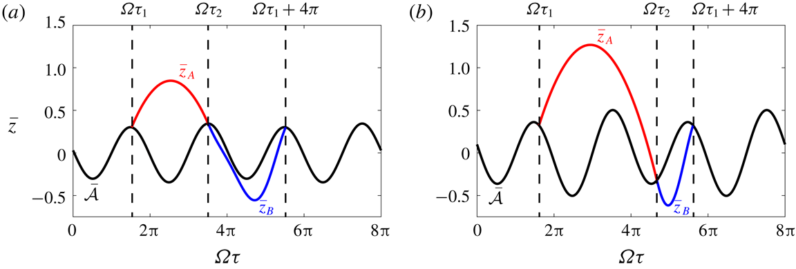
One period of the vertical displacement of a drop of radius
 $R=0.36$
mm predicted by the linear spring model in (a) a
 $(2,1)^{1}$
bouncing mode at
 $\unicode[STIX]{x1D6FE}=3g$
with local wave amplitude
 $\bar{h}_{p}=0.03$
, and (b) a
 $(2,1)^{2}$
bouncing mode at
 $\unicode[STIX]{x1D6FE}=4g$
with
 $\bar{h}_{p}=0.1$
, as viewed in the laboratory frame. The trajectories of the droplet in free flight,
 $z_{A}$
, and in contact with the bath,
 $z_{B}$
, are shown by the red and blue curves, respectively. The black curves denote the vertical position of the fluid surface,
 ${\mathcal{A}}$
, beneath the droplet.

To identify
 $(2,1)$
bouncing solutions, we seek periodic solutions to (4.2) with period
 $\unicode[STIX]{x1D70F}=4\unicode[STIX]{x03C0}/\unicode[STIX]{x1D6FA}$
where the droplet impacts the bath once during this period. Denoting the times at which the droplet leaves and hits the surface of the bath during a bouncing period by
 $\unicode[STIX]{x1D70F}_{1}$
and
 $\unicode[STIX]{x1D70F}_{2}$
, respectively, we require that
 $\bar{{\mathcal{Z}}}_{A}(\unicode[STIX]{x1D70F})$
and
 $\bar{{\mathcal{Z}}}_{B}(\unicode[STIX]{x1D70F})$
satisfy the following system of equations:
 $$\begin{eqnarray}\displaystyle \left.\begin{array}{@{}c@{}}\bar{{\mathcal{Z}}}_{A}(\unicode[STIX]{x1D70F}_{1})=0,\quad \bar{{\mathcal{Z}}}_{A}(\unicode[STIX]{x1D70F}_{2})=0,\quad \bar{{\mathcal{Z}}}_{B}(\unicode[STIX]{x1D70F}_{2})=0,\quad \bar{{\mathcal{Z}}}_{B}\left(\unicode[STIX]{x1D70F}_{1}+{\displaystyle \frac{4\unicode[STIX]{x03C0}}{\unicode[STIX]{x1D6FA}}}\right)=0,\\ \dot{\bar{{\mathcal{Z}}}}_{A}(\unicode[STIX]{x1D70F}_{2})=\dot{\bar{{\mathcal{Z}}}}_{B}(\unicode[STIX]{x1D70F}_{2}),\quad \dot{\bar{{\mathcal{Z}}}}_{A}(\unicode[STIX]{x1D70F}_{1})=\dot{\bar{{\mathcal{Z}}}}_{B}\left(\unicode[STIX]{x1D70F}_{1}+{\displaystyle \frac{4\unicode[STIX]{x03C0}}{\unicode[STIX]{x1D6FA}}}\right).\end{array}\right\} & & \displaystyle\end{eqnarray}$$
These conditions ensure that the drop’s vertical position and speed are continuous as it enters and leaves the bath, and that the bouncing motion has a period of
 $\unicode[STIX]{x1D70F}=4\unicode[STIX]{x03C0}/\unicode[STIX]{x1D6FA}$
. For given values of
 $\unicode[STIX]{x1D6FE}$
,
 $h_{p}$
, and
 $R$
, we can numerically solve the nonlinear system (4.5) to obtain
 $\unicode[STIX]{x1D70F}_{1}$
,
 $\unicode[STIX]{x1D70F}_{2}$
,
 $A_{1}$
,
 $A_{2}$
,
 $B_{1}$
and
 $B_{2}$
. Figure 9 shows examples of the bouncing solutions so deduced for droplets in
 $(2,1)^{1}$
and
 $(2,1)^{2}$
modes.
The dependence of the phase parameters
 ${\mathcal{S}}$
and
 ${\mathcal{C}}$
on
 $\unicode[STIX]{x1D6E4}=\unicode[STIX]{x1D6FE}/g$
and
 $\bar{h}_{p}=h_{p}/R$
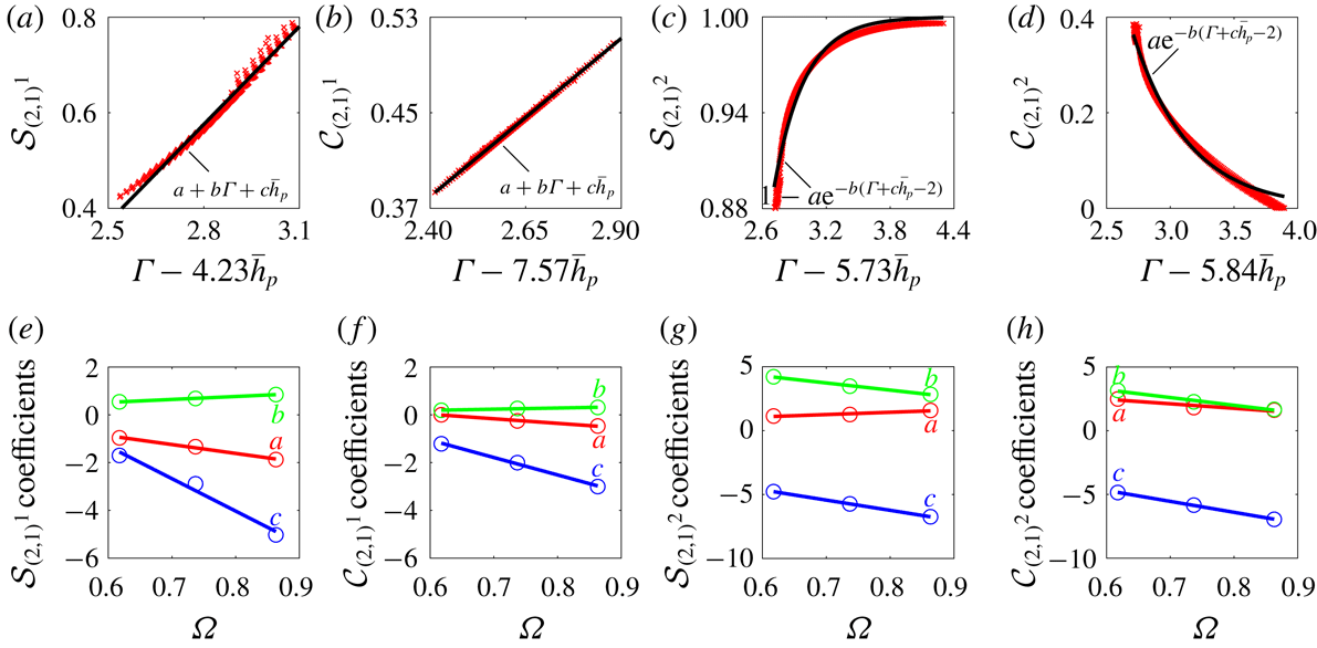
for a drop of radius
 $R=0.36$
mm in (a,b) the
 $(2,1)^{1}$
mode and (c,d) the
 $(2,1)^{2}$
mode. The red crosses are the values of the phase parameters obtained using the linear spring model and the black curves indicate approximate functional forms. Panels (e–h) show the dependencies of the coefficients for the functional forms in (a–d) on the non-dimensional drop radius
 $\unicode[STIX]{x1D6FA}$
. Lines of best fit are shown for reference.

For a given drop radius
 $R$
, we can then determine the regions in the
 $(\unicode[STIX]{x1D6FE},h_{p})$
-plane where
 $(2,1)^{1}$
and
 $(2,1)^{2}$
bouncing solutions exist, and compute the corresponding values of the phase parameters
 ${\mathcal{S}}$
and
 ${\mathcal{C}}$
. We thus obtain surfaces for
 ${\mathcal{S}}$
and
 ${\mathcal{C}}$
as functions of
 $\unicode[STIX]{x1D6FE}$
and
 $h_{p}$
. Next, we observe that each of these surfaces can be collapsed onto a curve by expressing
 ${\mathcal{S}}$
and
 ${\mathcal{C}}$
as functions of a new variable, a suitable linear combination of
 $\unicode[STIX]{x1D6FE}$
and
 $h_{p}$
. Examples of these collapses for
 $R=0.36$
mm are shown in figure 10(a–d), where the linear combination that best collapses the data is indicated on each
 $x$
-axis. We observe that for
 ${\mathcal{S}}$
and
 ${\mathcal{C}}$
in the
 $(2,1)^{1}$
mode, the data are both well approximated by linear relations, the coefficients extracted from a least squares fit. For
 ${\mathcal{S}}$
in the
 $(2,1)^{2}$
mode, we chose to fit the data with an exponential curve that asymptotes to one at high memories, as this is the maximum value that
 ${\mathcal{S}}$
can theoretically attain. Similarly, for
 ${\mathcal{C}}$
in the
 $(2,1)^{2}$
mode, we fit the data with an exponential curve that asymptotes to zero at high memories, on the grounds that we do not expect
 ${\mathcal{C}}$
to become negative, as would correspond to a reversal in walking direction. The same analysis is then repeated for drops of sizes
 $R=0.32$
mm and
 $R=0.40$
mm, and the dependencies of the function coefficients
 $a$
,
 $b$
and
 $c$
on the non-dimensional drop size
 $\unicode[STIX]{x1D6FA}$
are presented in figure 10(e–h). We see that the dependencies of the coefficients on
 $\unicode[STIX]{x1D6FA}$
are well approximated by linear functions. Based on the data in figure 10, we are able to develop functional forms for
 ${\mathcal{S}}$
and
 ${\mathcal{C}}$
, which depend on
 $\unicode[STIX]{x1D6FE}$
,
 $h_{p}$
and
 $R$
, as presented in table 2.
Approximate functional dependences of the phase parameters
 ${\mathcal{S}}$
and
 ${\mathcal{C}}$
on the non-dimensional driving acceleration of the bath,
 $\unicode[STIX]{x1D6E4}$
, the local wave amplitude,
 $\bar{h}_{p}$
, and the dimensionless drop radius,
 $\unicode[STIX]{x1D6FA}$
, for drops in a
 $(2,1)^{1}$
or
 $(2,1)^{2}$
bouncing mode. These relations are valid across the range of drop radii
 $0.6\leqslant \unicode[STIX]{x1D6FA}\leqslant 0.9$
considered in this study.

The relations for
 ${\mathcal{S}}$
and
 ${\mathcal{C}}$
given in table 2 were developed by considering a horizontally stationary bouncing droplet. They are also expected to be valid for walking drops provided that changes in
 $\unicode[STIX]{x1D6FE}$
and
 $h_{p}$
occur slowly relative to the bouncing period,
 $T_{F}$
, in which case the droplet’s vertical dynamics will closely resemble that of a stable bouncing state. Specifically, for fixed
 $\unicode[STIX]{x1D6FE}$
, we require that the time scale of bouncing,
 $T_{F}$
, be small relative to that over which the local wave amplitude changes by a characteristic value
 $\unicode[STIX]{x0394}h$
,
 $T_{h_{p}}=\unicode[STIX]{x0394}h/[(\unicode[STIX]{x2202}h_{p}/\unicode[STIX]{x2202}x)|\dot{\boldsymbol{x}}_{p}|]$
. In a typical experiment,
 $\unicode[STIX]{x2202}h_{p}/\unicode[STIX]{x2202}x\approx \unicode[STIX]{x0394}h/\unicode[STIX]{x1D706}_{F}$
and
 $|\dot{\boldsymbol{x}}_{p}|\approx 10~\text{mm}~\text{s}^{-1}$
which yields
 $T_{h_{p}}/T_{F}\approx 20\gg 1$
.
The strobed trajectory equation (2.9) coupled with the functions
 ${\mathcal{S}}={\mathcal{S}}(\unicode[STIX]{x1D6E4},\bar{h}_{p},\unicode[STIX]{x1D6FA})$
and
 ${\mathcal{C}}={\mathcal{C}}(\unicode[STIX]{x1D6E4},\bar{h}_{p},\unicode[STIX]{x1D6FA})$
presented in table 2, can now be used to compute the horizontal trajectory of a
 $(2,1)$
walker while simultaneously accounting for variations in the drop’s vertical dynamics. Except when modelling simple scenarios, such as single bouncers or straight-line walkers in unbounded geometries, incorporation of the influence of impact phase variations requires that the trajectory equation be solved numerically. Specifically, one must first discretize equation (2.9) using a numerical time-stepping scheme. At each time step, the wave amplitude at the position of the drop,
 $h_{p}$
, must be computed in order to obtain values for
 ${\mathcal{S}}$
and
 ${\mathcal{C}}$
, after which the drop’s horizontal position can be updated via the trajectory equation (2.9).
4.1 Impact-phase variations for single drops
We proceed by calculating how
 ${\mathcal{S}}$
and
 ${\mathcal{C}}$
vary with
 $\unicode[STIX]{x1D6FE}$
for single bouncers and straight-line walkers, in order to compare the predictions of our theoretical models for
 ${\mathcal{S}}$
and
 ${\mathcal{C}}$
with our experimental results in figure 4. According to the trajectory equation (2.9), the following equations must be satisfied for a single drop walking in a straight line with constant speed
 $u$
:
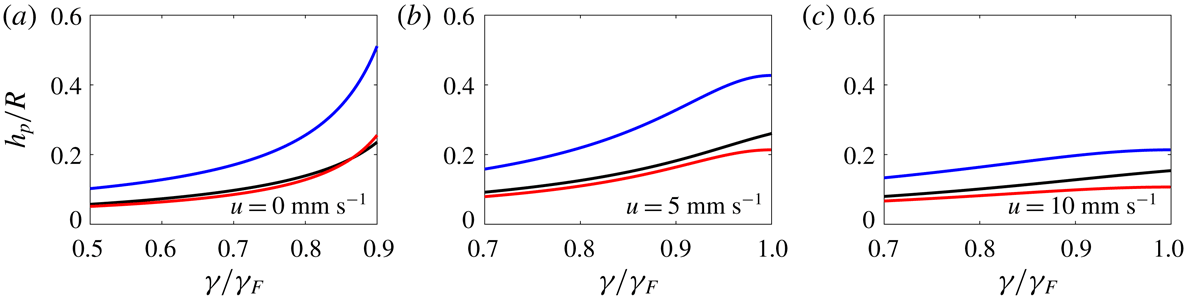
 $$\begin{eqnarray}\bar{h}_{p}={\displaystyle \frac{AM_{e}{\mathcal{S}}(\unicode[STIX]{x1D6E4},\bar{h}_{p},\unicode[STIX]{x1D6FA})}{R\sqrt{1+\bar{u}^{2}}}},\end{eqnarray}$$
 $$\begin{eqnarray}\bar{u}=\sqrt{\unicode[STIX]{x1D719}-{\displaystyle \frac{1}{2}}(1+\sqrt{1+4\unicode[STIX]{x1D719}})},\quad \unicode[STIX]{x1D719}={\displaystyle \frac{AM_{e}\unicode[STIX]{x1D6FD}{\mathcal{S}}(\unicode[STIX]{x1D6E4},\bar{h}_{p},\unicode[STIX]{x1D6FA}){\mathcal{C}}(\unicode[STIX]{x1D6E4},\bar{h}_{p},\unicode[STIX]{x1D6FA})}{R}}.\end{eqnarray}$$
 $R$
, the walking threshold,
 $\unicode[STIX]{x1D6FE}_{W}$
, is obtained by finding the value of
 $\unicode[STIX]{x1D6FE}$
that satisfies both
 $\unicode[STIX]{x1D719}=2$
and (4.6a
) with
 $\bar{u}=0$
. To compute the phase parameters for a bouncer, at a given value of
 $\unicode[STIX]{x1D6FE}$
, we first solve equation (4.6a
) for
 $\bar{h}_{p}$
, setting
 $\bar{u}=0$
. Knowing
 $\bar{h}_{p}$
then allows for
 ${\mathcal{S}}$
and
 ${\mathcal{C}}$
to be computed. In the case of a walker, we first solve the system of (4.6a
) and (4.6b
) in order to obtain
 $\bar{u}$
and
 $\bar{h}_{p}$
. From
 $\bar{h}_{p}$
, we can then compute
 ${\mathcal{S}}$
and
 ${\mathcal{C}}$
.
In figure 4, we compare our theoretical predictions for
 ${\mathcal{S}}$
and
 ${\mathcal{C}}$
with our experimental data. For values of
 $\unicode[STIX]{x1D6FE}$
where
 $(2,2)$
and
 $(4,2)$
modes were experimentally observed, we used our phase relations for
 $(2,1)^{1}$
and
 $(2,1)^{2}$
modes, respectively, as an approximation. Our model is seen to capture all of the observed trends in
 ${\mathcal{S}}$
and
 ${\mathcal{C}}$
, however, there is a horizontal shift between our experimental and theoretical data for the phase parameter
 ${\mathcal{S}}$
in the
 $(2,1)^{1}$
mode. This shift is a result of slight differences in the profile of the contact force,
 $F_{N}(t)$
, observed experimentally and predicted theoretically by the linear spring model. In particular,
 ${\mathcal{S}}$
is highly sensitive to the relative heights of the two maxima in
 $F_{N}(t)$
in the
 $(2,1)^{1}$
mode seen in figure 3, while
 ${\mathcal{C}}$
is not.
In figure 4(c), we compare our experimental data of walking thresholds and speeds for single drops with the theoretical predictions of both the constant-impact-phase model of Oza et al. (Reference Oza, Rosales and Bush2013) and the variable-phase model developed in this study. Oza et al. (Reference Oza, Rosales and Bush2013) used a fixed value of
 $\sin (\unicode[STIX]{x1D6F7})/2={\mathcal{S}}{\mathcal{C}}=0.30$
, chosen to best match the dependence of the walking speed on
 $\unicode[STIX]{x1D6FE}$
for a drop of radius
 $R=0.40$
mm. As seen in figure 4(c), this assumption of constant-impact-phase results in significant discrepancies between the theoretical predictions and experimental data for other drop sizes. By capturing the dependence of
 ${\mathcal{S}}$
and
 ${\mathcal{C}}$
on
 $R$
and
 $\unicode[STIX]{x1D6FE}$
, our model is able to adequately predict the walking thresholds across a range of drop sizes,
 $R=0.32$
, 0.36 and 0.40 mm. We note that for a drop radius of
 $R=0.36$
mm, the predicted walking speed at the walking threshold is non-zero, as the walking threshold occurs at the locus of the
 $(2,1)^{1}$
to
 $(2,1)^{2}$
transition, where the phase parameters change discontinuously. We also note that the model of Oza et al. (Reference Oza, Rosales and Bush2013) significantly over-predicts the experimentally measured walking speeds as
 $\unicode[STIX]{x1D6FE}/\unicode[STIX]{x1D6FE}_{F}$
approaches 1. By capturing the decrease in
 ${\mathcal{C}}$
with increasing
 $\unicode[STIX]{x1D6FE}$
in the
 $(2,1)^{2}$
mode, our variable-phase model is able to better capture the experimentally observed plateau in walking speeds at high memories. As shown in figure 12 in appendix A, our wave model underpredicts the local wave amplitude,
 $h_{p}$
, for fast walkers at high memories, compared to the model of Moláček & Bush (Reference Moláček and Bush2013b
) which is in agreement with experimental wavefield measurements. This results in the slight decrease in the theoretically predicted walking speed with increasing
 $\unicode[STIX]{x1D6FE}$
that is evident in figure 4(c) for a drop of radius
 $R=0.40$
mm.
4.2 Impact-phase variations for multiple drops
When modelling droplet–droplet interactions, it is necessary to use a wave model that accurately captures the far-field decay of the waves. Damiano et al. (Reference Damiano, Brun, Harris, Galeano-Rios and Bush2016), Tadrist et al. (Reference Tadrist, Shim, Gilet and Schlagheck2018b
) and Turton et al. (Reference Turton, Couchman and Bush2018) all proposed the inclusion of a spatio-temporal damping factor which modifies the wave kernel in (2.10) to an expression of the form
 $J_{0}(k_{F}|\boldsymbol{x}-\boldsymbol{x}_{p}(s)|)\exp \{-\unicode[STIX]{x1D6FC}|\boldsymbol{x}-\boldsymbol{x}_{p}(s)|^{2}/(t-s)\}$
. However, this factor is derived using a long-time asymptotic expansion that introduces an unphysical singularity in the second spatial derivative at
 $|\boldsymbol{x}-\boldsymbol{x}_{p}(s)|=0$
. The presence of this singularity greatly complicates a stability analysis of the trajectory equation (2.9). In order to analyse the stability of orbiting pairs, Oza et al. (Reference Oza, Siéfert, Harris, Moláček and Bush2017) modified this damping factor by setting
 $(t-s)\rightarrow (t-s+T_{F})$
. In their study of promenading pairs, Arbelaiz et al. (Reference Arbelaiz, Oza and Bush2018) neglected the spatio-temporal damping factor altogether. To eliminate these mathematical difficulties, in appendix B we use a quasi-static approximation to derive a purely spatial damping factor that is smooth at
 $|\boldsymbol{x}-\boldsymbol{x}_{p}(s)|=0$
, while remaining consistent with the spatio-temporal damping factor of Turton et al. (Reference Turton, Couchman and Bush2018) in the far field.
Based on (2.9), the equations governing a system of
 $N$
interacting drops are
 $$\begin{eqnarray}\unicode[STIX]{x1D705}\ddot{\bar{\boldsymbol{x}}}_{i}+\dot{\bar{\boldsymbol{x}}}_{i}=-\unicode[STIX]{x1D6FD}\unicode[STIX]{x1D70E}_{i}{\mathcal{C}}_{i}\unicode[STIX]{x1D735}\bar{h}(\bar{\boldsymbol{x}}_{i},\bar{t}),\quad i=1,2,\ldots ,N,\end{eqnarray}$$
where
 $$\begin{eqnarray}\bar{h}(\bar{\boldsymbol{x}},\bar{t})={\displaystyle \frac{AM_{e}}{R}}\mathop{\sum }_{j=1}^{N}\unicode[STIX]{x1D70E}_{j}\displaystyle \displaystyle \int _{-\infty }^{\bar{t}}{\mathcal{S}}_{j}f(|\bar{\boldsymbol{x}}-\bar{\boldsymbol{x}}_{j}(\bar{s})|)\text{e}^{-(\bar{t}-\bar{s})}\,\text{d}\bar{s}\end{eqnarray}$$
and the wave kernel, with the spatial damping factor derived in appendix B, is
 $$\begin{eqnarray}f(\bar{r})=J_{0}(\bar{r})[1+(\unicode[STIX]{x1D709}K_{1}(\unicode[STIX]{x1D709}\bar{r})\bar{r}-1)\text{e}^{-\bar{r}^{-2}}],\end{eqnarray}$$
where
 $\unicode[STIX]{x1D709}$
is defined in table 1. As a
 $(2,1)$
drop can either impact the bath during the first or second cycle of the bath’s oscillation, the parameters
 $\unicode[STIX]{x1D70E}_{i}=\pm 1$
are chosen to describe the relative bouncing phase of the drops:
 $\unicode[STIX]{x1D70E}_{i}\unicode[STIX]{x1D70E}_{j}=1$
and
 $\unicode[STIX]{x1D70E}_{i}\unicode[STIX]{x1D70E}_{j}=-1$
indicate that drops
 $i$
and
 $j$
are bouncing in-phase and out-of-phase, respectively. The phase parameters
 ${\mathcal{S}}_{i}$
and
 ${\mathcal{C}}_{i}$
describe modulations in the bouncing phase of the
 $i$
th drop within a given bath cycle.
The trajectory equation (4.7) highlights two main mechanisms through which droplets interact. Firstly, the gradient of the strobed wavefield,
 $\unicode[STIX]{x1D735}h$
, beneath a drop is altered due to waves generated by neighbouring drops. Secondly, neighbouring drops also alter the local wave amplitude beneath a drop,
 $h_{p}$
, which will change the drop’s vertical dynamics and hence
 ${\mathcal{S}}$
and
 ${\mathcal{C}}$
. This second interaction mechanism is not captured by a constant phase model but can significantly affect droplet–droplet interactions as we shall demonstrate in our analysis of the stability of droplet pairs.
4.3 Stability of bound droplet pairs
We analyse the stability of a bound pair of identical droplets using the system of (4.7). Pairs will exist in stationary bound states when the right-hand sides of (4.7) are zero, corresponding to the discrete set of separation distances,
 $d_{n}$
, that satisfy
 $f^{\prime }(d_{n})=0$
. In order for a separation distance
 $d_{n}$
to be stable, it must correspond to each drop bouncing in a minimum of its neighbour’s wavefield (Eddi et al.
Reference Eddi, Decelle, Fort and Couder2009). Thus, for drop’s bouncing in-phase
 $(\unicode[STIX]{x1D70E}_{1}\unicode[STIX]{x1D70E}_{2}=1)$
or out-of-phase
 $(\unicode[STIX]{x1D70E}_{1}\unicode[STIX]{x1D70E}_{2}=-1)$
, the stable separation distances correspond to the minima or maxima of
 $f(r)$
, respectively. In figure 5, we plot our theoretical predictions for stable values of
 $d_{n}$
at two values of
 $\unicode[STIX]{x1D6FE}$
, the bouncing threshold,
 $\unicode[STIX]{x1D6FE}_{B}$
, and the walking threshold,
 $\unicode[STIX]{x1D6FE}_{W}$
, of an individual drop. The values of
 $d_{n}$
are dependent on the vertical bouncing mode of the drops, as
 $(1,1)$
and
 $(2,1)$
drops excite waves of different wavelengths. Using the deep water dispersion relation for gravity–capillary waves,
 $\unicode[STIX]{x1D714}^{2}=gk+\unicode[STIX]{x1D70E}k^{3}/\unicode[STIX]{x1D70C}$
, we expect the wavelengths of the wavefields produced by
 $(1,1)$
and
 $(2,1)$
bouncers to be
 $\unicode[STIX]{x1D706}_{(1,1)}=2.86$
mm and
 $\unicode[STIX]{x1D706}_{(2,1)}=\unicode[STIX]{x1D706}_{F}=4.75$
mm, respectively. For the
 $(1,1)$
pairs in the vicinity of
 $\unicode[STIX]{x1D6FE}_{B}$
, our theoretical predictions for
 $d_{n}$
are found to be in good agreement with our experimental data, except at the high binding numbers
 $n=10$
and 11. This discrepancy presumably arises because the drop–drop interaction is so weak at such low
 $\unicode[STIX]{x1D6FE}$
and large
 $n$
that the drops had not fully settled into their equilibrium separation distances. For the
 $(2,1)$
pairs in the vicinity of
 $\unicode[STIX]{x1D6FE}_{W}$
, theoretical predictions are again found to be in good agreement with the experimental data, but slightly underpredict the experimental values of
 $d_{n}$
at small
 $n$
. One expects this slight discrepancy to be caused by the travelling wave fronts generated at each impact, an effect detailed by Galeano-Rios et al. (Reference Galeano-Rios, Couchman, Caldairou and Bush2018) that is not captured by the wave model (4.8).
Next, we examine how stationary
 $(2,1)$
bound pairs destabilize into horizontal motion as
 $\unicode[STIX]{x1D6FE}$
is increased. We assume that the drops start at stable positions
 $(x_{1},y_{1})=(0,0)$
and
 $(x_{2},y_{2})=(d_{n},0)$
and introduce arbitrary horizontal perturbations
 $x_{1}=\unicode[STIX]{x1D716}\unicode[STIX]{x1D6FF}x_{1}$
,
 $y_{1}=\unicode[STIX]{x1D716}\unicode[STIX]{x1D6FF}y_{1}$
,
 $x_{2}=d_{n}+\unicode[STIX]{x1D716}\unicode[STIX]{x1D6FF}x_{2}$
,
 $y_{2}=\unicode[STIX]{x1D716}\unicode[STIX]{x1D6FF}y_{2}$
. As shown in appendix C, substituting these perturbations into (4.7) and retaining only terms up to
 $O(\unicode[STIX]{x1D716})$
yields the following
 $12\times 12$
block diagonal, linear system:
 $$\begin{eqnarray}{\displaystyle \frac{\text{d}\unicode[STIX]{x1D64C}}{\text{d}t}}=\left[\begin{array}{@{}cccc@{}}\unicode[STIX]{x1D63C}_{3\times 3} & \mathbf{0} & \mathbf{0} & \mathbf{0}\\ \mathbf{0} & \unicode[STIX]{x1D63D}_{3\times 3} & \mathbf{0} & \mathbf{0}\\ \mathbf{0} & \mathbf{0} & \unicode[STIX]{x1D63E}_{3\times 3} & \mathbf{0}\\ \mathbf{0} & \mathbf{0} & \mathbf{0} & \unicode[STIX]{x1D63E}_{3\times 3}\end{array}\right]\unicode[STIX]{x1D64C},\end{eqnarray}$$
where
 $$\begin{eqnarray}\displaystyle \unicode[STIX]{x1D64C} & = & \displaystyle \big(\unicode[STIX]{x1D6FF}x_{1}+\unicode[STIX]{x1D6FF}x_{2},\unicode[STIX]{x1D6FF}u_{1}+\unicode[STIX]{x1D6FF}u_{2},\unicode[STIX]{x1D6FF}X_{1}+\unicode[STIX]{x1D6FF}X_{2},\unicode[STIX]{x1D6FF}x_{2}-\unicode[STIX]{x1D6FF}x_{1},\unicode[STIX]{x1D6FF}u_{2}-\unicode[STIX]{x1D6FF}u_{1},\unicode[STIX]{x1D6FF}X_{2}-\unicode[STIX]{x1D6FF}X_{1},\nonumber\\ \displaystyle & & \displaystyle \unicode[STIX]{x1D6FF}y_{1},\unicode[STIX]{x1D6FF}v_{1},\unicode[STIX]{x1D6FF}Y_{1},\unicode[STIX]{x1D6FF}y_{2},\unicode[STIX]{x1D6FF}v_{2},\unicode[STIX]{x1D6FF}Y_{2}\big),\end{eqnarray}$$
 $$\begin{eqnarray}\displaystyle \unicode[STIX]{x1D63C} & = & \displaystyle \left[\begin{array}{@{}ccc@{}}0 & 1 & 0\\ -\unicode[STIX]{x1D712}-\unicode[STIX]{x1D713} & -{\displaystyle \frac{1}{\unicode[STIX]{x1D705}}} & \unicode[STIX]{x1D712}+\unicode[STIX]{x1D713}\\ 1 & 0 & -1\end{array}\right],\quad \unicode[STIX]{x1D63D}=\left[\begin{array}{@{}ccc@{}}0 & 1 & 0\\ -\unicode[STIX]{x1D712}-\unicode[STIX]{x1D713} & -{\displaystyle \frac{1}{\unicode[STIX]{x1D705}}} & \unicode[STIX]{x1D712}-\unicode[STIX]{x1D713}\\ 1 & 0 & -1\end{array}\right],\nonumber\\ \displaystyle & & \displaystyle \qquad \unicode[STIX]{x1D63E}=\left[\begin{array}{@{}ccc@{}}0 & 1 & 0\\ -\unicode[STIX]{x1D712} & -{\displaystyle \frac{1}{\unicode[STIX]{x1D705}}} & \unicode[STIX]{x1D712}\\ 1 & 0 & -1\end{array}\right],\end{eqnarray}$$
 $$\begin{eqnarray}\unicode[STIX]{x1D712}={\displaystyle \frac{AM_{e}\unicode[STIX]{x1D6FD}{\mathcal{C}}_{n}{\mathcal{S}}_{n}}{R\unicode[STIX]{x1D705}}}f^{\prime \prime }(0),\quad \unicode[STIX]{x1D713}={\displaystyle \frac{AM_{e}\unicode[STIX]{x1D6FD}{\mathcal{C}}_{n}{\mathcal{S}}_{n}}{R\unicode[STIX]{x1D705}}}\unicode[STIX]{x1D70E}_{1}\unicode[STIX]{x1D70E}_{2}f^{\prime \prime }(\bar{d}_{n}).\end{eqnarray}$$
The effect of the vertical dynamics on the pair’s horizontal stability is captured by
 ${\mathcal{S}}_{n}$
and
 ${\mathcal{C}}_{n}$
, which are the values of the phase parameters for each drop in an initially horizontally static pair with separation distance
 $d_{n}$
. Following the same procedure as in § 4.1,
 ${\mathcal{S}}_{n}$
and
 ${\mathcal{C}}_{n}$
can be found by solving the implicit equation (4.8) for the local wave amplitude,
 $\bar{h}_{p}$
:
 $$\begin{eqnarray}\bar{h}_{p}={\displaystyle \frac{AM_{e}{\mathcal{S}}(\unicode[STIX]{x1D6E4},\bar{h}_{p},\unicode[STIX]{x1D6FA})}{R}}(1+\unicode[STIX]{x1D70E}_{1}\unicode[STIX]{x1D70E}_{2}f(\bar{d}_{n})).\end{eqnarray}$$
Having obtained
 $\bar{h}_{p}$
for a given separation distance
 $\bar{d}_{n}$
, the corresponding values of
 ${\mathcal{S}}_{n}$
and
 ${\mathcal{C}}_{n}$
can be obtained using the relations in table 2.
In figure 6, we compare our theoretical predictions for
 ${\mathcal{S}}_{n}$
and
 ${\mathcal{C}}_{n}$
with our experimental data for pairs of radius
 $R=0.32$
mm and 0.40 mm with binding numbers
 $n=1$
and 2. Both our theoretical model and experimental data highlight important features of the phase parameters close to the pair instability thresholds. The pairs of radius
 $R=0.40$
mm are in a
 $(2,1)^{1}$
bouncing mode and both
 ${\mathcal{S}}_{n}$
and
 ${\mathcal{C}}_{n}$
increase with decreasing
 $n$
. Conversely, the pairs of radius
 $R=0.32$
mm are in a
 $(2,1)^{2}$
bouncing mode and while
 ${\mathcal{S}}$
has saturated to 1 for all
 $n$
,
 ${\mathcal{C}}$
now decreases with decreasing
 $n$
. We proceed by demonstrating that this subtle difference in the dependences of
 ${\mathcal{S}}$
and
 ${\mathcal{C}}$
on
 $n$
has a dramatic effect on a pair’s horizontal stability.
The block diagonal matrix in (4.10) indicates that there are three ways in which a pair of initially stationary drops may destabilize into horizontal motion. The sub-matrix
 $\unicode[STIX]{x1D63C}$
governs the stability of the quantity
 $\unicode[STIX]{x1D6FF}x_{1}+\unicode[STIX]{x1D6FF}x_{2}$
which corresponds to motion of the pair’s centre of mass in the
 $\hat{\unicode[STIX]{x1D66D}}$
-direction. All of the eigenvalues of
 $\unicode[STIX]{x1D63C}$
are real and one is zero, indicating that the pair is invariant to changes in the
 $\hat{\unicode[STIX]{x1D66D}}$
position of its centre of mass. As
 $\unicode[STIX]{x1D6FE}$
is increased across the instability threshold
 $\unicode[STIX]{x1D6FE}_{\ast }$
, the two non-zero eigenvalues switch from both being negative, to one being negative and the other positive. The resulting instability corresponds to a translation of the pair’s centre of mass in the
 $\hat{\boldsymbol{x}}$
-direction, where one drop follows the other while the inter-drop spacing,
 $d$
, remains fixed. We refer to this instability as a co-linear translation.
The sub-matrix
 $\unicode[STIX]{x1D63D}$
governs the stability of the quantity
 $\unicode[STIX]{x1D6FF}x_{2}-\unicode[STIX]{x1D6FF}x_{1}$
, which corresponds to changes in the inter-drop distance,
 $d$
.
 $\unicode[STIX]{x1D63D}$
has a real eigenvalue and a pair of complex conjugate eigenvalues. As
 $\unicode[STIX]{x1D6FE}$
is increased across the instability threshold
 $\unicode[STIX]{x1D6FE}_{\ast }$
, the real eigenvalue remains negative, while the real parts of both complex conjugate eigenvalues switch from negative to positive. The resulting instability corresponds to co-linear oscillations in the
 $\hat{\boldsymbol{x}}$
-direction about a fixed centre of mass.
The theoretical instability thresholds,
 $\unicode[STIX]{x1D6FE}_{\ast }$
, for co-linear translations of the pair’s centre of mass (green, matrix
 $\unicode[STIX]{x1D63C}$
), co-linear oscillations (blue, matrix
 $\unicode[STIX]{x1D63D}$
) and transverse motion (red, matrix
 $\unicode[STIX]{x1D63E}$
) as a function of the pair’s initial separation distance,
 $d$
. The corresponding experimental data from figure 7 are indicated by the black circles. The panels illustrate predicted thresholds for (a)
 $R=0.40$
mm with a variable-phase model, (b)
 $R=0.40$
mm with a constant-phase model, (c)
 $R=0.32$
mm with a variable-phase model and (d)
 $R=0.32$
mm with a constant-phase model. The variable- and constant-phase models correspond to predictions based on the linear system (4.10) using the phase functions
 ${\mathcal{S}}$
and
 ${\mathcal{C}}$
listed in table 2, and the constant value of the phase parameter
 $\sin (\unicode[STIX]{x1D6F7})/2={\mathcal{S}}{\mathcal{C}}=0.30$
used by Oza et al. (Reference Oza, Rosales and Bush2013), respectively.
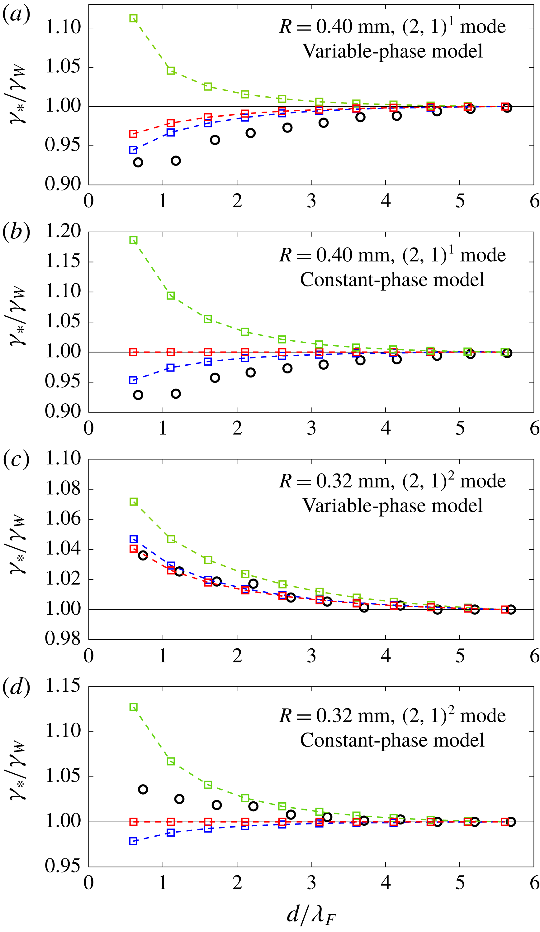
The sub-matrix
 $\unicode[STIX]{x1D63E}$
governs each drop’s stability to perturbations in the
 $\hat{\boldsymbol{y}}$
-direction, which we will refer to as transverse perturbations. The onset of orbital and promenading motion are both examples of such transverse instabilities. We note that
 $\unicode[STIX]{x1D63E}$
is exactly the matrix obtained by Oza et al. (Reference Oza, Rosales and Bush2013) that governs the bouncing to walking transition of a single droplet. As the linear system (4.10) predicts that the transverse perturbations of each drop in a pair are independent of the motion of the neighbouring droplet, it might seem that each drop will destabilize into walking in the
 $\hat{\boldsymbol{y}}$
-direction at
 $\unicode[STIX]{x1D6FE}_{W}$
, the walking threshold of an individual droplet. However, this is not the case: although the pairs do not interact through the gradient of each other’s wavefield, they modify each other’s local wave amplitude,
 $h_{p}$
, as captured by the phase parameters
 ${\mathcal{S}}$
and
 ${\mathcal{C}}$
. Therefore, for transverse perturbations, the droplets interact solely through modulations in their vertical dynamics, an effect that cannot be captured by a constant-impact-phase model.
In figure 11, we present the theoretical instability thresholds,
 $\unicode[STIX]{x1D6FE}_{\ast }$
, for co-linear translations of the pair’s centre of mass (matrix
 $\unicode[STIX]{x1D63C}$
), co-linear oscillations (matrix
 $\unicode[STIX]{x1D63D}$
) and transverse motions (matrix
 $\unicode[STIX]{x1D63E}$
) as a function of the pair’s initial separation distance,
 $d_{n}$
. We compare our experimental measurements from figure 7 to the theoretical predictions based on both our variable-impact-phase functions
 ${\mathcal{S}}$
and
 ${\mathcal{C}}$
listed in table 2, and the constant impact phase
 $\sin (\unicode[STIX]{x1D6F7})/2={\mathcal{S}}{\mathcal{C}}=0.30$
used by Oza et al. (Reference Oza, Rosales and Bush2013). For pairs in the
 $(2,1)^{2}$
mode, our variable-phase model predicts that the pairs destabilize above the walking threshold of an individual drop,
 $\unicode[STIX]{x1D6FE}_{W}$
, and that the most unstable motion is transverse, in agreement with our experiments. We note that for higher binding numbers
 $n$
, the instability thresholds for transverse motion and co-linear oscillations become progressively closer. This is consistent with our experimental observations that the promenading states begin to oscillate for
 $n>2.5$
. For pairs in the
 $(2,1)^{1}$
mode, our variable-phase model predicts that the pairs now destabilize below
 $\unicode[STIX]{x1D6FE}_{W}$
with the most unstable motion corresponding to co-linear oscillations, again in agreement with our experimental results.
Comparing the predictions of our variable-phase model with those of a constant-phase model makes clear that modulations in the vertical dynamics strongly affect the stability of droplet pairs. For example, a constant-phase model cannot predict the difference in behaviour between the
 $(2,1)^{1}$
and
 $(2,1)^{2}$
pairs: it predicts that both pair sizes should destabilize into co-linear oscillations below
 $\unicode[STIX]{x1D6FE}_{W}$
. The fact that
 $(2,1)^{1}$
and
 $(2,1)^{2}$
pairs destabilize below and above
 $\unicode[STIX]{x1D6FE}_{W}$
, respectively, is a direct consequence of the phase variations induced by the presence of a neighbouring drop. As the binding number,
 $n$
, of a pair decreases, so does the local wave amplitude beneath each drop,
 $h_{p}$
, as each drop sits in a deeper minimum of its neighbour’s wavefield. Based on table 2, we see that the phase parameters have opposite dependencies on
 $h_{p}$
for
 $(2,1)^{1}$
and
 $(2,1)^{2}$
drops. In the
 $(2,1)^{1}$
mode, both
 ${\mathcal{S}}$
and
 ${\mathcal{C}}$
increase with decreasing
 $h_{p}$
. Therefore, pairs with smaller binding numbers
 $n$
generate relatively large waves and receive relatively large horizontal impulses from the bath, prompting an onset of motion below
 $\unicode[STIX]{x1D6FE}_{W}$
. Conversely, for pairs in a
 $(2,1)^{2}$
mode,
 ${\mathcal{S}}$
has saturated to 1 while
 ${\mathcal{C}}$
now decreases with decreasing
 $h_{p}$
causing the drops to stabilize each other above
 $\unicode[STIX]{x1D6FE}_{W}$
.
5 Discussion
The trajectory equation (2.9), coupled with the impact phase functions
 ${\mathcal{S}}(\unicode[STIX]{x1D6E4},\bar{h}_{p},\unicode[STIX]{x1D6FA})$
and
 ${\mathcal{C}}(\unicode[STIX]{x1D6E4},\bar{h}_{p},\unicode[STIX]{x1D6FA})$
presented in table 2, provides a stroboscopic model for a drop’s horizontal motion that accounts for modulations in the drop’s vertical dynamics. Our model is valid for drops in the resonant
 $(2,1)$
bouncing mode, the regime of interest in the study of hydrodynamic quantum analogues. We have highlighted how variations in a drop’s vertical motion affect both the amplitude of the wave generated at each bounce, as described by
 ${\mathcal{S}}$
, as well as the horizontal impulse imparted on the drop by the bath, as described by
 ${\mathcal{C}}$
, quantities that strongly influence the drop’s horizontal motion.
Previous models for the horizontal motion of walking droplets can be categorized according to whether or not they account for variations in the vertical dynamics. Models that neglect such variations (Oza et al.
Reference Oza, Rosales and Bush2013; Bush et al.
Reference Bush, Oza and Moláček2014; Dubertrand et al.
Reference Dubertrand, Hubert, Schlagheck, Vandewalle, Bastin and Martin2016; Durey & Milewski Reference Durey and Milewski2017; Faria Reference Faria2017; Nachbin et al.
Reference Nachbin, Milewski and Bush2017) are easier to work with mathematically and have numerical simulation times comparable to, or faster than real time. However, they have limited predictive power in that a fitting parameter resulting from the unresolved vertical dynamics must be used to match experimental data. Conversely, models that explicitly simulate a drop’s coupled vertical and horizontal motion (Milewski et al.
Reference Milewski, Galeano-Rios, Nachbin and Bush2015; Galeano-Rios et al.
Reference Galeano-Rios, Milewski and Vanden-Broeck2017) have no such fitting parameter but are computationally intensive, with numerical simulations
 $10^{2}{-}10^{4}$
times slower than real time. The new model developed in this study bridges the gap between these two categories; specifically, it accounts for variations in a drop’s vertical dynamics while maintaining the simplicity of the stroboscopic models. Our model is particularly suited to examining the role played by the vertical dynamics in droplet chains (Filoux, Hubert & Vandewalle Reference Filoux, Hubert and Vandewalle2015) and lattices (Protière et al.
Reference Protière, Couder, Fort and Boudaoud2005; Lieber et al.
Reference Lieber, Hendershott, Pattanaporkratana and Maclennan2007; Eddi et al.
Reference Eddi, Terwagne, Fort and Couder2008, Reference Eddi, Decelle, Fort and Couder2009; Eddi, Boudaoud & Couder Reference Eddi, Boudaoud and Couder2011a
), systems that would require considerable amounts of computational power to perform full numerical simulations of each drop’s coupled horizontal and vertical motion.
For single bouncers and steady, rectilinear walkers in a homogeneous bath, the phase parameters are uniquely determined by
 $\unicode[STIX]{x1D6FE}$
and
 $R$
. As shown in figure 4, our model was able to adequately predict the experimentally measured dependences of
 ${\mathcal{S}}$
and
 ${\mathcal{C}}$
on
 $\unicode[STIX]{x1D6FE}$
for single bouncers and walkers of three different sizes across a range of driving accelerations spanning the
 $(2,1)$
mode. Based on these results, we can now justify why the majority of droplets begin to walk only once they have entered the
 $(2,1)^{2}$
mode, as shown in the regime diagram in figure 1. In order for a drop to walk, the wave amplitude must be sufficiently large to overcome the drag forces resisting horizontal motion (Moláček & Bush Reference Moláček and Bush2013b
). In the
 $(2,1)^{2}$
mode,
 ${\mathcal{S}}$
is close to one, meaning that at each bounce the droplet produces a wave of maximum possible amplitude, compared to a
 $(2,1)^{1}$
drop where
 ${\mathcal{S}}\approx 0.5$
and waves are only generated with
 ${\approx}50\,\%$
efficiency. Figure 4 also highlights the strong dependence of the phase parameters on the drop radius
 $R$
. This explains why both Moláček & Bush (Reference Moláček and Bush2013b
) and Oza et al. (Reference Oza, Rosales and Bush2013) could only successfully fit experimentally measured walking thresholds and speeds for one drop size, using a constant-phase model. By incorporating a variable phase, our model can now reproduce this experimental data across a range of drop sizes. We note that Moláček & Bush (Reference Moláček and Bush2013b
) used a value of
 $\sin (\unicode[STIX]{x1D6F7})/2={\mathcal{S}}{\mathcal{C}}=0.25$
to best fit the experimental data for a drop of size
 $R=0.40$
mm. In figure 4, the product
 ${\mathcal{S}}{\mathcal{C}}$
is seen to vary from approximately 0.35 to 0.2 for
 $R=0.40$
mm in the walking regime, explaining why Moláček & Bush (Reference Moláček and Bush2013b
) were able to obtain an adequate fit using a value of 0.25. Furthermore, using a constant-phase model, both Moláček & Bush (Reference Moláček and Bush2013b
) and Oza et al. (Reference Oza, Rosales and Bush2013) overpredicted the walking speeds at high memories. By capturing the decrease in
 ${\mathcal{C}}$
with increasing
 $\unicode[STIX]{x1D6FE}$
, our model now captures the experimentally observed plateau in walking speeds at high memories, as is evident in figure 4.
For systems containing multiple droplets, the phase parameters can change independently of
 $\unicode[STIX]{x1D6FE}$
and
 $R$
, as shown in figure 6, due to changes in the local wave amplitude induced by neighbouring drops. By characterizing how bound droplet pairs destabilize as
 $\unicode[STIX]{x1D6FE}$
is increased, we find that variations in the pair’s vertical dynamics strongly influence the nature of the droplet–droplet interaction. For example, figure 7 highlights that the interaction between droplet pairs in a
 $(2,1)^{1}$
bouncing mode promotes an onset of instability below the walking threshold,
 $\unicode[STIX]{x1D6FE}_{W}$
, of an individual drop. Conversely, the interaction between droplet pairs in a
 $(2,1)^{2}$
bouncing mode has the opposite effect, stabilizing the pair above
 $\unicode[STIX]{x1D6FE}_{W}$
. This difference in behaviour is due to variations in the pair’s impact phase. For
 $(2,1)^{1}$
bound pairs, both
 ${\mathcal{S}}$
and
 ${\mathcal{C}}$
increase with decreasing binding number
 $n$
which augments the strength of the droplet–droplet interaction and promotes instability. Conversely, for
 $(2,1)^{2}$
bound pairs,
 ${\mathcal{S}}\approx 1$
remains roughly constant while
 ${\mathcal{C}}$
decreases with decreasing
 $n$
, resulting in stabilization. As shown in figure 11, our variable-impact-phase model is able to capture both the type and thresholds of instability observed in our experiments, while a constant-impact-phase model is not. This distinction highlights the importance of accounting for phase variations when modelling systems containing multiple droplets.
Our study also allows us to better understand the results of the studies of Oza et al. (Reference Oza, Siéfert, Harris, Moláček and Bush2017) and Arbelaiz et al. (Reference Arbelaiz, Oza and Bush2018) on orbiting and promenading droplet pairs. In both studies, the walking speed of the pairs was observed to decrease below the free speed of an individual drop with decreasing binding number
 $n$
, prompting both studies to develop ad hoc empirical functions for
 $\sin (\unicode[STIX]{x1D6F7})/2={\mathcal{S}}{\mathcal{C}}$
that decreased with decreasing
 $n$
in order to fit their experimental data. Our study now rationalizes these trends in terms of the droplet pair’s variable vertical dynamics. For
 $(2,1)^{2}$
drops, the local wave amplitude and hence the phase parameter
 ${\mathcal{C}}$
decrease with decreasing
 $n$
, reducing the horizontal impulse the pair receives from the bath. We note that for drops in a
 $(2,1)^{1}$
mode, the opposite behaviour is expected on the basis of our study: the walking speed of the pair should increase with decreasing
 $n$
, thus exceeding the walking speed of a single drop. Accounting for a droplet’s vertical dynamics is also expected to be important when modelling a drop’s interaction with a submerged barrier. For example, Pucci et al. (Reference Pucci, Sáenz, Faria and Bush2016) observed experimentally that a walking droplet will slow down in the vicinity of a submerged barrier and Damiano et al. (Reference Damiano, Brun, Harris, Galeano-Rios and Bush2016) observed experimentally that the wavefield gets significantly damped in the vicinity of such a barrier. The results of our study could help link these two observations: for a
 $(2,1)^{2}$
walker, our model predicts that
 ${\mathcal{C}}$
and hence a drop’s walking speed will decrease when the local wave amplitude decreases, as one expects to arise in the vicinity of barriers.
Although our derivations of the phase functions
 ${\mathcal{S}}$
and
 ${\mathcal{C}}$
were restricted to drops in a
 $(2,1)$
bouncing mode, our analysis of the vertical dynamics can be readily extended to other modes. As shown in figure 4, our models of
 ${\mathcal{S}}$
and
 ${\mathcal{C}}$
for
 $(2,1)$
bouncers already seem to approximate well the experimentally observed impact phases in the neighbouring
 $(2,2)$
and
 $(4,2)$
regimes. Moreover, it would be relatively straightforward to develop phase functions for
 $(1,1)$
bouncers, for instance. First, the approximation
 $h_{p}=0$
could be used in (4.1) as the surface wave amplitude is negligible compared to the vibrational amplitude of the bath,
 $\unicode[STIX]{x1D6FE}/\unicode[STIX]{x1D714}^{2}$
, for the small values of
 $\unicode[STIX]{x1D6FE}$
for which
 $(1,1)$
bouncers exist. Then, a similar analysis to that presented in §4 could be performed, this time seeking periodic solutions to the linear spring model (4.2) with period
 $T_{F}/2$
. We also note that Tadrist et al. (Reference Tadrist, Sampara, Schlagheck and Gilet2018a
) have recently found that, in certain parameter regimes, two interacting droplets can suddenly flip their relative bouncing phases. In our model, the relative bouncing phases are prescribed through the parameters
 $\unicode[STIX]{x1D70E}_{i}=\pm 1$
in (4.7), and so cannot change in time. However, if a mechanism causing such reversals in bouncing phase were to be identified, it could be incorporated into (4.7).
When modelling multiple droplets, it may also be necessary to use a more complex wave model than that presented in (4.8). For instance, Galeano-Rios et al. (Reference Galeano-Rios, Couchman, Caldairou and Bush2018) found that travelling wave fronts have a significant influence on the horizontal motion of ratcheting pairs (Eddi et al. Reference Eddi, Terwagne, Fort and Couder2008). We note that the phase functions in table 2 are valid for any wave model in which the drop produces a standing wave at each impact that oscillates with half the frequency of the bath. To develop phase functions for a traveling wave model, the more complicated time dependence of the surface waves would first have to be incorporated into (4.1), after which the same analysis presented in this study could be followed.
Finally, a subject of current interest is the droplet–droplet correlations that may be induced by wave-mediated forces, such as drops communicating between one-dimensional slots (Nachbin Reference Nachbin2018) and in hydrodynamic spin lattices (Sáenz et al. Reference Sáenz, Pucci, Goujon, Cristea-Platon, Dunkel and Bush2018). As these correlations are expected to depend on the drop’s vertical dynamics, our model is likely to yield valuable insight into the interactions and statistical correlations emerging in these subtle multiple-drop systems.
Acknowledgements
M.M.P.C. gratefully acknowledges the financial support of the Natural Sciences and Engineering Research Council (NSERC) through grant no. 502891. J.W.M.B. gratefully acknowledges the financial support of the National Science Foundation (NSF) through grants DMS-1614043 and CMMI-1727565. We thank Professor R. R. Rosales for valuable discussions, and particularly his contribution to the theoretical developments in appendix B.
Appendix A. Wave-amplitude correction
We here compare the local wave amplitudes,
 $h_{p}$
, predicted by the discrete wave model of Moláček & Bush (Reference Moláček and Bush2013b
) (2.1) and the continuous wave model of Oza et al. (Reference Oza, Rosales and Bush2013) (2.8) for single bouncers and walkers. For a droplet walking with speed
 $u$
in a straight line, the model of Moláček & Bush (Reference Moláček and Bush2013b
) predicts that
 $$\begin{eqnarray}h_{p}=\sqrt{{\displaystyle \frac{2\unicode[STIX]{x1D708}_{e}}{\unicode[STIX]{x03C0}}}}{\displaystyle \frac{mgk_{F}^{3}R^{2}T_{F}}{\unicode[STIX]{x1D70E}(3k_{F}^{2}R^{2}+Bo)}}{\mathcal{S}}\mathop{\sum }_{n=1}^{\infty }{\displaystyle \frac{J_{0}(k_{F}unT_{F})}{\sqrt{nT_{F}}}}\text{e}^{-n/M_{e}},\end{eqnarray}$$
where the sum must be performed numerically. The model of Oza et al. (Reference Oza, Rosales and Bush2013) approximates the sum in the model of Moláček & Bush (Reference Moláček and Bush2013b
) by an integral which results in a different local wave amplitude for a droplet walking with speed
 $u$
:
 $$\begin{eqnarray}\displaystyle h_{p} & = & \displaystyle \sqrt{{\displaystyle \frac{2\unicode[STIX]{x1D708}_{e}}{\unicode[STIX]{x03C0}T_{F}}}}{\displaystyle \frac{mgk_{F}^{3}R^{2}}{\unicode[STIX]{x1D70E}(3k_{F}^{2}R^{2}+Bo)}}{\mathcal{S}}\displaystyle \displaystyle \int _{0}^{\infty }J_{0}(k_{F}uz)\text{e}^{-z/(T_{F}M_{e})}\,\text{d}z\end{eqnarray}$$
 $$\begin{eqnarray}\displaystyle & = & \displaystyle \sqrt{{\displaystyle \frac{2\unicode[STIX]{x1D708}_{e}}{\unicode[STIX]{x03C0}T_{F}}}}{\displaystyle \frac{mgk_{F}^{3}R^{2}}{\unicode[STIX]{x1D70E}(3k_{F}^{2}R^{2}+Bo)}}{\displaystyle \frac{T_{F}Me}{\sqrt{1+(k_{F}T_{F}M_{e}u)^{2}}}}{\mathcal{S}}.\end{eqnarray}$$
Figure 12 shows the dependence of
 $h_{p}$
on
 $\unicode[STIX]{x1D6FE}$
as predicted by the models of Moláček & Bush (Reference Moláček and Bush2013b
) (A 1) and Oza et al. (Reference Oza, Rosales and Bush2013) (A 3) for bouncers (
 $u=0$
) and walkers with prescribed speeds of
 $u=5$
and
 $10~\text{mm}~\text{s}^{-1}$
. In all cases, the wave amplitude of Oza et al. (Reference Oza, Rosales and Bush2013) is seen to overpredict that of Moláček & Bush (Reference Moláček and Bush2013b
). This discrepancy is due to the approximation of Oza et al. (Reference Oza, Rosales and Bush2013) to replace the
 $1/\sqrt{t}$
decay factor in the model of Moláček & Bush (Reference Moláček and Bush2013b
) by
 $1/\sqrt{T_{F}}$
, in order to avoid the singularity that would otherwise appear in the integral model at
 $t=0$
.
The non-dimensional local wave amplitude,
 $h_{p}/R$
, as a function of the non-dimensional driving acceleration,
 $\unicode[STIX]{x1D6FE}/\unicode[STIX]{x1D6FE}_{F}$
, for a drop of radius
 $R=0.36$
mm that is (a) bouncing, (b) walking at speed
 $u=5~\text{mm}~\text{s}^{-1}$
and (c) walking at speed
 $u=10~\text{mm}~\text{s}^{-1}$
. The black line corresponds to the discrete model of Moláček & Bush (Reference Moláček and Bush2013b
), the blue line to the continuous model of Oza et al. (Reference Oza, Rosales and Bush2013) and the red line to the model of Oza et al. (Reference Oza, Rosales and Bush2013) with the wave amplitude divided by 2, as used in this study to better approximate the model of Moláček & Bush (Reference Moláček and Bush2013b
);
 ${\mathcal{S}}=1$
has been used for the sake of comparison.

For a bouncer, one can calculate the factor needed to correct this discrepancy. Specifically, the local wave amplitudes predicted by the model of Moláček & Bush (Reference Moláček and Bush2013b
) (A 1) and Oza et al. (Reference Oza, Rosales and Bush2013) (A 3) differ by the factor
 $\text{Li}_{1/2}(\text{e}^{-1/M_{e}})/M_{e}$
, where
 $\text{Li}_{n}(x)$
denotes the polylogarithm function of order
 $n$
. However, for a walker, a different correction factor would be required that would depend not only on the memory,
 $M_{e}$
, but also on the walker’s speed,
 $u$
, and past trajectory. For example, the scaling factor would be different for a drop walking in a circle compared to a drop walking in a straight line. To more accurately approximate the discrete wave model of Moláček & Bush (Reference Moláček and Bush2013b
) using an integral would require the development of a non-singular model for the behaviour of the wavefield for times
 $t<T_{F}$
, immediately following a drop’s impact. This is beyond the scope of this paper which is focused on modelling the coupling between a drop’s vertical and horizontal dynamics. Instead, in figure 12 we observe that for both bouncers and walkers of various speeds across a range of memories, the integral model of Oza et al. (Reference Oza, Rosales and Bush2013) overpredicts
 $h_{p}$
by approximately a factor of two relative to the predictions of the discrete model of Moláček & Bush (Reference Moláček and Bush2013b
). Thus, in order to obtain a qualitative agreement between the wave amplitudes of Oza et al. (Reference Oza, Rosales and Bush2013) and Moláček & Bush (Reference Moláček and Bush2013b
), we proceed by dividing the wave amplitude of Oza et al. (Reference Oza, Rosales and Bush2013) by a factor of two.
Appendix B. Quasi-static spatial damping factor
We use a quasi-static approximation to derive a purely spatial damping factor that remains consistent with the spatio-temporal damping factor proposed by Turton et al. (Reference Turton, Couchman and Bush2018) but that is smooth at the origin. Including the spatio-temporal damping factor of Turton et al. (Reference Turton, Couchman and Bush2018) in the wave model (2.10) yields
 $$\begin{eqnarray}h(\boldsymbol{x},t)={\displaystyle \frac{A}{T_{F}}}\displaystyle \displaystyle \int _{-\infty }^{t}{\mathcal{S}}f(|\boldsymbol{x}-\boldsymbol{x}_{p}(s)|,t-s)\text{e}^{-(t-s)/(T_{F}M_{e})}\,\text{d}s,\end{eqnarray}$$
where
 $$\begin{eqnarray}f(r,t)=J_{0}(k_{F}r)\text{e}^{-\unicode[STIX]{x1D6FC}r^{2}/t},\end{eqnarray}$$
and
 $\unicode[STIX]{x1D6FC}$
is defined in table 1.
Consider the wavefield produced by a drop bouncing in place at the position
 $\boldsymbol{x}_{p}=0$
:
 $$\begin{eqnarray}\displaystyle h_{B}(|\boldsymbol{x}|) & = & \displaystyle {\displaystyle \frac{A{\mathcal{S}}}{T_{F}}}J_{0}(k_{F}|\boldsymbol{x}|)\displaystyle \displaystyle \int _{0}^{\infty }\text{e}^{-\unicode[STIX]{x1D6FC}|\boldsymbol{x}|^{2}/z-z/(T_{F}M_{e})}\,\text{d}z\end{eqnarray}$$
 $$\begin{eqnarray}\displaystyle & = & \displaystyle 2A{\mathcal{S}}\sqrt{{\displaystyle \frac{\unicode[STIX]{x1D6FC}M_{e}}{T_{F}}}}J_{0}(k_{F}|\boldsymbol{x}|)K_{1}\left(2\sqrt{{\displaystyle \frac{\unicode[STIX]{x1D6FC}}{T_{F}M_{e}}}}|\boldsymbol{x}|\right)|\boldsymbol{x}|.\end{eqnarray}$$
We note that the integrand in (B 3) is sharply peaked around
 $z=|\boldsymbol{x}|\sqrt{\unicode[STIX]{x1D6FC}T_{F}M_{e}}$
meaning that the bouncer wavefield,
 $h_{B}$
, at a distance
 $|\boldsymbol{x}|$
from the drop forms on a time scale of
 $\unicode[STIX]{x1D70F}_{F}(|\boldsymbol{x}|)=|\boldsymbol{x}|\sqrt{\unicode[STIX]{x1D6FC}T_{F}M_{e}}$
. To get a sense of this time scale,
 $\unicode[STIX]{x1D70F}_{F}\approx 3T_{F}$
at the intermediate distance
 $|\boldsymbol{x}|=2\unicode[STIX]{x1D706}_{F}$
for
 $\unicode[STIX]{x1D6FE}/\unicode[STIX]{x1D6FE}_{F}=0.85$
. In our experiments, a typical horizontal speed of a droplet in a pair is
 $|\dot{\boldsymbol{x}}|\approx 5~\text{mm}~\text{s}^{-1}$
, as shown in figure 8. At this speed, a drop will only move horizontally by approximately one drop radius,
 $R$
, over the time scale,
 $\unicode[STIX]{x1D70F}_{F}$
, taken for a bouncer wavefield to form. We can thus use a quasi-static approximation to simplify the spatio-temporal damping factor of Turton et al. (Reference Turton, Couchman and Bush2018). Specifically, we can assume that at each instant a walking droplet locally generates a bouncer wavefield, allowing the spatio-temporal damping kernel (B 2) to be approximated by a simpler, purely spatial damping kernel
 $$\begin{eqnarray}f(r)=2\sqrt{{\displaystyle \frac{\unicode[STIX]{x1D6FC}}{T_{F}Me}}}rJ_{0}(k_{F}r)K_{1}\left(2\sqrt{{\displaystyle \frac{\unicode[STIX]{x1D6FC}}{T_{F}Me}}}r\right).\end{eqnarray}$$
As with the original spatio-temporal damping factor (B 2), the purely spatial damping factor (B 5) still has a singularity at
 $r=0$
. This singularity arises because equation (B 2) was derived using a far-field asymptotic expansion invalid for small
 $r$
, where we expect
 $f(r)=J_{0}(k_{F}r)$
which is not singular at
 $r=0$
. Therefore, we wish to smoothly connect the near field
 $J_{0}(k_{F}r)$
and far-field (B 5) profile of the wave, where the transition between the two profiles should occur at a distance
 $r\sim \unicode[STIX]{x1D706}_{F}$
from the drop. We thus adopt the following wave kernel
 $$\begin{eqnarray}f(r)=J_{0}(k_{F}r)\left[1+\left(2\sqrt{{\displaystyle \frac{\unicode[STIX]{x1D6FC}}{T_{F}Me}}}K_{1}\left(2\sqrt{{\displaystyle \frac{\unicode[STIX]{x1D6FC}}{T_{F}Me}}}r\right)r-1\right)\text{e}^{-1/(k_{F}r)^{2}}\right],\end{eqnarray}$$
where the function
 $\exp [-1/(k_{F}r)^{2}]$
smoothly transitions from
 $0$
to
 $1$
at a characteristic distance
 $r=1/k_{F}$
.
A comparison between the wavefields predicted by the spatio-temporal damping kernel of Turton et al. (Reference Turton, Couchman and Bush2018) (B 2) and the purely spatial damping kernel adopted in this study (B 6) is shown in figure 13 for walkers travelling at various speeds. For a bouncer, the wavefields predicted using the wave kernels (B 2) and (B 6) are indistinguishable. For a walker, the agreement between the wavefields remains excellent for the typical walking speeds in our experiments (
 $u\lesssim 5~\text{mm}~\text{s}^{-1}$
). For larger
 $u$
, the agreement becomes progressively worse, especially at large
 $x$
, owing to the limitations of the quasi-static approximation.
A comparison of the wavefields predicted by (B 1) using the spatio-temporal damping kernel (B 2) of Turton et al. (Reference Turton, Couchman and Bush2018) (black) and the spatial damping wave kernel (B 6) used in this study (red). The comparison is made for a drop of size
 $R=0.40$
mm at
 $\unicode[STIX]{x1D6FE}/\unicode[STIX]{x1D6FE}_{F}=0.85$
with
 ${\mathcal{S}}=1$
for (a) a bouncer, and walkers of speed (b)
 $u=5~\text{mm}~\text{s}^{-1}$
, (c)
 $u=10~\text{mm}~\text{s}^{-1}$
, and (d)
 $u=20~\text{mm}~\text{s}^{-1}$
. The droplet is at the position
 $x=0$
in each plot.

Appendix C. Linear stability analysis for droplet pairs
We here derive the linear system (4.10) that governs the stability of a pair of identical stationary bouncers separated by a distance
 $d_{n}$
. For notational simplicity, we omit the overbars denoting non-dimensional variables. Substituting the perturbations
 $x_{1}=\unicode[STIX]{x1D716}\unicode[STIX]{x1D6FF}x_{1}$
,
 $y_{1}=\unicode[STIX]{x1D716}\unicode[STIX]{x1D6FF}y_{1}$
,
 $x_{2}=d_{n}+\unicode[STIX]{x1D716}\unicode[STIX]{x1D6FF}x_{2}$
and
 $y_{2}=\unicode[STIX]{x1D716}\unicode[STIX]{x1D6FF}y_{2}$
into the system (4.7), using the fact that
 $f^{\prime }(0)=f^{\prime }(d_{n})=0$
, and only keeping terms up to
 $O(\unicode[STIX]{x1D716})$
gives
 $$\begin{eqnarray}\displaystyle \unicode[STIX]{x1D705}\unicode[STIX]{x1D6FF}\ddot{\boldsymbol{x}}_{1}(t)+\unicode[STIX]{x1D6FF}\dot{\boldsymbol{x}}_{1}(t) & = & \displaystyle -{\displaystyle \frac{AM_{e}\unicode[STIX]{x1D6FD}{\mathcal{C}}_{n}{\mathcal{S}}_{n}}{R}}\displaystyle \displaystyle \int _{-\infty }^{t}\big[f^{\prime \prime }(0)(\unicode[STIX]{x1D6FF}\boldsymbol{x}_{1}(t)-\unicode[STIX]{x1D6FF}\boldsymbol{x}_{1}(s))\nonumber\\ \displaystyle & & \displaystyle +\,\unicode[STIX]{x1D70E}_{1}\unicode[STIX]{x1D70E}_{2}f^{\prime \prime }(d_{n})(\unicode[STIX]{x1D6FF}\boldsymbol{x}_{1}(t)-\unicode[STIX]{x1D6FF}\boldsymbol{x}_{2}(s))\boldsymbol{\cdot }\hat{\boldsymbol{x}}\big]\text{e}^{-(t-s)}\,\text{d}s,\end{eqnarray}$$
 $$\begin{eqnarray}\displaystyle \unicode[STIX]{x1D705}\unicode[STIX]{x1D6FF}\ddot{\boldsymbol{x}}_{2}(t)+\unicode[STIX]{x1D6FF}\dot{\boldsymbol{x}}_{2}(t) & = & \displaystyle -{\displaystyle \frac{AM_{e}\unicode[STIX]{x1D6FD}{\mathcal{C}}_{n}{\mathcal{S}}_{n}}{R}}\displaystyle \displaystyle \int _{-\infty }^{t}\big[f^{\prime \prime }(0)(\unicode[STIX]{x1D6FF}\boldsymbol{x}_{2}(t)-\unicode[STIX]{x1D6FF}\boldsymbol{x}_{2}(s))\nonumber\\ \displaystyle & & \displaystyle +\,\unicode[STIX]{x1D70E}_{1}\unicode[STIX]{x1D70E}_{2}f^{\prime \prime }(d_{n})(\unicode[STIX]{x1D6FF}\boldsymbol{x}_{2}(t)-\unicode[STIX]{x1D6FF}\boldsymbol{x}_{1}(s))\boldsymbol{\cdot }\hat{\boldsymbol{x}}\big]\text{e}^{-(t-s)}\,\text{d}s,\end{eqnarray}$$
where
 $\hat{\boldsymbol{x}}=(1,0)$
and
 ${\mathcal{S}}_{n}$
and
 ${\mathcal{C}}_{n}$
denote the values of the phase parameters for drops separated by a distance
 $d_{n}$
in a horizontally stationary pair.
Following Oza et al. (Reference Oza, Rosales and Bush2013), we then apply the substitution
 $\unicode[STIX]{x1D6FF}\boldsymbol{X}(t)\!=\!\int _{-\infty }^{t}\unicode[STIX]{x1D6FF}\boldsymbol{x}(s)\text{e}^{-(t-s)}\text{d}s$
to (C 1) and (C 2) which yields
 $$\begin{eqnarray}\displaystyle & \displaystyle \unicode[STIX]{x1D705}\unicode[STIX]{x1D6FF}\ddot{\boldsymbol{x}}_{1}+\unicode[STIX]{x1D6FF}\dot{\boldsymbol{x}}_{1}=-{\displaystyle \frac{AM_{e}\unicode[STIX]{x1D6FD}{\mathcal{C}}_{n}{\mathcal{S}}_{n}}{R}}\left[f^{\prime \prime }(0)(\unicode[STIX]{x1D6FF}\boldsymbol{x}_{1}-\unicode[STIX]{x1D6FF}\boldsymbol{X}_{1})+\unicode[STIX]{x1D70E}_{1}\unicode[STIX]{x1D70E}_{2}f^{\prime \prime }(d_{n})(\unicode[STIX]{x1D6FF}\boldsymbol{x}_{1}-\unicode[STIX]{x1D6FF}\boldsymbol{X}_{2})\boldsymbol{\cdot }\hat{\boldsymbol{x}}\right], & \displaystyle\end{eqnarray}$$
 $$\begin{eqnarray}\displaystyle & \displaystyle \unicode[STIX]{x1D705}\unicode[STIX]{x1D6FF}\ddot{\boldsymbol{x}}_{2}+\unicode[STIX]{x1D6FF}\dot{\boldsymbol{x}}_{2}=-{\displaystyle \frac{AM_{e}\unicode[STIX]{x1D6FD}{\mathcal{C}}_{n}{\mathcal{S}}_{n}}{R}}\left[f^{\prime \prime }(0)\left(\unicode[STIX]{x1D6FF}\boldsymbol{x}_{2}-\unicode[STIX]{x1D6FF}\boldsymbol{X}_{2}\right)+\unicode[STIX]{x1D70E}_{1}\unicode[STIX]{x1D70E}_{2}f^{\prime \prime }(d_{n})\left(\unicode[STIX]{x1D6FF}\boldsymbol{x}_{2}-\unicode[STIX]{x1D6FF}\boldsymbol{X}_{1}\right)\boldsymbol{\cdot }\hat{\boldsymbol{x}}\right], & \displaystyle\end{eqnarray}$$
 $$\begin{eqnarray}\displaystyle & \displaystyle \unicode[STIX]{x1D6FF}\dot{\boldsymbol{X}}_{1}=\unicode[STIX]{x1D6FF}\boldsymbol{x}_{1}-\unicode[STIX]{x1D6FF}\boldsymbol{X}_{1}, & \displaystyle\end{eqnarray}$$
 $$\begin{eqnarray}\displaystyle & \displaystyle \unicode[STIX]{x1D6FF}\dot{\boldsymbol{X}}_{2}=\unicode[STIX]{x1D6FF}\boldsymbol{x}_{2}-\unicode[STIX]{x1D6FF}\boldsymbol{X}_{2}. & \displaystyle\end{eqnarray}$$
Finally, by making the substitution
 $\unicode[STIX]{x1D6FF}\boldsymbol{u}_{i}=\unicode[STIX]{x1D6FF}\dot{\boldsymbol{x}}_{i}$
, the linear system (4.10) is obtained.