1. Introduction
The representation of a point inside a triangle in terms of barycentric coordinates has been known for a long time; see Möbius (Reference Möbius1827, Sections 23–24) and Coxeter (Reference Coxeter1969, Section 13.7). If the triangle
 $T\subset \mathbb{R}^{2}$
has vertices
 $\boldsymbol{v}_{1}$
,
 $\boldsymbol{v}_{2}$
,
 $\boldsymbol{v}_{3}$
, any point
 $\mathbf{x}$
in
 $T$
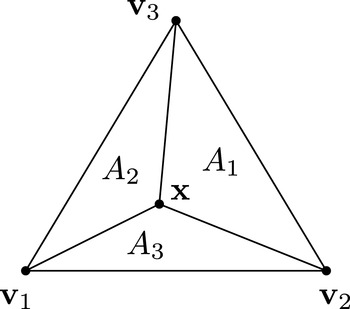
partitions it into the three sub-triangles indicated in Figure 1.1, and the three barycentric coordinates of
 $\mathbf{x}$
are the ratios of the areas
 $A_{i}$
of the sub-triangles to the area
 $A$
of
 $T$
, that is,
 $$\begin{eqnarray}\mathbf{x}={\it\phi}_{1}\boldsymbol{v}_{1}+{\it\phi}_{2}\boldsymbol{v}_{2}+{\it\phi}_{3}\boldsymbol{v}_{3},\end{eqnarray}$$
where
 $$\begin{eqnarray}{\it\phi}_{i}=\frac{A_{i}}{A},\quad i=1,2,3.\end{eqnarray}$$
In a similar way, a point
 $\mathbf{x}$
in a tetrahedron
 $T\subset \mathbb{R}^{3}$
induces a partition of
 $T$
into four sub-tetrahedra, and the ratios of their volumes to the volume of
 $T$
define the four barycentric coordinates of
 $\mathbf{x}$
. This construction generalizes to any simplex in any space dimension.
Coordinates in a triangle.

An important application of such coordinates is their use in defining Bernstein–Bézier polynomials over simplices. For example, in the triangular case, the coordinates
 ${\it\phi}_{i}$
,
 $i=1,2,3$
, are linear functions of
 $\mathbf{x}$
, and the BB-polynomials of degree
 $d$
are
 $$\begin{eqnarray}B_{\mathbf{i},d}(\mathbf{x})=\frac{d!}{i_{1}!i_{2}!i_{3}!}{\it\phi}_{1}^{i_{1}}(\mathbf{x}){\it\phi}_{2}^{i_{2}}(\mathbf{x}){\it\phi}_{3}^{i_{3}}(\mathbf{x}),\quad |\mathbf{i}|=d,\end{eqnarray}$$
where
 $\mathbf{i}=(i_{1},i_{2},i_{3})\in \mathbb{N}_{0}^{3}$
, and
 $|\mathbf{i}|=i_{1}+i_{2}+i_{3}$
. These
 $\binom{d+2}{2}$
polynomials form a basis for the linear space of bivariate polynomials of (total) degree
 $\leq d$
and play a prominent role in numerical analysis, including the modelling of surfaces, both surface design and surface approximation, and in finite element methods (Prautzsch, Boehm and Paluszny Reference Prautzsch, Boehm and Paluszny2002, Lai and Schumaker Reference Lai and Schumaker2007, Farouki Reference Farouki2012).
In recent years there has been growing interest in the construction and application of various generalizations of barycentric coordinates to polygons and polyhedra, which includes both curve and surface modelling, and finite element methods. The purpose of this paper is to review these constructions, their properties, and applications.
2. Barycentric coordinates on convex polygons
Vertex ordering for a polygon.

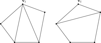
Partitions for
 $L_{i}$
and
 $\ell _{i}$
.

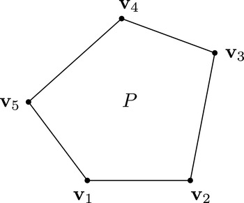
Let
 $P\subset \mathbb{R}^{2}$
be a convex polygon, viewed as an open set, with vertices
 $\boldsymbol{v}_{1},\boldsymbol{v}_{2},\ldots ,\boldsymbol{v}_{n}$
,
 $n\geq 3$
, in some anticlockwise ordering. Figure 2.1 shows an example with
 $n=5$
. Any functions
 ${\it\phi}_{i}\,:\,P\rightarrow \mathbb{R}$
,
 $i=1,\ldots ,n$
, will be called generalized barycentric coordinates (GBCs) if, for all
 $\mathbf{x}\in P$
,
 ${\it\phi}_{i}(\mathbf{x})\geq 0$
,
 $i=1,\ldots ,n$
, and
 $$\begin{eqnarray}\mathop{\sum }_{i=1}^{n}{\it\phi}_{i}(\mathbf{x})=1,\quad \mathop{\sum }_{i=1}^{n}{\it\phi}_{i}(\mathbf{x})\boldsymbol{v}_{i}=\mathbf{x}.\end{eqnarray}$$
For
 $n\!=\!3$
, the functions
 ${\it\phi}_{1},{\it\phi}_{2},{\it\phi}_{3}$
are uniquely determined from (2.1) and are the usual triangular barycentric coordinates with respect to the triangle
 $P$
,
 $$\begin{eqnarray}{\it\phi}_{i}(\mathbf{x})=\frac{A(\mathbf{x},\boldsymbol{v}_{i+1},\boldsymbol{v}_{i+2})}{A(\boldsymbol{v}_{1},\boldsymbol{v}_{2},\boldsymbol{v}_{3})},\quad i=1,2,3,\end{eqnarray}$$
and
 $A(\mathbf{x}_{1},\mathbf{x}_{2},\mathbf{x}_{3})$
is the signed area of the triangle with vertices
 $\mathbf{x}_{k}=(x_{k},y_{k})$
,
 $k=1,2,3$
:
 $$\begin{eqnarray}A(\mathbf{x}_{1},\mathbf{x}_{2},\mathbf{x}_{3}):=\frac{1}{2}\left|\begin{array}{@{}ccc@{}}1 & 1 & 1\\ x_{1} & x_{2} & x_{3}\\ y_{1} & y_{2} & y_{3}\end{array}\right|\!.\end{eqnarray}$$
Here and throughout, vertices are indexed cyclically, i.e.,
 $\boldsymbol{v}_{n+1}:=\boldsymbol{v}_{1}$
, etc.
For
 $n\geq 4$
, the choice of
 ${\it\phi}_{1},\ldots ,{\it\phi}_{n}$
is no longer unique. However, they share some basic properties, derived in Floater, Hormann and Kós (Reference Floater, Hormann and Kós2006).
-
∙ The functions
 ${\it\phi}_{i}$
have a unique continuous extension to
$\partial P$
, the boundary of
$P$
.
-
∙ Lagrange property:
${\it\phi}_{i}(\boldsymbol{v}_{j})={\it\delta}_{ij}$
. -
∙ Piecewise linearity on
$\partial P$
: (2.2)
$$\begin{eqnarray}{\it\phi}_{i}((1-{\it\mu})\boldsymbol{v}_{j}+{\it\mu}\boldsymbol{v}_{j+1})=(1-{\it\mu}){\it\phi}_{i}(\boldsymbol{v}_{j})+{\it\mu}{\it\phi}_{i}(\boldsymbol{v}_{j+1}),\quad {\it\mu}\in [0,1].\end{eqnarray}$$
-
∙ Interpolation: if
(2.3)then
$$\begin{eqnarray}g(\mathbf{x})=\mathop{\sum }_{i=1}^{n}{\it\phi}_{i}(\mathbf{x})f(\boldsymbol{v}_{i}),\quad \mathbf{x}\in P,\end{eqnarray}$$
$g(\boldsymbol{v}_{i})=f(\boldsymbol{v}_{i})$
. We call
$g$
a barycentric interpolant to
$f$
.
-
∙ Linear precision: if
$f$
is linear then
$g=f$
. -
∙
$\ell _{i}\leq {\it\phi}_{i}\leq L_{i}$
where
$L_{i},\ell _{i}\,:\,P\rightarrow \mathbb{R}$
are the continuous, piecewise linear functions over the partitions of
$P$
shown in Figure 2.2 satisfying
$L_{i}(\boldsymbol{v}_{j})=\ell _{i}(\boldsymbol{v}_{j})={\it\delta}_{ij}$
.
$L_{i}$
is the least upper bound on
${\it\phi}_{i}$
and
$\ell _{i}$
the greatest lower bound.





3. Inverse bilinear coordinates
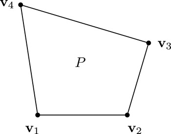
The first GBCs we study are specialized to quadrilaterals. Thus, suppose
 $n=4$
, as in Figure 3.1. GBCs can be constructed in this case by viewing
 $P$
as the image of a bilinear map from the unit square
 $[0,1]\times [0,1]$
. Such maps are commonly used in computer graphics (Wolberg Reference Wolberg1990) and finite element methods. For each
 $\mathbf{x}\in P$
, there exist unique
 ${\it\lambda},{\it\mu}\in (0,1)$
such that
 $$\begin{eqnarray}(1-{\it\lambda})(1-{\it\mu})\boldsymbol{v}_{1}+{\it\lambda}(1-{\it\mu})\boldsymbol{v}_{2}+{\it\lambda}{\it\mu}\boldsymbol{v}_{3}+(1-{\it\lambda}){\it\mu}\boldsymbol{v}_{4}=\mathbf{x},\end{eqnarray}$$
and so the four functions
 $$\begin{eqnarray}{\it\phi}_{1}(\mathbf{x})=(1-{\it\lambda})(1-{\it\mu}),\quad {\it\phi}_{2}(\mathbf{x})={\it\lambda}(1-{\it\mu}),\quad {\it\phi}_{3}(\mathbf{x})={\it\lambda}{\it\mu},\quad {\it\phi}_{4}(\mathbf{x})=(1-{\it\lambda}){\it\mu}\end{eqnarray}$$
are barycentric coordinates for
 $\mathbf{x}$
, that is, they are positive and satisfy (2.1). To find
 ${\it\phi}_{i}$
,
 $i=1,2,3,4$
, as functions of the point
 $\mathbf{x}$
, it remains to find
 ${\it\lambda}$
and
 ${\it\mu}$
as functions of
 $\mathbf{x}$
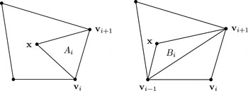
, that is, to find the inverse of the bilinear map. To do this, define the triangle areas
 $$\begin{eqnarray}A_{i}(\mathbf{x})=A(\mathbf{x},\boldsymbol{v}_{i},\boldsymbol{v}_{i+1}),\quad i=1,2,3,4,\end{eqnarray}$$
and
 $$\begin{eqnarray}B_{i}(\mathbf{x})=A(\mathbf{x},\boldsymbol{v}_{i-1},\boldsymbol{v}_{i+1}),\quad i=1,2,3,4;\end{eqnarray}$$
see Figure 3.2. We will also use these definitions later for other polygons, but note that in this quadrilateral case,
 $B_{3}=-B_{1}$
and
 $B_{4}=-B_{2}$
.
Convex quadrilateral.

Area
 $A_{i}$
and signed area
 $B_{i}$
.

We now show the following.
Theorem 3.1.
 $$\begin{eqnarray}({\it\mu},1-{\it\lambda},1-{\it\mu},{\it\lambda})=(2A_{i}/E_{i})_{i=1,2,3,4},\end{eqnarray}$$
where
 $$\begin{eqnarray}E_{i}=2A_{i}-B_{i}-B_{i+1}+\sqrt{D},\quad i=1,2,3,4,\end{eqnarray}$$
and
 $$\begin{eqnarray}D=B_{1}^{2}+B_{2}^{2}+2A_{1}A_{3}+2A_{2}A_{4}.\end{eqnarray}$$
Therefore,
 $$\begin{eqnarray}{\it\phi}_{i}=\frac{4A_{i+1}A_{i+2}}{E_{i+1}E_{i+2}},\quad i=1,2,3,4.\end{eqnarray}$$
Proof. It is sufficient to show that
 $$\begin{eqnarray}{\it\mu}=\frac{2A_{1}}{E_{1}}=\frac{2A_{1}}{2A_{1}-B_{1}-B_{2}+\sqrt{D}}\end{eqnarray}$$
as the derivation of the other three terms in (3.2) is similar. Defining the four vectors
 $\mathbf{d}_{i}=\boldsymbol{v}_{i}-\mathbf{x}$
,
 $i=1,2,3,4$
, (3.1) can be expressed as
 $$\begin{eqnarray}(1-{\it\lambda})(1-{\it\mu})\mathbf{d}_{1}+{\it\lambda}(1-{\it\mu})\mathbf{d}_{2}+{\it\lambda}{\it\mu}\mathbf{d}_{3}+(1-{\it\lambda}){\it\mu}\mathbf{d}_{4}=0.\end{eqnarray}$$
Next, divide the equation by
 ${\it\lambda}{\it\mu}$
, and defining
 $$\begin{eqnarray}{\it\alpha}:=\frac{1-{\it\lambda}}{{\it\lambda}},\quad {\it\beta}:=\frac{1-{\it\mu}}{{\it\mu}},\end{eqnarray}$$
the equation becomes
 $$\begin{eqnarray}{\it\alpha}{\it\beta}\mathbf{d}_{1}+{\it\beta}\mathbf{d}_{2}+\mathbf{d}_{3}+{\it\alpha}\mathbf{d}_{4}=0.\end{eqnarray}$$
By writing this as
 $$\begin{eqnarray}{\it\alpha}({\it\beta}\mathbf{d}_{1}+\mathbf{d}_{4})+({\it\beta}\mathbf{d}_{2}+\mathbf{d}_{3})=0,\end{eqnarray}$$
and taking the cross product of it with
 ${\it\beta}\mathbf{d}_{1}+\mathbf{d}_{4}$
eliminates
 ${\it\alpha}$
:
 $$\begin{eqnarray}({\it\beta}\mathbf{d}_{1}+\mathbf{d}_{4})\times ({\it\beta}\mathbf{d}_{2}+\mathbf{d}_{3})=0.\end{eqnarray}$$
(Here,
 $\mathbf{a}\times \mathbf{b}=(a_{1},a_{2})\times (b_{1},b_{2}):=a_{1}b_{2}-a_{2}b_{1}$
.) This is a quadratic equation in
 ${\it\beta}$
, which, in terms of the
 $A_{i}$
and
 $B_{i}$
, is
 $$\begin{eqnarray}A_{1}{\it\beta}^{2}+(B_{1}+B_{2}){\it\beta}-A_{3}=0.\end{eqnarray}$$
The discriminant is
 $$\begin{eqnarray}D=(B_{1}+B_{2})^{2}+4A_{1}A_{3}>0,\end{eqnarray}$$
and so the equation has real roots, and
 ${\it\beta}$
is the positive one,
 $$\begin{eqnarray}{\it\beta}=\frac{-B_{1}-B_{2}+\sqrt{D}}{2A_{1}}.\end{eqnarray}$$
Next observe that
 $$\begin{eqnarray}B_{1}B_{2}=A_{2}A_{4}-A_{1}A_{3},\end{eqnarray}$$
which follows from taking the cross product of
 $\mathbf{d}_{4}$
with the well-known equation
 $$\begin{eqnarray}(\mathbf{d}_{1}\times \mathbf{d}_{2})\mathbf{d}_{3}+(\mathbf{d}_{2}\times \mathbf{d}_{3})\mathbf{d}_{1}+(\mathbf{d}_{3}\times \mathbf{d}_{1})\mathbf{d}_{2}=0.\end{eqnarray}$$
From this we find that
 $D$
can be expressed as (3.3). From
 ${\it\beta}$
we now obtain
 ${\it\mu}=1/(1+{\it\beta})$
.☐
4. Wachspress coordinates
Wachspress coordinates have the advantage over inverse bilinear coordinates that they apply to any convex polygon, and moreover, they are rational functions, having no square roots. These coordinates and their generalizations due to Warren and others (Wachspress Reference Wachspress1975, Warren Reference Warren1996, Meyer, Barr, Lee and Desbrun Reference Meyer, Barr, Lee and Desbrun2002, Warren, Schaefer, Hirani and Desbrun Reference Warren, Schaefer, Hirani and Desbrun2007, Ju, Schaefer, Warren and Desbrun Reference Ju, Schaefer, Warren and Desbrun2005b , Wachspress Reference Wachspress2011) are therefore an attractive choice. Their derivatives are relatively easy to evaluate, and some simple upper bounds on their gradients have been found recently (Floater, Gillette and Sukumar Reference Floater, Gillette and Sukumar2014), justifying their use as shape functions for polygonal finite elements.
Wachspress (Reference Wachspress1975) realized that for a convex
 $n$
-gon
 $P$
with
 $n\geq 4$
, there is no hope of finding barycentric coordinates that are polynomial. He showed, however, that one can succeed with rational functions. This requires choosing rational functions that reduce to linear univariate polynomials along the edges of
 $P$
. To achieve this, Wachspress used the following observation. Suppose
 $r(\mathbf{x})=r(x,y)$
is a bivariate rational function of degree
 $(m_{1},m_{2})$
, that is,
 $$\begin{eqnarray}r(x,y)=\frac{p(x,y)}{q(x,y)},\end{eqnarray}$$
where
 $p$
and
 $q$
are polynomials of total degree
 $m_{1}$
and
 $m_{2}$
respectively. If
 $L$
is any straight line given by the equation
 $$\begin{eqnarray}y=y(x)=c_{0}+c_{1}x,\end{eqnarray}$$
then along
 $L$
, the function
 $r$
is also rational,
 $$\begin{eqnarray}\tilde{r}(x):=r(x,y(x))=\frac{p(x,y(x))}{q(x,y(x))},\end{eqnarray}$$
and, in general,
 $\tilde{r}$
also has degree
 $(m_{1},m_{2})$
. However, if the two algebraic curves
 $p(x,y)=0$
and
 $q(x,y)=0$
intersect at some point
 $\mathbf{x}_{\ast }=(x_{\ast },y_{\ast })$
and
 $L$
also passes through
 $\mathbf{x}_{\ast }$
, so that
 $y_{\ast }=c_{0}+c_{1}x_{\ast }$
, then both
 $p(x,y(x))$
and
 $q(x,y(x))$
contain a factor of
 $(x-x_{\ast })$
. These factors cancel and
 $\tilde{r}$
has degree at most
 $(m_{1}-1,m_{2}-1)$
. This same ‘cancellation principle’ applies when
 $L$
passes through
 $k$
intersections of the curves
 $p(x,y)=0$
and
 $q(x,y)=0$
. The degree of
 $\tilde{r}$
is then at most
 $(m_{1}-k,m_{2}-k)$
.
This idea led Wachspress (Reference Wachspress1975, Sections 5.1, 5.2) to define
 $$\begin{eqnarray}{\it\phi}_{i}(\mathbf{x})=\frac{k_{i}p^{i}(\mathbf{x})}{q_{n-3}(\mathbf{x})},\quad i=1,\ldots ,n.\end{eqnarray}$$
Here
 $p^{i}$
is the polynomial of degree
 $n-2$
,
 $$\begin{eqnarray}p^{i}(\mathbf{x})=\mathop{\prod }_{j\neq i-1,i}l_{j}(\mathbf{x}),\end{eqnarray}$$
with
 $l_{j}$
any non-trivial linear polynomial that is zero on the line through the edge
 $\mathbf{e}_{j}:=[\boldsymbol{v}_{j},\boldsymbol{v}_{j+1}]$
;
 $q_{n-3}$
is the ‘adjoint’ polynomial of the polygon, that is, the unique polynomial of degree
 $\leq n-3$
that vanishes at all the ‘exterior intersection points’ of the polygon
 $P$
, that is, all intersection points between lines extending through the edges of
 $P$
(which for some polygons may be points at infinity);
 $k_{i}$
is the ‘normalizing factor’
 $$\begin{eqnarray}k_{i}=\frac{q_{n-3}(\boldsymbol{v}_{i})}{p^{i}(\boldsymbol{v}_{i})},\end{eqnarray}$$
which ensures that
 ${\it\phi}_{i}(\boldsymbol{v}_{i})=1$
.
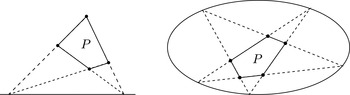
Figure 4.1 shows the adjoint curve,
 $q_{n-3}=0$
, for a quadrilateral and a pentagon: the first a straight line, the second an ellipse.
Adjoint curves.

By definition,
 ${\it\phi}_{i}$
is zero on all edges of
 $P$
that are not adjacent to
 $\boldsymbol{v}_{i}$
, that is, on
 $\mathbf{e}_{j}$
,
 $j\neq i-1,i$
. By the cancellation principle,
 ${\it\phi}_{i}$
is linear along the two edges that are adjacent to
 $\boldsymbol{v}_{i}$
, that is, along
 $\mathbf{e}_{i-1}$
and
 $\mathbf{e}_{i}$
, because the extensions of these two edges pass through
 $n-3$
intersection points of the adjoint curve
 $q_{n-3}=0$
with
 $n-3$
of the other extended edges of
 $P$
: for
 $\mathbf{e}_{i}$
these edges are
 $\mathbf{e}_{j}$
,
 $j\neq i-1,i,i+1$
, and for
 $\mathbf{e}_{i-1}$
they are
 $\mathbf{e}_{j}$
,
 $j\neq i-2,i-1,i$
. Since
 ${\it\phi}_{i}(\boldsymbol{v}_{i})=1$
, this establishes that
 ${\it\phi}_{i}$
has the piecewise linear property (2.2) on
 $\partial P$
. This means that the barycentric property (2.1) holds for
 $\mathbf{x}\in \partial P$
, and since the
 ${\it\phi}_{i}$
have a common denominator of
 $q_{n-3}$
, it follows that the barycentric property extends to all
 $\mathbf{x}\in P$
.
The degrees,
 $n-2$
and
 $n-3$
, of the numerator and denominator of
 ${\it\phi}_{i}$
agree with the triangular case where
 $n=3$
and the coordinates are linear functions.
Wachspress applied the same ideas to construct coordinates for so-called ‘polycons’, planar regions whose sides are either straight lines or conics, with some restrictions. The coordinates are again linear along the edges, straight or conic, but are not in general positive when some of the edges are conic. A method for constructing the adjoint in the general case was proposed by Dasgupta and Wachspress (Reference Dasgupta and Wachspress2008).
Warren (Reference Warren1996) gave an alternative derivation of the coordinates for polygons (and polytopes), defining the adjoint polynomial in a different way.
4.1. Triangle areas
Meyer et al. (Reference Meyer, Barr, Lee and Desbrun2002) found a simpler way of defining Wachspress’s coordinates, avoiding the adjoint, using instead the triangle areas
 $$\begin{eqnarray}A_{i}=A_{i}(\mathbf{x})=A(\mathbf{x},\boldsymbol{v}_{i},\boldsymbol{v}_{i+1}),\quad C_{i}=A(\boldsymbol{v}_{i-1},\boldsymbol{v}_{i},\boldsymbol{v}_{i+1}),\end{eqnarray}$$
and the formula
 $$\begin{eqnarray}{\it\phi}_{i}(\mathbf{x})=\frac{w_{i}(\mathbf{x})}{\mathop{\sum }_{j=1}^{n}w_{j}(\mathbf{x})},\end{eqnarray}$$
where
 $$\begin{eqnarray}w_{i}(\mathbf{x})=\frac{C_{i}}{A_{i-1}(\mathbf{x})A_{i}(\mathbf{x})};\end{eqnarray}$$
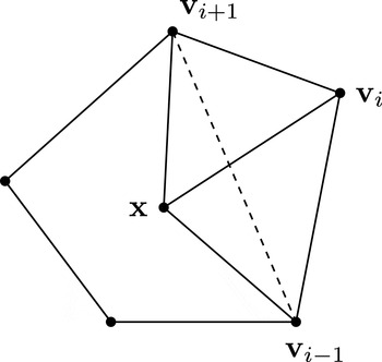
see Figure 4.2.
Areas defining the weight function
 $w_{i}$
.

Meyer et al. (Reference Meyer, Barr, Lee and Desbrun2002) showed independently that the coordinates (4.2) are barycentric as follows. Due to (4.2), it is sufficient to show that
 $$\begin{eqnarray}\mathop{\sum }_{i=1}^{n}w_{i}(\mathbf{x})(\boldsymbol{v}_{i}-\mathbf{x})=0.\end{eqnarray}$$
We can express any
 $\mathbf{x}\in P$
as a barycentric combination of
 $\boldsymbol{v}_{i-1},\boldsymbol{v}_{i},\boldsymbol{v}_{i+1}$
,
 $$\begin{eqnarray}\mathbf{x}=\frac{A_{i}}{C_{i}}\boldsymbol{v}_{i-1}+\frac{(C_{i}-A_{i-1}-A_{i})}{C_{i}}\boldsymbol{v}_{i}+\frac{A_{i-1}}{C_{i}}\boldsymbol{v}_{i+1},\end{eqnarray}$$
whether or not
 $\mathbf{x}$
lies inside the triangle formed by
 $\boldsymbol{v}_{i-1},\boldsymbol{v}_{i},\boldsymbol{v}_{i+1}$
. This equation can be rearranged in the form
 $$\begin{eqnarray}\frac{C_{i}}{A_{i-1}A_{i}}(\boldsymbol{v}_{i}-\mathbf{x})=\frac{1}{A_{i-1}}(\boldsymbol{v}_{i}-\boldsymbol{v}_{i-1})-\frac{1}{A_{i}}(\boldsymbol{v}_{i+1}-\boldsymbol{v}_{i}).\end{eqnarray}$$
Summing both sides of this over
 $i$
, and observing that the right-hand side then cancels to zero, gives
 $$\begin{eqnarray}\mathop{\sum }_{i=1}^{n}\frac{C_{i}}{A_{i-1}A_{i}}(\boldsymbol{v}_{i}-\mathbf{x})=0,\end{eqnarray}$$
which proves (4.3).
Note that if the polygon
 $P$
is regular, the area
 $C_{i}$
is the same for all
 $i$
, in which case
 $w_{i}$
in (4.2) can be reduced to
 $$\begin{eqnarray}w_{i}(\mathbf{x})=\frac{1}{A_{i-1}(\mathbf{x})A_{i}(\mathbf{x})}.\end{eqnarray}$$
Loop and DeRose (Reference Loop and DeRose1989) suggested these simpler weight functions for any regular
 $n$
-gon, and gave a different proof that the coordinates
 ${\it\phi}_{i}$
in this case are barycentric.
Multiplying the numerator and denominator of (4.2) by the product of all the
 $A_{j}$
gives the alternative form
 $$\begin{eqnarray}{\it\phi}_{i}(\mathbf{x})=\frac{{\hat{w}}_{i}(\mathbf{x})}{\mathop{\sum }_{j=1}^{n}{\hat{w}}_{j}(\mathbf{x})},\quad {\hat{w}}_{i}(\mathbf{x})=C_{i}\mathop{\prod }_{j\neq i-1,i}A_{j}(\mathbf{x}),\end{eqnarray}$$
and since each area
 $A_{j}(\mathbf{x})$
is linear in
 $\mathbf{x}$
, we see from this that
 ${\it\phi}_{i}$
is a rational function, with degree
 $\leq n-2$
in the numerator and denominator. In fact, the denominator has degree
 $\leq n-3$
due to the linear precision of the
 ${\it\phi}_{i}$
.
It follows from (4.7) that if we normalize the
 $l_{j}$
defining
 $p^{i}$
in (4.1) by setting
 $l_{j}(\mathbf{x})=A_{j}(\mathbf{x})$
, then we can take
 $k_{i}=C_{i}$
and
 $$\begin{eqnarray}q_{n-3}(\mathbf{x})=\mathop{\sum }_{i=1}^{n}C_{i}p^{i}(\mathbf{x}).\end{eqnarray}$$
We note that the ‘global’ form of
 ${\it\phi}_{i}(\mathbf{x})$
in (4.7) is also valid for
 $\mathbf{x}\in \partial P$
, unlike the ‘local’ form (4.2), though it requires more computation for large
 $n$
.
4.2. Perpendicular distances to edges
An alternative way of expressing Wachspress coordinates is in terms of the perpendicular distances of
 $\mathbf{x}$
to the edges of
 $P$
. This is the form used by Warren et al. (Reference Warren, Schaefer, Hirani and Desbrun2007), and it generalizes in a natural way to higher dimension.
For each
 $i$
, let
 $\mathbf{n}_{i}\in \mathbb{R}^{2}$
be the outward unit normal to the edge
 $e_{i}=[\boldsymbol{v}_{i},\boldsymbol{v}_{i+1}]$
, and for any
 $\mathbf{x}\in P$
let
 $h_{i}(\mathbf{x})$
be the perpendicular distance of
 $\mathbf{x}$
to the edge
 $e_{i}$
, so that
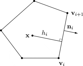
 $$\begin{eqnarray}h_{i}(\mathbf{x})=(\boldsymbol{v}_{i}-\mathbf{x})\cdot \mathbf{n}_{i}=(\boldsymbol{v}_{i+1}-\mathbf{x})\cdot \mathbf{n}_{i};\end{eqnarray}$$
see Figure 4.3. Then the coordinates in (4.2) can be expressed as
 $$\begin{eqnarray}{\it\phi}_{i}(\mathbf{x})=\frac{\tilde{w}_{i}(\mathbf{x})}{\mathop{\sum }_{j=1}^{n}\tilde{w}_{j}(\mathbf{x})},\end{eqnarray}$$
where
 $$\begin{eqnarray}\tilde{w}_{i}(\mathbf{x}):=\frac{\mathbf{n}_{i-1}\times \mathbf{n}_{i}}{h_{i-1}(\mathbf{x})h_{i}(\mathbf{x})},\end{eqnarray}$$
and
 $$\begin{eqnarray}\mathbf{x}_{1}\times \mathbf{x}_{2}:=|\begin{array}{@{}cc@{}}x_{1} & x_{2}\\ y_{1} & y_{2}\end{array}| ,\end{eqnarray}$$
for
 $\mathbf{x}_{k}=(x_{k},y_{k})$
. To see this, observe that with
 $L_{j}=\Vert \boldsymbol{v}_{j+1}-\boldsymbol{v}_{j}\Vert$
, and
 $\Vert \cdot \Vert$
the Euclidean norm, and
 ${\it\beta}_{i}$
the interior angle of the polygon at
 $\boldsymbol{v}_{i}$
,
 $$\begin{eqnarray}C_{i}=\frac{1}{2}\sin {\it\beta}_{i}L_{i-1}L_{i},\quad A_{i-1}=\frac{1}{2}h_{i-1}L_{i-1},\quad A_{i}=\frac{1}{2}h_{i}L_{i},\end{eqnarray}$$
so that
 $$\begin{eqnarray}w_{i}(\mathbf{x})=2\tilde{w}_{i}(\mathbf{x}).\end{eqnarray}$$
If the polygon
 $P$
is regular, the weight function
 $\tilde{w}_{i}$
in (4.8) can be replaced by
 $$\begin{eqnarray}\tilde{w}_{i}(\mathbf{x})=\frac{1}{h_{i-1}(\mathbf{x})h_{i}(\mathbf{x})},\end{eqnarray}$$
in analogy to (4.6). For a regular pentagon these were the weight functions proposed by Charrot and Gregory (Reference Charrot and Gregory1984) for constructing five-sided surface patches.
Perpendicular distances.

4.3. Gradients
The gradient of a Wachspress coordinate can be found quite easily from the perpendicular form (4.8)–(4.9). Since
 ${\rm\nabla}h_{i}(\mathbf{x})=-\mathbf{n}_{i}$
, the gradient of
 $\tilde{w}_{i}$
is (Floater et al.
Reference Floater, Gillette and Sukumar2014)
 $$\begin{eqnarray}{\rm\nabla}\tilde{w}_{i}(\mathbf{x})=\tilde{w}_{i}(\mathbf{x})\biggl(\frac{\mathbf{n}_{i-1}}{h_{i-1}(\mathbf{x})}+\frac{\mathbf{n}_{i}}{h_{i}(\mathbf{x})}\biggr).\end{eqnarray}$$
Thus the (vector-valued) ratio
 $$\begin{eqnarray}\mathbf{R}_{i}:={\rm\nabla}\tilde{w}_{i}/\tilde{w}_{i}\end{eqnarray}$$
is simply
 $$\begin{eqnarray}\mathbf{R}_{i}(\mathbf{x})=\frac{\mathbf{n}_{i-1}}{h_{i-1}(\mathbf{x})}+\frac{\mathbf{n}_{i}}{h_{i}(\mathbf{x})}.\end{eqnarray}$$
Using the formula (Floater et al. Reference Floater, Gillette and Sukumar2014)
 $$\begin{eqnarray}{\rm\nabla}{\it\phi}_{i}={\it\phi}_{i}\biggl(\mathbf{R}_{i}-\mathop{\sum }_{j=1}^{n}{\it\phi}_{j}\mathbf{R}_{j}\biggr)\end{eqnarray}$$
for any function
 ${\it\phi}_{i}$
of the form (4.8), we thus obtain
 ${\rm\nabla}{\it\phi}_{i}(\mathbf{x})$
for
 $\mathbf{x}\in P$
.
Wachspress mapping.

4.4. Barycentric mapping
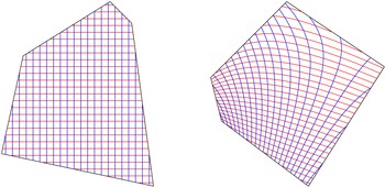
While Wachspress’s motivation for these coordinates was finite element methods, Warren suggested their use in deforming curves. The coordinates can be used to define a barycentric mapping of one polygon to another, and such a mapping will then map, or deform, a curve embedded in the first polygon into a new one, with the vertices of the polygon acting as control points, with an effect similar to those of Bézier and spline curves and surfaces.
Assuming the second polygon is
 $\tilde{P}$
with vertices
 $\tilde{\boldsymbol{v}}_{1},\ldots ,\tilde{\boldsymbol{v}}_{n}$
, the barycentric mapping
 $\mathbf{g}\,:\,P\rightarrow \tilde{P}$
is defined as follows. Given
 $\mathbf{x}\in P$
,
-
(1) express
$\mathbf{x}$
in Wachspress coordinates,
$\mathbf{x}=\sum _{i=1}^{n}{\it\phi}_{i}(\mathbf{x})\boldsymbol{v}_{i}$
, -
(2) set
$\mathbf{g}(\mathbf{x})=\sum _{i=1}^{n}{\it\phi}_{i}(\mathbf{x})\tilde{\boldsymbol{v}}_{i}$
.



Figure 4.4 shows such a mapping.
It is now known that Wachspress mappings between convex polygons are always injective, as shown in Floater and Kosinka (Reference Floater and Kosinka2010b
). The basic idea of the proof is to show that
 $\mathbf{g}$
has a positive Jacobian determinant
 $J(\mathbf{g})$
. To do this, one first shows that
 $J(\mathbf{g})$
can be expressed as
 $$\begin{eqnarray}J(\mathbf{g})=2\mathop{\sum }_{1\leq i<j<k\leq n}\left|\begin{array}{@{}ccc@{}}{\it\phi}_{i} & {\it\phi}_{j} & {\it\phi}_{k}\\ \partial _{1}{\it\phi}_{i} & \partial _{1}{\it\phi}_{j} & \partial _{1}{\it\phi}_{k}\\ \partial _{2}{\it\phi}_{i} & \partial _{2}{\it\phi}_{j} & \partial _{2}{\it\phi}_{k}\end{array}\right|A(\tilde{\boldsymbol{v}}_{i},\tilde{\boldsymbol{v}}_{j},\tilde{\boldsymbol{v}}_{k}).\end{eqnarray}$$
By the convexity of
 $\tilde{P}$
, the signed areas
 $A(\tilde{\boldsymbol{v}}_{i},\tilde{\boldsymbol{v}}_{j},\tilde{\boldsymbol{v}}_{k})$
in the sum are all positive, and so
 $J(\mathbf{g})>0$
if all the
 $3\times 3$
determinants in the sum are positive; this turns out to be the case for Wachspress coordinates
 ${\it\phi}_{i}$
.
4.5. Polygonal finite elements
There has been steadily growing interest in using generalized barycentric coordinates for finite element methods on polygonal and polyhedral meshes (Gillette, Rand and Bajaj Reference Gillette, Rand and Bajaj2012, Rand, Gillette and Bajaj Reference Rand, Gillette and Bajaj2013, Sukumar and Tabarraei Reference Sukumar and Tabarraei2004, Wicke, Botsch and Gross Reference Wicke, Botsch and Gross2007, Talischi, Paulino and Le Reference Talischi, Paulino and Le2009, Floater et al.
Reference Floater, Gillette and Sukumar2014, Manzini, Russo and Sukumar Reference Manzini, Russo and Sukumar2014, Bishop Reference Bishop2014). In order to establish the convergence of the finite element method, one needs to derive a bound on the gradients of the coordinates in terms of the geometry of the polygon
 $P$
. Upper bounds on
 $$\begin{eqnarray}\sup _{\mathbf{x}\in P}\Vert {\rm\nabla}{\it\phi}_{i}(\mathbf{x})\Vert\end{eqnarray}$$
were derived by Gillette et al. (Reference Gillette, Rand and Bajaj2012) for various types of coordinates, and by Rand et al. (Reference Rand, Gillette and Bajaj2013) for mean value coordinates. For Wachspress coordinates, a simpler bound was derived in Floater et al. (Reference Floater, Gillette and Sukumar2014). If we define, for
 $\mathbf{x}\in P$
,
 $$\begin{eqnarray}{\it\lambda}(\mathbf{x}):=\mathop{\sum }_{i=1}^{n}\Vert {\rm\nabla}{\it\phi}_{i}(\mathbf{x})\Vert ,\end{eqnarray}$$
then
 ${\it\lambda}$
plays a role similar to the Lebesgue function in the theory of polynomial interpolation, because for
 $g$
in (2.3),
 $$\begin{eqnarray}\Vert {\rm\nabla}g(\mathbf{x})\Vert \leq \mathop{\sum }_{i=1}^{n}\Vert {\rm\nabla}{\it\phi}_{i}(\mathbf{x})\Vert |f(\boldsymbol{v}_{i})|\leq {\it\lambda}(\mathbf{x})\max _{i=1,\ldots ,n}|f(\boldsymbol{v}_{i})|.\end{eqnarray}$$
Let
 $$\begin{eqnarray}{\rm\Lambda}:=\sup _{\mathbf{x}\in P}{\it\lambda}(\mathbf{x})\end{eqnarray}$$
be the corresponding ‘Lebesgue constant’. Recalling the perpendicular distances
 $h_{i}$
in the second formula for Wachspress coordinates (4.8)–(4.9), let
 $$\begin{eqnarray}h_{\ast }=\min _{i=1,\ldots ,n}\min _{j\neq i,i+1}h_{i}(\boldsymbol{v}_{j}),\end{eqnarray}$$
the minimum perpendicular distance between edges and vertices of the polygon. We will prove the following result.
Theorem 4.1. For Wachspress coordinates,
 $$\begin{eqnarray}{\rm\Lambda}\leq \frac{4}{h_{\ast }}.\end{eqnarray}$$
This is a special case of the theorem derived in Floater et al. (Reference Floater, Gillette and Sukumar2014) for simple convex polytopes in
 $\mathbb{R}^{d}$
.
Proof. Recalling the definition of
 $\mathbf{R}_{i}$
in (4.10), equation (4.11) shows that
 $$\begin{eqnarray}\mathbf{R}_{i}(\mathbf{x})=\mathbf{p}_{i-1}(\mathbf{x})+\mathbf{p}_{i}(\mathbf{x}),\end{eqnarray}$$
where
 $\mathbf{p}_{j}(\mathbf{x}):=\mathbf{n}_{j}/h_{j}(\mathbf{x})$
,
 $j=1,\ldots ,n$
. Substituting this into (4.12), and defining
 $$\begin{eqnarray}{\it\mu}_{j}:={\it\phi}_{j}+{\it\phi}_{j+1},\end{eqnarray}$$
gives
 $$\begin{eqnarray}\displaystyle \frac{{\rm\nabla}{\it\phi}_{i}}{{\it\phi}_{i}} & = & \displaystyle \mathbf{p}_{i-1}+\mathbf{p}_{i}-\mathop{\sum }_{j=1}^{n}{\it\phi}_{j}(\mathbf{p}_{j-1}+\mathbf{p}_{j})\nonumber\\ \displaystyle & = & \displaystyle \mathbf{p}_{i-1}+\mathbf{p}_{i}-\mathop{\sum }_{j=1}^{n}{\it\mu}_{j}\mathbf{p}_{j}\nonumber\\ \displaystyle & = & \displaystyle (1-{\it\mu}_{i-1})\mathbf{p}_{i-1}+(1-{\it\mu}_{i})\mathbf{p}_{i}-\mathop{\sum }_{j\neq i-1,i}{\it\mu}_{j}\mathbf{p}_{j},\nonumber\end{eqnarray}$$
and therefore, since
 $\Vert \mathbf{p}_{j}\Vert \leq 1/h_{j}$
,
 $$\begin{eqnarray}\Vert {\rm\nabla}{\it\phi}_{i}\Vert \leq A_{i}+B_{i},\end{eqnarray}$$
where
 $$\begin{eqnarray}A_{i}={\it\phi}_{i}\biggl(\frac{1-{\it\mu}_{i-1}}{h_{i-1}}+\frac{1-{\it\mu}_{i}}{h_{i}}\biggr),\quad B_{i}={\it\phi}_{i}\mathop{\sum }_{j\neq i-1,i}{\it\mu}_{j}\frac{1}{h_{j}}.\end{eqnarray}$$
Then,
 $$\begin{eqnarray}\mathop{\sum }_{i=1}^{n}A_{i}=\mathop{\sum }_{i=1}^{n}({\it\phi}_{i+1}+{\it\phi}_{i})\frac{1-{\it\mu}_{i}}{h_{i}}=C,\end{eqnarray}$$
where
 $$\begin{eqnarray}C=\mathop{\sum }_{i=1}^{n}{\it\mu}_{i}\frac{1-{\it\mu}_{i}}{h_{i}},\end{eqnarray}$$
and
 $$\begin{eqnarray}\mathop{\sum }_{i=1}^{n}B_{i}=\mathop{\sum }_{j=1}^{n}\mathop{\sum }_{i\neq j,j+1}{\it\phi}_{i}{\it\mu}_{j}\frac{1}{h_{j}}=\mathop{\sum }_{j=1}^{n}(1-{\it\mu}_{j}){\it\mu}_{j}\frac{1}{h_{j}}=C,\end{eqnarray}$$
as well. Thus,
 ${\it\lambda}$
in (4.13) is bounded as
 $$\begin{eqnarray}{\it\lambda}\leq 2C.\end{eqnarray}$$
In order to bound
 $C$
, we derive a bound on the ratio
 $(1-{\it\mu}_{i})/h_{i}$
. By the linear precision property of the coordinates
 ${\it\phi}_{i}$
,
 $$\begin{eqnarray}h_{i}(\mathbf{x})=\mathop{\sum }_{j=1}^{n}{\it\phi}_{j}(\mathbf{x})h_{i}(\boldsymbol{v}_{j})=\mathop{\sum }_{j\neq i,i+1}{\it\phi}_{j}(\mathbf{x})h_{i}(\boldsymbol{v}_{j})\geq \mathop{\sum }_{j\neq i,i+1}{\it\phi}_{j}(\mathbf{x})h_{\ast },\end{eqnarray}$$
and therefore
 $$\begin{eqnarray}\frac{1-{\it\mu}_{i}(\mathbf{x})}{h_{i}(\mathbf{x})}\leq \frac{1}{h_{\ast }}.\end{eqnarray}$$
Substituting this inequality into (4.14) implies
 $$\begin{eqnarray}C\leq \mathop{\sum }_{i=1}^{n}{\it\mu}_{i}\frac{1}{h_{\ast }}=2\mathop{\sum }_{i=1}^{n}{\it\phi}_{i}\frac{1}{h_{\ast }}=\frac{2}{h_{\ast }},\end{eqnarray}$$
which completes the proof.☐
It was further shown in Floater et al. (Reference Floater, Gillette and Sukumar2014) that the bound is sharp in the sense that the product
 $h_{\ast }{\rm\Lambda}$
can be arbitrarily close to
 $4$
. Specifically, it was shown that if
 $P$
is a regular
 $n$
-gon, then
 $$\begin{eqnarray}{\rm\Lambda}\geq \frac{2(1+\cos ({\it\pi}/n))}{h_{\ast }},\end{eqnarray}$$
in which case
 $$\begin{eqnarray}h_{\ast }{\rm\Lambda}\rightarrow 4,\quad \text{as }n\rightarrow \infty .\end{eqnarray}$$
5. Mean value coordinates
For star-shaped polygons, and arbitrary polygons, Wachspress coordinates are not well-defined, and mean value coordinates are perhaps the most popular kind of GBC. Even though they are no longer positive if the polygon is not star-shaped, they are very general and surprisingly robust over complex geometric shapes (Floater Reference Floater2003a , Floater, Kos and Reimers Reference Floater, Kos and Reimers2005, Ju, Schaefer and Warren Reference Ju, Schaefer and Warren2005a , Hormann and Floater Reference Hormann and Floater2006, Dyken and Floater Reference Dyken and Floater2009, Bruvoll and Floater Reference Bruvoll and Floater2010). They have been employed in various tasks in geometric modelling, such as surface parametrization, and plane and space deformation, as well as to shading and animation in computer graphics.
Suppose initially that the polygon
 $P$
is convex as before. Then the mean value (MV) coordinates are defined by (4.2) and
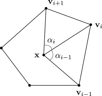
 $$\begin{eqnarray}w_{i}(\mathbf{x})=\frac{\tan ({\it\alpha}_{i-1}/2)+\tan ({\it\alpha}_{i}/2)}{\Vert \boldsymbol{v}_{i}-\mathbf{x}\Vert },\end{eqnarray}$$
with the angles
 ${\it\alpha}_{j}={\it\alpha}_{j}(\mathbf{x})$
, with
 $0<{\it\alpha}_{j}<{\it\pi}$
, as shown in Figure 5.1. To show that these coordinates are barycentric, it is sufficient, as in the Wachspress case, to show that the
 $w_{i}$
in (5.1) satisfy (4.3). This can be done in four steps.
-
(1) Express the unit vectors
$\mathbf{e}_{i}:=(\boldsymbol{v}_{i}-\mathbf{x})/\Vert \boldsymbol{v}_{i}-\mathbf{x}\Vert$
in polar coordinates, and note that
$$\begin{eqnarray}\mathbf{e}_{i}=(\cos {\it\theta}_{i},\sin {\it\theta}_{i}),\end{eqnarray}$$
${\it\alpha}_{i}={\it\theta}_{i+1}-{\it\theta}_{i}$
.
-
(2) Use the fact that the integral of the unit normals
$\mathbf{n}({\it\theta})=(\cos {\it\theta},\sin {\it\theta})$
on a circle is zero:
$$\begin{eqnarray}\int _{0}^{2{\it\pi}}\mathbf{n}({\it\theta})\text{d}{\it\theta}=0.\end{eqnarray}$$
-
(3) Split this integral according to the
${\it\theta}_{i}$
: (5.2)
$$\begin{eqnarray}\int _{0}^{2{\it\pi}}\mathbf{n}({\it\theta})\text{d}{\it\theta}=\mathop{\sum }_{i=1}^{n}\int _{{\it\theta}_{i}}^{{\it\theta}_{i+1}}\mathbf{n}({\it\theta})\,\text{d}{\it\theta}.\end{eqnarray}$$
-
(4) Show by trigonometry that
Substituting this into the sum in (5.2) and rearranging gives (4.3).
$$\begin{eqnarray}\int _{{\it\theta}_{i}}^{{\it\theta}_{i+1}}\mathbf{n}({\it\theta})\,\text{d}{\it\theta}=\frac{1-\cos {\it\alpha}_{i}}{\sin {\it\alpha}_{i}}(\mathbf{e}_{i}+\mathbf{e}_{i+1})=\tan ({\it\alpha}_{i}/2)(\mathbf{e}_{i}+\mathbf{e}_{i+1}).\end{eqnarray}$$






Notation for mean value coordinates.

We can compute the
 $w_{i}$
from
 $$\begin{eqnarray}\tan ({\it\alpha}_{i}/2)=(1-\cos {\it\alpha}_{i})/\sin {\it\alpha}_{i}\end{eqnarray}$$
and the scalar and cross products
 $$\begin{eqnarray}\cos {\it\alpha}_{i}=\mathbf{e}_{i}\cdot \mathbf{e}_{i+1},\quad \sin {\it\alpha}_{i}=\mathbf{e}_{i}\times \mathbf{e}_{i+1}.\end{eqnarray}$$
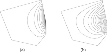
Figure 5.2 compares the contour lines of a Wachspress coordinate (a) with the corresponding MV coordinate (b).
5.1. Gradients
Similar to the Wachspress case, the gradient
 ${\rm\nabla}{\it\phi}_{i}$
of the MV coordinate
 ${\it\phi}_{i}$
can be computed from the formula (4.12) if we can find the ratio
 $\mathbf{R}_{i}:={\rm\nabla}w_{i}/w_{i}$
, with
 $w_{i}$
in (5.1). Let
 $r_{i}=\Vert \boldsymbol{v}_{i}-\mathbf{x}\Vert$
and
 $t_{i}=\tan ({\it\alpha}_{i}/2)$
so that
 $$\begin{eqnarray}w_{i}=\frac{t_{i-1}+t_{i}}{r_{i}}.\end{eqnarray}$$
Further, define
 $$\begin{eqnarray}\mathbf{c}_{i}=\frac{\mathbf{e}_{i}}{r_{i}}-\frac{\mathbf{e}_{i+1}}{r_{i+1}},\end{eqnarray}$$
and for a vector
 $\mathbf{a}=(a_{1},a_{2})\in \mathbb{R}^{2}$
, let
 $\mathbf{a}^{\bot }:=(-a_{2},a_{1})$
. It was shown in Floater (Reference Floater2014) that
 $$\begin{eqnarray}\mathbf{R}_{i}=\biggl(\frac{t_{i-1}}{t_{i-1}+t_{i}}\biggr)\frac{\mathbf{c}_{i-1}^{\bot }}{\sin {\it\alpha}_{i-1}}+\biggl(\frac{t_{i}}{t_{i-1}+t_{i}}\biggr)\frac{\mathbf{c}_{i}^{\bot }}{\sin {\it\alpha}_{i}}+\frac{\mathbf{e}_{i}}{r_{i}}.\end{eqnarray}$$
Other derivative formulas for MV coordinates can be found in Thiery, Tierny and Boubekeur (Reference Thiery, Tierny and Boubekeur2013).
(a) Wachspress. (b) Mean value.

5.2. Alternative formula
We saw that Wachspress coordinates can be expressed in the ‘global form’ (4.7), in which
 ${\it\phi}_{i}(\mathbf{x})$
is well-defined for
 $\mathbf{x}\in \partial P$
as well as for
 $\mathbf{x}\in P$
. It turns out that MV coordinates also have a global form with the same property, though for large
 $n$
the resulting expression requires more computation, and involves more square roots, than the local form based on (5.1). Let
 $\mathbf{d}_{i}=\boldsymbol{v}_{i}-\mathbf{x}$
,
 $i=1,\ldots ,n$
. It was shown in Floater (Reference Floater2014) that
 $$\begin{eqnarray}{\it\phi}_{i}(\mathbf{x})=\frac{{\hat{w}}_{i}(\mathbf{x})}{\mathop{\sum }_{j=1}^{n}{\hat{w}}_{j}(\mathbf{x})},\end{eqnarray}$$
where
 $$\begin{eqnarray}{\hat{w}}_{i}(\mathbf{x})=(r_{i-1}r_{i+1}-\mathbf{d}_{i-1}\cdot \mathbf{d}_{i+1})^{1/2}\mathop{\prod }_{j\neq i-1,i}(r_{j}r_{j+1}+\mathbf{d}_{j}\cdot \mathbf{d}_{j+1})^{1/2}.\end{eqnarray}$$
5.3. Star-shaped polygons
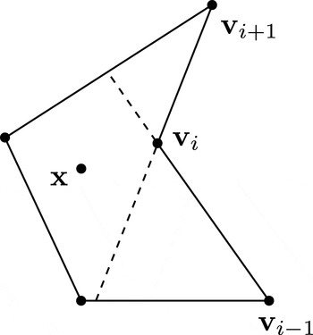
Mean value coordinates remain positive in the case that the polygon
 $P$
is star-shaped, and
 $\mathbf{x}$
belongs to its kernel, that is, if the line segment connecting
 $\mathbf{x}$
to
 $\boldsymbol{v}_{i}$
is inside
 $P$
for all
 $i=1,\ldots ,n$
; see Figure 5.3. In this case the angles
 ${\it\alpha}_{i}$
in (5.1) are again positive, and so
 $w_{i}$
and
 ${\it\phi}_{i}$
are also positive.
A star-shaped polygon and its kernel.

5.4. Mesh parametrization
The motivation for MV coordinates was for parametrizing triangular meshes (Tutte Reference Tutte1963, Floater Reference Floater1997, Floater Reference Floater2003b ), and subsequent surface fitting. When modelling geometry, triangular meshes are often used to represent surfaces, at least initially, one reason being that meshes are relatively easy to generate from point cloud data. However, we often want a smoother surface representation, and hence the need arises to fit a smooth parametric surface to the vertices of the mesh. This requires first making a suitable parametrization. Parametrizations are also useful for texture mapping and other processes in computer graphics.
We now describe a general method for constructing a parametrization of a triangular mesh in
 $\mathbb{R}^{3}$
that is homeomorphic to a disk. We denote by
 ${\mathcal{S}}$
the set of triangles in the mesh and
 $V$
its vertices and
 $E$
its edges. We let
 ${\rm\Omega}_{{\mathcal{S}}}\subset \mathbb{R}^{3}$
be the union of the triangles in
 ${\mathcal{S}}$
. Then we define a parametrization of
 ${\mathcal{S}}$
as a continuous piecewise linear mapping
 ${\it\psi}:{\rm\Omega}_{{\mathcal{S}}}\rightarrow \mathbb{R}^{2}$
. Then
 ${\it\psi}$
maps each vertex, edge, and triangle of
 ${\mathcal{S}}$
to a corresponding vertex, edge, and triangle in
 $\mathbb{R}^{2}$
. Such a mapping is completely determined by the points
 ${\it\psi}(\boldsymbol{v})$
,
 $\boldsymbol{v}\in V$
. Let
 $V_{I}$
denote the interior vertices of
 ${\mathcal{S}}$
and
 $V_{B}$
the boundary ones. The boundary vertices of
 ${\mathcal{S}}$
form a polygon
 $\partial {\mathcal{S}}$
in
 $\mathbb{R}^{3}$
which we call the boundary polygon of
 ${\mathcal{S}}$
. Two distinct vertices
 $\boldsymbol{v}$
and
 $\mathbf{w}$
in
 ${\mathcal{S}}$
are neighbours if they are the endpoints of some edge in
 ${\mathcal{S}}$
. For each
 $\boldsymbol{v}\in V$
, let
 $$\begin{eqnarray}N_{\boldsymbol{v}}=\{\mathbf{w}\in V:[\mathbf{w},\boldsymbol{v}]\in E\},\end{eqnarray}$$
the ‘1-ring neighbourhood’ of
 $\boldsymbol{v}$
.
The first step of the method is to choose any points
 ${\it\psi}(\boldsymbol{v})\in \mathbb{R}^{2}$
, for
 $\boldsymbol{v}\in V_{B}$
, such that the boundary polygon
 $\partial {\mathcal{S}}$
of
 ${\mathcal{S}}$
is mapped into a simple polygon
 ${\it\psi}(\partial {\mathcal{S}})$
in the plane (a polygon with no self-intersections). In the second step, for
 $\boldsymbol{v}\in V_{I}$
, we choose a set of strictly positive values
 ${\it\lambda}_{\boldsymbol{v}\mathbf{w}}$
, for
 $\mathbf{w}\in N_{\boldsymbol{v}}$
, such that
 $$\begin{eqnarray}\mathop{\sum }_{\mathbf{w}\in N_{\boldsymbol{v}}}{\it\lambda}_{\boldsymbol{v}\mathbf{w}}=1.\end{eqnarray}$$
Then we let the points
 ${\it\psi}(\boldsymbol{v})$
in
 $\mathbb{R}^{2}$
, for
 $\boldsymbol{v}\in V_{I}$
, be the unique solutions of the linear system of equations
 $$\begin{eqnarray}{\it\psi}(\boldsymbol{v})=\mathop{\sum }_{\mathbf{w}\in N_{\boldsymbol{v}}}{\it\lambda}_{\boldsymbol{v}\mathbf{w}}{\it\psi}(\mathbf{w}),\quad \boldsymbol{v}\in V_{I}.\end{eqnarray}$$
These equations force each interior point
 ${\it\psi}(\boldsymbol{v})$
to be a convex combination of its neighbouring points
 ${\it\psi}(\mathbf{w})$
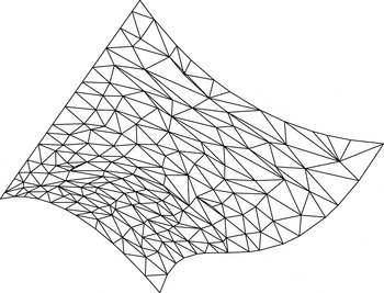
. Figure 5.4 shows an example of a triangular mesh
 ${\mathcal{S}}$
in
 $\mathbb{R}^{3}$
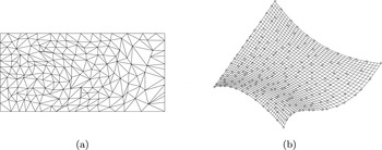
. Figure 5.5 shows a convex combination mapping of
 ${\mathcal{S}}$
, using MV weights, into a planar mesh
 ${\mathcal{T}}$
, whose boundary was chosen to be a rectangle. Figure 5.5 also shows a tensor-product bicubic spline approximation to the vertices of
 ${\mathcal{S}}$
based on their parameter points, the vertices of
 ${\mathcal{T}}$
. The spline surface was generated by least-squares approximation with a thin-plate spline smoothing term. Details can be found in Floater (Reference Floater2000).
Triangular mesh in
 $\mathbb{R}^{3}$
.

The linear system can be written in the form
 $$\begin{eqnarray}{\it\psi}(\boldsymbol{v})-\mathop{\sum }_{\mathbf{w}\in N_{\boldsymbol{v}}\cap V_{I}}{\it\lambda}_{\boldsymbol{v}\mathbf{w}}{\it\psi}(\mathbf{w})=\mathop{\sum }_{\mathbf{w}\in N_{\boldsymbol{v}}\cap V_{B}}{\it\lambda}_{\boldsymbol{v}\mathbf{w}}{\it\psi}(\mathbf{w}),\quad \boldsymbol{v}\in V_{I},\end{eqnarray}$$
or as the equation
 $$\begin{eqnarray}A\mathbf{x}=\mathbf{b},\end{eqnarray}$$
where
 $\mathbf{x}=({\it\psi}(\mathbf{w}))_{\mathbf{w}\in V_{I}}$
is the column vector of unknowns in some arbitrary ordering,
 $\mathbf{b}$
is the column vector whose elements are the right-hand sides of (5.6), and the square matrix
 $A=(a_{\boldsymbol{v}\mathbf{w}})_{\boldsymbol{v},\mathbf{w}\in V_{I}}$
has elements
 $$\begin{eqnarray}a_{\boldsymbol{v}\mathbf{w}}=\left\{\begin{array}{@{}ll@{}}1\quad & \mathbf{w}=\boldsymbol{v},\\ -{\it\lambda}_{\boldsymbol{v}\mathbf{w}}\quad & \mathbf{w}\in N_{\boldsymbol{v}},\\ 0\quad & \text{otherwise}.\end{array}\right.\end{eqnarray}$$
The existence and uniqueness of the solution to (5.5) follows from the structure of the matrix
 $A$
, namely that its off diagonal elements are either zero or negative and each row of
 $A$
is diagonally dominant. Moreover every row corresponding to a vertex
 $\boldsymbol{v}\in V_{I}$
which has at least one neighbour in
 $V_{B}$
is strictly diagonally dominant and every interior vertex can be connected to the boundary by a path of vertices. A standard result in linear algebra shows then that
 $A$
is non-singular. In fact
 $A$
is a so-called M-matrix. Such matrices arise naturally in various discretizations of differential operators.
This parametrization method is an extension of the method of Tutte (Reference Tutte1963) for drawing a planar graph. In Tutte’s method, the weights
 ${\it\lambda}_{\boldsymbol{v}\mathbf{w}}$
are ‘uniform’, that is, constant for each vertex
 $\boldsymbol{v}$
: specifically
 ${\it\lambda}_{\boldsymbol{v}\mathbf{w}}=1/d(\boldsymbol{v})$
,
 $\mathbf{w}\in N_{\boldsymbol{v}}$
, where
 $d(\boldsymbol{v})=\#(N_{\boldsymbol{v}})$
is the valency of
 $\boldsymbol{v}$
.
(a) Parametrization (triangular mesh) in
 $\mathbb{R}^{2}$
. (b) Resulting tensor-product spline approximation in
 $\mathbb{R}^{3}$
.

Tutte showed that with uniform weights, if the mapped boundary polygon
 ${\it\psi}(\partial {\rm\Omega})$
is strictly convex (‘strictly’ meaning that no three boundary vertices are collinear), then the whole mapping
 ${\it\psi}$
is injective. It was argued in Floater (Reference Floater1997) that the theorem extends in a trivial way to any sets of positive weights that sum to one. One can also relax the condition that the mapped boundary polygon is strictly convex as long as one is careful about dividing edges: interior edges of
 ${\mathcal{S}}$
whose endpoints are both boundary vertices of
 ${\mathcal{S}}$
. It was shown in Floater (Reference Floater2003b
) that if
 ${\it\psi}(\partial {\rm\Omega})$
is convex and no dividing edge of
 ${\mathcal{S}}$
is mapped by
 ${\it\psi}$
into
 $\partial {\rm\Omega}$
, then
 ${\it\psi}$
is injective.
It remains to choose the weights
 ${\it\lambda}_{\boldsymbol{v}\mathbf{w}}$
. The uniform weights of Tutte (Reference Tutte1963) will generate a valid parametrization but it usually leads to poor spline surfaces when subsequently used for approximation. A better choice is to use weights that have linear precision in the sense, similar to earlier in this paper, that if
 $\boldsymbol{v}$
and its neighbours
 $\mathbf{w}\in N_{\boldsymbol{v}}$
lie in a plane, then
 $$\begin{eqnarray}\boldsymbol{v}=\mathop{\sum }_{\mathbf{w}\in N_{\boldsymbol{v}}}{\it\lambda}_{\boldsymbol{v}\mathbf{w}}\mathbf{w}.\end{eqnarray}$$
Weights that achieve this and are also positive are the mean value weights
 $$\begin{eqnarray}{\it\lambda}_{\boldsymbol{v}\mathbf{w}}=w_{\boldsymbol{v}\mathbf{w}}\Big/\mathop{\sum }_{\mathbf{u}\in N_{\boldsymbol{v}}}w_{\boldsymbol{v}\mathbf{u}},\end{eqnarray}$$
where
 $$\begin{eqnarray}w_{\boldsymbol{v}\mathbf{w}}=\frac{\tan ({\it\alpha}/2)+\tan ({\it\beta}/2)}{\Vert \mathbf{w}-\boldsymbol{v}\Vert },\end{eqnarray}$$
and
 ${\it\alpha}$
and
 ${\it\beta}$
are the angles at the vertex
 $\boldsymbol{v}$
of the two triangles adjacent to the edge
 $[\boldsymbol{v},\mathbf{w}]$
. The planar triangular mesh of Figure 5.5 is the mean value parametrization of the three-dimensional mesh of Figure 5.4.
The mean value parametrization has turned out to be a successful and popular method for parametrizing triangular meshes, both for surface fitting and for texture mapping in computer graphics.
In the same way that mean value coordinates are based on the mean value theorem for harmonic functions, the mean value parametrization can be viewed as a discrete form of a harmonic map, though it does not appear to really approximate a harmonic map in a mathematical sense. A convergent approximation to a harmonic map can be constructed by minimizing discrete Dirichlet energy. This leads to the same method as above but with the weights
 $$\begin{eqnarray}{\it\lambda}_{\boldsymbol{v}\mathbf{w}}=w_{\boldsymbol{v}\mathbf{w}}\Big/\mathop{\sum }_{\mathbf{u}\in N_{\boldsymbol{v}}}w_{\boldsymbol{v}\mathbf{u}},\quad w_{\boldsymbol{v}\mathbf{w}}=\cot {\it\beta}_{1}+\cot {\it\beta}_{2},\end{eqnarray}$$
where, if
 $[\boldsymbol{v},\mathbf{w},\mathbf{b}_{1}]$
and
 $[\boldsymbol{v},\mathbf{w},\mathbf{b}_{2}]$
are the two triangles adjacent to the edge
 $[\boldsymbol{v},\mathbf{w}]$
, then
 ${\it\beta}_{j}$
is the angle in the triangle
 $[\boldsymbol{v},\mathbf{w},\mathbf{b}_{j}]$
at
 $\mathbf{b}_{j}$
,
 $j=1,2$
. These ‘discrete harmonic coordinates’ appear in the finite element method for the Poisson equation over a triangulation, and appear in slightly different contexts in Pinkall and Polthier (Reference Pinkall and Polthier1993) and Iserles (Reference Iserles1996). However,
 ${\it\lambda}_{\boldsymbol{v}\mathbf{w}}$
is only positive when
 ${\it\beta}_{1}+{\it\beta}_{2}<{\it\pi}$
. For a planar triangulation, if this angle condition holds throughout the triangulation, it must be Delaunay.
5.5. Arbitrary polygons
It was later observed in Hormann and Floater (Reference Hormann and Floater2006) that MV coordinates are still well-defined, though not necessarily positive, when
 $P$
is an arbitrary polygon, provided that the angles
 ${\it\alpha}_{i}$
in (5.1) are treated as signed angles, that is, we simply allow
 ${\it\alpha}_{i}$
to have the same sign as
 $\mathbf{e}_{i}\times \mathbf{e}_{i+1}$
in (5.4). The reason for this is that even though
 $w_{i}(\mathbf{x})$
in (5.1) may be negative for some
 $i$
, the sum
 $\sum _{i=1}^{n}w_{i}(\mathbf{x})$
is nevertheless positive for any
 $\mathbf{x}$
in
 $P$
. These more general MV coordinates also have the Lagrange and piecewise linearity properties on
 $\partial P$
. As regards numerical stability for a general polygon, it may be better to use the formula
 $$\begin{eqnarray}\tan ({\it\alpha}_{i}/2)=\sin ({\it\alpha}_{i})/(1+\cos ({\it\alpha}_{i})),\end{eqnarray}$$
instead of (5.3). In a convex polygon, the angle
 ${\it\alpha}_{i}$
can be close to
 ${\it\pi}$
, but not close to 0. In an arbitrary polygon,
 ${\it\alpha}_{i}$
can also approach or equal
 $0$
. Thus there are two situations in which the denominator
 $\sin {\it\alpha}_{i}$
in (5.3) can be close to zero. In (5.8), however, the denominator
 $1+\cos ({\it\alpha}_{i})$
is only close to zero when
 ${\it\alpha}_{i}$
approaches
 ${\it\pi}$
(which happens when
 $\mathbf{x}$
approaches the edge
 $[\boldsymbol{v}_{i},\boldsymbol{v}_{i+1}]$
).
This generalization of MV coordinates allows curve deformation to be extended to arbitrary polygons. These coordinates even generalize to sets of polygons, as long as the polygons do not intersect one another. The polygons can also be nested. These generalized MV coordinates were applied to image warping in Hormann and Floater (Reference Hormann and Floater2006).
An alternative approach to constructing MV-like coordinates for an arbitrary polygon was proposed by Lipman, Kopf, Cohen-Or and Levin (Reference Lipman, Kopf, Cohen-Or and Levin2007). The integration used in (5.2) is applied only to the part of the polygonal boundary that is visible from the point
 $\mathbf{x}$
. This results in coordinates that are positive, but not smooth as functions of
 $\mathbf{x}$
. This idea was used successfully (in the three-dimensional setting) by Lipman et al. (Reference Lipman, Kopf, Cohen-Or and Levin2007) to deform geometry, and reduce the artifacts that sometimes arise from ‘standard’ MV coordinates.
5.6. Composite barycentric mappings
Though MV coordinates can be applied to generate a well-defined mapping from one arbitrary polygon into another (with the same number of vertices), the mapping is not always injective. Injectivity may even be lost when both polygons are convex, as shown by Floater and Kosinka (Reference Floater and Kosinka2010b ) (unlike for Wachspress coordinates).
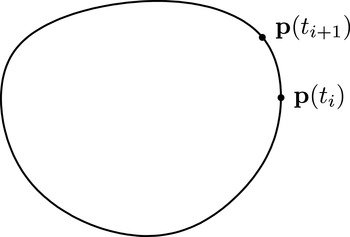
Schneider, Hormann and Floater (Reference Schneider, Hormann and Floater2013) proposed a solution to the injectivity problem using a sequence of intermediate polygons. If each consecutive pair of polygons are close enough to each other, we would expect a barycentric (MV) mapping between them to be injective, and by composing these individual mappings we thus obtain an injective mapping between the original two polygons.
Specifically, suppose, as in Section 4.4, that
 $P$
and
 $\tilde{P}$
are the two polygons of interest, with vertices
 $\boldsymbol{v}_{1},\ldots ,\boldsymbol{v}_{n}$
and
 $\tilde{\boldsymbol{v}}_{1},\ldots ,\tilde{\boldsymbol{v}}_{n}$
respectively. Suppose further that for each
 $i=1,\ldots ,n$
,
 $\boldsymbol{v}_{i}:[0,1]\rightarrow \mathbb{R}^{2}$
is a parametric curve connecting
 $\boldsymbol{v}_{i}$
to
 $\tilde{\boldsymbol{v}}_{i}$
, that is, with
 $\boldsymbol{v}_{i}(0)=\boldsymbol{v}_{i}$
and
 $\boldsymbol{v}_{i}(1)=\tilde{\boldsymbol{v}}_{i}$
. We assume that for each
 $t\in [0,1]$
, the vertices
 $\boldsymbol{v}_{1}(t),\ldots ,\boldsymbol{v}_{n}(t)$
form a valid polygon
 $P(t)$
. Then, choosing any partition of
 $[0,1]$
,
 $$\begin{eqnarray}0=t_{0}<t_{1}<\cdots <t_{m}=1,\end{eqnarray}$$
we can form a barycentric mapping
 $\mathbf{g}_{j}:P(t_{j})\rightarrow P(t_{j+1})$
via the formula
 $$\begin{eqnarray}\mathbf{g}_{j}(\mathbf{x})=\mathop{\sum }_{i=1}^{n}{\it\phi}_{i}(\mathbf{x};P(t_{j}))\boldsymbol{v}_{i}(t_{j+1}),\end{eqnarray}$$
where
 ${\it\phi}_{i}(\mathbf{x};P(t))$
is the
 $i$
th barycentric coordinate (for example MV) of the point
 $\mathbf{x}$
with respect to the polygon
 $P(t)$
. Then
 $$\begin{eqnarray}\mathbf{g}:=\mathbf{g}_{m-1}\circ \cdots \circ \mathbf{g}_{1}\circ \mathbf{g}_{0}\end{eqnarray}$$
is a mapping
 $P\rightarrow \tilde{P}$
, and numerical examples in Schneider et al. (Reference Schneider, Hormann and Floater2013) show that
 $\mathbf{g}$
is injective when the partition (5.9) is fine enough, that is, when the mesh size
 $h:=\max _{j=0,\ldots ,m-1}(t_{j+1}-t_{j})$
is small enough.
5.7. Limit of composite mappings
We will show that the above composite barycentric mapping is injective for a small enough mesh size
 $h$
by showing that its limit as
 $h\rightarrow 0$
satisfies a differential equation whose solution is indeed injective due to reversibility. This also confirms another feature of the mappings of Schneider et al. (Reference Schneider, Hormann and Floater2013), namely that reversing the direction of the composition appears to approximate the inverse of the composite mapping.
For a fixed
 $\mathbf{x}_{0}\in P$
, the mappings
 $\mathbf{g}_{j}$
in (5.10) define a sequence of points
 $\mathbf{x}_{1},\ldots ,\mathbf{x}_{m}$
, with
 $\mathbf{x}_{j+1}=\mathbf{g}_{j}(\mathbf{x}_{j})$
,
 $j=0,1,\ldots ,m-1$
. By equation (5.10),
 $$\begin{eqnarray}\mathbf{x}_{j+1}=\mathop{\sum }_{i=1}^{n}{\it\phi}_{i}(\mathbf{x}_{j};P(t_{j}))\boldsymbol{v}_{i}(t_{j+1}),\end{eqnarray}$$
and, on the other hand, by the barycentric property of the
 ${\it\phi}_{i}(\mathbf{x};P(t_{j}))$
,
 $$\begin{eqnarray}\mathbf{x}_{j}=\mathop{\sum }_{i=1}^{n}{\it\phi}_{i}(\mathbf{x}_{j};P(t_{j}))\boldsymbol{v}_{i}(t_{j}).\end{eqnarray}$$
The difference of these two equations is
 $$\begin{eqnarray}\mathbf{x}_{j+1}-\mathbf{x}_{j}=\mathop{\sum }_{i=1}^{n}{\it\phi}_{i}(\mathbf{x}_{j};P(t_{j}))(\boldsymbol{v}_{i}(t_{j+1})-\boldsymbol{v}_{i}(t_{j})),\end{eqnarray}$$
and dividing both sides by
 $t_{j+1}-t_{j}$
, and taking the limit as
 $t_{j+1}\rightarrow t_{j}$
yields the equation
 $$\begin{eqnarray}\mathbf{x}^{\prime }(t)=\mathop{\sum }_{i=1}^{n}{\it\phi}_{i}(\mathbf{x}(t);P(t))\boldsymbol{v}_{i}^{\prime }(t).\end{eqnarray}$$
This is a first-order equation (system) in the vector-valued function
 $\mathbf{x}(t)$
, with initial condition
 $\mathbf{x}(0)=\mathbf{x}_{0}$
, and has the form
 $$\begin{eqnarray}\mathbf{x}^{\prime }(t)=\mathbf{F}(t,\mathbf{x}(t)).\end{eqnarray}$$
Conditions for the local existence and uniqueness of the solution are well-studied, and from Picard–Lindelöf theory, it is sufficient that
 $\mathbf{F}(t,\mathbf{x})$
is Lipschitz-continuous as a function of
 $\mathbf{x}$
, which, from (5.12), is ensured if the coordinates
 ${\it\phi}_{i}$
are likewise Lipschitz-continuous with respect to
 $\mathbf{x}$
, which is the case for most of the coordinates we have studied. We can also see that there is a global solution
 $\mathbf{x}(t)$
since
 $\mathbf{x}(t)$
will remain inside the polygon
 $P(t)$
for all
 $t\in [0,1]$
. This is due to the boundary
 $\partial P(t)$
acting as a barrier. If the initial point
 $\mathbf{x}_{0}$
lies on an edge of the initial polygon
 $P$
, that is,
 $$\begin{eqnarray}\mathbf{x}_{0}=(1-{\it\mu})\boldsymbol{v}_{i}+{\it\mu}\boldsymbol{v}_{i+1},\end{eqnarray}$$
for some
 $i$
and some
 ${\it\mu}\in [0,1]$
, then the solution to (5.12) is
 $$\begin{eqnarray}\mathbf{x}(t)=(1-{\it\mu})\boldsymbol{v}_{i}(t)+{\it\mu}\boldsymbol{v}_{i+1}(t),\quad t\in [0,1],\end{eqnarray}$$
since differentiation gives
 $$\begin{eqnarray}\mathbf{x}^{\prime }(t)=(1-{\it\mu})\boldsymbol{v}_{i}^{\prime }(t)+{\it\mu}\boldsymbol{v}_{i+1}^{\prime }(t),\end{eqnarray}$$
which agrees with (5.12).
Observe also that the mapping
 $\mathbf{g}:P\rightarrow \tilde{P}$
defined by
 $\mathbf{g}(\mathbf{x}_{0})=\mathbf{x}(1)$
for each
 $\mathbf{x}_{0}\in P$
is injective due to the reversibility of (5.12). One can check that the solution to the reverse equation
 $$\begin{eqnarray}\mathbf{y}^{\prime }(t)=\mathop{\sum }_{i=1}^{n}{\it\phi}_{i}(\mathbf{y}(t);Q(t))\mathbf{w}_{i}^{\prime }(t),\end{eqnarray}$$
where
 $Q(t)=P(1-t)$
and
 $\mathbf{w}_{i}(t)=\boldsymbol{v}_{i}(1-t)$
, with initial condition
 $\mathbf{y}(0)=\mathbf{x}(1)$
, is
 $\mathbf{y}(t)=\mathbf{x}(1-t)$
. Therefore,
 $\mathbf{y}(1)=\mathbf{x}_{0}$
, and so
 $\mathbf{g}:P\rightarrow \tilde{P}$
has an inverse
 $\mathbf{g}^{-1}$
, generated by (5.13), with
 $\mathbf{g}^{-1}(\mathbf{x}(1))=\mathbf{x}_{0}$
.
We now see that the composite mapping (5.11) can be viewed as a numerical approximation to the mapping defined by the differential equation (5.12). The approximation is similar to Euler’s method, but also discretizes the derivative
 $\boldsymbol{v}_{i}^{\prime }(t)$
.
6. A general construction
In Floater et al. (Reference Floater, Hormann and Kós2006) the following general approach was used to construct barycentric coordinates for a convex polygon. We again use the fact that for each
 $i$
, the point
 $\mathbf{x}$
can be expressed as the linear combination (4.4) of the three vertices
 $\boldsymbol{v}_{i-1}$
,
 $\boldsymbol{v}_{i}$
,
 $\boldsymbol{v}_{i+1}$
. Recall that we used this fact to express the vector
 $\boldsymbol{v}_{i}-\mathbf{x}$
as a linear combination of
 $\boldsymbol{v}_{i}-\boldsymbol{v}_{i-1}$
and
 $\boldsymbol{v}_{i+1}-\boldsymbol{v}_{i}$
in (4.5), in order to construct Wachspress coordinates. Instead, we can use (4.4) to express
 $\boldsymbol{v}_{i}-\mathbf{x}$
as a linear combination of
 $\boldsymbol{v}_{i-1}-\mathbf{x}$
and
 $\boldsymbol{v}_{i+1}-\mathbf{x}$
:
 $$\begin{eqnarray}D_{i}(\mathbf{x}):=\frac{\boldsymbol{v}_{i-1}-\mathbf{x}}{A_{i-1}(\mathbf{x})}+\frac{\boldsymbol{v}_{i+1}-\mathbf{x}}{A_{i}(\mathbf{x})}-\frac{B_{i}(\mathbf{x})}{A_{i-1}(\mathbf{x})A_{i}(\mathbf{x})}(\boldsymbol{v}_{i}-\mathbf{x})=0.\end{eqnarray}$$
Thus any linear combination of the
 $D_{i}$
is zero,
 $$\begin{eqnarray}\mathop{\sum }_{i=1}^{n}c_{i}D_{i}=0,\end{eqnarray}$$
and by rearranging this sum, we deduce that the functions
 $$\begin{eqnarray}w_{i}=\frac{c_{i+1}A_{i-1}-c_{i}B_{i}+c_{i-1}A_{i}}{A_{i-1}A_{i}}\end{eqnarray}$$
satisfy
 $$\begin{eqnarray}\mathop{\sum }_{i}w_{i}(\mathbf{x})(\boldsymbol{v}_{i}-\mathbf{x})=0.\end{eqnarray}$$
Thus, if we can choose the
 $c_{i}$
, which may or not be functions of
 $\mathbf{x}$
, so that the
 $w_{i}$
are positive in
 $P$
,
 $$\begin{eqnarray}{\it\phi}_{i}:=w_{i}/\mathop{\sum }_{j=1}^{n}w_{j}\end{eqnarray}$$
are (positive) barycentric coordinates.
When
 $c_{i}=1$
, the coordinates
 ${\it\phi}_{i}$
in (6.2) are Wachspress, which easily follows from the fact that
 $$\begin{eqnarray}A_{i-1}+A_{i}=B_{i}+C_{i}.\end{eqnarray}$$
When
 $c_{i}=r_{i}:=\Vert \boldsymbol{v}_{i}-\mathbf{x}\Vert$
, the coordinates
 ${\it\phi}_{i}$
in (6.2) are MV. A third choice,
 $c_{i}=r_{i}^{2}$
, generates the ‘discrete harmonic coordinates’ of (5.7), that is, up to a scaling factor,
 $$\begin{eqnarray}w_{i}=\cot ({\it\alpha}_{i})+\cot ({\it\beta}_{i}),\end{eqnarray}$$
with
 ${\it\alpha}_{i}$
the angle at
 $\boldsymbol{v}_{i-1}$
of the triangle
 $[\mathbf{x},\boldsymbol{v}_{i-1},\boldsymbol{v}_{i}]$
and
 ${\it\beta}_{i}$
the angle at
 $\boldsymbol{v}_{i+1}$
of the triangle
 $[\mathbf{x},\boldsymbol{v}_{i},\boldsymbol{v}_{i+1}]$
. While the sum
 $\sum _{j=1}^{n}w_{j}$
is positive in
 $P$
, the only case in which all the individual weights
 $w_{i}$
are positive is when the vertices of
 $P$
lie on a circle. Interestingly, in this special circle case, the discrete harmonic coordinates are equal to the Wachspress coordinates.
Various other choices of the
 $c_{i}$
which generate positive coordinates
 ${\it\phi}_{i}$
were found in Floater et al. (Reference Floater, Hormann and Kós2006). We will now show that for quadrilaterals, the inverse bilinear coordinates of Section 3 also fit into this general framework.
Theorem 6.1. With
 $n=4$
, if
 $c_{i}=C_{i}+\sqrt{D}$
, with
 $D$
as in (3.3), the coordinates
 ${\it\phi}_{i}$
in (6.2) are inverse bilinear.
Proof. By Theorem 3.1, we can express the inverse bilinear
 ${\it\phi}_{i}$
as (6.2), where
 $$\begin{eqnarray}w_{i}=\frac{E_{i-1}E_{i}}{A_{i-1}A_{i}},\quad i=1,2,3,4.\end{eqnarray}$$
Now an algebraic computation shows that
 $$\begin{eqnarray}E_{i-1}E_{i}=2(c_{i+1}A_{i-1}-c_{i}B_{i}+c_{i-1}A_{i}),\end{eqnarray}$$
where
 $c_{i}=C_{i}+\sqrt{D}$
.☐
For a general convex
 $n$
-gon, Theorem 6.1 inspires other choices of generating weights
 $c_{i}$
, as follows.
Theorem 6.2. For any
 $n\geq 3$
, let
 $c_{i}=C_{i}+S$
, where
 $S:P\rightarrow \mathbb{R}$
is any function such that
 $S\geq \max _{i}B_{i}$
on
 $P$
. Then the coordinates
 ${\it\phi}_{i}$
in (6.2) are positive.
Proof. With this choice of
 $c_{i}$
,
 $w_{i}$
in (6.1) becomes
 $$\begin{eqnarray}\hspace{60.00009pt}w_{i}=\frac{C_{i+1}A_{i-1}+C_{i}(S-B_{i})+C_{i-1}A_{i}}{A_{i-1}A_{i}}>0.\hspace{60.00009pt}\Box\end{eqnarray}$$
Observe further that if
 $S$
is constant in
 $\mathbf{x}$
, then the numerator of
 $w_{i}$
is linear in
 $\mathbf{x}$
, and so
 ${\it\phi}_{i}$
is a rational function, degree
 $n-1$
over degree
 $n-2$
, only one degree higher than Wachspress coordinates. As an example, we could let
 $S=A(P)$
, the area of
 $P$
, or
 $$\begin{eqnarray}S=\max _{i}\max _{j\neq i-1,i,i+1}A(\boldsymbol{v}_{j},\boldsymbol{v}_{i-1},\boldsymbol{v}_{i+1}).\end{eqnarray}$$
7. Maximum entropy coordinates
These coordinates were developed by Sukumar (Reference Sukumar2004) and Hormann and Sukumar (Reference Hormann and Sukumar2008). Sukumar (Reference Sukumar2004) suggested finding positive barycentric coordinates
 ${\it\phi}_{1},\ldots ,{\it\phi}_{n}$
for a fixed point
 $\mathbf{x}$
in a convex
 $n$
-gon
 $P$
by maximizing the ‘entropy’
 $$\begin{eqnarray}H({\it\phi}_{1},\ldots ,{\it\phi}_{n}):=-\mathop{\sum }_{i=1}^{n}{\it\phi}_{i}\log ({\it\phi}_{i}),\end{eqnarray}$$
subject to the linear constraints (2.1). Using Lagrange multipliers he showed that the solution is
 $$\begin{eqnarray}{\it\phi}_{i}=w_{i}/W,\quad W=\mathop{\sum }_{j=1}^{n}w_{j},\end{eqnarray}$$
with
 $$\begin{eqnarray}w_{i}=\text{e}^{\boldsymbol{{\it\lambda}}\cdot \mathbf{d}_{i}},\end{eqnarray}$$
and
 $\mathbf{d}_{i}=\boldsymbol{v}_{i}-\mathbf{x}$
, and where the vector
 $\boldsymbol{{\it\lambda}}\in \mathbb{R}^{2}$
is such that (4.3) holds, which is equivalent to finding
 $\boldsymbol{{\it\lambda}}\in \mathbb{R}^{2}$
such that
 $$\begin{eqnarray}\mathop{\sum }_{i=1}^{n}\text{e}^{\boldsymbol{{\it\lambda}}\cdot \mathbf{d}_{i}}\mathbf{d}_{i}=0.\end{eqnarray}$$
One can show that this equation has a unique solution
 $\boldsymbol{{\it\lambda}}$
and so this method yields positive barycentric coordinates, and by the convexity of the polygon, they have the Lagrange property on the boundary of the polygon. Lee (Reference Lee1990) mentions the existence and uniqueness of such coordinates for convex polytopes, but without computational details.
This method also generates positive barycentric coordinates for an arbitrary
 $n$
-gon
 $P$
, but without the Lagrange property at the boundary. In a later development, Hormann and Sukumar (Reference Hormann and Sukumar2008) generalized the method to use ‘priors’, that is, positive weights
 $m_{i}>0$
,
 $i=1,\ldots ,n$
, and showed that with an appropriate choice of priors, the method then generates positive barycentric coordinates with the Lagrange property.
Consider the latter situation in which
 $P$
is an arbitrary
 $n$
-gon,
 $\mathbf{x}$
is some fixed point inside it, and positive values, ‘priors’,
 $m_{1},\ldots ,m_{n}>0$
have been chosen. The method then reduces to finding
 ${\it\phi}_{1},\ldots ,{\it\phi}_{n}$
of the form (7.1) with
 $$\begin{eqnarray}w_{i}=m_{i}\,\text{e}^{\boldsymbol{{\it\lambda}}\cdot \mathbf{d}_{i}},\end{eqnarray}$$
and with
 $\boldsymbol{{\it\lambda}}\in \mathbb{R}^{2}$
the solution to
 $$\begin{eqnarray}\mathop{\sum }_{i=1}^{n}m_{i}\,\text{e}^{\boldsymbol{{\it\lambda}}\cdot \mathbf{d}_{i}}\mathbf{d}_{i}=0.\end{eqnarray}$$
To see that (7.3) has a unique solution
 $\boldsymbol{{\it\lambda}}$
, observe that it is equivalent to the equation
 $$\begin{eqnarray}{\rm\nabla}F(\boldsymbol{{\it\lambda}})=0,\end{eqnarray}$$
where
 $F:\mathbb{R}^{2}\rightarrow \mathbb{R}$
is the function
 $$\begin{eqnarray}F(\boldsymbol{{\it\lambda}})=\mathop{\sum }_{i=1}^{n}m_{i}\,\text{e}^{\boldsymbol{{\it\lambda}}\cdot \mathbf{d}_{i}}.\end{eqnarray}$$
This means that (7.3) has a unique solution if
 $F$
is a strictly convex function, in which case
 $\boldsymbol{{\it\lambda}}$
in (7.3) is its unique minimum. To see that
 $F$
is indeed strictly convex, we follow the analysis of Sukumar (Reference Sukumar2004) and observe that the Hessian matrix of
 $F$
is
 $$\begin{eqnarray}H(F)=\left[\begin{array}{@{}cc@{}}\mathop{\sum }_{i}m_{i}\,\text{e}^{\boldsymbol{{\it\lambda}}\cdot \mathbf{d}_{i}}d_{i}^{2} & \mathop{\sum }_{i}m_{i}\,\text{e}^{\boldsymbol{{\it\lambda}}\cdot \mathbf{d}_{i}}d_{i}e_{i}\\ \mathop{\sum }_{i}m_{i}\,\text{e}^{\boldsymbol{{\it\lambda}}\cdot \mathbf{d}_{i}}d_{i}e_{i} & \mathop{\sum }_{i}m_{i}\,\text{e}^{\boldsymbol{{\it\lambda}}\cdot \mathbf{d}_{i}}e_{i}^{2}\end{array}\right]\!,\end{eqnarray}$$
where
 $\mathbf{d}_{i}=(d_{i},e_{i})$
. Defining
 $a_{i}=(m_{i}\,\text{e}^{\boldsymbol{{\it\lambda}}\cdot \mathbf{d}_{i}})^{1/2}$
,
 $i=1,\ldots ,n$
, and
 $$\begin{eqnarray}\mathbf{U}=(a_{1}d_{1},\ldots ,a_{n}d_{n}),\quad \mathbf{V}=(a_{1}e_{1},\ldots ,a_{n}e_{n}),\end{eqnarray}$$
we can express
 $H(F)$
as
 $$\begin{eqnarray}\left[\begin{array}{@{}cc@{}}\Vert \mathbf{U}\Vert ^{2} & \mathbf{U}\cdot \mathbf{V}\\ \mathbf{U}\cdot \mathbf{V} & \Vert \mathbf{V}\Vert ^{2}\end{array}\right]\!,\end{eqnarray}$$
with
 $\Vert \cdot \Vert$
the Euclidean norm in
 $\mathbb{R}^{n}$
, and therefore, by the Cauchy–Schwarz inequality,
 $\det (H(F))\geq 0$
, with equality if and only if the vectors
 $\mathbf{U}$
and
 $\mathbf{V}$
are parallel. These vectors cannot be parallel since this would imply that all the vertices
 $\boldsymbol{v}_{i}$
of
 $P$
lie on some straight line through the point
 $\mathbf{x}$
. Thus
 $\det (H(F))>0$
and since
 $H(F)$
also has positive diagonal elements, we conclude that
 $H(F)$
is strictly positive definite and that
 $F$
is strictly convex, and that (7.3) does indeed have a unique solution
 $\boldsymbol{{\it\lambda}}$
.
How do we choose priors
 $m_{i}$
, as functions of
 $\mathbf{x}$
in
 $P$
and extended to
 $\mathbf{x}\in \partial P$
, to ensure that the resulting coordinates
 ${\it\phi}_{i}$
have the Lagrange property on
 $\partial P$
? Due to the form of
 $w_{i}$
in (7.2) it is sufficient to choose the
 $m_{i}$
so that
 $m_{i}(\boldsymbol{v}_{i})\neq 0$
and for
 $\mathbf{x}\in [\boldsymbol{v}_{i},\boldsymbol{v}_{i+1}]$
,
 $m_{j}(\mathbf{x})=0$
for
 $j\neq i,i+1$
. Hormann and Sukumar (Reference Hormann and Sukumar2008) gave the following solution. To the edge
 $[\boldsymbol{v}_{i},\boldsymbol{v}_{i+1}]$
of
 $P$
they associate the edge weight function
 $$\begin{eqnarray}{\it\rho}_{i}(\mathbf{x})=\Vert \mathbf{x}-\boldsymbol{v}_{i}\Vert +\Vert \mathbf{x}-\boldsymbol{v}_{i+1}\Vert -\Vert \boldsymbol{v}_{i}-\boldsymbol{v}_{i+1}\Vert ,\end{eqnarray}$$
which is non-negative and vanishes only on the edge itself. They then let
 $$\begin{eqnarray}{\it\pi}_{i}=\mathop{\prod }_{j\neq i-1,i}{\it\rho}_{j},\end{eqnarray}$$
and
 $$\begin{eqnarray}m_{i}={\it\pi}_{i}\Big/\mathop{\sum }_{j=1}^{n}{\it\pi}_{j}.\end{eqnarray}$$
Another solution is to take the edge weight
 $$\begin{eqnarray}{\it\rho}_{i}(\mathbf{x})=\Vert \mathbf{x}-\boldsymbol{v}_{i}\Vert \Vert \mathbf{x}-\boldsymbol{v}_{i+1}\Vert +(\mathbf{x}-\boldsymbol{v}_{i})\cdot (\mathbf{x}-\boldsymbol{v}_{i+1}).\end{eqnarray}$$
8. Coordinates in higher dimensions
So far we have only considered coordinates for points in
 $\mathbb{R}^{2}$
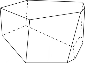
, but there are applications of barycentric coordinates for points in a polyhedron in
 $\mathbb{R}^{3}$
, such as in Figure 8.1, or more generally for points in a polytope in
 $\mathbb{R}^{d}$
. Both Wachspress and MV coordinates have been generalized to higher dimensions.
Simple, convex polyhedron.

8.1. Wachspress coordinates in three dimensions
Wachspress (Reference Wachspress1975, Chapter 7), and Warren (Reference Warren1996) constructed rational coordinates for simple convex polyhedra: convex polyhedra in which all vertices have three incident faces. Warren et al. (Reference Warren, Schaefer, Hirani and Desbrun2007) derived the same coordinates in a different way, avoiding the ‘adjoint’, generalizing (4.8) as follows. Let
 $P\subset \mathbb{R}^{3}$
be a simple convex polyhedron, with faces
 $F$
and vertices
 $V$
. For each face
 $f\in F$
, let
 $\mathbf{n}_{f}\in \mathbb{R}^{3}$
denote its unit outward normal, and for any
 $\mathbf{x}\in P$
, let
 $h_{f}(\mathbf{x})$
denote the perpendicular distance of
 $\mathbf{x}$
to
 $f$
, which can be expressed as the scalar product
 $$\begin{eqnarray}h_{f}(\mathbf{x})=(\boldsymbol{v}-\mathbf{x})\cdot \mathbf{n}_{f},\end{eqnarray}$$
for any vertex
 $\boldsymbol{v}\in V$
belonging to
 $f$
. For each vertex
 $\boldsymbol{v}\in V$
, let
 $f_{1},f_{2},f_{3}$
be the three faces incident to
 $\boldsymbol{v}$
, and for
 $\mathbf{x}\in P$
, let
 $$\begin{eqnarray}w_{\boldsymbol{v}}(\mathbf{x})=\frac{\det (\mathbf{n}_{f_{1}},\mathbf{n}_{f_{2}},\mathbf{n}_{f_{3}})}{h_{f_{1}}(\mathbf{x})h_{f_{2}}(\mathbf{x})h_{f_{3}}(\mathbf{x})},\end{eqnarray}$$
where it is understood that
 $f_{1},f_{2},f_{3}$
are ordered such that the determinant in the numerator is positive. Here, for vectors
 $\mathbf{a},\mathbf{b},\mathbf{c}\in \mathbb{R}^{3}$
,
 $$\begin{eqnarray}\det (\mathbf{a},\mathbf{b},\mathbf{c}):=\left|\begin{array}{@{}ccc@{}}a_{1} & b_{1} & c_{1}\\ a_{2} & b_{2} & c_{2}\\ a_{3} & b_{3} & c_{3}\end{array}\right|\!.\end{eqnarray}$$
Thus the ordering of
 $f_{1},f_{2},f_{3}$
must be anticlockwise around
 $\boldsymbol{v}$
, seen from outside
 $P$
. In this way,
 $w_{\boldsymbol{v}}(\mathbf{x})>0$
, and it was shown in Warren et al. (Reference Warren, Schaefer, Hirani and Desbrun2007) that the functions
 $$\begin{eqnarray}{\it\phi}_{\boldsymbol{v}}(\mathbf{x}):=\frac{w_{\boldsymbol{v}}(\mathbf{x})}{\mathop{\sum }_{\mathbf{u}\in V}w_{\mathbf{u}}(\mathbf{x})}\end{eqnarray}$$
are barycentric coordinates for
 $\mathbf{x}\in P$
in the sense that
 $$\begin{eqnarray}\mathop{\sum }_{\boldsymbol{v}\in V}{\it\phi}_{\boldsymbol{v}}(\mathbf{x})=1,\quad \mathop{\sum }_{\boldsymbol{v}\in V}{\it\phi}_{\boldsymbol{v}}(\mathbf{x})\boldsymbol{v}=\mathbf{x}.\end{eqnarray}$$
To deal with non-simple polyhedra, it was suggested in Warren et al. (Reference Warren, Schaefer, Hirani and Desbrun2007) that one might decompose a non-simple vertex into simple ones by perturbing its adjacent facets. Later, Ju et al. (Reference Ju, Schaefer, Warren and Desbrun2005b
) found a cleaner solution, using properties of the so-called polar dual. With respect to each
 $\mathbf{x}$
in a general convex polyhedron
 $P\subset \mathbb{R}^{3}$
, there is a dual polyhedron,
 $$\begin{eqnarray}\tilde{P}_{\mathbf{x}}:=\{\mathbf{y}\in \mathbb{R}^{3}:\mathbf{y}\cdot (\mathbf{z}-\mathbf{x})\leq 1,\mathbf{z}\in P\}.\end{eqnarray}$$
It contains the origin
 $\mathbf{y}=0$
, and its vertices are the endpoints of the vectors
 $$\begin{eqnarray}\mathbf{p}_{f}(\mathbf{x}):=\frac{\mathbf{n}_{f}}{h_{f}(\mathbf{x})},\quad f\in F,\end{eqnarray}$$
when placed at the origin. Suppose that a vertex
 $\boldsymbol{v}\in V$
has
 $k$
incident faces,
 $f_{1},\ldots ,f_{k}$
, for some
 $k\geq 3$
, where we again assume they are ordered in some anticlockwise fashion around
 $\boldsymbol{v}$
, as seen from outside
 $P$
. The endpoints of the
 $k$
vectors
 $\mathbf{p}_{f_{1}}(\mathbf{x}),\ldots \mathbf{p}_{f_{k}}(\mathbf{x})$
form a
 $k$
-sided polygon. This polygon is the face of
 $\tilde{P}_{\mathbf{x}}$
, dual to the vertex
 $\boldsymbol{v}$
of
 $P$
. This face and the origin in
 $\mathbb{R}^{3}$
form a polygonal pyramid,
 $Q_{\boldsymbol{v}}\subset \tilde{P}_{\mathbf{x}}$
. It was shown in Ju et al. (Reference Ju, Schaefer, Warren and Desbrun2005b
) that if we define
 $$\begin{eqnarray}w_{\boldsymbol{v}}(\mathbf{x})=\text{vol}(Q_{\boldsymbol{v}}),\end{eqnarray}$$
then the functions
 ${\it\phi}_{\boldsymbol{v}}$
in (8.1) are again barycentric coordinates. This follows from the fact that the integral of all unit normals to the dual polyhedron is zero. In practice we could triangulate the face dual to
 $\boldsymbol{v}$
by connecting the endpoint of
 $\mathbf{p}_{f_{k}}(\mathbf{x})$
to the endpoints of all the other
 $\mathbf{p}_{f_{i}}(\mathbf{x})$
, and so compute
 $\text{vol}(Q_{\boldsymbol{v}})$
as a sum of volumes of tetrahedra. Thus, we could let
 $$\begin{eqnarray}w_{\boldsymbol{v}}(\mathbf{x})=\mathop{\sum }_{i=1}^{k-2}w_{i,\boldsymbol{v}}(\mathbf{x}),\quad \text{where}\quad w_{i,\boldsymbol{v}}(\mathbf{x})=\det (\mathbf{p}_{f_{i}}(\mathbf{x}),\mathbf{p}_{f_{i+1}}(\mathbf{x}),\mathbf{p}_{f_{k}}(\mathbf{x})).\end{eqnarray}$$
8.2. Gradients
From the above formula for
 $w_{\boldsymbol{v}}$
, one can show that
 $$\begin{eqnarray}{\rm\nabla}w_{\boldsymbol{v}}=\mathop{\sum }_{i=1}^{k-2}w_{i,\boldsymbol{v}}(\mathbf{p}_{f_{i}}+\mathbf{p}_{f_{i+1}}+\mathbf{p}_{f_{k}}),\end{eqnarray}$$
from which we can find the ratio
 $\mathbf{R}_{\boldsymbol{v}}:={\rm\nabla}w_{\boldsymbol{v}}/w_{\boldsymbol{v}}$
, and then the gradient of
 ${\it\phi}_{\boldsymbol{v}}$
can be computed by the formula
 $$\begin{eqnarray}{\rm\nabla}{\it\phi}_{\boldsymbol{v}}={\it\phi}_{\boldsymbol{v}}\biggl(\mathbf{R}_{\boldsymbol{v}}-\mathop{\sum }_{\mathbf{u}\in V}{\it\phi}_{\mathbf{u}}\mathbf{R}_{\mathbf{u}}\biggr).\end{eqnarray}$$
This was derived in Floater et al. (Reference Floater, Gillette and Sukumar2014), where some MATLAB™ code for evaluating
 ${\it\phi}_{\boldsymbol{v}}$
and
 ${\rm\nabla}{\it\phi}_{\boldsymbol{v}}$
can also be found.
8.3. MV coordinates in three dimensions
MV coordinates were generalized to three dimensions in Floater et al. (Reference Floater, Kos and Reimers2005) and Ju et al. (Reference Ju, Schaefer and Warren2005a ), the basic idea being to replace integration over the unit circle, as in Section 5, by integration over the unit sphere.
Consider first the case that
 $P\subset \mathbb{R}^{3}$
is a convex polyhedron with triangular faces, though it does not need to be simple. Fix
 $\mathbf{x}\in P$
and consider the radial projection of the boundary of
 $P$
onto the unit sphere centred at
 $\mathbf{x}$
. A vertex
 $\boldsymbol{v}\in V$
is projected to the point (unit vector)
 $\mathbf{e}_{\boldsymbol{v}}:=(\boldsymbol{v}-\mathbf{x})/\Vert \boldsymbol{v}-\mathbf{x}\Vert$
. A face
 $f\in F$
is projected to a spherical triangle
 $f_{\mathbf{x}}$
whose vertices are
 $\mathbf{e}_{\boldsymbol{v}}$
,
 $\boldsymbol{v}\in V_{f}$
, where
 $V_{f}\subset V$
denotes the set of (three) vertices of
 $f$
. Let
 $\mathbf{I}_{f}$
denote the (vector-valued) integral of its unit normals,
 $$\begin{eqnarray}\mathbf{I}_{f}:=\int _{f_{\mathbf{x}}}\mathbf{n}(\mathbf{y})\,\text{d}\mathbf{y}.\end{eqnarray}$$
Since the three vectors
 $\mathbf{e}_{\boldsymbol{v}}$
,
 $\boldsymbol{v}\in V_{f}$
, are linearly independent, there are three unique weights
 $w_{\boldsymbol{v},f}>0$
such that
 $$\begin{eqnarray}\mathbf{I}_{f}=\mathop{\sum }_{\boldsymbol{v}\in V_{f}}w_{\boldsymbol{v},f}\mathbf{e}_{\boldsymbol{v}}.\end{eqnarray}$$
The weights can be found as ratios of
 $3\times 3$
determinants from Cramer’s rule. Since the integral of all unit normals of the unit sphere is zero, and letting
 $F_{\boldsymbol{v}}\subset F$
denote the set of faces that are incident on the vertex
 $\boldsymbol{v}$
, we find, by switching summations, that
 $$\begin{eqnarray}0=\mathop{\sum }_{f\in F}\mathbf{I}_{f}=\mathop{\sum }_{f\in F}\mathop{\sum }_{\boldsymbol{v}\in V_{f}}w_{\boldsymbol{v},f}\mathbf{e}_{\boldsymbol{v}}=\mathop{\sum }_{\boldsymbol{v}\in V}\mathop{\sum }_{f\in F_{\boldsymbol{v}}}w_{\boldsymbol{v},f}\mathbf{e}_{\boldsymbol{v}},\end{eqnarray}$$
and so the functions
 $$\begin{eqnarray}w_{\boldsymbol{v}}(\mathbf{x}):=\mathop{\sum }_{f\in F_{\boldsymbol{v}}}\frac{w_{\boldsymbol{v},f}(\mathbf{x})}{\Vert \boldsymbol{v}-\mathbf{x}\Vert }\end{eqnarray}$$
satisfy
 $$\begin{eqnarray}\mathop{\sum }_{\boldsymbol{v}\in V}w_{\boldsymbol{v}}(\mathbf{x})(\boldsymbol{v}-\mathbf{x})=0.\end{eqnarray}$$
It follows that the functions
 ${\it\phi}_{\boldsymbol{v}}$
given by (8.1) with
 $w_{\boldsymbol{v}}$
given by (8.4) are barycentric coordinates, that is, they are positive in
 $P$
and satisfy (8.2).
It remains to find the integral
 $\mathbf{I}_{f}$
in terms of the points
 $\boldsymbol{v}\in V_{f}$
and
 $\mathbf{x}$
. We follow the observation made in Floater et al. (Reference Floater, Kos and Reimers2005). The spherical triangle
 $f_{\mathbf{x}}$
and the point
 $\mathbf{x}$
form a wedge of the unit ball centred at
 $\mathbf{x}$
. Since the integral of all unit normals over the surface of this wedge is zero, the integral
 $\mathbf{I}_{f}$
is minus the sum of the integrals over the three planar faces of the wedge. Suppose
 $\boldsymbol{v}_{1},\boldsymbol{v}_{2},\boldsymbol{v}_{3}$
are the vertices of
 $f$
in anticlockwise order, and let
 $\mathbf{e}_{i}=\mathbf{e}_{\boldsymbol{v}_{i}}$
. For
 $i=1,2,3$
, the
 $i$
th side of the wedge is the sector of the unit disk formed by the two unit vectors
 $\mathbf{e}_{i}$
and
 $\mathbf{e}_{i+1}$
, with the cyclic notation
 $\boldsymbol{v}_{i+3}:=\boldsymbol{v}_{i}$
. If
 ${\it\beta}_{i}\in (0,{\it\pi})$
is the angle between
 $\mathbf{e}_{i}$
and
 $\mathbf{e}_{i+1}$
then the area of the sector is
 ${\it\beta}_{i}/2$
, and hence
 $$\begin{eqnarray}\mathbf{I}_{f}=\frac{1}{2}\mathop{\sum }_{i=1}^{3}{\it\beta}_{i}\mathbf{m}_{i},\end{eqnarray}$$
where
 $$\begin{eqnarray}\mathbf{m}_{i}=\frac{\mathbf{e}_{i}\times \mathbf{e}_{i+1}}{\Vert \mathbf{e}_{i}\times \mathbf{e}_{i+1}\Vert }.\end{eqnarray}$$
Equating this with (8.3) gives
 $$\begin{eqnarray}w_{\boldsymbol{v}_{i},f}=\frac{1}{2}\mathop{\sum }_{j=1}^{3}{\it\beta}_{j}\frac{\mathbf{m}_{j}\cdot \mathbf{m}_{i+1}}{\mathbf{e}_{i}\cdot \mathbf{m}_{i+1}}.\end{eqnarray}$$
These three-dimensional MV coordinates were used for surface deformation by Ju et al. (Reference Ju, Schaefer and Warren2005a ) when the surface is represented as a dense triangular mesh. Some contour plots of the coordinate functions can be found in Floater et al. (Reference Floater, Kos and Reimers2005).
For a polyhedron with faces having arbitrary numbers of vertices, the same approach can be applied, but there is no longer uniqueness. Suppose
 $f\in F$
is a face with
 $k\geq 3$
vertices. The integral
 $\mathbf{I}_{f}$
is again well-defined, and can be computed as the sum of
 $k$
terms, generalizing (8.5). However, there is no unique choice of the local weights
 $w_{\boldsymbol{v},f}$
in (8.3) for
 $k>3$
, since there are
 $k$
of these. Langer, Belyaev and Seidel (Reference Langer, Belyaev and Seidel2006) suggested choosing the
 $w_{\boldsymbol{v},f}$
to be spherical MV coordinates, though one could also choose, for example, spherical Wachspress coordinates; see Section 9.
9. Spherical coordinates
Spherical barycentric coordinates for points in a spherical triangle were studied by Möbius (Reference Möbius1846, Section 14) and Alfeld, Neamtu and Schumaker (Reference Alfeld, Neamtu and Schumaker1996), and used in the latter to develop spherical Bernstein–Bézier polynomials. This motivates the study of generalizations of such coordinates to convex spherical polygons. Langer et al. (Reference Langer, Belyaev and Seidel2006) did that, and also pointed out how such coordinates can be applied to construct three-dimensional MV coordinates for polyhedra with polygonal faces, as in Section 8.3.
Consider first a spherical triangle
 $T$
on the unit sphere, with the unit vectors
 $\boldsymbol{v}_{1},\boldsymbol{v}_{2},\boldsymbol{v}_{3}\in \mathbb{R}^{3}$
as its vertices, and let
 $\mathbf{x}\in T$
. Since
 $\boldsymbol{v}_{1}$
,
 $\boldsymbol{v}_{2}$
,
 $\boldsymbol{v}_{3}$
are linearly independent, there exist unique values
 ${\it\phi}_{1},{\it\phi}_{2},{\it\phi}_{3}\in \mathbb{R}$
such that
 $$\begin{eqnarray}\mathbf{x}=\mathop{\sum }_{i=1}^{3}{\it\phi}_{i}\boldsymbol{v}_{i}.\end{eqnarray}$$
By Cramer’s rule, these values, which we will call the spherical barycentric coordinates of
 $\mathbf{x}$
, are
 $$\begin{eqnarray}{\it\phi}_{1}=\frac{\det (\mathbf{x},\boldsymbol{v}_{2},\boldsymbol{v}_{3})}{\det (\boldsymbol{v}_{1},\boldsymbol{v}_{2},\boldsymbol{v}_{3})},\quad {\it\phi}_{2}=\frac{\det (\boldsymbol{v}_{1},\mathbf{x},\boldsymbol{v}_{3})}{\det (\boldsymbol{v}_{1},\boldsymbol{v}_{2},\boldsymbol{v}_{3})},\quad {\it\phi}_{3}=\frac{\det (\boldsymbol{v}_{1},\boldsymbol{v}_{2},\mathbf{x})}{\det (\boldsymbol{v}_{1},\boldsymbol{v}_{2},\boldsymbol{v}_{3})},\end{eqnarray}$$
and they are positive. Unlike in the case of a planar triangle, spherical barycentric coordinates do not in general sum to 1. By the triangle inequality,
 $$\begin{eqnarray}\mathop{\sum }_{i=1}^{3}{\it\phi}_{i}=\mathop{\sum }_{i=1}^{3}{\it\phi}_{i}\Vert \boldsymbol{v}_{i}\Vert \geq \Vert \mathbf{x}\Vert =1,\end{eqnarray}$$
with equality only in the case that
 $\mathbf{x}=\boldsymbol{v}_{i}$
for some
 $i$
, in which case
 ${\it\phi}_{i}=1$
and
 ${\it\phi}_{j}=0$
,
 $j\neq i$
. For more details and other formulas we refer the reader to Alfeld et al. (Reference Alfeld, Neamtu and Schumaker1996).
Consider next a convex spherical polygon
 $P$
whose vertices are the unit vectors
 $\boldsymbol{v}_{1},\ldots ,\boldsymbol{v}_{n}\in \mathbb{R}^{3}$
,
 $n\geq 3$
, which, for the sake of simplicity, we assume are ordered anticlockwise, viewed from outside the sphere. We make the implicit assumption here that all the vertices
 $\boldsymbol{v}_{i}$
lie in some hemisphere, i.e., that there is some unit vector
 $\boldsymbol{v}_{0}\in \mathbb{R}^{3}$
such that
 $$\begin{eqnarray}\boldsymbol{v}_{i}\cdot \boldsymbol{v}_{0}>0,\quad i=1,\ldots ,n.\end{eqnarray}$$
This further means that for any
 $\mathbf{x}\in P$
and for any vertex
 $\boldsymbol{v}_{i}$
, the geodesic (a great circular arc) between
 $\mathbf{x}$
and
 $\boldsymbol{v}_{i}$
lies inside
 $P$
, even though
 $\boldsymbol{v}_{i}\cdot \mathbf{x}$
may be positive, zero, or negative, or equivalently, the angle
 ${\it\theta}_{i}\in (0,{\it\pi})$
between
 $\boldsymbol{v}_{i}$
and
 $\mathbf{x}$
may be less than, equal to, or greater than
 ${\it\pi}/2$
.
Given
 $\mathbf{x}\in P$
, we call any positive values
 ${\it\phi}_{1},\ldots ,{\it\phi}_{n}$
generalized spherical barycentric coordinates if
 $$\begin{eqnarray}\mathbf{x}=\mathop{\sum }_{i=1}^{n}{\it\phi}_{i}\boldsymbol{v}_{i}.\end{eqnarray}$$
How might we find such coordinates? Langer et al. (Reference Langer, Belyaev and Seidel2006) proposed using a projection: projecting
 $P$
radially from the origin to the tangent plane to the sphere at
 $\mathbf{x}$
. One can then use some known planar barycentric coordinates to express
 $\mathbf{x}$
as a linear combination of the projected vertices, and afterwards convert the expression to the form (9.1). This works when
 $\boldsymbol{v}_{i}\cdot \mathbf{x}>0$
for all
 $i$
, but if
 $\boldsymbol{v}_{i}\cdot \mathbf{x}\leq 0$
for some of the
 $i$
, the projected vertices will not form a valid planar polygon. The following alternative approach, based on the vector cross products
 $\boldsymbol{v}_{i}\times \mathbf{x}$
, works regardless of the signs of the
 $\boldsymbol{v}_{i}\cdot \mathbf{x}$
and results in the same coordinates as those of Langer et al. (Reference Langer, Belyaev and Seidel2006) in the case that
 $\boldsymbol{v}_{i}\cdot \mathbf{x}>0$
for all
 $i$
.
Lemma 9.1. For
 $\mathbf{x}\in P$
, suppose there are weights
 $w_{1},\ldots ,w_{n}>0$
such that
 $$\begin{eqnarray}\mathop{\sum }_{i=1}^{n}w_{i}\boldsymbol{v}_{i}\times \mathbf{x}=\mathbf{0}.\end{eqnarray}$$
Then the values
 $$\begin{eqnarray}{\it\phi}_{i}=w_{i}\Big/\mathop{\sum }_{j=1}^{n}w_{j}\boldsymbol{v}_{j}\cdot \mathbf{x},\quad i=1,\ldots ,n,\end{eqnarray}$$
are spherical barycentric coordinates for
 $\mathbf{x}$
.
Proof. Equation (9.2) implies that the vector
 $\boldsymbol{v}:=\sum _{i=1}^{n}w_{i}\boldsymbol{v}_{i}$
is parallel to the vector
 $\mathbf{x}$
, and since the
 $w_{i}$
are positive,
 $\boldsymbol{v}\cdot \mathbf{x}>0$
, and therefore
 $$\begin{eqnarray}\hspace{90.00014pt}\mathbf{x}=\boldsymbol{v}/\Vert \boldsymbol{v}\Vert =\boldsymbol{v}/(\boldsymbol{v}\cdot \mathbf{x}).\hspace{120.00018pt}\Box\end{eqnarray}$$
9.1. Spherical Wachspress coordinates
One choice of the weights
 $w_{i}$
in (9.2) can be derived in an analogous way to planar Wachspress coordinates, with (9.2) playing the role of (4.3).
Theorem 9.2. For
 $\mathbf{x}\in P$
, the values
 $$\begin{eqnarray}{\it\phi}_{i}=\frac{w_{i}}{\mathop{\sum }_{j=1}^{n}w_{j}\boldsymbol{v}_{j}\cdot \mathbf{x}},\quad w_{i}=\frac{\det (\boldsymbol{v}_{i-1},\boldsymbol{v}_{i},\boldsymbol{v}_{i+1})}{\det (\mathbf{x},\boldsymbol{v}_{i-1},\boldsymbol{v}_{i})\det (\mathbf{x},\boldsymbol{v}_{i},\boldsymbol{v}_{i+1})},\end{eqnarray}$$
are spherical barycentric coordinates for
 $\mathbf{x}$
.
Proof. Let
 $$\begin{eqnarray}A_{i}=\det (\mathbf{x},\boldsymbol{v}_{i},\boldsymbol{v}_{i+1}),\quad B_{i}=\det (\mathbf{x},\boldsymbol{v}_{i-1},\boldsymbol{v}_{i+1}),\end{eqnarray}$$
and
 $$\begin{eqnarray}C_{i}=\det (\boldsymbol{v}_{i-1},\boldsymbol{v}_{i},\boldsymbol{v}_{i+1}).\end{eqnarray}$$
Then, for each
 $i$
, we can express
 $\mathbf{x}$
as the spherical barycentric combination
 $$\begin{eqnarray}\mathbf{x}=\frac{A_{i}}{C_{i}}\boldsymbol{v}_{i-1}-\frac{B_{i}}{C_{i}}\boldsymbol{v}_{i}+\frac{A_{i-1}}{C_{i}}\boldsymbol{v}_{i+1}.\end{eqnarray}$$
Taking the cross product of both sides of this equation with
 $\boldsymbol{v}_{i}$
and then multiplying both sides by
 $C_{i}/(A_{i-1}A_{i})$
gives
 $$\begin{eqnarray}\frac{C_{i}}{A_{i-1}A_{i}}\boldsymbol{v}_{i}\times \mathbf{x}=\frac{1}{A_{i-1}}\boldsymbol{v}_{i}\times \boldsymbol{v}_{i-1}-\frac{1}{A_{i}}\boldsymbol{v}_{i+1}\times \boldsymbol{v}_{i}.\end{eqnarray}$$
Summing both sides of this over
 $i$
, the right-hand side cancels to zero, so that (9.2) holds with
 $w_{i}=C_{i}/(A_{i-1}A_{i})$
.☐
9.2. Spherical MV coordinates
Since the vectors
 $\boldsymbol{v}_{i}\times \mathbf{x}$
,
 $i=1,\ldots ,n$
, all lie in the plane through
 $\mathbf{0}$
, orthogonal to
 $\mathbf{x}$
, we can take the
 $w_{i}$
in (9.2) to be any planar barycentric coordinates for
 $\mathbf{0}$
with respect to the vectors
 $\boldsymbol{v}_{i}\times \mathbf{x}$
. This recovers the coordinates constructed by Langer et al. (Reference Langer, Belyaev and Seidel2006) when
 $\boldsymbol{v}_{i}\cdot \mathbf{x}>0$
for all
 $i$
, but avoids the problem of vertices with
 $\boldsymbol{v}_{i}\cdot \mathbf{x}\leq 0$
.
For example, we can take the
 $w_{i}$
in (9.2) to be planar MV coordinates, which gives the following result.
Theorem 9.3. For
 $\mathbf{x}\in P$
, the values
 $$\begin{eqnarray}{\it\phi}_{i}=\frac{w_{i}}{\mathop{\sum }_{j=1}^{n}w_{j}\boldsymbol{v}_{j}\cdot \mathbf{x}},\quad w_{i}=\frac{\tan ({\it\alpha}_{i-1}/2)+\tan ({\it\alpha}_{i}/2)}{\Vert \boldsymbol{v}_{i}\times \mathbf{x}\Vert }\end{eqnarray}$$
are spherical barycentric coordinates for
 $\mathbf{x}$
, where
 ${\it\alpha}_{i}$
is the angle between
 $\boldsymbol{v}_{i}\times \mathbf{x}$
and
 $\boldsymbol{v}_{i+1}\times \mathbf{x}$
.
In analogy to the planar case, the term
 $\tan ({\it\alpha}_{i}/2)$
can be computed from the identities
 $$\begin{eqnarray}\tan ({\it\alpha}_{i}/2)=(1-\cos {\it\alpha}_{i})/\sin {\it\alpha}_{i},\end{eqnarray}$$
and
 $$\begin{eqnarray}\cos {\it\alpha}_{i}=\mathbf{e}_{i}\cdot \mathbf{e}_{i+1},\quad \sin {\it\alpha}_{i}=\Vert \mathbf{e}_{i}\times \mathbf{e}_{i+1}\Vert ,\end{eqnarray}$$
with
 $$\begin{eqnarray}\mathbf{e}_{i}=(\boldsymbol{v}_{i}\times \mathbf{x})/\Vert \boldsymbol{v}_{i}\times \mathbf{x}\Vert .\end{eqnarray}$$
If
 ${\it\theta}_{i}$
denotes the angle between
 $\boldsymbol{v}_{i}$
and
 $\mathbf{x}$
, then
 $\boldsymbol{v}_{i}\cdot \mathbf{x}=\cos {\it\theta}_{i}$
, and
 $\Vert \boldsymbol{v}_{i}\times \mathbf{x}\Vert =\sin {\it\theta}_{i}$
, from which one can verify that (9.3) agrees with the spherical MV formula in Langer et al. (Reference Langer, Belyaev and Seidel2006, equation 8).
10. Curved domains
Barycentric coordinates provide a method of interpolating piecewise linear data on the boundary of a polygon. This barycentric interpolation has a natural generalization to interpolation on a curved domain. Warren et al. (Reference Warren, Schaefer, Hirani and Desbrun2007) proposed a method of interpolating any continuous function
 $f$
defined on the boundary of any convex domain, by, roughly speaking, taking a continuous ‘limit’ of the polygonal interpolants
 $g$
in (2.3). Specifically, suppose that the boundary of some convex domain
 $P\subset \mathbb{R}^{2}$
is represented as a closed, parametric curve
 $\mathbf{p}:[a,b]\rightarrow \mathbb{R}^{2}$
, with
 $\mathbf{p}(b)=\mathbf{p}(a)$
. Then any sequence of parameter values,
 $t_{1},\ldots ,t_{n}$
, with
 $a\leq t_{1}<t_{2}<\cdots <t_{n}<b$
, with mesh size
 $h=\max _{i}(t_{i+1}-t_{i})$
, defines a convex polygon
 $P_{h}$
with vertices
 $\boldsymbol{v}_{i}=\mathbf{p}(t_{i})$
; see Figure 10.1. The barycentric interpolant in (2.3) with respect to this polygon is then
 $$\begin{eqnarray}g_{h}(\mathbf{x})=\mathop{\sum }_{i=1}^{n}{\it\phi}_{i}(\mathbf{x})f(\mathbf{p}(t_{i})).\end{eqnarray}$$
Taking the limit
 $g=\lim _{h\rightarrow 0}g_{h}$
over a sequence of such polygons, and letting the
 ${\it\phi}_{i}$
be the Wachspress coordinates, gives
 $$\begin{eqnarray}g(\mathbf{x})=\int _{a}^{b}w(\mathbf{x},t)f(\mathbf{p}(t))\text{d}t\Big/\int _{a}^{b}w(\mathbf{x},t)\text{d}t,\quad \mathbf{x}\in P,\end{eqnarray}$$
where
 $w(\mathbf{x},t)$
is the kernel
 $$\begin{eqnarray}w(\mathbf{x},t)=\frac{(\mathbf{p}^{\prime }(t)\times \mathbf{p}^{\prime \prime }(t))}{((\mathbf{p}(t)-\mathbf{x})\times \mathbf{p}^{\prime }(t))^{2}}.\end{eqnarray}$$
Warren et al. (Reference Warren, Schaefer, Hirani and Desbrun2007) showed that the barycentric property also holds for this
 $g$
: if
 $f:\mathbb{R}^{2}\rightarrow \mathbb{R}$
is linear, that is,
 $f(\mathbf{x})=ax+by+c$
, then
 $g=f$
. However, it also follows from the fact that if
 $f$
is linear,
 $g_{h}=f$
for all
 $h$
. In analogy with the discrete, polygonal case, mappings between convex domains using a vector-valued version of
 $g$
are always injective (Floater and Kosinka Reference Floater and Kosinka2010a
). For a deeper discussion of the convergence of
 $g_{h}$
to
 $g$
, see Kosinka and Bartoň (Reference Kosinka and Bartoň2014).
From polygons to curved domains.

There is an analogous continuous MV interpolant, with
 $g$
also given by (10.1), but with the kernel
 $w(\mathbf{x},t)$
replaced by
 $$\begin{eqnarray}w(\mathbf{x},t)=\frac{(\mathbf{p}(t)-\mathbf{x})\times \mathbf{p}^{\prime }(t)}{\Vert \mathbf{p}(t)-\mathbf{x}\Vert ^{3}}.\end{eqnarray}$$
One can also derive the barycentric property of this continuous interpolant by applying the unit circle construction of Section 5 directly to the curved domain
 $P$
.
Angle representation.

10.1. Angle integrals
The boundary integral formulas for Warren’s interpolant (10.1) and the MV interpolant (10.2) can alternatively be expressed as integrals over the angle
 ${\it\theta}$
made by the vector
 $\mathbf{p}-\mathbf{x}$
with respect to the
 $x$
axis, in other words the angle
 ${\it\theta}\in [0,2{\it\pi})$
such that
 $$\begin{eqnarray}\mathbf{p}-\mathbf{x}={\it\rho}(\cos {\it\theta},\sin {\it\theta}),\end{eqnarray}$$
where
 ${\it\rho}=\Vert \mathbf{p}-\mathbf{x}\Vert$
; see Figure 10.2. Differentiation (Dyken and Floater Reference Dyken and Floater2009) shows that
 $$\begin{eqnarray}\frac{\text{d}{\it\theta}}{\text{d}t}=\frac{(\mathbf{p}(t)-\mathbf{x})\times \mathbf{p}^{\prime }(t)}{\Vert \mathbf{p}(t)-\mathbf{x}\Vert ^{2}},\end{eqnarray}$$
and this gives the change of variable from
 $t$
to
 ${\it\theta}$
. Thus the interpolants (10.1) and (10.2) can be expressed as
 $$\begin{eqnarray}g(\mathbf{x})=\int _{0}^{2{\it\pi}}\tilde{w}(\mathbf{x},{\it\theta})f(\mathbf{p})\text{d}{\it\theta}\Big/\int _{0}^{2{\it\pi}}\tilde{w}(\mathbf{x},{\it\theta})\text{d}{\it\theta},\quad \mathbf{x}\in P,\end{eqnarray}$$
where, for Warren’s interpolant (10.1),
 $$\begin{eqnarray}\tilde{w}(\mathbf{x},{\it\theta})=\frac{{\it\kappa}(\mathbf{p})\Vert \mathbf{p}-\mathbf{x}\Vert ^{2}}{((\mathbf{p}-\mathbf{x})\cdot \mathbf{n}(\mathbf{p}))^{3}},\end{eqnarray}$$
with
 ${\it\kappa}(\mathbf{p})$
and
 $\mathbf{n}(\mathbf{p})$
the curvature of the boundary and outward unit normal, respectively, of the point
 $\mathbf{p}$
. For the MV interpolant (10.2),
 $$\begin{eqnarray}\tilde{w}(\mathbf{x},{\it\theta})=\frac{1}{\Vert \mathbf{p}-\mathbf{x}\Vert }.\end{eqnarray}$$
The generalizations of Wachspress and MV interpolation to arbitrary domains in
 $\mathbb{R}^{d}$
are studied in Ju et al. (Reference Ju, Schaefer and Warren2005a
), Warren et al. (Reference Warren, Schaefer, Hirani and Desbrun2007), and Bruvoll and Floater (Reference Bruvoll and Floater2010).
Gordon–Wixom interpolation.

10.2. Gordon–Wixom interpolation
Another method of interpolation that is closely related to the Wachspress–Warren and MV interpolants was proposed earlier, by Gordon and Wixom (Reference Gordon and Wixom1974). For each angle
 ${\it\theta}\in [0,{\it\pi})$
, the line through
 $\mathbf{x}$
at the angle
 ${\it\theta}$
also intersects
 $\partial P$
at
 $\tilde{\mathbf{p}}$
, as in Figure 10.3. Given a continuous function
 $f$
defined on
 $\partial P$
, and with
 $\tilde{{\it\rho}}:=\Vert \tilde{\mathbf{p}}-\mathbf{x}\Vert$
, let
 $$\begin{eqnarray}g_{{\it\theta}}(\mathbf{x})=\frac{\tilde{{\it\rho}}f(\mathbf{p})+{\it\rho}f(\tilde{\mathbf{p}})}{\tilde{{\it\rho}}+{\it\rho}}.\end{eqnarray}$$
Gordon and Wixom (Reference Gordon and Wixom1974) studied the function
 $$\begin{eqnarray}g(\mathbf{x})=\frac{1}{{\it\pi}}\int _{0}^{{\it\pi}}g_{{\it\theta}}(\mathbf{x})\,\text{d}{\it\theta}.\end{eqnarray}$$
Since the function
 $g_{{\it\theta}}\,:\,P\rightarrow \mathbb{R}$
interpolates
 $f$
for each
 ${\it\theta}$
, they argued that
 $g$
also interpolates
 $f$
. This interpolation also has linear precision, since if
 $f$
is linear,
 $g_{{\it\theta}}=f$
for all
 ${\it\theta}$
. A drawback of this method, compared with Wachspress and MV interpolation, is the difficulty of finding an integral expression for
 $g$
with respect to
 $t$
, due to the dependence of
 $g_{{\it\theta}}$
on both
 $\mathbf{p}$
and
 $\tilde{\mathbf{p}}$
. In the case that
 $P$
is a polygon, Belyaev (Reference Belyaev2006) managed to derive a formula for the individual pieces of the integral defining
 $g$
but points out that a closed-form expression for these pieces is far from simple. On the other hand, the method has the advantage of being pseudo-harmonic, meaning that
 $g$
is harmonic in the special case that
 $P$
is the unit disk, that is, in this case,
 $g$
solves the Laplace equation,
 $$\begin{eqnarray}\displaystyle {\rm\Delta}g & = & \displaystyle 0,\quad \text{in }P,\nonumber\\ \displaystyle g & = & \displaystyle f,\quad \text{on }\partial P.\nonumber\end{eqnarray}$$
Following Gordon and Wixom (Reference Gordon and Wixom1974) and Belyaev (Reference Belyaev2006), we prove this by showing, in a sequence of steps, that the formula (10.4) is equivalent to the Poisson integral formula for the harmonic interpolant when
 $P$
is the unit disk.
Interpolation in unit disk.

Firstly, for any convex domain
 $P$
, we can express (10.4) as
 $$\begin{eqnarray}g(\mathbf{x})=\frac{1}{{\it\pi}}\int _{0}^{2{\it\pi}}\frac{\tilde{{\it\rho}}}{\tilde{{\it\rho}}+{\it\rho}}f(\mathbf{p})\,\text{d}{\it\theta}.\end{eqnarray}$$
Next, if
 $\mathbf{p}:[a,b]\rightarrow \mathbb{R}^{2}$
is some parametric representation of
 $\partial P$
, we can change the variable of integration from
 ${\it\theta}$
to
 $t$
using (10.3). If, for simplicity, we further assume that
 $\mathbf{p}$
is an arc-length parametrization, i.e., that
 $\Vert \mathbf{p}^{\prime }(t)\Vert =1$
,
 $t\in [a,b]$
, we can express (10.3) as
 $$\begin{eqnarray}\frac{\text{d}{\it\theta}}{\text{d}t}=\frac{\cos {\it\alpha}}{{\it\rho}},\end{eqnarray}$$
where
 ${\it\alpha}$
is the angle between the vector
 $\mathbf{p}(t)-\mathbf{x}$
and the normal to
 $\partial P$
at
 $\mathbf{p}(t)$
, illustrated in Figure 10.3. Then,
 $$\begin{eqnarray}g(\mathbf{x})=\frac{1}{{\it\pi}}\int _{a}^{b}\frac{\tilde{{\it\rho}}\cos {\it\alpha}}{{\it\rho}(\tilde{{\it\rho}}+{\it\rho})}f(\mathbf{p}(t))\,\text{d}t.\end{eqnarray}$$
Next, specializing
 $P$
to the unit disk, we can represent the unit circle
 $\partial P$
by
 $\mathbf{p}(t)=(\cos t,\sin t)$
,
 $t\in [0,2{\it\pi}]$
, and from Figure 10.4 we see that
 $$\begin{eqnarray}\cos {\it\alpha}=\frac{\tilde{{\it\rho}}+{\it\rho}}{2},\end{eqnarray}$$
and so
 $$\begin{eqnarray}g(\mathbf{x})=\frac{1}{2{\it\pi}}\int _{0}^{2{\it\pi}}K(\mathbf{x},t)f(\mathbf{p}(t))\,\text{d}t,\end{eqnarray}$$
where
 $$\begin{eqnarray}K(\mathbf{x},t)=\frac{\tilde{{\it\rho}}}{{\it\rho}}.\end{eqnarray}$$
This shows that
 $g$
is indeed the harmonic interpolant to
 $f$
because
 $K(\mathbf{x},t)$
is the Poisson kernel and its Laplacian with respect to
 $\mathbf{x}$
is zero. This can be confirmed by expressing
 $\tilde{{\it\rho}}$
in terms of
 ${\it\rho}$
and
 $\Vert \mathbf{x}\Vert$
using the Intersecting Chords Theorem as suggested by Belyaev (Reference Belyaev2006). Consider the two chords in Figure 10.5 that intersect at
 $\mathbf{x}$
: the chord connecting
 $\mathbf{p}$
and
 $\tilde{\mathbf{p}}$
and the chord passing through
 $\mathbf{0}$
. By the Intersecting Chords Theorem,
 $$\begin{eqnarray}{\it\rho}\tilde{{\it\rho}}=(1-\Vert \mathbf{x}\Vert )(1+\Vert \mathbf{x}\Vert )=1-\Vert \mathbf{x}\Vert ^{2},\end{eqnarray}$$
which we can use to eliminate
 $\tilde{{\it\rho}}$
from
 $K$
, resulting in
 $$\begin{eqnarray}K(\mathbf{x},t)=\frac{1-\Vert \mathbf{x}\Vert ^{2}}{{\it\rho}^{2}}=\frac{1-\Vert \mathbf{x}\Vert ^{2}}{\Vert \mathbf{p}(t)-\mathbf{x}\Vert ^{2}},\end{eqnarray}$$
which is the usual form of the Poisson kernel.
Intersecting Chords Theorem.

A natural extension of Gordon–Wixom interpolation is to convex domains in
 $\mathbb{R}^{d}$
, replacing integration with respect to
 ${\it\theta}$
by integration over the unit sphere. Belyaev (Reference Belyaev2006) showed that this interpolation is again pseudo-harmonic, that is, it is harmonic when the domain is a ball in
 $\mathbb{R}^{d}$
.
Recently, Li and Hu (Reference Li and Hu2013) proposed a modification of MV interpolation, forcing the radial function at
 $\mathbf{x}$
to satisfy the mean value property with respect to a circle centred at a point
 ${\it\kappa}_{\mathbf{x}}$
in
 $P$
, different to
 $\mathbf{x}$
. They showed that when
 $P$
is the unit disk and when
 ${\it\kappa}_{\mathbf{x}}$
is chosen correctly, the resulting interpolant is the harmonic one. Extending this choice of
 ${\it\kappa}_{\mathbf{x}}$
to arbitrary convex domains leads, in the case of polygons, to what they called Poisson coordinates.
10.3. Arbitrarily shaped domains
Similar to the generalization of MV coordinates to non-convex polygons, the continuous MV interpolant also extends to arbitrarily shaped curve domains: one simply applies the same formula (10.2). Even though the cross product,
 $$\begin{eqnarray}(\mathbf{p}(t)-\mathbf{x})\times \mathbf{p}^{\prime }(t),\end{eqnarray}$$
may be negative for some values of
 $t$
, the integral
 $\int _{a}^{b}w(\mathbf{x},t)\,\text{d}t$
of
 $w$
in (10.2) remains positive (Ju et al.
Reference Ju, Schaefer and Warren2005a
, Dyken and Floater Reference Dyken and Floater2009, Bruvoll and Floater Reference Bruvoll and Floater2010).
The method of Gordon and Wixom (Reference Gordon and Wixom1974) applies only to convex domains. Manson, Li and Schaefer (Reference Manson, Li and Schaefer2011) proposed a generalization to planar non-convex domains which yields positive coordinates when the domain is a polygon.
11. Hermite interpolation
If the normal derivative of
 $f$
is also known on the boundary of the domain, we could consider matching both the values and normal derivatives of
 $f$
. The approach for this proposed by Floater and Schulz (Reference Floater and Schulz2008) is similar to that of MV interpolation. The construction is very general, applying to both convex and non-convex domains, and for boundary derivatives of arbitrary order. For the sake of clarity we will only discuss the case that the domain
 $P$
is convex and that we only interpolate
 $f$
and its first-order derivatives on the boundary, in which case the method has cubic precision.
At each point
 $\mathbf{x}\in P$
, we consider all functions
 $G:P\rightarrow \mathbb{R}$
which are
 $C^{1}$
at
 $\mathbf{x}$
and such that for each angle
 ${\it\theta}\in [0,2{\it\pi}]$
,
 $G$
is a cubic polynomial along the line segment
 $[\mathbf{x},\mathbf{p}]$
. We denote by
 $S_{\mathbf{x},3}^{1}$
the linear space of all such functions
 $G$
. We choose
 $G\in S_{\mathbf{x},3}^{1}$
that minimizes the energy
 $$\begin{eqnarray}E(G):=\int _{0}^{2{\it\pi}}\int _{0}^{{\it\rho}}(D_{\boldsymbol{ v}}^{2}G(\mathbf{x}+r\boldsymbol{v}))^{2}\,\text{d}r\,\text{d}{\it\theta},\end{eqnarray}$$
where
 $\boldsymbol{v}=(\cos {\it\theta},\sin {\it\theta})$
, subject to the constraints
 $$\begin{eqnarray}D_{\boldsymbol{v}}^{k}G(\mathbf{p})=D_{\boldsymbol{ v}}^{k}f(\mathbf{p}),\quad k=0,1,\quad {\it\theta}\in [0,2{\it\pi}].\end{eqnarray}$$
Floater and Schulz (Reference Floater and Schulz2008) showed that there is a unique minimizer
 $G_{\ast }$
and we set
 $g(\mathbf{x}):=G_{\ast }(\mathbf{x})$
. Applying this procedure for all
 $\mathbf{x}\in P$
defines a function
 $g:P\rightarrow \mathbb{R}$
pointwise, and numerical examples in Floater and Schulz (Reference Floater and Schulz2008) showed convincingly that
 $g$
interpolates
 $f$
, although a proof of this is as yet missing. However, it was established that if
 $f$
is a cubic polynomial then
 $g=f$
, in which case
 $g$
trivially interpolates the boundary data. Numerical examples were carried out using numerical integration to compute the integrals that define
 $G_{\ast }(\mathbf{x})$
. In order to explain the procedure for computing
 $G_{\ast }$
, let us first give a characterization of
 $G_{\ast }$
which helps to simplify some expressions, and leads to a trivial proof of cubic precision.
Theorem 11.1. The minimizer
 $G_{\ast }$
satisfies the equations
 $$\begin{eqnarray}\int _{0}^{2{\it\pi}}D_{\boldsymbol{ v}}^{2}G_{\ast }(\mathbf{x})\boldsymbol{v}\,\text{d}{\it\theta}=\mathbf{0},\end{eqnarray}$$
and
 $$\begin{eqnarray}\int _{0}^{2{\it\pi}}D_{\boldsymbol{ v}}^{3}G_{\ast }(\mathbf{x})\,\text{d}{\it\theta}=0.\end{eqnarray}$$
Proof. For any
 $G\in S_{\mathbf{x},3}^{1}$
satisfying (11.1), express
 $G$
as
 $G=G_{\ast }+e$
. Then
 $$\begin{eqnarray}\displaystyle E(G) & = & \displaystyle E(G_{\ast })+2\int _{0}^{2{\it\pi}}\int _{0}^{{\it\rho}}D_{\boldsymbol{v}}^{2}G_{\ast }(\mathbf{x}+r\boldsymbol{v})D_{\boldsymbol{v}}^{2}e(\mathbf{x}+r\boldsymbol{v})\,\text{d}r\,\text{d}{\it\theta}\nonumber\\ \displaystyle & & \displaystyle \quad +\int _{0}^{2{\it\pi}}\int _{0}^{{\it\rho}}(D_{\boldsymbol{v}}^{2}e(\mathbf{x}+r\boldsymbol{v}))^{2}\,\text{d}r\,\text{d}{\it\theta},\nonumber\end{eqnarray}$$
and so to show that
 $E(G)\geq E(G_{\ast })$
it is sufficient to show that
 $$\begin{eqnarray}\int _{0}^{2{\it\pi}}I_{{\it\theta}}\,\text{d}{\it\theta}=0,\end{eqnarray}$$
where
 $$\begin{eqnarray}I_{{\it\theta}}=\int _{0}^{{\it\rho}}D_{\boldsymbol{ v}}^{2}G(\mathbf{x}+r\boldsymbol{v})D_{\boldsymbol{ v}}^{2}e(\mathbf{x}+r\boldsymbol{v})\,\text{d}r.\end{eqnarray}$$
Applying integration by parts, and using the fact that
 $$\begin{eqnarray}D_{\boldsymbol{v}}^{i}e(\mathbf{p})=0,\quad i=0,1,\end{eqnarray}$$
and that
 $G$
is cubic along the line segment
 $[\mathbf{x},\mathbf{p}]$
, we find that
 $$\begin{eqnarray}I_{{\it\theta}}=-D_{\boldsymbol{v}}^{2}G_{\ast }(\mathbf{x})D_{\boldsymbol{v}}e(\mathbf{x})+D_{\boldsymbol{v}}^{3}G_{\ast }(\mathbf{x})e(\mathbf{x}).\end{eqnarray}$$
Since
 $e$
is
 $C^{1}$
at
 $\mathbf{x}$
, this can be expressed as
 $$\begin{eqnarray}I_{{\it\theta}}=-D_{\boldsymbol{v}}^{2}G_{\ast }(\mathbf{x})\boldsymbol{v}\cdot {\rm\nabla}e(\mathbf{x})+D_{\boldsymbol{v}}^{3}G_{\ast }(\mathbf{x})e(\mathbf{x}).\end{eqnarray}$$
Now integrating this over
 ${\it\theta}\in [0,2{\it\pi}]$
gives (11.4) as required.☐
Using this characterization, we can find
 $G_{\ast }$
by solving equations (11.2)–(11.3) rather than minimizing
 $E$
. Since
 $G_{\ast }$
is uniquely determined by
 $$\begin{eqnarray}a:=G_{\ast }(\mathbf{x})\quad \text{and}\quad \mathbf{b}:={\rm\nabla}G_{\ast }(\mathbf{x}),\end{eqnarray}$$
the task is then to find
 $a$
and
 $\mathbf{b}$
to satisfy (11.2)–(11.3). To this end, suppose
 $q$
is any cubic polynomial on the interval
 $[0,h]$
. Then using, for example, the Bernstein form of
 $q$
, some simple calculations show that
 $$\begin{eqnarray}\displaystyle q^{\prime \prime }(0) & = & \displaystyle \frac{2}{h}\biggl(3\biggl(\frac{q(h)-q(0)}{h}\biggr)-2q^{\prime }(0)-q^{\prime }(h)\biggr),\nonumber\\ \displaystyle q^{\prime \prime \prime }(0) & = & \displaystyle \frac{6}{h^{2}}\biggl(q^{\prime }(0)+q^{\prime }(h)-2\biggl(\frac{q(h)-q(0)}{h}\biggr)\biggr).\nonumber\end{eqnarray}$$
Using these identities, and the definitions in (11.5), equations (11.2)–(11.3) can be expressed as
 $$\begin{eqnarray}\displaystyle \int _{0}^{2{\it\pi}}\frac{1}{{\it\rho}}\biggl(3\biggl(\frac{f(\mathbf{p})-a}{{\it\rho}}\biggr)-2\boldsymbol{v}\cdot \mathbf{b}-D_{\boldsymbol{v}}f(\mathbf{p})\biggr)\boldsymbol{v}\,\text{d}\boldsymbol{v} & = & \displaystyle 0,\nonumber\\ \displaystyle \int _{0}^{2{\it\pi}}\frac{1}{{\it\rho}^{2}}\biggl(\boldsymbol{v}\cdot \mathbf{b}+D_{\boldsymbol{v}}f(\mathbf{p})-2\biggl(\frac{f(\mathbf{p})-a}{{\it\rho}}\biggr)\biggr)\text{d}\boldsymbol{v} & = & \displaystyle 0.\nonumber\end{eqnarray}$$
This is a linear system in the two unknowns
 $a$
and
 $\mathbf{b}$
. Defining
 ${\it\sigma}=1/{\it\rho}$
, we can write it as
 $$\begin{eqnarray}M\left(\begin{array}{@{}c@{}}a\\ \boldsymbol{ b}\end{array}\right)=\mathbf{c},\end{eqnarray}$$
where
 $$\begin{eqnarray}M=\displaystyle \left[\begin{array}{@{}cc@{}}3\int {\it\sigma}^{2}\boldsymbol{v} & 2\int {\it\sigma}\boldsymbol{v}\boldsymbol{v}^{T}\\ 2\int {\it\sigma}^{3} & \int {\it\sigma}^{2}\boldsymbol{v}^{T}\end{array}\right]\end{eqnarray}$$
and
 $$\begin{eqnarray}\mathbf{c}=\left[\begin{array}{@{}c@{}}\int {\it\sigma}(3{\it\sigma}f(\mathbf{p})-D_{\boldsymbol{v}}f(\mathbf{p}))\boldsymbol{v}\\ \int {\it\sigma}^{2}(2{\it\sigma}f(\mathbf{p})-D_{\boldsymbol{v}}f(\mathbf{p}))\end{array}\right]\!.\end{eqnarray}$$
The interpolant was derived independently by Li, Ju and Hu (Reference Li, Ju and Hu2013), via a different approach. They instead take
 $G$
in
 $S_{\mathbf{x},3}^{1}$
to be the function satisfying the boundary constraints (11.1) and satisfying the biharmonic mean value properties
 $$\begin{eqnarray}\displaystyle G(\mathbf{x}) & = & \displaystyle \displaystyle \frac{1}{4{\it\pi}}\int _{0}^{2{\it\pi}}(2G(\mathbf{y})-D_{\boldsymbol{ v}}G(\mathbf{y}))\,\text{d}{\it\theta},\nonumber\\ \displaystyle {\rm\nabla}G(\mathbf{x}) & = & \displaystyle \displaystyle \frac{1}{2{\it\pi}}\int _{0}^{2{\it\pi}}(3G(\mathbf{y})-D_{\boldsymbol{ v}}G(\mathbf{y}))\boldsymbol{v}\,\text{d}{\it\theta},\nonumber\end{eqnarray}$$
with
 $\mathbf{y}=\mathbf{x}+\boldsymbol{v}$
, which they derived from formulas in Goyal and Goyal (Reference Goyal and Goyal2012). It turns out that imposing these conditions yields the same function
 $G=G_{\ast }$
as above. They also derived formulas for the solution in a polygon under the assumption that
 $f$
is cubic along the edges and
 $\partial f/\partial \mathbf{n}$
is linear.
11.1. Cubic Gordon–Wixom interpolation
With the first derivatives of
 $f$
available on
 $\partial P$
, Gordon and Wixom (Reference Gordon and Wixom1974) proposed replacing the linear interpolation described in Section 10.2, by Hermite cubic interpolation, and averaging over all angles
 ${\it\theta}$
. This yields a Hermite interpolant
 $g:P\rightarrow \mathbb{R}$
, with cubic precision, which they conjectured to be pseudo-biharmonic, that is,
 ${\rm\Delta}^{2}g=0$
, in the case that
 $P$
is the unit disk. We will prove this conjecture.
Initially we continue to allow
 $P$
to be any convex domain, with smooth enough boundary, and we follow the notation of Section 10.2. Recall that on any real interval
 $[0,l]$
, if
 $q$
is the cubic, univariate polynomial such that
 $$\begin{eqnarray}q(0)=f_{0},\quad q^{\prime }(0)=m_{0},\quad q(l)=f_{1},\quad q^{\prime }(l)=m_{1},\end{eqnarray}$$
then, for
 $x\in [0,l]$
,
 $$\begin{eqnarray}q(x)=H_{0}(s)f_{0}+lH_{1}(s)m_{0}+H_{2}(s)f_{1}+lH_{3}(s)m_{1},\end{eqnarray}$$
where
 $s=x/l$
, and
 $$\begin{eqnarray}H_{0}(s)=(1-s)^{2}(1+2s),\quad H_{1}(s)=s(1-s)^{2},\end{eqnarray}$$
and
 $$\begin{eqnarray}H_{2}(s)=H_{0}(1-s),\quad H_{3}(s)=-H_{1}(1-s).\end{eqnarray}$$
If we apply the formula for
 $q$
to the data at the ends of the line segment
 $[\mathbf{p},\tilde{\mathbf{p}}]$
of Section 10.2, Gordon and Wixom’s proposed interpolant is
 $$\begin{eqnarray}\displaystyle g(\mathbf{x}) & = & \displaystyle \frac{1}{{\it\pi}}\int _{0}^{{\it\pi}}\left(H_{0}(s)f(\mathbf{p})-lH_{1}(s)D_{\boldsymbol{v}}f(\mathbf{p})\right.\nonumber\\ \displaystyle & & \displaystyle \quad +\,\left.H_{2}(s)f(\tilde{\mathbf{p}})-lH_{3}(s)D_{\boldsymbol{v}}f(\tilde{\mathbf{p}})\right)\text{d}{\it\theta},\nonumber\end{eqnarray}$$
where
 $l={\it\rho}+\tilde{{\it\rho}}$
,
 $s={\it\rho}/l$
, and
 $\boldsymbol{v}=(\cos {\it\theta},\sin {\it\theta})$
, which simplifies to
 $$\begin{eqnarray}g(\mathbf{x})=\frac{1}{{\it\pi}}\int _{0}^{2{\it\pi}}(H_{0}(s)f(\mathbf{p})-lH_{1}(s)D_{\boldsymbol{v}}f(\mathbf{p}))\,\text{d}{\it\theta}.\end{eqnarray}$$
If
 $\mathbf{t}$
denotes the unit tangent vector at
 $\mathbf{p}$
in the anticlockwise direction, and
 $\mathbf{n}$
the outward unit normal, then
 $$\begin{eqnarray}D_{\boldsymbol{v}}(\mathbf{p})=\cos {\it\alpha}\frac{\partial f}{\partial \mathbf{n}}(\mathbf{p})+\sin {\it\alpha}\frac{\partial f}{\partial \mathbf{t}}(\mathbf{p}),\end{eqnarray}$$
with
 ${\it\alpha}$
again as in Figure 10.3. With this substitution, and also using (10.5) to change the variable of integration from
 ${\it\theta}$
to
 $t$
,
 $$\begin{eqnarray}\displaystyle g(\mathbf{x}) & = & \displaystyle \frac{1}{{\it\pi}}\int _{a}^{b}\frac{H_{0}(s)}{{\it\rho}}\cos {\it\alpha}f(\mathbf{p})\,\text{d}t\nonumber\\ \displaystyle & & \displaystyle \qquad -\,\frac{1}{{\it\pi}}\int _{a}^{b}\frac{H_{1}(s)}{s}\cos ^{2}{\it\alpha}\frac{\partial f}{\partial \mathbf{n}}(\mathbf{p})\,\text{d}t,\nonumber\\ \displaystyle & & \displaystyle \qquad -\,\frac{1}{{\it\pi}}\int _{a}^{b}\frac{H_{1}(s)}{s}\sin {\it\alpha}\cos {\it\alpha}\frac{\partial f}{\partial \mathbf{t}}(\mathbf{p})\,\text{d}t.\nonumber\end{eqnarray}$$
Further, since
 $$\begin{eqnarray}\frac{\partial f}{\partial \mathbf{t}}(\mathbf{p}(t))=\frac{\text{d}}{\text{d}t}f(\mathbf{p}(t)),\end{eqnarray}$$
we apply integration by parts to the third integral and combine it with the first, and we deduce the following.
Theorem 11.2.
 $$\begin{eqnarray}g(\mathbf{x})=\frac{1}{{\it\pi}}\int _{a}^{b}K_{0}f(\mathbf{p})\text{d}t-\frac{1}{{\it\pi}}\int _{a}^{b}K_{1}\frac{\partial f}{\partial \mathbf{n}}(\mathbf{p})\,\text{d}t,\end{eqnarray}$$
where
 $$\begin{eqnarray}K_{0}=\frac{1}{{\it\rho}}(1-s)^{2}(1+2s)\cos {\it\alpha}+\frac{1}{2}\frac{\text{d}}{\text{d}t}((1-s)^{2}\sin 2{\it\alpha}),\end{eqnarray}$$
and
 $$\begin{eqnarray}K_{1}=(1-s)^{2}\cos ^{2}{\it\alpha}.\end{eqnarray}$$
11.2. Unit disk
Consider now the case that
 $P$
is the unit disk, with
 $\mathbf{p}(t)=(\cos t,\sin t)$
. Then, since
 $\cos {\it\alpha}=l/2$
, we find
 $$\begin{eqnarray}K_{1}=\frac{\tilde{{\it\rho}}^{2}}{4}.\end{eqnarray}$$
In order to simply
 $K_{0}$
, we first compute the derivatives of
 ${\it\alpha}$
and
 $s$
with respect to
 $t$
.
Lemma 11.3.
 $$\begin{eqnarray}\frac{\text{d}}{\text{d}t}{\it\alpha}=\frac{1}{2s}-1.\end{eqnarray}$$
Proof. Since
 ${\it\alpha}={\it\theta}-t$
,
 $$\begin{eqnarray}\frac{\text{d}}{\text{d}t}{\it\alpha}=\frac{\text{d}{\it\theta}}{\text{d}t}-1=\frac{\cos {\it\alpha}}{{\it\rho}}-1,\end{eqnarray}$$
and (11.6) follows from the fact that
 $\cos {\it\alpha}=l/2$
and
 $s={\it\rho}/l$
.☐
Lemma 11.4.
 $$\begin{eqnarray}\frac{\text{d}}{\text{d}t}s=(1-s)\tan {\it\alpha},\end{eqnarray}$$
Proof. Since
 $$\begin{eqnarray}{\it\rho}=((\mathbf{p}-\mathbf{x})\cdot (\mathbf{p}-\mathbf{x}))^{1/2},\end{eqnarray}$$
differentiation gives
 $$\begin{eqnarray}\frac{\text{d}}{\text{d}t}{\it\rho}=\frac{(\mathbf{p}-\mathbf{x})\cdot \mathbf{p}^{\prime }}{{\it\rho}}=\sin {\it\alpha}.\end{eqnarray}$$
Next, since
 $$\begin{eqnarray}\tilde{{\it\rho}}=(1-\Vert \mathbf{x}\Vert ^{2})/{\it\rho},\end{eqnarray}$$
we find the derivative of
 $\tilde{{\it\rho}}$
from the derivative of
 ${\it\rho}$
:
 $$\begin{eqnarray}\frac{\text{d}}{\text{d}t}\tilde{{\it\rho}}=-\frac{\tilde{{\it\rho}}}{{\it\rho}}\sin {\it\alpha}.\end{eqnarray}$$
Summing (11.8) and (11.9) gives
 $$\begin{eqnarray}\frac{\text{d}}{\text{d}t}l=\frac{\text{d}}{\text{d}t}({\it\rho}+\tilde{{\it\rho}})=\biggl(1-\frac{\tilde{{\it\rho}}}{{\it\rho}}\biggr)\sin {\it\alpha}.\end{eqnarray}$$
Now, applying the quotient rule to
 $$\begin{eqnarray}\frac{\text{d}}{\text{d}t}s=\frac{\text{d}}{\text{d}t}\biggl(\frac{{\it\rho}}{l}\biggr),\end{eqnarray}$$
Lemma 11.5.
 $$\begin{eqnarray}K_{0}=\frac{\tilde{{\it\rho}}^{2}l}{4{\it\rho}}.\end{eqnarray}$$
Proof. Since
 $\cos {\it\alpha}=l/2$
,
 $$\begin{eqnarray}K_{0}=\frac{(1-s)^{2}(1+2s)}{2s}+\frac{1}{2}\frac{\text{d}}{\text{d}t}Q,\end{eqnarray}$$
where
 $$\begin{eqnarray}Q=(1-s)^{2}\sin 2{\it\alpha}.\end{eqnarray}$$
Using (11.6) and (11.7), the derivative of
 $Q$
is
 $$\begin{eqnarray}\displaystyle \frac{\text{d}}{\text{d}t}Q & = & \displaystyle -2(1-s)^{2}\tan {\it\alpha}\sin 2{\it\alpha}+2(1-s)^{2}\cos 2{\it\alpha}\biggl(\frac{1}{2s}-1\biggr)\nonumber\\ \displaystyle & = & \displaystyle 2(1-s)^{2}\biggl(-2\sin ^{2}{\it\alpha}+(1-2\sin ^{2}{\it\alpha})\biggl(\frac{1}{2s}-1\biggr)\biggr)\nonumber\\ \displaystyle & = & \displaystyle \frac{(1-s)^{2}}{s}(1-2\sin ^{2}{\it\alpha}-2s).\nonumber\end{eqnarray}$$
Combining this with the first term in
 $K_{0}$
gives
 $$\begin{eqnarray}K_{0}=\frac{(1-s)^{2}}{s}(1-\sin ^{2}{\it\alpha})=\frac{(1-s)^{2}}{s}\cos ^{2}{\it\alpha},\end{eqnarray}$$
which gives the result.☐
To summarize, we have shown that with
 $P$
the unit disk, the function
 $g$
has the integral representation
 $$\begin{eqnarray}g(\mathbf{x})=\frac{1}{4{\it\pi}}\int _{0}^{2{\it\pi}}L_{0}f(\mathbf{p})\text{d}t-\frac{1}{4{\it\pi}}\int _{0}^{2{\it\pi}}L_{1}\frac{\partial f}{\partial \mathbf{n}}(\mathbf{p})\,\text{d}t,\end{eqnarray}$$
where
 $$\begin{eqnarray}L_{0}=\tilde{{\it\rho}}^{2}\biggl(1+\frac{\tilde{{\it\rho}}}{{\it\rho}}\biggr),\quad L_{1}=\tilde{{\it\rho}}^{2}.\end{eqnarray}$$
This agrees with the formula for the solution to the biharmonic equation of Polyanin (Reference Polyanin2002, Section 9.4.1–4), expressed there in polar coordinates.
12. Other coordinates
Lipman, Levin and Cohen-Or (Reference Lipman, Levin and Cohen-Or2008) used Green’s third integral identity to derive ‘Green coordinates’. These coordinates have the advantage of inducing conformal maps in two dimensions, which are sometimes better suited to deformation applications. These mappings are not, however, barycentric in the sense we have defined, since the image of the source polygon is not equal to the target polygon, though close to it.
Weber, Ben-Chen and Gotsman (Reference Weber, Ben-Chen and Gotsman2009) generated new families of barycentric coordinates, with some advantages over existing ones, by allowing them to be complex-valued, so that barycentric mappings between polygons can be viewed as complex-valued functions. Cauchy’s theorem from complex analysis was used to reconstruct Green coordinates. Two new types of barycentric coordinates were constructed, with improvements over Green coordinates with regard to interactive deformation and animation.
Manson and Schaefer (Reference Manson and Schaefer2010) proposed ‘moving least-squares coordinates’. These coordinates are defined for arbitrary polygons, including open polygons, and can be used to obtain higher-order polynomial precision. Closed-form expressions can also be obtained, but the coordinates are not always positive.
Weber, Ben-Chen, Gotsman and Hormann (Reference Weber, Ben-Chen, Gotsman and Hormann2011) further investigated the complex representation of real-valued barycentric coordinates, and studied Wachspress, MV, and other coordinates from this point of view. Using tools from complex analysis, they provided a methodology for analysing existing barycentric mappings, as well as designing new ones.
13. Topics for future research
Here are some topics that might be studied further.
-
∙ Positive coordinates for non-convex polygons. For arbitrary polygons and polyhedra we can solve the Laplace equation to generate coordinates, that is, ‘harmonic coordinates’, that are smooth and, by the maximum principle, positive. However, they have in general no simple closed form and can only be approximated numerically. For non-convex polygons and polyhedra, are there other coordinates that are smooth, positive, and have a simple, closed form?
-
∙ Limit of composite barycentric mappings. We saw that a composite mapping can be treated as a numerical approximation to the mapping defined by the differential equation (5.12). Future work might explore other numerical methods for solving (5.12), for example with more stability or higher-order accuracy.
-
∙ Coordinates of higher order. GBCs
${\it\phi}_{1},\ldots ,{\it\phi}_{n}$
in a convex
$n$
-gon span the space of linear polynomials. It follows that their
$n(n+1)/2$
pairwise products
${\it\phi}_{i}{\it\phi}_{j}$
span the space of quadratic polynomials, and with the appropriate scaling can be viewed as generalizations of quadratic Bernstein–Bézier polynomials (Loop and DeRose Reference Loop and DeRose1989). Recently, Rand, Gillette and Bajaj (Reference Rand, Gillette and Bajaj2014) found a way of constructing a set of only
$2n$
functions that also span the quadratic polynomials and at the same time have boundary properties that make them suitable for higher-order finite elements. Future work in this direction might simplify and extend this construction. Related work can be found in (Wachspress Reference Wachspress1975, Chapter 6) and (Sukumar Reference Sukumar2013). -
∙ Solving PDEs on a disk. We have seen that the solutions to the harmonic and biharmonic equations on the unit disk can be expressed as averages of univariate interpolants along lines passing through a point. Can the solutions to other PDEs be expressed in a similar way?


Acknowledgements
Several people read draft versions of this paper and gave valuable feedback and suggestions for improvements. My thanks go especially to Andrew Gillette, Alexander Belyaev, Natarajan Sukumar, Kai Hormann, and Eugene Wachspress.
Appendix
Here you will find some MATLAB ™ codes for the evaluation of various coordinates and sometimes their gradients. These are meant to complement the codes given for Wachspress coordinates in polygons and polyhedra given in Floater et al. (Reference Floater, Gillette and Sukumar2014).
A.1. MV coordinates and their gradients

A.2. Global form of MV coordinates

A.3. Inverse bilinear coordinates in a quadrilateral

A.4.
${\it\lambda}$
and
${\it\mu}$
in a quadrilateral