1. Introduction
A flexibly mounted cylinder or a long flexible cylinder placed in cross-flow is subject to vibrations caused by the spontaneous initial formation of the Kármán street, a double array of vortices of alternating vorticity sign. A nonlinear feedback mechanism coupling the vibrating structure and the forming vortical patterns in the wake leads to a very rich dynamic behaviour (Williamson & Govardhan Reference Williamson and Govardhan2004, Reference Williamson and Govardhan2008). The resulting vortex-induced vibrations (VIVs) constitute a major problem in ocean structures, in heat exchangers and especially in the offshore industry, given the new emphasis on deep-water drilling, because they can increase the drag coefficient significantly and can also cause failure by fatigue.
A great variety of passive and active flow control techniques to reduce or suppress VIVs have been proposed, as reviewed in Zdravkovich (Reference Zdravkovich1981), Every, King & Weaver (Reference Every, King and Weaver1982) and Galvao et al. (Reference Galvao, Lee, Farrell, Hover, Triantafyllou, Kitney and Beynet2008). The proposed means include splitter plates (Bearman Reference Bearman1965; Kwon & Choi Reference Kwon and Choi1996; Assi, Bearman & Kitney Reference Assi, Bearman and Kitney2009; Gu et al. Reference Gu, Wang, Qiao and Huang2012; Bao & Tao Reference Bao and Tao2013; Serson et al. Reference Serson, Meneghini, Carmo, Volpe and Gioria2014), suction-based flow control (Dong, Triantafyllou & Karniadakis Reference Dong, Triantafyllou and Karniadakis2008; Chen et al. Reference Chen, Xin, Xu, Li, Ou and Hu2013), moving boundary layer control (Korkischko & Meneghini Reference Korkischko and Meneghini2012), slits parallel to the incoming flow (Baek & Karniadakis Reference Baek and Karniadakis2009), streamlining of the structural geometry (Pontaza & Menon Reference Pontaza and Menon2008; Corson, Cosgrove & Constantinides Reference Corson, Cosgrove and Constantinides2014), helical strakes (Allen et al. Reference Allen, Henning, Haws, McMillan and McDaniel2003; Trim et al. Reference Trim, Braaten, Lie and Tognarelli2005) and other add-on devices for passive control (Owen, Bearman & Szewczyk Reference Owen, Bearman and Szewczyk2001; Bearman & Branković Reference Bearman and Branković2004).
Helical strakes have been an effective solution to suppress VIVs in ocean engineering structures since the late 1960s. In the helical strakes model, the coherent vortex shedding along the span of the structure is disrupted by the strakes, leading to a reduction of the oscillatory lift forces along the cylinder (Allen, Lee & Henning Reference Allen, Lee and Henning2008). However, an undesirable side effect of helically straked cylinders at all Reynolds numbers, including supercritical flow conditions, is higher mean drag coefficient (Pontaza, Menon & Chen Reference Pontaza, Menon and Chen2007). Higher drag force exerted on the riser may cause it to flex significantly along its length, which, for example, may lead to an interruption of drilling operations during periods of high-current conditions.
Fairings can be an attractive alternative to helical strakes, because they can suppress VIVs and simultaneously lower the drag force. Unlike strakes, which are fixed to the riser, fairings are nearly neutrally buoyant devices, which are fitted along the axis of risers. However, in order for fairings to be effective, they must be free to rotate to align themselves with the flow. If rotation is impeded, then not only does their effectiveness decrease substantially, but also drag increases, steady side lift develops and galloping oscillations may result. As a result, fairings require careful design and installation. A short fairing design with a chord of about
 $1.5D$
and with a thin tail but no stabilizer fins is described in Allen et al. (Reference Allen, Lee and Henning2008). In the same paper, the authors compared the basic performance of both helical strakes and fairing devices and found that fairings suppress VIVs more efficiently than helical strakes, owing to their slightly better performance when marine growth is present, and their substantially better performance for cylinders located downstream from other cylinders.
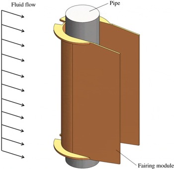
U-shaped fairing module on a 4.5 inch pipe; from Pontaza et al. (Reference Pontaza, Kotikanyadanam, Moeleker, Menon and Bhat2012).

A U-shaped fairing with an open back, shown in figure 1, is a commercial design used for suppressing riser VIVs. Pontaza & Menon (Reference Pontaza and Menon2008) numerically investigated the hydrodynamic performance of this fairing design and found that it experiences a low drag coefficient (
 $C_{d}=0.52$
at
 $\mathit{Re}\approx 10^{6}$
). The splitter plates prevent the near-wake interaction of the opposite-sign vorticity shear layers emanating from the sides of the fairing module. Therefore, flow unsteadiness in the near wake of the riser is weakened. They also recorded small-amplitude drag and lift force coefficients, which may imply that this configuration is effective. However, in Pontaza & Menon (Reference Pontaza and Menon2008) a stationary design was studied, presumably due to the complexity associated with the simulation of free VIV motion of the fairing–cylinder system.
Yu et al. (Reference Yu, Xie, Yan, Constantinides, Oakley and Karniadakis2015) performed numerical simulations of the freely vibrating fairing–cylinder system with the spectral element solver NEKTAR (Karniadakis & Sherwin Reference Karniadakis and Sherwin2013), mostly in two dimensions, hence neglecting the gaps between adjacent fairing modules. They employed a partitioned fluid–structure interaction (FSI) method (Baek & Karniadakis Reference Baek and Karniadakis2012), which led to reasonable computational scalability and efficiency. Since the rotational friction plays an important role in suppressing VIVs and reducing the drag force (Assi et al. Reference Assi, Bearman and Kitney2009), a free-to-rotate fairing model was adopted in their simulations. They found that VIV is, indeed, drastically reduced at low Reynolds numbers and the role of the friction coefficient between the fairing and cylinder was explained and quantified. Owing to the low rotational inertia of the fairing, the added-mass effect (Causin, Gerbeau & Nobile Reference Causin, Gerbeau and Nobile2005) is very strong and can severely affect the flow–structure interaction. To this end, a new method of fictitious mass (Baek & Karniadakis Reference Baek and Karniadakis2012; Yu, Baek & Karniadakis Reference Yu, Baek and Karniadakis2013) was employed, where additional acceleration terms are introduced in the structure solver to balance the added-mass effect caused by low rotational inertia, and provide stabilization when problems with large fairing rotations arise. Yu et al. (Reference Yu, Xie, Yan, Constantinides, Oakley and Karniadakis2015) also performed a three-dimensional (3D) study, where fairings of finite length are placed along the cylinder span. The fairings were homogeneous, fitted along the cylinder without gaps. However, in industrial applications, fairings of length 3–5 diameters are fitted along the riser and there always exists a gap between adjacent fairing modules.
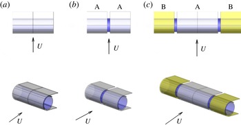
In the present study, we will extend the previous work by Yu et al. (Reference Yu, Xie, Yan, Constantinides, Oakley and Karniadakis2015) to higher Reynolds numbers and, in particular, we will investigate the effect of the gap between adjacent fairings. Three different 3D geometric models for the fairing–cylinder system are adopted, as shown in figure 2. In all configurations, periodic boundary conditions are imposed on both ends of the model in the spanwise direction, hence simulating very long fairing–cylinder systems. First, a homogeneous fairing–cylinder system is considered, which is an extension of the two-dimensional (2D) geometry along the spanwise direction. The second is a type A system with a gap (denoted by
 $G$
in the paper) following the actual fairing module used in Chevron’s experimental set-up. The third is a fairing–cylinder system of type AB with gaps between adjacent fairings. For the type A system, the grey part represents the fairing, while the blue part represents the cylinder. For the type AB configuration, the yellow part represents the second adjacent fairing. As we will show, a gap between adjacent fairings can dramatically alter the wake pattern, leading to significant drag reduction and VIV suppression and possibly to total VIV elimination. This is linked to a fundamental change in the vorticity production and redistribution around the fairing–cylinder system that we investigate in the current work.
Geometry of fairing configurations considered in this work. (a) Homogeneous fairing–cylinder system. (b) Fairing–cylinder system of type A. (c) Fairing–cylinder system of type AB.

The paper is organized as follows. In § 2, the physical model and numerical method are presented. Then, the equations of motion for the fairing–cylinder systems of type A and type AB are presented in § 3. Simulation results for the free motion of a homogeneous fairing–cylinder system at high Reynolds number are presented in § 4. Comparison of two- and 3D simulation results of homogeneous fairing–cylinder systems for various friction coefficients at
 $\mathit{Re}=1000$
are shown in § 4.1. We also provide numerical results of vibrating fairings at
 $\mathit{Re}=10\,000$
in § 4.2. Since the gap between fairings along the cylinder span affects the drag force and VIV motions, we conduct systematic numerical simulations and present the corresponding results in § 5. First, the flow around the periodic type A system at different gap distances is simulated at
 $\mathit{Re}=100$
in § 5.1. Then, the vibration behaviour of fairings with gap
 $G=0.5D$
is investigated at three different
 $\mathit{Re}$
(
 $\mathit{Re}=100$
,
 $500$
and
 $1000$
) in § 5.2. Finally, the VIVs of type AB systems are studied at
 $\mathit{Re}=100$
and
 $500$
in § 5.3. We summarize the main points of our paper in § 6.
2. Problem definition and simulation set-up
In a previous study (Yu et al.
Reference Yu, Xie, Yan, Constantinides, Oakley and Karniadakis2015), direct numerical simulations were mostly focused on 2D and low-
 $\mathit{Re}$
(
 $100\leqslant \mathit{Re}\leqslant 1000$
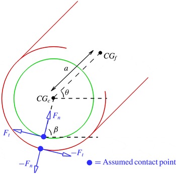
) flow for a 2D fairing–cylinder system, as shown in figure 3. The cylinder is free to respond in both the cross-flow and streamwise directions. The fairing moves following the cylinder, but with an additional degree of freedom because it can rotate around the cylinder axis, subjected to hydrodynamic torque. Owing to the gap and the three-dimensionality of the geometry, the equations for the fairing and cylinder motions are different and are presented in § 3. In the fairing–cylinder system of type A, the effect of gap is introduced by the length ratio
 $L_{f}/L_{c}$
, where
 $L_{f}$
is the spanwise length of the fairing and
 $L_{c}$
is the spanwise length of the cylinder; we have
 $L_{c}=L_{f}+G$
. Hence, if there is no gap between the fairings, with
 $G=0$
, we obtain the structure equations for a homogeneous fairing–cylinder system. In the fairing–cylinder system of type AB, there are eight equations of motion. The relationship between cylinder length and fairing length is
 $L_{c}=L_{f}+L_{g}+2G$
, where
 $L_{g}$
is the spanwise length of the second fairing.
Coordinate system and symbol definition for the fairing and cylinder motions. Here we use green to represent the cylinder and red to represent the fairing, while the contact forces are marked by blue.

For the fluid part, the flow is simulated in several 3D domains: a small domain
 $[-5,20]\times [-5,5]\times [0,L_{c}]$
with the origin
 $(0,0,0)$
located at the centre of the cylinder for
 $\mathit{Re}\leqslant 1000$
; for higher Reynolds number, a bigger and finer mesh is employed as discussed in § 4.2. The effect of blockage as well as the sensitivity to the spectral element polynomial order have been quantified in figures 5, 10 and 15 of Yu et al. (Reference Yu, Xie, Yan, Constantinides, Oakley and Karniadakis2015); it was also re-examined in the current 3D simulations. A solid cylinder with diameter
 $D_{c}=1$
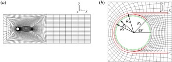
is placed at the origin with a fairing surrounding it. For the fluid solver we used a mesh consisting of hexahedral elements, built by extrusion of a 2D mesh shown in figure 4. The boundary conditions are as follows: at the inlet, a uniform steady flow with
 $U=1$
is imposed; while at the outlet, we employ a zero Neumann boundary condition. Along the cross-flow and spanwise directions, a periodic boundary condition is applied. The fairing is composed of two parts: (1) the circular body part, which covers three-quarters of the cylinder and is centred at the cylinder centre with radius
 $0.6$
; and (2) a pair of parallel plates attached to the top and bottom points of the circular part of the fairing (see the red part in figure 3). Unlike the configuration used in 2D simulations, the thickness of the plates in the fairing geometry is non-zero here. Figure 4(b) provides the detailed configuration of the fairing. The parameters in the plot are
 $R_{2}=0.55$
,
 $R_{3}=0.56$
and
 $R_{4}=0.6$
. In the undisturbed configuration, the plates are parallel to the streamwise direction, with a length of
 $1.0$
, i.e. equal to one cylinder diameter
 $D$
. The fairing’s centre of gravity is located at
 $(0.085,0)$
in the
 $(x,y)$
plane.
Fluid mesh around the fairing–cylinder system. (a) Spectral element mesh for the fluid solver. Domain size:
 $[-5,20]\times [-5,5]\times [0,L_{c}]$
, where
 $L_{c}$
is the length of the cylinder along its axis. The origin (
 $0,0,0$
) is located at the centre of the cylinder and the diameter of the cylinder is
 $D_{c}=1$
. (b) Details of mesh near the fairing–cylinder system. Here we use green to represent the cylinder and red to represent the fairing.

A fictitious inertia method is employed to stabilize the fluid–structure interaction simulations for fairings with low inertia in order to solve the coupled Navier–Stokes and structural equations (Baek & Karniadakis Reference Baek and Karniadakis2012). For the fluid model, we employ the incompressible Navier–Stokes equation expressed in an arbitrary Lagrangian–Eulerian framework (Hughes, Liu & Zimmermann Reference Hughes, Liu and Zimmermann1981). For the solid model, we discretize the structure system in time using the Newmark scheme, and apply an additional inertial term following the fictitious inertia method. Specifically, unlike in the simulations of Baek & Karniadakis (Reference Baek and Karniadakis2011), here we only needed to stabilize the rotational motion, and not the translational motion; hence, we employed only a fictitious inertia term. According to numerical tests conducted in Yu et al. (Reference Yu, Xie, Yan, Constantinides, Oakley and Karniadakis2015), the effective fictitious inertia coefficient
 $f_{I}$
takes values around
 $2.0$
and is only weakly dependent on
 $\mathit{Re}$
. Here we employ spectral elements of order
 $p=3$
and
 $p=5$
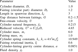
in all simulations. Simulations were performed using the physical and numerical parameters in table 1, unless stated otherwise.
All parameters are non-dimensionalized based on the cylinder diameter
 $D_{c}$
, free-stream velocity
 $U$
and fairing mass
 $m_{f}$
. The mass ratio between cylinder and fairing is
 $m_{c}/m_{f}=6$
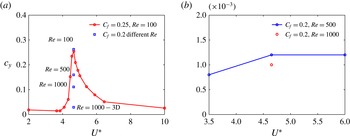
, matching the value used in the experiments conducted by Chevron. Moreover, for this mass ratio, the largest amplitude of oscillation is found around
 $U^{\ast }=4.65$
for the homogeneous fairing system at
 $\mathit{Re}=100$
. The response at the same
 $U^{\ast }$
value decreases for higher
 $\mathit{Re}$
– see figure 5(a). For the type A system, in addition to
 $U^{\ast }=4.65$
, we also investigated the response at reduced velocities 3.5 and 6 at
 $\mathit{Re}=500$
. From figure 5(b), it is seen that the VIV response is virtually eliminated for all values of
 $U^{\ast }$
. This is the reason we focus our simulations on
 $U^{\ast }=4.65$
.
VIV response
 $c_{y}$
for (a) the homogeneous fairing–cylinder system, and (b) the type A system, as a function of reduced velocity
 $U^{\ast }$
.

Non-dimensional parameters used in the numerical simulations based on the cylinder diameter
 $D_{c}$
, free-stream velocity
 $U$
and fairing mass
 $m_{f}$
.

3. Cylinder and fairing models: governing equations
3.1. Fairing–cylinder system of type A
First, we introduce the structure equations for the 3D fairing–cylinder system of type A. The cylinder is subjected to VIVs with two degrees of freedom (DOF) in the
 $(x,y)$
plane. In each
 $(x,y)$
section, the fairing and the cylinder are concentric, while the fairing is in contact with the cylinder and is free to rotate. There is a small gap between the fairing and cylinder with a single point of contact, where the fairing is pressed against the cylinder; the contact angle
 ${\it\beta}$
denotes the position of the contact point. As shown in figure 3, for each
 $(x,y)$
section the system allows body motions with five DOF, including the cylinder’s horizontal and vertical motions (
 $c_{x}$
and
 $c_{y}$
), and the fairing’s horizontal and vertical motions (
 $f_{x}$
and
 $f_{y}$
) and rotational angle (
 ${\it\theta}$
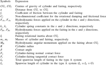
). Here we define some symbols to be used in the equations of motion; see table 2. To derive the equations of motion for the fairing–cylinder system of type A, we make the following assumptions.
-
(1) There is no damping force acting on the structure in the translational and rotational directions.
-
(2) The cylinder and the fairing are always in contact at a single point in the
 $(x,y)$
plane.
-
(3) The tangential contact force
$F_{t}$
between the cylinder and the fairing in the
$(x,y)$
plane is uniform. It is related to the normal contact force
$F_{n}$
following
$F_{t}=f_{c}F_{n}$
, where
$f_{c}$
is proportional to the sign function of
$\partial {\it\theta}/\partial t$
, with a constant sliding friction coefficient
$C_{f}$
, i.e. (3.1)Here
$$\begin{eqnarray}f_{c}=C_{f}\,\text{sgn}\left(\frac{\text{d}{\it\theta}}{\text{d}t}\right).\end{eqnarray}$$
$C_{f}$
can be seen as a measure of the rotational damping and frictional force. More details are provided in the appendix of Yu et al. (Reference Yu, Xie, Yan, Constantinides, Oakley and Karniadakis2015).


Symbols used in the type A system; see geometries in figure 2(a,b).

Based on these assumptions, the equations of motion for the cylinder are written about
 $CG_{c}$
as
 $$\begin{eqnarray}\left.\begin{array}{@{}c@{}}m_{c}{\displaystyle \frac{\partial ^{2}c_{x}}{\partial t^{2}}}L_{c}+k_{x}c_{x}L_{c}-F_{n}(\cos {\it\beta}+f_{c}\sin {\it\beta})L_{f}=F_{chx},\\ m_{c}{\displaystyle \frac{\partial ^{2}c_{y}}{\partial t^{2}}}L_{c}+k_{y}c_{y}L_{c}-F_{n}(\sin {\it\beta}-f_{c}\cos {\it\beta})L_{f}=F_{chy},\end{array}\right\}\end{eqnarray}$$
and the equations of motion for the fairing are written about
 $CG_{f}$
as
 $$\begin{eqnarray}\left.\begin{array}{@{}c@{}}\displaystyle m_{f}{\displaystyle \frac{\partial ^{2}f_{x}}{\partial t^{2}}}L_{f}+F_{n}(\cos {\it\beta}+f_{c}\sin {\it\beta})L_{f}=F_{fhx},\\ \displaystyle m_{f}{\displaystyle \frac{\partial ^{2}f_{y}}{\partial t^{2}}}L_{f}+F_{n}(\sin {\it\beta}-f_{c}\cos {\it\beta})L_{f}=F_{fhy}.\end{array}\right\}\end{eqnarray}$$
From figure 3, we can see that the centres of gravity of the cylinder and fairing are geometrically related as
 $$\begin{eqnarray}c_{x}=f_{x}-a\cos {\it\theta},\quad c_{y}=f_{y}-a\sin {\it\theta}.\end{eqnarray}$$
Substituting these expressions into (3.2), the equations of motion for the cylinder become
 $$\begin{eqnarray}\displaystyle & & \displaystyle m_{c}\left[{\displaystyle \frac{\partial ^{2}f_{x}}{\partial t^{2}}}+a\left(\left({\displaystyle \frac{\partial {\it\theta}}{\partial t}}\right)^{2}\cos {\it\theta}+{\displaystyle \frac{\partial ^{2}{\it\theta}}{\partial t^{2}}}\sin {\it\theta}\right)\right]L_{c}\nonumber\\ \displaystyle & & \displaystyle \quad +\,k_{x}[f_{x}-a\cos {\it\theta}]L_{c}-F_{n}(\cos {\it\beta}+f_{c}\sin {\it\beta})L_{f}=F_{chx},\end{eqnarray}$$
 $$\begin{eqnarray}\displaystyle & & \displaystyle m_{c}\left[{\displaystyle \frac{\partial ^{2}f_{y}}{\partial t^{2}}}+a\left(\left({\displaystyle \frac{\partial {\it\theta}}{\partial t}}\right)^{2}\sin {\it\theta}-{\displaystyle \frac{\partial ^{2}{\it\theta}}{\partial t^{2}}}\cos {\it\theta}\right)\right]L_{c}\nonumber\\ \displaystyle & & \displaystyle \quad +\,k_{y}[f_{y}-a\sin {\it\theta}]L_{c}-F_{n}(\sin {\it\beta}-f_{c}\cos {\it\beta})L_{f}=F_{chy}.\end{eqnarray}$$
In addition, we can derive an equation for the angular momentum. The total angular momentum
 $I_{f}\ddot{{\it\theta}}$
about
 $CG_{f}$
should be equal to the resultant angular momentum exerted by the fairing–cylinder contact force and the hydrodynamic angular momentum
 $M_{fh}$
from the fluid. Specifically, the torque of the fairing–cylinder normal contact force
 $F_{n}$
about
 $CG_{f}$
is
 $a\sin ({\it\beta}-{\it\theta})$
, and the torque of the fairing–cylinder tangential contact force
 $F_{t}$
is
 $-(a\cos ({\it\beta}-{\it\theta})+R)$
. Therefore, we have the resultant angular momentum as
 $$\begin{eqnarray}M_{fh}+F_{n}a\sin ({\it\beta}-{\it\theta})L_{f}-F_{t}(a\cos ({\it\beta}-{\it\theta})+R)L_{f}.\end{eqnarray}$$
By substituting the relation
 $F_{t}=f_{c}F_{n}$
, the conservation of angular momentum can be expressed as
 $$\begin{eqnarray}I_{f}{\displaystyle \frac{\partial ^{2}{\it\theta}}{\partial t^{2}}}L_{f}-F_{n}[a\sin ({\it\beta}-{\it\theta})-af_{c}\cos ({\it\beta}-{\it\theta})-Rf_{c}]L_{f}=M_{fh}.\end{eqnarray}$$
Combining the equations of motion for the fairing (3.3) and the equations for the cylinder (3.5), we obtain a system with five equations consisting of five unknowns
 $(f_{x},f_{y},{\it\theta},{\it\beta},F_{n})$
:
 $$\begin{eqnarray}\displaystyle & & \displaystyle m_{c}\left[{\displaystyle \frac{\partial ^{2}f_{x}}{\partial t^{2}}}+a\left(\left({\displaystyle \frac{\partial {\it\theta}}{\partial t}}\right)^{2}\cos {\it\theta}+{\displaystyle \frac{\partial ^{2}{\it\theta}}{\partial t^{2}}}\sin {\it\theta}\right)\right]L_{c}\nonumber\\ \displaystyle & & \displaystyle \quad +\,k_{x}[f_{x}-a\cos {\it\theta}]L_{c}-F_{n}(\cos {\it\beta}+f_{c}\sin {\it\beta})L_{f}=F_{chx},\end{eqnarray}$$
 $$\begin{eqnarray}\displaystyle & & \displaystyle m_{c}\left[{\displaystyle \frac{\partial ^{2}f_{y}}{\partial t^{2}}}+a\left(\left({\displaystyle \frac{\partial {\it\theta}}{\partial t}}\right)^{2}\sin {\it\theta}-{\displaystyle \frac{\partial ^{2}{\it\theta}}{\partial t^{2}}}\cos {\it\theta}\right)\right]L_{c}\nonumber\\ \displaystyle & & \displaystyle \quad +\,k_{y}[f_{y}-a\sin {\it\theta}]L_{c}-F_{n}(\sin {\it\beta}-f_{c}\cos {\it\beta})L_{f}=F_{chy}.\end{eqnarray}$$
 $$\begin{eqnarray}\displaystyle & & \displaystyle m_{f}{\displaystyle \frac{\partial ^{2}f_{x}}{\partial t^{2}}}L_{f}+F_{n}(\cos {\it\beta}+f_{c}\sin {\it\beta})L_{f}=F_{fhx},\end{eqnarray}$$
 $$\begin{eqnarray}\displaystyle & & \displaystyle m_{f}{\displaystyle \frac{\partial ^{2}f_{y}}{\partial t^{2}}}L_{f}+F_{n}(\sin {\it\beta}-f_{c}\cos {\it\beta})L_{f}=F_{fhy}\end{eqnarray}$$
 $$\begin{eqnarray}\displaystyle & & \displaystyle I_{f}{\displaystyle \frac{\partial ^{2}{\it\theta}}{\partial t^{2}}}L_{f}-F_{n}[a\sin ({\it\beta}-{\it\theta})-af_{c}\cos ({\it\beta}-{\it\theta})-R_{c}f_{c}]L_{f}=M_{fh}.\end{eqnarray}$$
3.2. Fairing–cylinder system of type AB
In the type AB system, there are two different fairings interacting with the cylinder within the computational domain. Just as in the type A system, the set-up of the second fairing is the same as that of the first fairing, except that it is located between two other fairings at the ends (which, due to periodicity, are effectively part of the same fairing). The type AB system allows motions with eight DOF, including the cylinder’s horizontal and vertical motions (
 $c_{x}$
and
 $c_{y}$
), the first fairing’s horizontal and vertical motions (
 $f_{x}$
and
 $f_{y}$
) and rotational angle (
 ${\it\theta}$
), and the second fairing’s horizontal and vertical motions (
 $g_{x}$
and
 $g_{y}$
) and rotational angle (
 ${\it\zeta}$
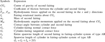
). Here we define the symbols to be used in the equations of motion for the fairings in table 3. To derive the equations of motions for the fairing–cylinder system of type AB, we employ two additional assumptions.
-
(a) The cylinder and the two fairings are always in contact at a single point in the
$(x,y)$
plane for each fairing. -
(b) The tangential contact force
$G_{t}$
between the cylinder and the second fairing in the
$(x,y)$
plane is uniform. It is related to the normal contact force
$G_{n}$
following
$G_{t}=f_{g}G_{n}$
, where
$f_{g}$
is proportional to the sign function of
$\partial {\it\zeta}/\partial t$
with a constant sliding friction coefficient
$C_{g}$
, i.e.(3.9)Here
$$\begin{eqnarray}f_{g}=C_{g}\,\text{sgn}\left(\frac{\text{d}{\it\zeta}}{\text{d}t}\right).\end{eqnarray}$$
$C_{g}$
represents a measure of the rotational damping and frictional force for the second fairing.


Symbols used in the type AB system – see geometry in figure 2(c).

Based on these assumptions, the equations of motion for the cylinder are written about the
 $CG_{c}$
as
 $$\begin{eqnarray}\left.\begin{array}{@{}c@{}}\displaystyle m_{c}{\displaystyle \frac{\partial ^{2}c_{x}}{\partial t^{2}}}L_{c}+k_{x}c_{x}L_{c}-F_{n}(\cos {\it\beta}+f_{c}\sin {\it\beta})L_{f}-G_{n}(\cos {\it\alpha}+f_{g}\sin {\it\alpha})L_{g}=F_{chx},\\ \displaystyle m_{c}{\displaystyle \frac{\partial ^{2}c_{y}}{\partial t^{2}}}L_{c}+k_{y}c_{y}L_{c}-F_{n}(\sin {\it\beta}-f_{c}\cos {\it\beta})L_{f}-G_{n}(\sin {\it\alpha}-f_{g}\cos {\it\alpha})L_{g}=F_{chy},\end{array}\right\}\end{eqnarray}$$
the equations of motion for the first fairing are written about the
 $CG_{f}$
in the same way as in (3.3), and the equations of motion for the second fairing are written about
 $CG_{g}$
in a similar way to (3.3) as
 $$\begin{eqnarray}\left.\begin{array}{@{}c@{}}m_{g}{\displaystyle \frac{\partial ^{2}g_{x}}{\partial t^{2}}}L_{g}+G_{n}(\cos {\it\beta}+f_{g}\sin {\it\beta})L_{g}=F_{ghx},\\ m_{g}{\displaystyle \frac{\partial ^{2}g_{y}}{\partial t^{2}}}L_{g}+G_{n}(\sin {\it\beta}-f_{g}\cos {\it\beta})L_{g}=F_{ghy}.\end{array}\right\}\end{eqnarray}$$
Since there are two different fairings rotating and interacting around the cylinder, we can see that the centres of gravity of the cylinder and the two fairings are geometrically related as
 $$\begin{eqnarray}\left.\begin{array}{@{}c@{}}\displaystyle f_{x}=c_{x}+a\cos {\it\theta},\quad f_{y}=c_{y}+a\sin {\it\theta},\\ \displaystyle g_{x}=c_{x}+a\cos {\it\zeta},\quad g_{y}=c_{y}+a\sin {\it\zeta}.\end{array}\right\}\end{eqnarray}$$
Substituting these expressions into (3.11) and (3.3), the equations of motion for the fairing–cylinder system of type AB become
 $$\begin{eqnarray}\left.\begin{array}{@{}c@{}}\displaystyle m_{f}\left[{\displaystyle \frac{\partial ^{2}c_{x}}{\partial t^{2}}}-a\left(\left({\displaystyle \frac{\partial {\it\theta}}{\partial t}}\right)^{2}\sin {\it\theta}+{\displaystyle \frac{\partial ^{2}{\it\theta}}{\partial t^{2}}}\cos {\it\theta}\right)\right]L_{f}+F_{n}(\cos {\it\beta}+f_{c}\sin {\it\beta})L_{f}=F_{fhx},\\ \displaystyle m_{f}\left[{\displaystyle \frac{\partial ^{2}c_{y}}{\partial t^{2}}}+a\left(\left({\displaystyle \frac{\partial {\it\theta}}{\partial t}}\right)^{2}\cos {\it\theta}-{\displaystyle \frac{\partial ^{2}{\it\theta}}{\partial t^{2}}}\sin {\it\theta}\right)\right]L_{f}+F_{n}(\sin {\it\beta}-f_{c}\cos {\it\beta})L_{f}=F_{fhy},\\ \displaystyle m_{g}\left[{\displaystyle \frac{\partial ^{2}c_{x}}{\partial t^{2}}}-a\left(\left({\displaystyle \frac{\partial {\it\zeta}}{\partial t}}\right)^{2}\sin {\it\zeta}+{\displaystyle \frac{\partial ^{2}{\it\zeta}}{\partial t^{2}}}\cos {\it\zeta}\right)\right]L_{g}+G_{n}(\cos {\it\alpha}+f_{g}\sin {\it\alpha})L_{g}=F_{ghx},\\ \displaystyle m_{g}\left[{\displaystyle \frac{\partial ^{2}c_{y}}{\partial t^{2}}}+a\left(\left({\displaystyle \frac{\partial {\it\zeta}}{\partial t}}\right)^{2}\cos {\it\zeta}-{\displaystyle \frac{\partial ^{2}{\it\zeta}}{\partial t^{2}}}\sin {\it\zeta}\right)\right]L_{g}+G_{n}(\sin {\it\alpha}-f_{g}\cos {\it\alpha})L_{g}=F_{ghy}.\end{array}\right\}\end{eqnarray}$$
In addition, we can derive another equation from the conservation of angular momentum for the second fairing, which is the same as the first fairing in (3.7):
 $$\begin{eqnarray}I_{g}{\displaystyle \frac{\partial ^{2}{\it\zeta}}{\partial t^{2}}}L_{g}-G_{n}[a\sin ({\it\alpha}-{\it\zeta})-af_{g}\cos ({\it\alpha}-{\it\zeta})-R_{c}f_{g}]L_{g}=M_{gh}.\end{eqnarray}$$
With the type AB system, we can obtain a system of eight equations in eight unknowns,
 $(c_{x},c_{y},{\it\theta},{\it\beta},F_{n},{\it\zeta},{\it\alpha},G_{n})$
:
 $$\begin{eqnarray}\left.\begin{array}{@{}c@{}}\displaystyle m_{c}{\displaystyle \frac{\partial ^{2}c_{x}}{\partial t^{2}}}L_{c}+k_{x}c_{x}L_{c}-F_{n}(\cos {\it\beta}+f_{c}\sin {\it\beta})L_{f}-G_{n}(\cos {\it\alpha}+f_{g}\sin {\it\alpha})L_{g}=F_{chx},\\ \displaystyle m_{c}{\displaystyle \frac{\partial ^{2}c_{y}}{\partial t^{2}}}L_{c}+k_{y}c_{y}L_{c}-F_{n}(\sin {\it\beta}-f_{c}\cos {\it\beta})L_{f}-G_{n}(\sin {\it\alpha}-f_{g}\cos {\it\alpha})L_{g}=F_{chy},\\ \displaystyle m_{f}\left[{\displaystyle \frac{\partial ^{2}c_{x}}{\partial t^{2}}}-a\left(\left({\displaystyle \frac{\partial {\it\theta}}{\partial t}}\right)^{2}\sin {\it\theta}+{\displaystyle \frac{\partial ^{2}{\it\theta}}{\partial t^{2}}}\cos {\it\theta}\right)\right]L_{f}+F_{n}(\cos {\it\beta}+f_{c}\sin {\it\beta})L_{f}=F_{fhx},\\ \displaystyle m_{f}\left[{\displaystyle \frac{\partial ^{2}c_{y}}{\partial t^{2}}}+a\left(\left({\displaystyle \frac{\partial {\it\theta}}{\partial t}}\right)^{2}\cos {\it\theta}-{\displaystyle \frac{\partial ^{2}{\it\theta}}{\partial t^{2}}}\sin {\it\theta}\right)\right]L_{f}+F_{n}(\sin {\it\beta}-f_{c}\cos {\it\beta})L_{f}=F_{fhy},\\ \displaystyle m_{g}\left[{\displaystyle \frac{\partial ^{2}c_{x}}{\partial t^{2}}}-a\left(\left({\displaystyle \frac{\partial {\it\zeta}}{\partial t}}\right)^{2}\sin {\it\zeta}+{\displaystyle \frac{\partial ^{2}{\it\zeta}}{\partial t^{2}}}\cos {\it\zeta}\right)\right]L_{g}+G_{n}(\cos {\it\alpha}+f_{g}\sin {\it\alpha})L_{g}=F_{ghx},\\ \displaystyle m_{f}\left[{\displaystyle \frac{\partial ^{2}c_{y}}{\partial t^{2}}}+a\left(\left({\displaystyle \frac{\partial {\it\zeta}}{\partial t}}\right)^{2}\cos {\it\zeta}-{\displaystyle \frac{\partial ^{2}{\it\zeta}}{\partial t^{2}}}\sin {\it\zeta}\right)\right]L_{g}+G_{n}(\sin {\it\alpha}-f_{g}\cos {\it\alpha})L_{g}=F_{ghy},\\ \displaystyle I_{f}{\displaystyle \frac{\partial ^{2}{\it\theta}}{\partial t^{2}}}L_{f}-F_{n}[a\sin ({\it\beta}-{\it\theta})-af_{c}\cos ({\it\beta}-{\it\theta})-Rf_{c}]L_{f}=M_{fh},\\ \displaystyle I_{g}{\displaystyle \frac{\partial ^{2}{\it\zeta}}{\partial t^{2}}}L_{g}-G_{n}[a\sin ({\it\alpha}-{\it\zeta})-af_{g}\cos ({\it\alpha}-{\it\zeta})-Rf_{g}]L_{g}=M_{gh}.\end{array}\right\}\end{eqnarray}$$
4. Vortex-induced vibrations of homogeneous fairing system
By conducting simulations with varying initial perturbations, we found that the flow around the fairing is 3D at
 $\mathit{Re}=1000$
. To perform 3D simulations, we extrude the fairing model in two dimensions along the spanwise direction by a length
 $L=\text{3D}$
, where
 $D$
is the cylinder diameter. Typically, in applications the spanwise length of the U-shaped fairing configuration is in the range of 3D–5D (Pontaza & Menon Reference Pontaza and Menon2008). Here we use the value at the lower end of the range to reduce computational cost. We consider first the flow transition to three-dimensionality and its effects on the vibration of the fairing (see § 4.1) at
 $\mathit{Re}=1000$
. We also perform large-eddy simulations (LES) at a higher Reynolds number,
 $\mathit{Re}=10\,000$
, in § 4.2. To this end, we will employ a new LES model we implemented recently in NEKTAR based on the variational multiscale large-eddy simulation (VMLES) model (Luo et al.
Reference Luo, Epps, Chryssostomidis and Karniadakis2011).
We define the drag and lift coefficients as
 $$\begin{eqnarray}\displaystyle & \displaystyle C_{d}=\frac{F_{d}}{0.5{\it\rho}U^{2}DL}, & \displaystyle\end{eqnarray}$$
 $$\begin{eqnarray}\displaystyle & \displaystyle C_{l}=\frac{F_{l}}{0.5{\it\rho}U^{2}DL}, & \displaystyle\end{eqnarray}$$
 $F_{d}$
and
 $F_{l}$
are the drag and lift forces, respectively. These are denoted separately as
 $F_{chx}$
and
 $F_{chy}$
for the cylinder, and
 $F_{fhx}$
and
 $F_{fhy}$
for the fairing. For the fairing, the diameter is
 $D_{f}=1.2$
and the spanwise length is
 $L_{f}=\text{3D}$
for all simulations. For the cylinder, the diameter is
 $D_{c}=1$
and the spanwise length depends on the gap
 $G$
, which is
 $L_{c}=L_{f}+G$
for the homogeneous fairing–cylinder system and for the fairing–cylinder system of type A, and
 $L_{c}=L_{f}+L_{g}+2G$
for the fairing–cylinder system of type AB.
4.1. Effect of three-dimensionality
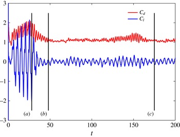
First, we simulated the 3D flow around a stationary fairing to obtain the initial conditions for the flow field for the moving fairing simulations. Figure 6 shows the time traces of the drag and lift coefficients of the fairing, which have been used in Yu et al. (Reference Yu, Xie, Yan, Constantinides, Oakley and Karniadakis2015). After time
 $t\geqslant 34$
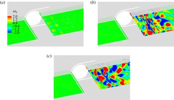
, both the drag and lift coefficients drop quickly and exhibit a non-periodic behaviour, marking the transition from 2D flow to 3D flow. The fairing experiences significantly lower drag and lift forces in 3D flow compared to 2D flow. Instantaneous vorticity contours in the cross-flow direction (
 ${\it\omega}_{y}$
) are used to represent the transition from two- to three-dimensionality. In figure 7 we present three different snapshots of
 ${\it\omega}_{y}$
contours, at (a)
 $t=28~\text{s}$
, (b)
 $t=48~\text{s}$
and (c)
 $t=175~\text{s}$
, corresponding to flow in a 2D state, transition state and 3D fully developed state. The intensity of three-dimensionality is already high in the transition state, as shown in figure 7.
Transition to three-dimensionality (static configuration): time traces of hydrodynamic drag and lift coefficients on the fairing part for the homogeneous fairing system at
 $\mathit{Re}=1000$
.

Instantaneous vorticity contours in the cross-flow direction (
 ${\it\omega}_{y}$
) around the homogeneous fairing at the centreline plane (
 $x\in (-1.7,5.5),y=0,z\in (0,3)$
) at
 $\mathit{Re}=1000$
: (a)
 $t=28$
, (b)
 $t=48$
and (c)
 $t=175$
.

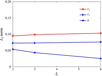
The
 $L_{2}$
norm of the vibratory responses of the homogeneous fairing system (
 $c_{x},c_{y},{\it\theta}$
) versus the rotational inertia of the homogeneous fairing,
 $I_{f}$
, for a constant friction coefficient
 $C_{f}=0.2$
at
 $\mathit{Re}=1000$
.

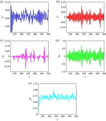
Time history of the motion of the homogeneous fairing system for 3D flow at
 $\mathit{Re}=1000$
for
 $C_{f}=0.1$
: (a)
 $x$
displacement of the cylinder,
 $c_{x}$
; (b)
 $y$
displacement of the cylinder,
 $c_{y}$
; (c) fairing rotation angle
 ${\it\theta}$
; (d) contact angle
 ${\it\beta}$
between the fairing and the cylinder at the contact point; and (e) contact force
 $F_{n}$
between the fairing and the cylinder at the contact point.

The
 $L_{2}$
norm of the vibratory responses of the homogeneous fairing system at
 $\mathit{Re}=1000$
as a function of
 $C_{f}$
: (a) streamwise displacement of the cylinder
 $c_{x}$
; (b) cross-flow displacement of the cylinder
 $c_{y}$
; (c) fairing rotation angle
 ${\it\theta}$
; and (d) contact angle
 ${\it\beta}$
.

Next, we present the results for both 2D and 3D flow around moving fairings for different values of the friction coefficient
 $C_{f}$
, ranging from 0.1 to 0.5, and compare the effect of three-dimensionality on the structural motion. The inertia of the fairing is set at
 $I_{f}=0.6$
for 3D flow, but for 2D flow a larger value is employed,
 $I_{f}=6.0$
, to prevent very large rotations and hence extreme deformation of the mesh. Figure 8 shows the effect of inertia on the structural motion for a friction coefficient
 $C_{f}=0.2$
and for 2D flow. Here, the
 $L_{2}$
norm is defined as
 $\sqrt{\sum _{k=1}^{n}|x_{k}|^{2}}$
, where
 $x_{k}$
denotes the time instant of the structure motion. Even though the rotation of the fairing decreases for larger
 $I_{f}$
, the translational motion remains nearly constant. We compare the results from these two simulations to investigate the effect of three-dimensionality: in 3D flow, the response of the fairing follows a non-periodic motion as seen in figure 9. We use the
 $L_{2}$
norm in figure 10 to plot the vibration response results (
 $c_{x},c_{y},{\it\theta},{\it\beta}$
) for 2D flow (circles) and 3D flow (triangles) at
 $\mathit{Re}=1000$
. The 2D simulations overpredict the VIVs of the structure, which is also affected by the specific value of
 $C_{f}$
. With the increase of friction coefficient
 $C_{f}$
, the
 $x$
displacement of the cylinder increases in the 2D simulations; the same behaviour is also observed for the cross-flow displacement, as well as the rotation angle of the fairing (
 ${\it\theta}$
) and the contact angle
 ${\it\beta}$
.
To achieve the maximum VIV suppression, a friction coefficient
 $C_{f}=0.1$
should be selected, according to the 2D simulations. However, in 3D flow, the
 $x$
displacement of the cylinder increases to
 $c_{x}=0.063$
at
 $C_{f}=0.2$
and then decreases to
 $c_{x}=0.061$
at
 $C_{f}=0.5$
. For the cross-flow displacement of the cylinder (
 $c_{y}$
) as well as the rotation angle of the fairing (
 ${\it\theta}$
), a similar pattern is observed. On the other hand, 3D simulation results at
 $\mathit{Re}=1000$
are more consistent with the trends of the 2D simulation results obtained at lower values of Reynolds number, i.e. at
 $\mathit{Re}=100$
and 500. The value
 $C_{f}=0.5$
is the best choice in 3D flow at
 $\mathit{Re}=1000$
for the most effective VIV suppression.
Time history of the motion of the homogeneous fairing system for two friction coefficients,
 $C_{f}=0.0$
(solid lines) and
 $C_{f}=0.1$
(dashed lines), at Reynolds number
 $\mathit{Re}=10\,000$
: (a) streamwise cylinder displacement
 $c_{x}$
; (b) cross-flow cylinder displacement
 $c_{y}$
; and (c) rotation angle
 ${\it\theta}$
of the fairing around the cylinder.

The
 $L_{2}$
norm of the response and the forces (
 $c_{x},c_{y},{\it\theta},C_{d},C_{l}$
) for the homogeneous fairing system, with friction coefficient
 $C_{f}=0.1$
, and for various Reynolds numbers.

4.2. Free motion at higher Reynolds number:
$\mathit{Re}=10\,000$

We now conduct a 3D simulation at higher
 $\mathit{Re}=10\,000$
, using a large computational domain, with the wake region extending
 $50D_{c}$
, where
 $D_{c}$
is the cylinder diameter. The free motion traces of the homogeneous fairing system at two different values of the friction coefficient
 $C_{f}$
are compared. Figure 11 shows the time traces of structural motions, which are (a) streamwise cylinder displacement
 $c_{x}$
, (b) cross-flow cylinder displacement
 $c_{y}$
and (c) fairing rotation angle
 ${\it\theta}$
. Here, the solid lines denote results for
 $C_{f}=0.0$
, while the dashed lines represent the case
 $C_{f}=0.1$
. Through FFT analysis, we find that there are two response frequencies, and they are almost the same for the two different
 $C_{f}$
. The response frequencies are close to the vortex shedding frequency of the stationary uniform fairing system at
 $\mathit{Re}=10\,000$
,
 $f_{o}=0.167$
, and the natural frequency of the cylinder, around
 $f_{N}=0.215$
, respectively. With increasing
 $C_{f}$
from 0 to 0.1, the vibration in the streamwise direction does not change noticeably, but both the cross-flow displacement of the cylinder and the fairing rotation decrease.
In figure 12 we plot the VIV amplitudes versus the Reynolds number, from
 $\mathit{Re}=100$
to
 $\mathit{Re}=10\,000$
. As the Reynolds number increases, the
 $L_{2}$
norm of the displacement in the streamwise direction,
 $c_{x}$
, decreases from 0.09 to 0.05, the root mean square of the displacement in the cross-flow direction,
 $c_{y}$
, decreases from 0.18 to 0.03, and the fairing rotation,
 ${\it\theta}$
, decreases from 0.12 to 0.025 rad. Both drag and lift coefficients also decrease with
 $\mathit{Re}$
. The results illustrate that the fairing experiences lower VIV motions at higher
 $\mathit{Re}$
. However, even at the high Reynolds number
 $\mathit{Re}=10\,000$
, the drag force coefficient of the fairing part is still around
 $C_{d}=0.9$
, which is much larger than the values
 $C_{d}=0.52$
for
 $\mathit{Re}=10^{6}$
for a static fairing in Pontaza & Menon (Reference Pontaza and Menon2008) and
 $C_{d}=0.50{-}0.55$
at
 $\mathit{Re}=(1.79{-}5.65)\times 10^{6}$
from experimental data in Corson et al. (Reference Corson, Cosgrove and Constantinides2014).
5. Effect of gap on two different fairing–cylinder systems
In this section, we investigate the effect of the spanwise gap in the Reynolds-number range
 $\mathit{Re}=100{-}1000$
. We study two different configurations: (1) the type A system and (2) the type AB system.
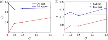
The
 $L_{2}$
norm of the force coefficients on the fairing and the cylinder of a stationary type A system at
 $\mathit{Re}=100$
, for various gap values: (a) drag coefficient
 $C_{d}$
and (b) lift coefficient
 $C_{l}$
.

Time history of the lift coefficient of the fairing and the cylinder of a stationary type A system at
 $\mathit{Re}=100$
for three different gap values: (a)
 $G=0.2D$
, (b)
 $G=0.5D$
and (c)
 $G=1.5D$
.

FFT analysis of figure 14 at
 $\mathit{Re}=100$
. (a) Frequency of lift coefficient as a function of the gap. (b) Phase difference in the lift forces of the fairing and the cylinder (stationary case).

5.1. Type A system at
$\mathit{Re}=100$

First we simulate the flow around a type A system at three different gap values,
 $G=0.2D$
,
 $0.5D$
and
 $1.5D$
. Compared to the homogeneous fairing system, a gap lowers the drag coefficient of the fairing but increases the drag coefficient of the cylinder, owing to the exposure of the surface at the gap region; see figure 13. In terms of the lift coefficient, a similar trend is observed for the cylinder. However, for the fairing, only when the gap is
 $G=0.5D$
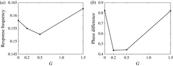
is the lift force smaller than that of the homogeneous fairing–cylinder system (which is the lowest one). Moreover, figure 14 presents the time history of the lift force coefficients for the fairing and cylinder for different gap sizes. Through FFT analysis, the response frequency of the lift coefficients is found to be the same for the cylinder and the fairing, although there is a phase difference between the two coefficients. Figure 15 presents the response frequency and phase difference versus the gap distance. For
 $G=0.2D$
or
 $0.5D$
, the response frequency is smaller than that of the homogeneous fairing–cylinder system, while for
 $G=1.5D$
the response frequency is even larger than that for the homogeneous fairing–cylinder system. We also note that the trend of the phase angle between the lift coefficient of the fairing and the cylinder is the same.
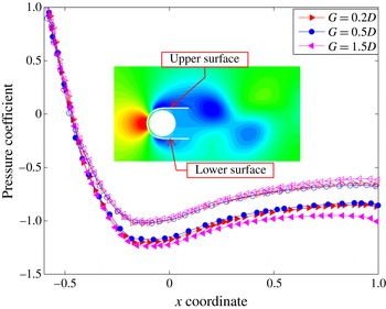
Next we consider the pressure distribution on the structure surface. Figure 16 shows instantaneous distributions of the pressure coefficient on the fairing surface at the
 $z=-0.25$
plane, where the solid symbols represent the upper surface of the fairing while the empty symbols correspond to the lower surface of the fairing. The pressure coefficient here is defined with respect to the pressure at an upstream point
 $(-5,0,-0.25)$
as
 $$\begin{eqnarray}C_{p}(x,y)=\frac{2(p(x,y,-0.25)-p(-5,0,-0.25))}{{\it\rho}_{f}U^{2}}.\end{eqnarray}$$
We can see that, for
 $G=0.5D$
, the pressure difference between the upper and lower surfaces is the smallest; this is consistent with the lowest lift force at this gap size.
Distribution of the pressure coefficient on the fairing surface of a stationary type A system for
 $\mathit{Re}=100$
, at maximum lift force. Solid symbols denote the upper surface, while empty symbols denote the lower surface.

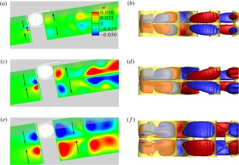
Three-dimensional flow patterns around the stationary type A system at
 $\mathit{Re}=100$
for three different gaps: (a,b)
 $G=0.2D$
, (c,d)
 $G=0.5D$
, (e,f)
 $G=1.5D$
. (a,c,e) Spanwise velocity at the centreline plane. (b,d,f) Vorticity isosurfaces: red,
 ${\it\omega}_{x}=0.1$
; blue,
 ${\it\omega}_{x}=-0.1$
; yellow,
 ${\it\omega}_{z}=\pm 0.5$
. The arrows indicate the direction of flow near the gap and in the wake. (Plots show results at maximum lift force.)

Effect of gap on the
 $L_{2}$
norm of the motion of the stationary type A system at
 $\mathit{Re}=100$
for free vibrations. Here
 $c_{x}$
and
 $c_{y}$
denote the cylinder displacements, and
 ${\it\theta}$
the fairing rotation.

Effect of gap on the
 $L_{2}$
norm force coefficients of the type A system at
 $\mathit{Re}=100$
for free vibrations: (a) cylinder part and (b) fairing part.

The gap causes the flow to become 3D even at the subcritical Reynolds number of
 $\mathit{Re}=100$
. Figure 17(a,c,e) shows the spanwise velocity contours at the centreline plane for three gap sizes. There is a strong flow interaction between the adjacent fairings in the gap region. In the plots, the arrows denote the direction of the flow near the gap and in the wake. When the gap is small, e.g.
 $G=0.2D$
and
 $0.5D$
, the flow converges at the front of the fairing in the gap region, but in the wake the flow diverges towards the opposite spanwise directions. However, when the gap is
 $G=1.5D$
, the flow converges in the wake region as well. Figure 17(b,d,f) shows isosurfaces of streamwise vorticity (red and blue) and spanwise vorticity (yellow) around the type A system. At the upstream part of the fairing, we can observe the increase of spanwise vorticity, whose intensity becomes stronger for larger gaps. In the wake of the fairing, the vorticity shows patterns resembling the mode-A instability in plain cylinder flow for
 $\mathit{Re}=220$
, with a spanwise wavelength equal to the length of the type A system. For larger gaps, the intensity of streamwise vorticity becomes stronger as well. In the far wake, the pattern of the spanwise vorticity for
 $G=1.5D$
has a horseshoe form, with the direction of the horseshoe facing downstream for
 $G=1.5D$
, and upstream for
 $G=0.2D$
and
 $0.5D$
.
In § 4.1, we found that the free motion of the fairing decreases with increasing values of
 $C_{f}$
. Here we adopt a friction coefficient of
 $C_{f}=0.2$
to simulate the free vibration and rotation of the type A system and compare with the response of the homogeneous fairing system at the same
 $C_{f}$
and
 $\mathit{Re}$
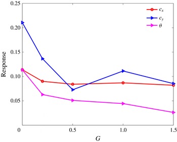
. For free motion, the response of the type A system is shown in figure 18. The gap causes the cylinder motion and fairing rotation to decrease. For the cross-flow cylinder displacement, the response varies in the range
 $0.5D\leqslant G\leqslant 1.5D$
, with the smallest value at
 $G=0.5D$
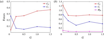
. The force coefficients for the fairing and the cylinder are also shown in figure 19. For the drag coefficient, the trend is similar to that in the stationary configuration, i.e.
 $C_{d}$
increases with
 $G$
for the cylinder and decreases for the fairing. In contrast, the lift coefficients and angular momentum of the fairing are smaller at larger gaps. Specifically, owing to the smallest cross-flow vibration, the fairing experiences the lowest lift coefficient for a gap
 $G=0.5D$
.
In summary, the presence of the gap between adjacent fairings can help suppress VIVs and also reduce the drag force even at low
 $\mathit{Re}=100$
, with the gap distance
 $G=0.5D$
being the most effective choice from all the cases we investigated.
5.2. Effect of Reynolds number on fairing–cylinder system of type A
The study so far has been conducted at low
 $\mathit{Re}$
to avoid lengthy simulations, but we will investigate next the effect of the gap at two higher Reynolds numbers,
 $\mathit{Re}=500$
and
 $1000$
, at the specific gap value of
 $G=0.5D$
. First, we compare the results with the homogeneous fairing system and the plain cylinder, shown in figure 20 for the stationary cases. With increasing
 $\mathit{Re}$
, the drag coefficient
 $C_{d}$
decreases. The fairing geometry, however, can help reduce the drag force coefficient. The homogeneous fairing system reduces the drag coefficient
 $C_{d}$
by
 $15\,\%$
, compared to the plain cylinder case, and the fairing with gap (
 $G=0.5D$
) can substantially reduce further, by almost
 $50\,\%$
, the
 $C_{d}$
at higher
 $\mathit{Re}$
. This is due to the faster pressure recovery in the open region in the wake between the parallel plates of the fairing; see figure 21. By comparing
 $z$
slices at
 $z=0.75$
, we can see that vortices are shed much farther from the tip of the fairing at
 $\mathit{Re}=500$
and
 $\mathit{Re}=1000$
, at a position of about
 $L=\text{3D}$
and
 $L=\text{4D}$
away from the cylinder centre, respectively. The flow in the wake is no longer symmetric along the spanwise direction at high
 $\mathit{Re}$
, as seen in figure 21(c,e); in fact, the wake becomes incoherent, as shown in figure 21(d,f).
We further investigate the VIVs when free motion is allowed for a gap
 $G=0.5$
and friction coefficient
 $C_{f}=0.2$
, and compare the resulting motions with those at lower
 $\mathit{Re}=100$
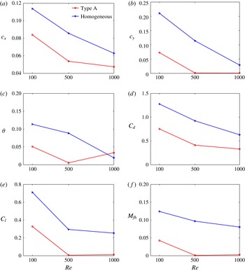
(see figure 22). These results confirm that the gap geometry suppresses VIVs at high
 $\mathit{Re}$
, but even more effectively than at lower
 $\mathit{Re}$
. As the Reynolds number increases, the difference in the streamwise vibration of the homogeneous and type A configurations decreases as a function of the gap. In contrast, the cross-flow vibration of the type A system drops quickly; e.g. at
 $\mathit{Re}=500$
the value decreases to
 $c_{y}=0.01$
. The rotation of the fairing also decreases for the type A system at
 $\mathit{Re}=100$
and
 $500$
. In terms of the force coefficients, as compared to the homogeneous fairing, the gap in the type A system lowers the drag and lift force coefficients substantially, especially at higher
 $\mathit{Re}$
. The gap distance
 $G=0.5D$
at
 $\mathit{Re}=500$
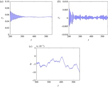
is a threshold value, beyond which VIVs are totally eliminated. A typical time history of the motions of the type A system with gap
 $G=0.5D$
is presented in figure 23. For time
 $t>300$
, the vibration in the streamwise direction approaches a stable value around
 $c_{x}=0.05$
, and the vibration in the cross-flow direction is in the range
 $-0.0015<c_{y}<0.0015$
. We also observe that the time trace of the fairing rotation takes negative values, suggesting a symmetry-breaking bifurcation for some cases.
Variation of the mean drag coefficient
 $C_{d}$
of the stationary configuration as a function of the Reynolds number, for three different systems: plain cylinder, homogeneous fairing and type A system.

Pressure coefficient contours at different spanwise and cross-flow planes for the type A system with gap
 $G=0.5D$
at different
 $\mathit{Re}$
: (a)
 $\mathit{Re}=100$
at
 $z=0.75$
, (b)
 $\mathit{Re}=100$
at
 $y=0$
, (c)
 $\mathit{Re}=500$
at
 $z=0.75$
, (d)
 $\mathit{Re}=500$
at
 $y=0$
, (e)
 $\mathit{Re}=1000$
at
 $z=0.75$
, and (f)
 $\mathit{Re}=1000$
at
 $y=0$
. The dashed line in the left plot denotes the planar cut presented in the plot on the right.

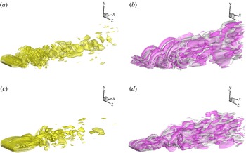
Figure 24 shows the flow structure in the wake by presenting isosurfaces of streamwise vorticity (
 ${\it\omega}_{x}=\pm 0.25$
) and spanwise vorticity (
 ${\it\omega}_{z}=\pm 0.55$
), and comparing them with the results of the homogeneous fairing system for the same conditions. For the homogeneous fairing, streamwise vorticity is very well organized and the flow patterns are very similar to those for flow past circular cylinders. For the type A system, the wake is widened in the gap region and the vortex street formation is delayed to a downstream position around
 $L=\text{3D}$
. Moreover, the vortex street is eliminated in the far wake, compared to the homogeneous fairing system.
Comparison of the
 $L_{2}$
norm of the motions of the structure and the related force coefficient for the homogeneous fairing system, and for the type A system with gap
 $G=0.5D$
at different
 $\mathit{Re}$
: (a) streamwise cylinder vibration, (b) cross-flow cylinder vibration, (c) rotation of fairing around the cylinder, (d) drag coefficient for the fairing part, (e) lift coefficient for the fairing, and (f) angular momentum of the fairing.

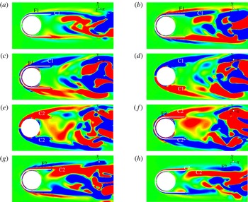
The streamwise vorticity contours at different
 $z$
slices for these two cases are shown in figures 25 and 26. We find that strong streamwise vorticity exists only between the parallel plates in the wake of the homogeneous fairing system. However, for a gap between fairings, vorticity is also generated at the front side of the fairing in the gap region, resulting in two antisymmetric vortex pairs, labelled C1 and C2 in figure 26. The strength of the C1 and C2 pair decreases, going from the gap centre towards the ends in the spanwise direction. We can see that there are two more vortex pairs, labelled F1 and F2, generated around the fairing, and their strongest part is at about
 $z=\pm 1.25$
. These vortex pairs interact with the vortex forming between the parallel plates in the wake, hence causing the previously coherent spanwise vorticity patterns, which feed and sustain the vortex street, to disorganize. This incoherent wake flow is the reason for the total elimination of the cylinder vibration and fairing rotation of the type A system.
Time history of the motions of the type A system with gap
 $G=0.5D$
at Reynolds number
 $\mathit{Re}=500$
: (a) streamwise displacement of the cylinder
 $c_{x}$
, (b) cross-flow displacement of the cylinder
 $c_{y}$
, and (c) rotational angle
 ${\it\theta}$
of the fairing.

Isosurfaces of spanwise vorticity
 ${\it\omega}_{z}=\pm 0.55$
(in yellow) and streamwise vorticity
 ${\it\omega}_{x}=\pm 0.25$
(in purple and grey) for (a,b) moving homogeneous fairing–cylinder system and (c,d) moving type A system with gap
 $G=0.5D$
, for friction coefficient
 $C_{f}=0.2$
and Reynolds number
 $\mathit{Re}=500$
.

Streamwise vorticity (
 $-0.25\leqslant {\it\omega}_{x}\leqslant 0.25$
) contours at different
 $z$
slices for a moving homogeneous fairing system at friction coefficient
 $C_{f}=0.2$
and Reynolds number
 $\mathit{Re}=500$
: (a)
 $z=-0.5$
, (b)
 $z=0$
and (c)
 $z=0.5$
.

Streamwise vorticity (
 $-0.25\leqslant {\it\omega}_{x}\leqslant 0.25$
) contours at different
 $z$
slices for a moving type A system with gap
 $G=0.5D$
at friction coefficient
 $C_{f}=0.2$
and Reynolds number
 $\mathit{Re}=500$
: (a)
 $z=-1.75$
, (b)
 $z=-1.25$
, (c)
 $z=-0.3$
, (d)
 $z=-0.25$
, (e)
 $z=0.25$
, (f)
 $z=0.3$
, (g)
 $z=1.25$
and (h)
 $z=-1.75$
.

Trajectories of motion for the fairing–cylinder system at
 $\mathit{Re}=500$
. The black line corresponds to a plain cylinder, the green line to a homogeneous fairing–cylinder system, and the red, blue and purple lines are for the fairing–cylinder system of type A with gap
 $G=0.5D$
at different values of the reduced velocity.

Next, we investigated the VIVs of the type A system for
 $\mathit{Re}=500$
at three different reduced velocity values,
 $U^{\ast }=3.5$
, 4.5 and 6, and compared the trajectory of motion with that of the plain cylinder and the homogeneous fairing system at the same
 $\mathit{Re}$
. From figure 27, we can see that the homogeneous fairing system can reduce the vibration in the cross-flow direction by 80 %, while the type A system with gap
 $G=0.5D$
essentially eliminates the vibrations, since the amplitude is smaller than 0.2 % of
 $D$
. At different reduced velocities, we find that the mean streamwise vibration amplitude is around
 $0.05D$
for
 $U^{\ast }=4.5$
and increases slightly with reduced velocity. In addition, for
 $U^{\ast }=3.5$
, 4.65 and 6, the oscillation frequencies for
 $c_{x}$
are 0.25, 0.2 and 0.167, respectively, while the oscillation frequencies for
 $c_{y}$
have the same value 0.2. Also, for all fairings with a gap, the mean rotation of the fairing around the cylinder is slightly negative, around 0.5°.
5.3. Fairing–cylinder system of type AB
In §§ 5.1 and 5.2, we investigated the simplified type A system. Typically, in industrial applications, several fairing segments of length 3–5 diameters are fitted on each riser section. We represent this herein with the simplified type AB fairing system with periodic boundary conditions at both ends, as shown in figure 2(c), to investigate the interaction of three adjacent fairings. Owing to the periodicity conditions, the two end fairings constitute effectively parts of the same fairing, while we introduce a second (middle) fairing;
 $C_{f}$
and
 $C_{g}$
will represent the friction coefficients for the two fairings, respectively. The equations of motion for the type AB system have been presented in § 3.2. In the following, we consider three cases with different
 $C_{f}$
and
 $C_{g}$
pairs: (a)
 $C_{f}=C_{g}=0.2$
, (b)
 $C_{f}=0.2$
,
 $C_{g}=0.25$
, and (c)
 $C_{f}=C_{g}=0.25$
. Additionally, we assume that the gap between fairings is
 $G=0.2D$
; two Reynolds numbers,
 $\mathit{Re}=100$
and 500, are considered.
To assess the effect of friction, we first obtain a converged flow for a moving type AB fairing using
 $C_{f}=C_{g}=0.2$
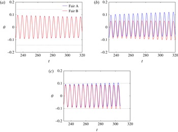
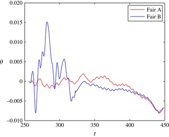
. Next, we change the friction coefficients to the values used in these three cases, and continue the simulations. Figure 28 presents time traces of the rotational angle of both fairings around the cylinder for the three different friction coefficient pairs. The red lines are for the first fairing (A), and the blue lines are for second fairing (B) in figure 2(c). The black dotted lines denote the rotational amplitude of a homogeneous geometry at the same Reynolds number,
 $\mathit{Re}=100$
, and friction coefficient,
 $C_{f}=0.2$
for the first case, and
 $C_{f}=0.25$
for the third case. For the same friction coefficients, the rotational response of a type AB fairing is very similar to type A, with the two fairings rotating at almost the same rate; see figure 28(a,c). However, for different friction coefficients,
 $C_{f}=0.2,C_{g}=0.25$
, the time traces of rotation for the two fairings, A and B, are totally different. The difference increases with time and the mean rotational angle deviates from the zero position, suggesting a symmetry-breaking bifurcation.
Time history of the rotation angles of the AB fairings (red lines, first fairing; blue lines, second fairing) at
 $\mathit{Re}=100$
: (a)
 $C_{f}=C_{g}=0.2$
; (b)
 $C_{f}=0.2$
,
 $C_{g}=0.25$
; and (c)
 $C_{f}=C_{g}=0.25$
. The dotted lines are for a homogeneous fairing–cylinder system for the same parameters.

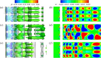
Flow structure for the type AB fairing at
 $\mathit{Re}=100$
in terms of: (a,c,e) isosurfaces of spanwise vorticity (
 ${\it\omega}_{z}=\pm 0.5$
) coloured in grey, and isosurfaces of streamwise vorticity (
 ${\it\omega}_{x}=\pm 0.3$
) coloured by pressure contour level; and (b,d,f) spanwise velocity shown at the centreline
 $y$
plane for type AB fairing at
 $\mathit{Re}=100$
with gap
 $G=0.2D$
; for (a,b)
 $C_{f}=C_{g}=0.2$
, (c,d)
 $C_{f}=0.2$
,
 $C_{g}=0.25$
, and (e,f)
 $C_{f}=C_{g}=0.25$
.

For AB fairings, streamwise vorticity contours (
 $-0.25\leqslant {\it\omega}_{x}\leqslant 0.25$
) at different
 $z$
slices at
 $z=-2.7,-2.2,-1.6,-1.0,-0.5$
(black horizontal lines in figure 29(a)), at
 $\mathit{Re}=100$
with gap
 $G=0.2D$
: (a)
 $C_{f}=C_{g}=0.2$
, (b)
 $C_{f}=0.2$
,
 $C_{g}=0.25$
, and (c)
 $C_{f}=C_{g}=0.25$
.

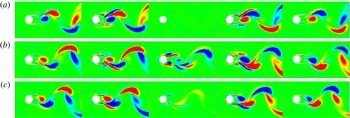
The difference in rotational response of the two fairings triggers different flow patterns behind each fairing of the type AB system. Figure 29 presents vorticity and velocity contours for three cases. The left column shows isosurfaces of spanwise vorticity (
 ${\it\omega}_{z}=\pm 0.5$
) in grey and isosurfaces of streamwise vorticity (
 ${\it\omega}_{z}=\pm 0.3$
) coloured by pressure contour level. The right column shows the spanwise velocity at the centreline in the
 $y$
plane, with the arrows denoting the spanwise flow direction. Moreover, figure 30 shows
 $z$
slices of streamwise vorticity at the positions
 $z=-2.7,-2.2,-1.6,-1.0,-0.5$
(black horizontal lines in figure 29
a). When the same friction coefficient is used for both fairings, the flow structure is similar for each fairing (see top and bottom rows of figure 29 and figure 30
a,c). The streamwise vorticity in the wake of fairing B (
 $z=-2.7,2.2$
) has the same pattern as the wake of fairing A (
 $z=-1.0,-0.5$
). In the gap region, there is either no or very small streamwise vorticity depending on the friction coefficient. However, when different friction coefficients are used,
 $C_{f}=0.2,C_{g}=0.25$
, the flow is changed, as shown in figures 29(c,d) and 30(b). Because of the larger rotational amplitude for fairing A, the streamwise vorticity in the wake of fairing A is much stronger than for fairing B. There is also significant streamwise vorticity in the gap region; see
 $z$
slice contour at
 $z=-1.6$
in the middle plot in figure 30(b). Unlike the flow for the type A fairing (figure 17), the flow separates in the gap region at the front (upstream) end of each fairing for the type AB system. Also the wake exhibits different patterns for the three cases, uniform versus A and AB. When the friction coefficient is the same across the span, i.e. for the first and third cases, the flow is converging in the gap region. With different friction coefficients,
 $C_{f}=0.2,C_{g}=0.25$
, the flow wake exhibits a high degree of interaction in the gap region, with the fluid gathering from fairing B to fairing A, or vice versa. The interaction is stronger in the wake around
 $L=\text{2D}$
(shown through a black circle).
Time history of the rotation angle in radians for each fairing of an AB system for different friction coefficients:
 $C_{f}=0.2$
,
 $C_{g}=0.25$
at
 $\mathit{Re}=500$
with gap
 $G=0.2D$
.

Next, we increase the Reynolds number to
 $\mathit{Re}=500$
for the type AB fairing and investigate the effect of the friction coefficients. Figure 31 shows the time history of the rotational angle for each fairing. There is significant difference in the response for time
 $t<300~\text{s}$
. Beyond this range, the two responses converge, approaching the same small negative value at around
 $t>375~\text{s}$
of about
 $-0.5^{\circ }$
. We can conclude that the effect of the friction coefficient of the fairings is negligible at higher Reynolds numbers. If we further investigate
 $z$
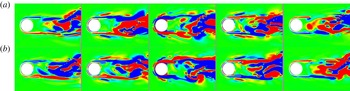
slices of streamwise vorticity at various positions along the span, as shown in figure 32, the flow is much different from that for the homogeneous fairing, as the development of organized spanwise vortices is significantly delayed, to about three of four diameters downstream. There are some similarities of the flow patterns with the type A system, but also major differences (see figure 25), as the wake is narrower and flow separation at the fairing is significantly reduced.
Streamwise vorticity contours (
 $-0.25\leqslant {\it\omega}_{x}\leqslant 0.25$
) at different
 $z$
slices of the type AB fairing system, at
 $z=-2.7,-2.2,-1.7,-1.0,-0.5$
in (a) and at
 $z=0.5,1.0,1.7,2.2,2.7$
in (b), at
 $\mathit{Re}=500$
for
 $C_{f}=0.2$
,
 $C_{g}=0.25$
and with gap
 $G=0.2D$
.

6. Conclusion
The principal result of the present study is that, for specific values of the gap between adjacent segments of U-shaped fairings attached on a cylinder in cross-flow, vortex-induced vibrations of the cylinder are suppressed, both in-line and cross-flow, and fairing rotations are also reduced to small values, resulting also in reduction of the drag coefficient by about 50 %. The effects of the gap increase with Reynolds number, by generating strong three-dimensionality in the flow, which disrupts the formation of coherent spanwise vortices until three of four diameters downstream in the wake.
We considered three different fairing geometries (figure 2): a homogeneous one, without a gap; a single gap with two adjacent fairings; and two gaps separating three adjacent fairings. Periodicity conditions are applied at the ends for all cases. The gap was changed from
 $0.2D$
up to
 $1.5D$
, and the Reynolds number from 100 to 10 000. We investigated the effect of the gap on the fluid forces and the translational and rotational motions of each system. While compared to a plain cylinder a homogeneous fairing system reduces drag by 15 %, a type A gap system can reduce the drag force coefficient by about 50 %. For a homogeneous fairing, the cross-flow amplitude is reduced by about 80 %, but for fairings with gaps longer than
 $0.5D$
, vibrations are almost completely eliminated.
As shown in figures 25, 26 and 32, while a uniform fairing delays the formation of spanwise vortical patterns by a length roughly equal to its streamwise length, a segmented fairing with gaps further delays coherent spanwise vortices by another two to four diameters, resulting in much smaller unsteady forces and hence negligible vibration.
The effect of friction in the fairing rotation was found in previous studies to be important, but we found a relatively small effect from friction, even when adjacent segments have different friction coefficients. In the latter case, however, symmetry may be broken, resulting in slightly rotated positions of adjacent fairings relative to each other, also affecting the flow symmetry.
Acknowledgements
The authors gratefully acknowledge the support by the Chevron–MIT University Partnership Program. F.F.X. also wishes to thank Drs X. Zheng and H. Babaee of the MIT Sea Grant Program for their thoughtful discussions of this paper.