



1. Introduction
Pervaporation is the process of drying of a liquid region by mass transport through a permeable medium. It occurs naturally in vascular plant leaves: water (or more precisely sap) is flowing in a network of veins, diffuses out of the veins through the leaf tissue and then evaporates at the surface of the leaf. This fascinating network of veins, called venation, can be very simple, with only one vein per leaf for Selaginella species, or can be very complex, with multiple connections between veins for flowering plants. A first aspect of this complexity is the hierarchy of vein sizes with main veins, secondary veins, tertiary veins and so forth. Another important aspect is the connectivity of the network, on which we focus here. When starting from the main vein where water is entering the leaf, veins can either: (i) split into several branches, (ii) reconnect, creating loops and a net-like reticulation of the network. In normal conditions water is flowing through the whole network. However, under severe drought, a cavitation bubble can appear and grow (Tyree & Sperry Reference Tyree and Sperry1989; Cochard Reference Cochard2006), the remaining water in the network then dries out, eventually disabling the leaf function. This mechanism may threaten a growing proportion of plants and trees in the context of global warming (Choat et al. Reference Choat, Brodribb, Brodersen, Duursma, López and Medlyn2018). In a different context, pervaporation through thin slabs of a water-permeable polymer, polydimethylsiloxane (PDMS) is used in so-called microevaporators in chemical engineering. It is useful because it ensures a homogeneous concentration of solutes or colloids and therefore a proper study of their phase diagrams (Walker & Beebe Reference Walker and Beebe2002; Eijkel, Bomer & van den Berg Reference Eijkel, Bomer and van den Berg2005; Leng et al. Reference Leng, Lonetti, Tabeling, Joanicot and Ajdari2006; Merlin, Salmon & Leng Reference Merlin, Salmon and Leng2012; Ziane et al. Reference Ziane, Guirardel, Leng and Salmon2015; Ziemecka, Haut & Scheid Reference Ziemecka, Haut and Scheid2015). However, despite the importance of these biological and chemical applications, pervaporation-induced flows in channel networks are little known, in contrast with the well-established field of pressure-driven flows in porous media.
To bridge this gap with a physical standpoint, our approach is to understand the drying using artificial channels in a permeable material, following the concept of biomimetic leaves incorporating a man-made microfluidic network in a porous material (Noblin et al. Reference Noblin, Mahadevan, Coomaraswamy, Weitz, Holbrook and Zwieniecki2008). Geometry and physical properties of the channels in the network are then well controlled. During drying, air invades the microfluidic network initially filled with water. The interfaces (menisci), separating air and remaining liquid, travel along all the branches of the network, and eventually either reach endpoints or merge with other ones.
The dynamics of moving menisci and expelled liquid has been observed in a two-dimensional (2-D) network of microchannels in the literature, but with different driving mechanisms: first, when a source of air pressure pushes liquid plugs out of a microfluidic network towards openings, for instance to study airway reopening in lungs (Song, Manneville & Baroud Reference Song, Manneville and Baroud2010; Song et al. Reference Song, Baudoin, Manneville and Baroud2011; Signe Mamba et al. Reference Signe Mamba, Magniez, Zoueshtiagh and Baudoin2018). Note the behaviour of these liquid plugs is similar to long droplets trapped in a network, causing them to potentially divide (Link et al. Reference Link, Anna, Weitz and Stone2004; Salkin et al. Reference Salkin, Schmit, Courbin and Panizza2013). There is also a similarity with the drainage of a large amount of liquid when pushed by another liquid (Armstrong & Berg Reference Armstrong and Berg2013). Second, the motion of menisci in networks has been studied when wetting drives the liquid, in the case of the spontaneous imbibition of a 2-D network by a wetting liquid (Sadjadi & Rieger Reference Sadjadi and Rieger2013). Here, the specificity of our study is that water constantly pervaporates all over the network, driving the flow.
The goal of this article is to provide a physical study on the dynamics of drying by pervaporation in channel networks. Such a dynamics has been previously studied and understood in single, straight channels (Noblin et al. Reference Noblin, Mahadevan, Coomaraswamy, Weitz, Holbrook and Zwieniecki2008; Ziane et al. Reference Ziane, Guirardel, Leng and Salmon2015; Dollet et al. Reference Dollet, Louf, Alonzo, Jensen and Marmottant2019). In this paper, we build up on this knowledge to study the most elementary network topologies: simple branches and loops; our aim is to provide a quantitative picture in these simple cases, which could be the ‘building block’ for more complex networks such as those encountered in natural leaves.
2. Materials and methods
2.1. Materials
In all our designs, there is a straight entrance channel into which drying starts. We added to all designs a circle of radius 1 mm at the root of the entrance channel. In plant leaves, embolism starts always in larger conduits (Brodribb, Bienaimé & Marmottant Reference Brodribb, Bienaimé and Marmottant2016a; Brodribb et al. Reference Brodribb, Skelton, McAdam, Bienaimé, Lucani and Marmottant2016b). The larger conduits are located on the larger veins, which occur at the base of the leaf in the petiole. Artificial embolism has therefore been proposed by injecting gas in the petiole of plant leaves (Hochberg et al. Reference Hochberg, Ponomarenko, Zhang, Rockwell and Holbrook2019), to mimic the development of embolism in natural conditions. In our set-up, the entrance channel thus mimics the main vein of leaves.
To study the effect of branching (without reconnections), we start with four designs with a single node where the entrance channel arrives and from where several straight branches, either two, three, four or five, emerge (figure 1). We shall henceforth call these designs single-node networks. All branches are of length  $L_b = 4.0\ \textrm {mm}$. For each single-node network, all channels (entrance channel and branches) have an equal angular distance from the node.
Snapshots of single-node networks, with  $(a)$ two,
 $(b)$ three,
 $(c)$ five and
 $(d)$ four branches.
 $(e)$ Transverse side view of the channels of width
 $w$ and height
 $h$ between a glass slide and a PDMS sheet of thickness
 $H$.
 $(\,f)$ Longitudinal side view of a branch. The meniscus, sketched as a vertical line inside the channel, separates a water-filled region on its right side and an air-filled region on its left side. The varying blue shade depicts the decreasing water vapour concentration
 $c_a$ in the air-filled region, also sketched by the red dashed curve which shows the decrease of
 $c_a$ over the characteristic length
 $L_g$. The green dashed arrows show the water flux leaving the channel by pervaporation through PDMS. The red dashed arrow shows the evaporation across the meniscus. The blue arrows inside the water-filled region represent the liquid flow induced by pervaporation.

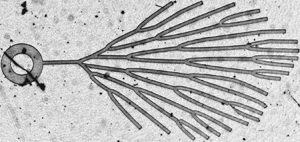
We then study branched networks with a larger number and a higher hierarchy of nodes, but at which each incoming branch subdivides in only two branches. First, we designed such a ‘tree’ with three levels of nodes (figure 2a). At each node, the two branches are separated by an angle of  $60^{\circ }$. Contrary to figure 1, not all the branches have the same length, to determine whether length variations have an effect on the drying kinetics. Finally, we study a natural vein network, namely the leaf of the fern Adiantum (Brodribb et al. Reference Brodribb, Bienaimé and Marmottant2016a). To do this, we adapted a mask drawn from the real leaf (Bienaimé Reference Bienaimé2016) and modified the channel widths such that they all have the same width
 $w = 100\ \mathrm {\mu }\textrm {m}$ (figure 2b), which is the common width of all the branched designs in the current study.
Snapshots of branched networks with more than one hierarchical level:  $(a)$ network with three hierarchical levels, and
 $(b)$ network from an Adiantum leaf (Brodribb et al. Reference Brodribb, Bienaimé and Marmottant2016a).

To study simple loops, we created four designs where the entrance channel splits at a first node, henceforth called the entrance node, into two channels making a circle of diameter  $2R_{\ell } = 4.3\ \textrm {mm}$, and reconnecting at a second node, henceforth called the exit node, from which a single straight terminal channel emerges. One of the loops is symmetric, i.e. the distance between both nodes is equal in the two channels connecting them (figure 3a), and the three others are asymmetric, with a shortest angular distance
 $\beta$ between the nodes, measured from the centre of the circle, equal to
 $120^{\circ }$ (figure 3b,d) or
 $60^{\circ }$ (figure 3c); this angle is obviously
 $180^{\circ }$ in figure 3(a). The terminal channel has a length
 $L_t = 3.0\ \textrm {mm}$ in figure 3(a–c), and 39 mm in figure 3(d), to determine whether
 $L_t$ has an effect on the drying dynamics.
Snapshots of the four designs with loops. In (a–c), the terminal channel is inside the circle merely to spare some space. (e) Sketch of the different elements of the loop.

We fabricated the channels based on all these designs as described in Dollet et al. (Reference Dollet, Louf, Alonzo, Jensen and Marmottant2019). We created masks from the designs using high-resolution printing. The channels were moulded in PDMS using standard soft lithography techniques. From the masks, we created a mould in a photoresistive material (SU8) on a silicon wafer. We mixed liquid PDMS (Sylgard 184, Dow Corning) with a curing agent in volumetric proportions  $9\,{:}\,1$. This mixture was degassed then spin coated on the mould at 300 revolutions per minute (r.p.m.) for 15 s then 900 r.p.m. for 40 s, to create an imprint of small thickness, and baked at
 $65\,^{\circ }\textrm {C}$ for one hour to reticulate the PDMS. This imprint was then bonded to a glass slide as follows. The bare glass slide was exposed for 30 s to a plasma, then the thin, flexible PDMS imprint was immediately deposited on top of the plasma-activated glass surface, carefully avoiding folding of the PDMS sheet. This simple procedure was sufficient to firmly bond PDMS and glass. We measured the channel thickness
 $h$ and the PDMS thickness
 $H$ using an interferometer. This is crucial because these thicknesses presented significant variations between different designs, despite the use of the same spin-coating parameters. The values of the thicknesses are tabulated in table 1. To speed up the measurements, we gathered the four single-node networks on one slide, the tree and Adiantum networks on a second one and all loops on a third one, at a distance large enough that diffusive interactions remain negligible. After figure 3 from Noblin et al. (Reference Noblin, Mahadevan, Coomaraswamy, Weitz, Holbrook and Zwieniecki2008), it is the case as soon as channels are separated by a distance of order
 $5\delta$, with
 $\delta = H - h$. In our case,
 $\delta \approx 60\ \mathrm {\mu }\textrm {m}$ (table 1), hence the distance between channels should be larger than 0.3 mm. In practice, the distance between different designs is larger than 1 mm.
Values of the channel thickness  $h$ and PDMS thickness
 $H$ measured for all the channels.

2.2. Methods
The experiments are performed as described in Dollet et al. (Reference Dollet, Louf, Alonzo, Jensen and Marmottant2019); we only repeat here the main steps. We opened the channels by manually cutting through the PDMS layer across the circle with a scalpel at the junction between the channels and the round part (these cuts are clearly visible in figures 1 and 2). Once the channels were water filled, we placed them under a dry atmosphere by imposing a constant dry air flux above the PDMS layer. Each channel progressively dried out, as menisci separating water from air advanced downstream through the channel from the roots to farther branches, until reaching the ends of the terminal branches. The motion of the menisci was imaged with a CCD camera.
To measure the location of the menisci as a function of time, we used the reslice operation of the freeware ImageJ and a home-made Matlab script. For each design, we draw a series of segmented lines following the middle of each channel, and we generate spatio-temporal diagrams along each line, for which we get the time evolution of the location of the menisci. Obtaining the velocity of the meniscus required us to take the discrete derivative of the length of the channel filled with water as a function of time. We chose to approximate the data for each meniscus, between its creation and annihilation (e.g. at a node), by a polynomial function of degree  $n\leq 9$. We chose the degree of the polynomial which gives the best coefficient of determination
 $R^{2}$ between the experimental data and the interpolating polynomial. We performed such an operation on each meniscus as long as it could be unambiguously defined between splitting or annihilation events (see next section).
3. Qualitative description of the experimental drying dynamics
3.1. Branched networks
In branched networks, the single meniscus in the entrance channel first moves until it splits at the entrance node, as shown in figure 4. In the single-node networks, each meniscus then moves until it annihilates against the terminal wall of each terminal branch. The dynamics in each branch has the same speed to within a few per cent (figure 4a). In the tree and Adiantum (figure 4b), there is a ‘cascade’ of consecutive splitting events as deeper nodes are reached by the different menisci, until the terminal branches are reached.
Snapshots of the progressive drying in (a) a single-node network with four branches, and (b) the Adiantum design. Darker areas in the networks represent dried parts of the channels, while lighter areas are still filled with water. Horizontal bars represent a length of 1 mm.

3.2. Loops
Drying in loops proceeds as follows. First, a single meniscus moves in the entrance channel until it splits in two menisci at the entrance node. Then we distinguish two cases. For the symmetric loop (figure 5a), the two menisci move almost symmetrically, until they merge at the exit node; the resulting meniscus in the terminal channel moves until it annihilates on the terminal wall of this channel, which ends the drying process. For the asymmetric loops (figure 5b), where the loop has a short and a long arm, the meniscus in the short arm reaches first the exit node, where it splits in two. We have then two disconnected water regions and three menisci: one water region is in the terminal channel, while the other, bounded by two menisci, is in the long arm, until both regions dry.
Snapshots of the progressive drying in (a) the symmetric loop, and (b) an asymmetric loop (the dynamics is qualitatively similar for the other asymmetric loops). Horizontal bars represent a length of 1 mm.

4. Theory
4.1. Drying dynamics for a single channel
In this section, we recall the main ingredients to model the drying dynamics by pervaporation in a single channel; see Dollet et al. (Reference Dollet, Louf, Alonzo, Jensen and Marmottant2019) for full details. This case is important because the drying models in networks, derived in §§ 4.2 and 4.3, elaborate on this simplest case, and also because it describes drying in each terminal branch of the various networks.
According to the experimental configurations, we consider a semi-infinite channel of width  $w$ and height
 $h$ between a glass slide and a PDMS layer of thickness
 $H$ (figure 1e), filled with water over a length
 $L$ between the channel extremity and an air/water meniscus. The outer air is at controlled relative humidity
 $RH = c_a^{{out}}/c_a^{{sat}}$ with
 $c_a^{{out}}$ the water vapour concentration in the outer air and
 $c_a^{{sat}}$ the water vapour concentration in saturated air; in our experiments,
 $RH = 0$. The channels dry because of water diffusion from the water-filled part of the channel to the outer air through the water-permeable PDMS. We showed in Dollet et al. (Reference Dollet, Louf, Alonzo, Jensen and Marmottant2019) that there are two contributions to the rate of decrease of the liquid volume: one by diffusion from the water–PDMS interface (
 $Q_{\ell }$), and one by evaporation from the meniscus (
 $Q_g$). Assuming that
 $L$ is much greater than
 $H$ and
 $w$, a condition generally met in practice because microfluidic channels are very slender, the water concentration profile in the PDMS between the water-filled part of the channel and the outer air is almost invariant along the channel length; hence,
 $Q_{\ell } = q_{\ell } L$ with
 $q_{\ell }$ the diffusive flux per unit length along the channel. We henceforth consider
 $Q_{\ell }$ and
 $Q_g$ as volumetric fluxes, and not molar fluxes as in Dollet et al. (Reference Dollet, Louf, Alonzo, Jensen and Marmottant2019), for simplicity; the main conclusions are unaffected by this choice. Equating the variation of volume of the water-filled part of the channel to the diffusive flux yields
 $hw\dot {L} = -q_{\ell } L + Q_g$, hence
 \begin{equation} \dot{L} + \frac{L + L_g}{\tau} = 0, \end{equation}
with
 \begin{equation} L_g = \frac{Q_g}{q_{\ell}} , \quad \tau = \frac{hw}{q_{\ell}} . \end{equation}
Equation (4.1) has the solution
 \begin{equation} L(t) = [L(t = 0) + L_g]\mathrm{e}^{-t/\tau} - L_g , \end{equation}
for  $t \leq \tau \ln [L(t = 0)/L_g]$, which is the time at which the channel fully dries. In Dollet et al. (Reference Dollet, Louf, Alonzo, Jensen and Marmottant2019), we derived analytical predictions for both
 $q_{\ell }$ and
 $Q_g$, hence, for
 $L_g$ and
 $\tau$, by solving first the two-dimensional diffusion problem in the cross-section of the water-filled part of the channel, then the three-dimensional diffusion problem in the PDMS and the air-filled part of the channel away from the meniscus. These calculations yield
 \begin{equation} L_g = \sqrt{\frac{\alpha D_a}{D_P}} \sqrt{\frac{hw}{\dfrac{w}{\delta} + \xi}} , \end{equation}
and
 \begin{equation} \tau = \frac{\rho}{D_P MC_P^{{sat}}(1 - RH)} \frac{hw}{\dfrac{w}{\delta} + \xi} , \end{equation}
with  $\alpha = 0.03$ the Henry constant quantifying the water affinity in PDMS (Harley, Glascoe & Maxwell Reference Harley, Glascoe and Maxwell2012),
 $D_a = 2\times 10^{-5}\ \textrm {m}^{2}\,\textrm {s}^{-1}$ the diffusivity of water vapour in air,
 $D_P = 10^{-9}\ \textrm {m}^{2}\,\textrm {s}^{-1}$ the diffusivity of water in PDMS (Watson & Baron Reference Watson and Baron1996),
 $\rho = 10^{3}\ \textrm {kg}\,\textrm {m}^{-3}$ the density of water,
 $M = 0.018\ \textrm {kg}\,\textrm {mol}^{-1}$ the molar mass of water,
 $C_P^{{sat}} = 40\ \textrm {mol}\,\textrm {m}^{-3}$ the saturation concentration of water in PDMS (Randall & Doyle Reference Randall and Doyle2005),
 $\delta = H - h$ the PDMS thickness between the channel top and the outer air and
 $\xi$ a dimensionless factor quantifying diffusion between the channel sidewalls and the outer air; under reasonable geometrical assumptions quantified in Dollet et al. (Reference Dollet, Louf, Alonzo, Jensen and Marmottant2019), it equals
 \begin{equation} \xi = \frac{2}{\rm \pi} \left[ \ln\frac{(H + \delta)h}{\delta^{2}} + \frac{H}{\delta} \ln\frac{H + \delta}{h} \right] . \end{equation}
In anticipation of what follows, it is worth reminding that the evaporative flux  $Q_g$ across the meniscus is related to water vapour in the air inside the channel: by Fick's law,
 $Q_g = -hwD_a \mathrm {d}c_a/\mathrm {d}x'|_{x' = 0}$, with
 $c_a$ the water vapour concentration field and
 $x'$ the distance from the meniscus. The spatial dependence
 $c_a(x')$ is itself related to the water transfer from the channel to the outer atmosphere through PDMS, hence it results from the coupled diffusion of water in air and in PDMS. In Dollet et al. (Reference Dollet, Louf, Alonzo, Jensen and Marmottant2019) we showed that
 $\mathrm {d}^{2} c_a/\mathrm {d}x'^{2} - c_a/L_g^{2} = 0$, with
 $L_g$ given by (4.4). Hence,
 $L_g$ can be interpreted as the typical distance over which air (and also PDMS) dries away from the meniscus (figure 1f). This distance is much larger than the typical cross-section dimensions: from (4.4),
 $L_g \approx M\sqrt {h\delta }$ with an amplification factor
 \begin{equation} M = \sqrt{\frac{\alpha D_a}{D_P}} , \end{equation}
which equals 30 with the aforementioned values for the different parameters. It is much larger than one, mostly because the diffusivity of water through PDMS is much less efficient than in air ( $D_P \ll D_a$), which ‘delays’ the drying of air inside the channel. This implies that the evaporation flux per unit area of the meniscus is much stronger (by a factor
 $M$) than the liquid pervaporation flux per unit area of the PDMS/channel interface. Yet, the contribution of liquid pervaporation to the total drying rate dominates if
 $Q_{\ell } > Q_g$ or if
 $L > L_g \approx M\sqrt {h\delta }$, which is the most common case in our experiments.
Increasing  $L_g$ implies weaker concentration gradients, which may at first sight lower
 $Q_g$ and contradict the very definition (4.2a,b) of
 $L_g$. This apparent contradiction is solved by the fact that increasing
 $L_g$ also implies increasing the prefactor relating
 $Q_g$ to the concentration gradient, relative to the prefactor relating
 $q_{\ell }$ to the concentration gradient.
The role of the evaporation through the meniscus into the air is somewhat reminiscent of the role of fins in heat transfer, which enhance the heat flux from a heated surface (Bejan Reference Bejan1993). In some sense, evaporation through the air channel acts as an extra effective ‘fin’ (in the sense of mass transfer, not of heat transfer) which adds up to the pervaporation flux from the PDMS/water interface.
4.2. Drying dynamics for branched channels
In branched channels, our experiments always begin with a single meniscus inside the entrance channel; as soon as the meniscus meets the first node of the network, it splits into two or more menisci, depending on the number of branches; and so forth for each of these menisci if they reach further nodes (figure 4).
We start our discussion with the single meniscus in the entrance channel at the beginning. Because the water-filled part spans multiple branches, the water concentration profile in the PDMS may differ from the single-channel case. More precisely, in the vicinity of a node, different branches are close enough to ‘compete’ for drying because they are coupled in the diffusion problem. However, as shown in Noblin et al. (Reference Noblin, Mahadevan, Coomaraswamy, Weitz, Holbrook and Zwieniecki2008), diffusive interactions between two neighbouring channels decay exponentially with  $H$ as the characteristic length scale. Hence, except if branches start from a node with a small separation angle, diffusive interactions thus fade away at a distance of order
 $H$ along each branch from a node. Therefore, provided the length of each branch between two consecutive nodes (or between a node and an extremity) is much larger than
 $H$, we can neglect the edge effect due to the nodes and extremities and consider, as in the case of a single channel, that the concentration profile between each water-filled branch and the outer air is invariant along the branch length, and similar to the single-channel case. In this case, the diffusive flux from the water–PDMS interface and the outer air still writes:
 $Q_{\ell } = q_{\ell } L$, with
 $L$ the total length of the water-filled branches ahead of the meniscus (figure 6a). Hence, the single meniscus in the entrance channel is predicted to obey (4.1) with solution (4.3).
In branched networks, (a) for a meniscus before a node,  $L$ is the total length of the water-filled branches ahead of the meniscus, here
 $L = L_0 + L_1 + L_2$. (b) Meniscus created after splitting in a node, having travelled a distance
 $\ell$ from the node where it has been created. (c) Sketch of the topology corresponding to the phase of the drying dynamics in loops shown in figure 5(a) (snapshots at
 $t = 15.6$ and 39 min) and figure 5(b) (snapshot at
 $t = 13.4\ \textrm {min}$).

Let us now consider one meniscus inside one of the branches, obtained after a splitting event. From the previous discussion, we still have  $Q_{\ell } = q_{\ell } L$, with
 $L$ the total length of the water-filled branches ahead of the meniscus. For simplicity, we shall henceforth call this quantity
 $L$ the ‘water length’. However, if the distance
 $\ell$ travelled by the meniscus from the node where it has been created (figure 6b) is smaller than, or of the order of magnitude of
 $L_g$, the water concentration profile behind the meniscus, responsible for the contribution
 $Q_g$ (see § 4.1), is affected by the presence of the node. In other words, menisci issued from a given splitting event interact over a range of order
 $L_g$, which is much larger than
 $H$ or
 $w$ (see § 4.1). Hence, in the case
 $\ell \lesssim L_g$, we cannot use the single-channel prediction for
 $Q_g$.
In appendix A, we derive a prediction for the diffusive flux from the meniscus accounting for this interaction. We show in § 5.1.1 that the discrepancy between this prediction and the single-channel prediction remains small in the parameter range of our experiments. Hence, to simplify the forthcoming discussion of our experiments, we shall simply use (4.1) as a prediction with  $L$ the total length of the water-filled branches ahead of the meniscus under consideration, unless explicitly stated.
4.3. Drying dynamics for loops
The key difference between branched channels without loops, on the one hand, and loops on the other hand, is the following. In branched channels, each connected water region is bounded by one meniscus. On the contrary, once the meniscus has split at the entrance node of the designs with loops, there is a connected water region bounded by two menisci (snapshots at  $t = 15.6$ and 39 min in figure 5(a), and at
 $t = 13.4\ \textrm {min}$ in figure 5b). However, the model developed in § 4.2 predicts the rate of drying of a given connected water region, but not how such a rate determines the individual velocity of two (or more generally multiple) menisci bounding that region.
To go one step further, we must delve into the details of the hydrodynamics driven by pervaporation. We start with the simplest case, namely the single channel with a water region of length  $L$ bounded by one meniscus and one terminal wall, a case for which pervaporation-induced flow is well documented (Verneuil, Buguin & Silberzan Reference Verneuil, Buguin and Silberzan2004; Randall & Doyle Reference Randall and Doyle2005; Leng et al. Reference Leng, Lonetti, Tabeling, Joanicot and Ajdari2006). We denote by
 $x$ the streamwise axis, with
 $x = 0$ at the wall and
 $x = L$ at the meniscus and
 $u(x,t)$ the velocity, averaged over the cross-section. Since
 $q_{\ell }$ is the flux of water leaving the channel per unit length, water conservation inside the channel (assuming incompressible flow) implies that
 $\partial u/\partial x = -q_{\ell }/hw$. To integrate this equation, we use the classical impermeability condition at the terminal wall
 \begin{equation} u(0,t) = 0 , \end{equation}
to get
 \begin{equation} u = -\frac{q_{\ell}}{hw} x . \end{equation}
It is worth noting that  $u(L,t)\neq \dot {L}(t)$, because of the evaporation flux
 $Q_g$ leaving the meniscus; this is an illustration of Stefan flows. The correct relationship is
 \begin{equation} u(L,t) = \dot{L} + \frac{Q_g}{hw} . \end{equation}
Moreover, the impermeability assumption (4.8) is, strictly speaking, wrong because of the ‘leakiness’ of the PDMS walls. However, because of the large value of the amplification factor (4.7), the water velocity across the terminal wall remains small in comparison to  $Q_g/hw$, which justifies using (4.8) as a first approximation. This also enables us to neglect the velocity across the walls everywhere, hence we can use a no-slip boundary condition there, and we can also neglect the transverse pressure gradients compared to the longitudinal pressure gradient. Therefore, we can use the Poiseuille law relating the average velocity to the pressure gradient for a laminar flow in a rectangular channel
 \begin{equation} u = -\frac{\mathcal{S}}{\eta} \frac{\partial p}{\partial x} , \end{equation}
with the section  $\mathcal {S}$ equal to (see e.g. Bruus Reference Bruus2007)
 \begin{equation} \mathcal{S} = \frac{1}{12} h^{2} - \frac{16}{{\rm \pi}^{5}} \frac{h^{3}}{w} \sum_{n = 0}^{\infty} \frac{1}{(2n+1)^{5}} \tanh \frac{(2n+1){\rm \pi} w}{2h} . \end{equation}
The boundary condition for the pressure field comes from the Laplace pressure jump across the meniscus
 \begin{equation} p_a - p(L,t) = \gamma\kappa , \end{equation}
with  $p_a$ the atmospheric pressure,
 $\gamma$ the surface tension and
 $\kappa$ the curvature, counted positive if the centre of curvature is on the air side. The curvature depends on the width and height of the channel, and on the contact angles of water on both glass and PDMS; it is positive with our convention because both contact angles are smaller than
 $90^{\circ }$, as can be seen from the meniscus curvature in the snapshots. From (4.9) and (4.11), we thus get the pressure field in a single channel
 \begin{equation} p(x,t) = p_a - \gamma\kappa - \frac{\eta q_{\ell}}{2hw\mathcal{S}} (L^{2} - x^{2}) . \end{equation}
We now consider a connected water region with two menisci. If it spans a single channel, in particular the long arm of a loop as in figure 5(b) (see the snapshot at  $t = 47.5\ \textrm {min}$), its drying dynamics is very similar to the single-channel case discussed in § 4.1, except that the water flux
 $Q_g$ across a given meniscus must be counted twice. Hence instead of (4.1), we have
 \begin{equation} \dot{L} + \frac{L + 2L_g}{\tau} = 0 , \end{equation}
provided that the distance travelled by each meniscus from the node where it has been created is smaller than, or of the order of magnitude of  $L_g$ (see the discussion of § 4.2). Under this assumption, the dynamics of each of the two menisci must be similar and they must move at the same velocity.
If a connected water region with two menisci spans three ‘branches’ connecting at a node, as in figure 5(b) (see the snapshot at  $t = 13.4\ \textrm {min}$), we must consider each branch. For the terminal channel of length
 $L_0$, we simply adapt (4.8) and (4.9):
 $u_0(L_0,t) = 0$ and
 $\partial u_0/\partial x_0 = -q_{\ell }/hw$ (see figure 6c for the orientation of the axis); in particular, we get
 $U_0 \equiv u_0(0,t) = q_{\ell } L_0/hw$. For each of the two parts between the node and one meniscus,
 $\partial u_i/\partial x_i = -q_{\ell }/hw$ (for
 $i = 1, 2$), hence
 \begin{equation} u_i(x_i,t) = U_i - \frac{q_{\ell}}{hw} x_i , \end{equation}
where  $U_i$ is the velocity in channel
 $i$ at the node. One relation between the two unknowns
 $U_1$ and
 $U_2$ comes from the flux conservation at the node
 \begin{equation} U_0 + U_1 + U_2 = 0 . \end{equation}
To get a second relation, we compute the pressure difference between the node and each of the two menisci
 \begin{equation} \int_0^{L_i} \frac{\partial p_i}{\partial x_i} \, \mathrm{d} x_i = p_a - \gamma\kappa - p_0 , \end{equation}
for  $i = 1, 2$, after (4.13), and denoting
 $p_0$ the pressure at the node. We also have
 \begin{equation} \int_0^{L_i} \frac{\partial p_i}{\partial x_i} \, \mathrm{d} x_i = -\frac{\eta}{\mathcal{S}} \int_0^{L_i} u_i \, \mathrm{d} x_i = -\frac{\eta}{\mathcal{S}} \left( -\frac{q_{\ell}}{2hw} L_i^{2} + U_i L_i \right) , \end{equation}
from (4.11) and the expression (4.16) of the velocity, whence the second relation between  $U_1$ and
 $U_2$
 \begin{equation} -\frac{q_{\ell}}{2hw} L_1^{2} + U_1 L_1 = -\frac{q_{\ell}}{2hw} L_2^{2} + U_2 L_2 . \end{equation}
Solving the system (4.17) and (4.20), we get
 \begin{align} U_1 = \frac{q_{\ell}}{hw} \left[ \frac{1}{2} (L_1 - L_2) - \frac{L_2}{L_1 + L_2} L_0 \right] , \quad U_2 = -\frac{q_{\ell}}{hw} \left[ \frac{1}{2} (L_1 - L_2) + \frac{L_1}{L_1 + L_2} L_0 \right] . \end{align}
We can finally predict the velocity of the menisci. Inserting  $U_1$ and
 $U_2$ in (4.16), taking into account that
 $\dot {L}_i = u_i(L_i,t) - {Q_g}/{hw}$ from (4.10) and using (4.2a,b), we get
 \begin{equation} \left. \begin{gathered} \dot{L}_1 = -\frac{1}{\tau} \left[ \frac{1}{2} (L_1 + L_2) + \frac{L_2}{L_1 + L_2} L_0 + L_g \right] ,\\ \dot{L}_2 = -\frac{1}{\tau} \left[ \frac{1}{2} (L_1 + L_2) + \frac{L_1}{L_1 + L_2} L_0 + L_g \right]. \end{gathered} \right\} \end{equation}
These predictions deserve some comments. First,  $\dot {L}_i < 0$, which is of course consistent with the loss of liquid water upon drying. Second, the largest velocity
 $|\dot {L}_i|$ is predicted to occur in the shortest arm. This is also expected, because the same pressure drop drives the liquid between the node and each meniscus. Third, when
 $L_0 = 0$, the equations are compatible with (4.15) when setting
 $L = L_1 + L_2$. Fourth, the dynamics becomes nonlinear, contrary to (4.1) and (4.15).
We now solve (4.22). As expected, the sum of the lengths obeys a simple equation
 \begin{equation} \dot{L}_1 + \dot{L}_2 = -\frac{L_1 + L_2 + L_0 + 2L_g}{\tau} , \end{equation}
with solution  $L_1 + L_2 = (L_{10} + L_{20} + L_0 + 2L_g)\mathrm {e}^{-t/\tau } - (L_0 + 2L_g)$, denoting the initial conditions:
 $L_i(t = 0) = L_{i0}$ for
 $i = 1, 2$. Inserting this solution in (4.22), we find that the difference of the lengths obeys a linear equation, albeit with a time-dependent coefficient
 \begin{equation} \dot{L}_1 - \dot{L}_2 = \frac{L_0}{\tau} \frac{L_1 - L_2}{(L_{10} + L_{20} + L_0 + 2L_g)\mathrm{e}^{-t/\tau} - (L_0 + 2L_g)} . \end{equation}
This is a separable equation which is easy to solve, and which yields
 \begin{align} L_1 - L_2 &= (L_{10} - L_{20}) \left[ \frac{(L_{10} + L_{20} + L_0 + 2L_g)\mathrm{e}^{-t/\tau} - (L_0 + 2L_g)}{L_{10} + L_{20}} \right]^{L_0/(L_0 + 2L_g)}\nonumber\\ &\qquad \times \exp \left( -\frac{L_0}{L_0 + 2L_g} \frac{t}{\tau} \right). \end{align}
Of course, this solution holds only as long as both lengths remain positive, which ceases when the length in the shortest arm decreases to zero. This occurs at a critical time which must be solved numerically using the expressions of  $L_1$ and
 $L_2$.
5. Experiments
Having derived all theoretical tools to predict the dynamics in our elementary networks, we now proceed to a quantitative description of the experiments, and compare them to our predictions.
5.1. Branched networks
5.1.1. Single-node networks
We begin by measuring the drying dynamics in single-node networks (figure 1). The distance travelled by the menisci is plotted as a function of time in figure 7; the time origin here is somewhat arbitrary, corresponding to the beginning of the camera recording. The distance increases with time, as drying proceeds. For a given number of branches, all branches show a similar dynamics, with a drying velocity decreasing with increasing distance. The striking feature of the drying dynamics is a velocity jump: the meniscus velocity is larger in the main channel than in the branches, the jump being larger at increasing number of branches (figure 7).
Drying dynamics in branched networks. Displacement of the meniscus from the origin as a function of time for networks with  $(a)$ two,
 $(b)$ three,
 $(c)$ four and
 $(d)$ five branches. Symbols correspond to different branches as sketched on each panel: round symbols correspond to the main channel, other symbols correspond to branches. The origin is marked with a filled black circle.

The origin of the jump can be qualitatively explained from the discussion in § 4.2, illustrated in figure 6(a,b). The water length from the meniscus coming from the entrance channel, as it arrives at the node, equals  $NL_b$ with
 $L_b$ the length of each branch. As it splits into
 $N$ menisci, each of these has its own water length equal to the branch length
 $L_b$. More quantitatively, the dynamics of all menisci should obey (4.1). To test this idea, we plot the meniscus velocity as a function of the water length for all menisci in figure 8(a). This shows indeed that all data follow a common trend, which is well fitted by a straight line. The entrance channels show small deviations from this trend. We have no clear explanation for these deviations, but they may be due to the somewhat uncontrolled opening of the channels by scalpel cutting (see § 2.2). However, they remain within 10 % from the straight line, suggesting that the simple model (4.1) already captures the dynamics of drying in branched channels with good accuracy. The value of the fitting parameters will be discussed in § 6.1 for all experiments.
 $(a)$ Velocity of the meniscus as a function of the water length, in the main channel of the network of two (
 $\circ$), three (
 $*$), four (
 $+$) and five (
 $\times$) branches, and in the branches (triangles). The line is a linear fit of all data, with best fitting parameters in (4.1):
 $\tau = 1.8 \times 10^{3}\ \textrm {s}$ and
 $L_g = 1.1\ \textrm {mm}$.
 $(b)$ Velocity of the meniscus as a function of the water length, in branches of the network of two (
 $\triangle$), three (
 $\triangledown$), four (
 $\triangleright$) and five (
 $\triangleleft$) branches. The curves are fits of the data for two (plain curve), three (dashed curve), four (dotted curve) and five (dash-dotted curve) branches by (5.1) and (5.2), with best fitting parameters:
 $\tau = 1.7 \times 10^{3}\ \textrm {s}$ and
 $L_g = 1.1\ \textrm {mm}$. The straight line corresponds to (4.1) using the latter two parameters.

As discussed at the end of § 4.2, we should in principle not use the single-channel version of the flux  $Q_g$ from the meniscus for the dynamics inside the branches, but rather the expression (A 8) derived in appendix A, which accounts for the coupled evaporation from different menisci issued from the same node. Hence, (4.1) should be replaced by
 \begin{equation} \dot{L} + \frac{L + fL_g}{\tau} = 0 , \end{equation}
with a factor  $f$ given by, after (A 8) and since
 $L_b = \ell + L$ (figure 6b)
 \begin{equation} f = \frac{\cosh[(L_b - L)/L_g] + N\sinh[(L_b - L)/L_g]}{\sinh[(L_b - L)/L_g] + N\cosh[(L_b - L)/L_g]} . \end{equation}
To quantify the magnitude of this correction, we focus on the data for the branches, and we fit them by (5.1) and (5.2), using  $\tau$ and
 $L_g$ as free fitting parameters. The results are shown in figure 8(b). They show indeed a small deviation from a linear relationship between the meniscus velocity and the water length as the latter tends towards the branch length, i.e. as the meniscus is close to the node. This is in qualitative agreement with our model of evaporation coupling of the menisci, even though the agreement is not fully quantitative, perhaps because the hypotheses underlying the model (notably that
 $w$ and
 $H$ are much lower than other lengths under consideration) become questionable in the range of lengths where evaporation coupling is significant. However, the main result from this analysis is that evaporation coupling has only a small effect on the velocity of the menisci inside the branches, because the difference of velocity is only 10 % lower with coupling than without (compare the straight lines and the curves in figure 8b). Hence, to simplify the forthcoming discussion of our experiments, we shall simply use (4.1) as a prediction with
 $L$ the total length of the water-filled branches ahead of the meniscus under consideration.
5.1.2. Multinode networks
Overall, the results on single-node networks suggest a strong correlation between the meniscus velocity and the water length. We further test this idea by studying more complex branched channels. We consider first the ‘tree’ network of figure 2(a). We first plot the distance travelled by the menisci as a function of time in figure 9(a). This graph shows that at each node, there is a jump of velocity, consistent with the previous observations of single-node networks. Moreover, there is a signature of the asymmetry of the eight terminal branches: the drying occurs in a shorter time, but with a lower velocity, in the two short branches (inset of figure 9a). According to the previous discussion, we measure the meniscus velocity and water length in the main channel and in each branch, and we plot the dependency between these two quantities in figure 9(b). This shows that the data are gathered in four subgroups, depending on the level of the branch considered inside the tree; as in the previous case, the gaps between each subgroup are associated with a velocity jump as a meniscus splits in two at each node. Moreover, the data collapse very well onto a straight line, which confirms that the simple model (4.1) describes well the drying dynamics even in cases with multiple nodes.
Drying dynamics in the network of figure 2(a).  $(a)$ Displacement of the meniscus from the origin as a function of time (inset: zoom on the terminal branches).
 $(b)$ Velocity of the meniscus as a function of the water length, and sketch of all branches with their symbols used in this figure. The line is a linear fit of all data, with best fitting parameters giving in (4.1):
 $\tau = 2.9 \times 10^{3}\ \textrm {s}$ and
 $L_g = 0.8\ \textrm {mm}$.

We finally consider the Adiantum design (figure 2b). Since there are many edges (45 in total), we measure only the average velocity in each edge, and we retain the standard deviation of velocity as an error bar. We plot the meniscus velocity as a function of the water length in figure 10. All data collapse again very well on a single straight line, with only one significant outlier. This collapse is all the more remarkable that the Adiantum design does not really obey the model approximations; because it comprises many veins, which are not all slender, and they are close enough that diffusive interactions may become significant.
Velocity of the meniscus as a function of the water length in the different edges of the Adiantum network. The line is a linear fit of all data, with best fitting parameters giving in (4.1):  $\tau = 3.0 \times 10^{3}\ \textrm {s}$ and
 $L_g = -0.4\ \textrm {mm}$.

5.2. Loops
5.2.1. Meniscus position and water length
In the branched networks without reconnections, we have quantified the position of the menisci by the distance travelled from the origin, which was unambiguous. Conversely, in loops, there are several possible choices to quantify the position  $x$ of a meniscus. We proceed as follows, and as illustrated in figure 11(a); in each case, we also relate
 $x$ to the water length
 $L$ or to the quantities
 $L_1$ and
 $L_2$ previously introduced.
(a) Snapshots of the different menisci in a loop, superimposed with the symbols used to plot their positions in panels (b,c). (i) Meniscus coming from the entrance channel, and splitting at the entrance node into (ii) two menisci in each branch of the loop. Then the meniscus in the short arm splits at the exit node and (iii) the remaining water splits in two disconnected regions, one in the terminal channel and the other, bounded by two menisci, in the long arm. (b,c) Dynamics of individual menisci in two asymmetric loops: time evolution of the different menisci (b) in the loop of figure 3(b,c) in the loop of figure 3(c); the menisci are distinguished by different symbols and colours as shown by in panel (a). The lines are the predictions of the dynamics of each meniscus by the model of § 4.3, with best fitting parameters: (b)  $\tau = 2.6 \times 10^{3}\ \textrm {s}$ and
 $L_g = 1.7\ \textrm {mm}$ and (c)
 $\tau = 2.5 \times 10^{3}\ \textrm {s}$ and
 $L_g = 1.7\ \textrm {mm}$.

For the meniscus in the terminal channel, we use the distance  $s$ from the end of the channel (figure 11a,iii). In this case, we thus have simply:
 $x = s$ and
 $L = s$.
When there is one meniscus per arm, for the meniscus in the short arm, we set  $x = L_t + R_{\ell } \theta$, where we recall that
 $L_t$ the length of the terminal channel,
 $R_{\ell }$ the radius of the loop and where
 $0 \leq \theta \leq \beta$ is the angular distance between the meniscus and the exit node (figure 11a,ii), and
 $\beta$ the small angle between both nodes. For the menisci in the long arm, we set
 $x = L_t + R_{\ell } \theta '$ with
 $0 \leq \theta ' \leq 2{\rm \pi} - \beta$ the angular distance between the meniscus and the exit node (figure 11a,ii). We thus have:
 $L = L_t + R_{\ell } (\theta + \theta ')$. For these menisci, the lengths
 $L_1$ and
 $L_2$ introduced in § 4.3 are proportional to the angular distances:
 $L_1 = R_{\ell } \theta '$ and
 $L_2 = R_{\ell } \theta$. When there are two menisci in the long arm (figure 11a,iii), we define their position
 $x_{\pm } = L_t = R_{\ell } \theta _{\pm }$ (with
 $\theta _- \leq \theta _+$), and the water length of the region between them is
 $L = R_{\ell } (\theta _+ - \theta _-)$.
For the meniscus in the entrance channel, we set  $x = L_t + R_{\ell } \beta + s$, and we have:
 $L = L_t + 2{\rm \pi} R_{\ell } + s$ (figure 11a,i).
5.2.2. Symmetric loop
In the symmetric loop, the position of each meniscus is plotted as a function of time in figure 12(a). The dynamics of the meniscus in the entrance channel and that in the terminal channel is smooth, and as before, the velocity of each meniscus decreases in time. The two menisci in the arms of the loop do not behave perfectly symmetrically, and their displacement curves show some irregular inflections, but the difference remains small and they reach the exit node simultaneously. As for the single-node branched networks, there is a velocity jump as the meniscus splits in two at the entrance node, the velocity of each of the two new menisci being smaller. Interestingly, the opposite velocity jump is observed at the exit node: the velocity of the meniscus in the terminal channel is greater than that of the two menisci merging at the exit node.
Drying dynamics in the symmetric loop: (a) time evolution of the position of the menisci, in the entrance channel ( $\circ$), in both arms (
 $\square$ and
 $\triangleright$) and in the terminal channel (
 $\lozenge$). The curves are fits by (4.3) and (4.22), with best fitting parameters:
 $\tau = 2.6 \times 10^{3}\ \textrm {s}$ and
 $L_g = 2.1\ \textrm {mm}$. (b) Drying velocity
 $|\dot {L}|$ as a function of the water length in the different phases of drying in the symmetric loop. The new symbol (
 $*$) as compared to panel (a) corresponds to the water length of the region bounded by two menisci, one in each arm. The lines are fits by (4.1) and (4.23).

We now compare this experimental dynamics with our model. The dynamics of the entrance and the terminal meniscus is simple, since each is the only meniscus present in the network during their period of existence; they should obey (4.3), provided the water length is defined as before. When there are two menisci in the symmetric loop, the model of § 4.3 show that they should have the same velocity; it is a special case of the coupled equations (4.22). The fitting parameters  $\tau$ and
 $L_g$ are taken once and for all the data (and not separately for each curve). Figure 12(a) shows a good agreement between the experiments and the predictions, except for the aforementioned small difference between the two menisci in the two arms. Furthermore, the sum of their velocity, which is the drying velocity
 $|\dot {L}|$, is predicted to follow (4.23), which is similar to (4.1) except for the prefactor of
 $L_g$, which counts the number of menisci bounding the drying water region. Therefore, we plot the drying velocity
 $|\dot {L}|$ as a function of the water length in figure 12(b). Indeed, the data gather into three subgroups, with the same slope as expected from (4.1) and (4.23), but with an offset when there are two menisci. More precisely, the data are very well fitted by (4.1) and (4.23).
5.2.3. Asymmetric loops
For the asymmetric loops, the three cases described for the symmetric loop, namely (i) the meniscus in the entrance channel, (ii) one meniscus in each arm of the loop and (iii) the meniscus in the terminal channel, are supplemented with a fourth case: the existence of a water region bounded by two menisci in the long arm. For all these cases, we plot the experimental dynamics of each single meniscus in figure 11(b,c) for two of the asymmetric loops, and we compare it to the predictions of § 4.3. As discussed in that section, the dynamics of the menisci in the entrance and terminal channel is predicted to obey (4.1). When there is one meniscus in the short arm and another in the long arm, their dynamics is predicted to obey the coupled equations (4.22), until the meniscus in the short arm reaches the exit node. Finally, when there is a water region in the long arm bounded by two menisci, its dynamics is predicted to follow (4.15) where each meniscus contributes to half of the velocity. Figure 11(b,c) shows that, while the agreement between experiments and theory is good for the meniscus in the entrance and terminal channels, and still rather good for the two menisci bounding a water region in the long arm, there is a significant discrepancy in the phase of drying where there is one meniscus per arm. While our model predicts that the meniscus in the short arm should have the largest velocity, the contrary occurs in figure 11(c). In figure 11(b), even if the meniscus in the short arm is faster, the difference of velocities between the two menisci is much larger than the prediction. A likely origin of this discrepancy is discussed in § 6.2.
To go further, we plot the water length of the different water regions as a function of time in figure 13(a,c,e), and the drying velocity  $|\dot {L}|$ as a function of the water length in figure 13(b,d,f). This shows that, in the spite of the discrepancy for individual menisci, the drying velocity of the water region bounded by a meniscus in the short arm and another in the long arm is well captured by the model. Another striking feature is the significantly larger drying velocity, for a given water length, of the water region in the long arm compared to the water region in the terminal channel. This is perhaps the best illustration of the influence of the contribution of the menisci to the drying of a given water region. For instance, in the asymmetric loop of figure 3(b), even though it is initially twice shorter, the water region in the terminal channel takes almost the same time to dry as the water region in the long arm. Comparing figures 12(a) and 13(a,c) also shows that, for the same total channel length, the total drying time is shorter in asymmetric loops compared to the symmetric one. To compare these data with the model, we proceed as for the symmetric loop, with as new feature the water region in the long arm. Since it is bounded by two menisci, its dynamics should obey (4.15). Hence, as previously, we plot the velocity of the meniscus, or the sum of the velocity of the menisci if there are two, as a function of the water length, in figure 13(b,d,f). Here again, the data gather in four subgroups, with the same slope but with an offset correlated to the number of menisci. The data are well fitted by (4.1), (4.15) and (4.23) with
 $\tau$ and
 $L_g$ as fitting parameters taken once and for all the data; the agreement is slightly less good than for the symmetric loop, but the deviations remain relatively small.
Drying dynamics in the asymmetric loops of figure 3(b) (a,b), 3(c) (c,d) and 3(d) (e,f). (a,c,e) Time evolution of the water length, for the meniscus in the entrance channel ( $\circ$), for two menisci with one in each arm of the loop (
 $*$), for the meniscus in the terminal channel (
 $\square$) and for the water region in the long arm (
 $\triangle$). (b,d,f) Drying velocity
 $|\dot {L}|$ as a function of the water length in the different phases of drying. The lines are fits by (4.1), (4.15) and (4.23), with best fitting parameters: (b)
 $\tau = 2.6 \times 10^{3}\ \textrm {s}$ and
 $L_g = 1.7\ \textrm {mm}$, (d)
 $\tau = 2.5 \times 10^{3}\ \textrm {s}$ and
 $L_g = 1.7\ \textrm {mm}$ and (f)
 $\tau = 2.6 \times 10^{3}\ \textrm {s}$ and
 $L_g = 2.7\ \textrm {mm}$.

We notice finally that there are no qualitative differences between the three asymmetric loops. In the most asymmetric loop (figure 3c), the duration of the phase of coexistence of two menisci in the two arms decreases, while the water region created in the long arm after meniscus splitting at the exit node is initially longer and takes a longer time to dry, as expected. For a longer terminal channel, the durations of the phase of coexistence and of the water region in the long arm are both reduced.
6. Discussion
In this section, we focus on two further aspects of our study. First, we must now discuss the values of the fitting parameters  $\tau$ and
 $L_g$, especially the first one, which gives the typical drying time. Second, we shall discuss the discrepancy observed between the experiments and the model in the specific case of individual menisci in the loops.
6.1. Values of the fitting parameters
The fits of all our data are related to the two same parameters: the typical drying time  $\tau$, and a length
 $L_g$ related to the contribution of the meniscus to drying. We summarise the values of these parameters in table 2, together with their theoretical predictions using (4.4) and (4.5).
Values of the fitting parameters  $\tau$ and
 $L_g$ for all the channels, and their theoretical predictions.

The value of the typical time  $\tau$ shows some dispersion: it is lowest for the single-node networks, highest for the tree and Adiantum and intermediate for the loops; the values for the tree and Adiantum on the one hand, and for the various loops on the other hand, are very similar. This apparent dispersion is actually well correlated with the difference in thickness for the different designs (table 1). Indeed, our model predicts the following dependence of
 $\tau$ on the geometrical parameters, see (4.5):
 $\tau \propto hw/(\xi + w/\delta )$. Therefore, we plot
 $\tau$ as a function of
 $hw/(\xi + w/\delta )$ in figure 14. The data then align correctly on an affine trend, although the data for the single-node networks lie slightly below the line. Moreover, the slope of the affine fit, equal to
 $1.9\ \textrm {s}\,\mathrm{\mu}\textrm {m}^{-2}$, compares favourably with the prediction, from (4.5):
 $\rho /D_P MC_P^{{sat}} = 1.4\ \textrm {s}\,\mathrm {\mu }\textrm {m}^{-2}$, although it is somewhat higher (likewise, fitted values of
 $\tau$ are larger than theoretical estimates). However, the values of
 $C_P^{{sat}}$ and
 $D_P$ taken from the literature are known only with poor precision. Hence, to get a better check, we have repeated experiments on single channels, on two different chips, performed with the same protocol as for the various networks. Fits of the resulting curves
 $L(t)$ (not shown) by (4.3) yield fitting values for
 $\tau$ which are added on figure 14 as cross symbols. These single-channel data follow the same trend as the data for the networks to within a few per cent. This constitutes a further validation of our models, and of their extension from single channels to networks.
Value of the fitting parameter  $\tau$ (see table 2) as a function of the geometrical parameter
 $hw/(\xi + w/\delta )$. The line is an affine fit of the data for networks (round symbols), with a value of the slope
 $1.9\ \textrm {s}\,\mathrm {\mu }\textrm {m}^{-2}$ as free fitting parameter. Cross symbols are data for single channels.

Table 2 shows that the values of  $L_g$ are more dispersed than that of
 $\tau$, and the value for Adiantum is even negative. However, we believe that this dispersion is largely artificial. Indeed, we fit over quite an extended range of water lengths (larger than 50 mm for Adiantum and for the asymmetric loop with a long terminal channel, see figures 10 and 13 f) compared to the expected value of
 $L_g$ (of order 1 mm). Hence, a small uncertainty on the slope of the curves may result in a very large relative deviation on
 $L_g$. More importantly, this shows that the meniscus contribution is secondary compared to the drying by direct pervaporation between the water-filled part of the channels and the outer atmosphere through the PDMS.
6.2. Individual menisci in the loops
Most of our experimental measurements agree very well with our predictions. However, significant deviations have been noticed for menisci inside the loops, more precisely when there is one meniscus per arm (figure 11b,c).
To discuss a likely origin of this discrepancy, we recall that we have based our model on a pressure argument. In the water regions, the pressure relative to the reference atmospheric pressure is fixed by a Laplace pressure jump across the menisci,  $\Delta p_c$, and by a viscous pressure drop,
 $\Delta p_v$. We have assumed that the capillary jump is the same across each meniscus. At this stage, it is worth getting an order of magnitude of the two contributions. A reasonable estimate of the meniscus curvature is the channel width:
 $\kappa \approx 1/w = 10^{4}\ \textrm {m}^{-1}$, hence
 $\Delta p_c = \gamma \kappa \approx 7\times 10^{2}\ \textrm {Pa}$ with
 $\gamma = 70\ \textrm {mN}\,\textrm {m}^{-1}$ the surface tension of water. From (4.14), the order of magnitude of the viscous pressure drop is
 $\Delta p_v \approx \eta q_{\ell } L^{2}/hw\mathcal {S} = \eta L^{2}/\tau \mathcal {S}$, using (4.2a,b). With
 $w = 10^{-4}\ \textrm {m}$ and
 $h = 4\times 10^{-5}\ \textrm {m}$ in our experiments, we compute
 $\mathcal {S} = 1.1 \times 10^{-10}\ \textrm {m}^{2}$ from (4.12). With
 $\eta = 10^{-3}\ \textrm {Pa}\,\textrm {s}$ the viscosity of water and using
 $\tau = 2.5 \times 10^{3}\ \textrm {s}$ (table 2) and
 $L \approx 10^{-2}$ m as the typical water length in our experiments, we get
 $\Delta p_v \approx 0.3\ \textrm {Pa}$. Even if this estimate is approximate, it shows that the viscous pressure drop is much smaller than the Laplace pressure jump, typically three orders of magnitude smaller. Hence, even a minute change in wetting conditions may easily induce a difference in Laplace pressure between different menisci of the order of the viscous pressure drop, and it can easily slow down or even immobilise one of the menisci while the theory of § 4.3 would predict a smooth dynamics. We believe that this is the main source of uncertainty on the dynamics of individual menisci. It is probably illusory to control the wetting conditions to such an extent that variations of wetting conditions are such that differences of Laplace pressure jump remain below the viscous pressure jump, especially in view of the vegetal applications, and we have checked (data not shown) that redoing the PDMS design of the loops with the same recipe gives different individual dynamics. A crucial point is that, in spite of these uncontrolled variations of the dynamics of individual menisci, the sum of their velocities is perfectly smooth, since it is determined by the global water loss by pervaporation.
7. Conclusions
We have unravelled the dynamics of two elementary events during the drying of a hydraulic networks by pervaporation: (i) the splitting of a meniscus in several branches and (ii) the annihilation of two menisci.
Concerning the splitting, our main result is that further away from a node the meniscus velocity is always proportional to the remaining liquid length plus a constant axial diffusion flux. Just after splitting events, these fluxes interact before tending to a steady value. Because of the creation of new interfaces and thus a multiplication of axial diffusion fluxes, there is overall a slightly enhanced total drying rate compared to a drying process with only one meniscus.
Concerning the annihilation of menisci in loops around a liquid plug, we found that menisci velocities may present an irregular behaviour, owing to the extreme sensitivity of the system to slight inhomogeneities in wetting properties. However, the sum of the velocities, thence the total drying rate, is remarkably regular.
This work opens a lot of perspectives. First, the present findings show that drying is enhanced by the multiplication of menisci and patterns with a lot of branches should therefore accelerate drying compared to networks with the same water length but fewer branches. This principle should be helpful to design networks.
Second, an indetermination of velocities is often observed when a liquid region is bounded by several menisci before annihilation, even with homogeneously designed channels. We thus expect very original behaviour of menisci in networks with controlled geometrical inhomogeneities, such as varying channel width. This proves important since in real networks, such as the ones found in plant tissues, where the channel size is actually highly heterogeneous.
Acknowledgements
We thank M. Alonzo for preliminary experiments, and D. Centanni for experimental support. We acknowledge ANR for financial support, under the grant PHYSAP ANR-19-CE30-0010-02.
Conflict of interest
The authors report no conflict of interest.
Appendix A. Computation of  $Q_g$ in the case of multiple menisci

In this appendix, we will quantify how the diffusive flux  $Q_g$ from a meniscus is modified in the presence of multiple menisci. We consider the situation where
 $N$ menisci are issued from the same node and are a distance
 $\ell$ from it; to simplify, we assume that this distance is the same for all menisci, a condition which is reasonably well met in experiments (figure 7).
Let us consider one of the  $N$ menisci. The diffusive flux
 $Q_g$ issued from it is given by
 \begin{equation} Q_g = -hwD_a \mathcal{V}_m \left. \frac{\mathrm{d} c_a}{\mathrm{d} x'} \right|_{x' = 0} , \end{equation}
where  $\mathcal {V}_m$ is the gas molar volume and
 $c_a(x')$ is the water vapour concentration field in the air-filled part
 $0 < x' < \ell$ of the branch where the meniscus belongs, where
 $x'$ designates the distance from the meniscus. Equation (A 1) relies on the assumption that the concentration field does not vary significantly in the cross-section, which as shown in Dollet et al. (Reference Dollet, Louf, Alonzo, Jensen and Marmottant2019) holds provided the amplification factor (4.7) is much larger than one, a condition met in practice.
Predicting  $Q_g$ requires us to predict the concentration field. In Dollet et al. (Reference Dollet, Louf, Alonzo, Jensen and Marmottant2019), we showed that it obeys the simple differential equation
 \begin{equation} \frac{\mathrm{d}^{2} c_a}{\mathrm{d} x'^{2}} - \frac{c_a}{L_g^{2}} = 0 , \end{equation}
with  $L_g$ given by (4.4). In contact with the meniscus, air is saturated with water vapour, which yields the boundary condition
 \begin{equation} c_a(x' = 0) = c_a^{{sat}} . \end{equation}
The other boundary condition is
 \begin{equation} c_a(x' = \ell) = c_{\ell} , \end{equation}
with  $c_{\ell }$ the concentration at the node, yet to be determined. Solving (A 2) with boundary conditions (A 3) and (A 4) yields
 \begin{equation} c_a(x') = \frac{c_{\ell} \sinh x'/L_g + c_a^{{sat}} \sinh(\ell - x')/L_g}{\sinh\ell/L_g} . \end{equation}
Let us now consider the entrance channel on the other side of the node, considered infinitely long. Let us denote by  $x''$ the distance from the node. The concentration field inside the entrance channel also obeys (A 2) with
 $x''$ instead of
 $x'$, with boundary conditions:
 $c_a(x'' = 0) = c_{\ell }$ by continuity of the concentration field, and
 $\lim _{x''\rightarrow \infty } c_a(x'') = 0$, hence
 \begin{equation} c_a(x'') = c_{\ell} \mathrm{e}^{-x''/L_g} . \end{equation}
To close the problem, in the limit where the volume of the node is negligible, the total diffusive flux from all channels issued from it must vanish, hence
 \begin{equation} \left. \frac{\mathrm{d} c_a}{\mathrm{d} x''} \right|_{x'' = 0} = N \left. \frac{\mathrm{d} c_a}{\mathrm{d} x'} \right|_{x' = \ell} . \end{equation}
Computing these fluxes from (A 5) and (A 6), we obtain that  $c_{\ell } = Nc_a^{{sat}}/[\sinh (\ell /L_g) + N\cosh (\ell /L_g)]$. From this value and (A 5), we can compute
 $\mathrm {d} c_a/\mathrm {d} x'|_{x' = 0}$ and, from (A 1), the flux at the meniscus
 \begin{equation} Q_g = Q_{g0} \frac{\cosh(\ell/L_g) + N\sinh(\ell/L_g)}{\sinh(\ell/L_g) + N\cosh(\ell/L_g)} , \end{equation}
with  $Q_{g0} = hwD_a \mathcal {V}_m c_a^{{sat}}/L_g$ the flux at the meniscus in a single channel.
The quantity  $Q_g/Q_{g0}$ is plotted as a function of
 $\ell /L_g$, for various numbers of branches, in figure 15. At given
 $N$, it increases from
 $1/N$ for
 $\ell = 0$ to 1 for
 $\ell /L_g \rightarrow \infty$. At fixed
 $\ell /L_g$, it is a decreasing function of
 $N$. It is significantly smaller than one only if
 $\ell /L_g$ remains close to one or lower.
Plot of  $Q_g/Q_{g0}$ as a function of
 $\ell /L_g$, for
 $N = 2$ (plain curve), 3 (long dashed curve), 4 (short dashed curve) and 5 (dash-dotted curve).



