Implications
Circular data (i.e. an event that occurs around a circle) originates in a broad range of situations although there is a severe shortage of specialized statistical tools. The main target of this research was to contribute a flexible circular mixed (CM) model accounting for environmental and other sources of variation, as well as to evaluate its performance on lambing distribution data from the Ripollesa breed. This must be viewed as a very useful statistical tool for the livestock industry when dealing with circular data such as circadian rhythms, cardinal points, color wheels or angles, among others.
Introduction
Circular data are not uncommon in multiple scientific research areas including animal breeding and genetics. From a theoretical point of view, circular data captures an event that occurs around a real or virtual circle, usually measured in degrees from 0° to 360°, or in radians from 0 to 2π (Fisher, Reference Fisher1993). It differs from traditional linear data in being closed and having no beginning or end along the real line. When transferred to the real-life context, the circular space can be viewed as time-related biological rhythms (Cancho-Candela et al., Reference Cancho-Candela, Andrés-de Llano and Ardura-Fernández2007), cardinal points (Begall et al., Reference Begall, Červený, Neef, Vojtěch and Burda2008; Schiffner et al., Reference Schiffner, Siegmund and Wiltschko2014) or color wheels (Girolami et al., Reference Girolami, Napolitano, Faraone and Braghieri2013), among others. The analysis of circular data is based on the use of directional statistics and special distributions wrapped around the circumference (Fisher, Reference Fisher1993). Nevertheless, methods for analyzing circular data from livestock populations have not received much attention, and available software is scarce and not specialized (Berens, Reference Berens2009; Kovach, Reference Kovack2011).
Since the milestone paper by Henderson (Reference Henderson1973), genetic evaluation of livestock populations have mainly relied on Gaussian mixed linear models. Nevertheless, these models have not yet been generalized to the circular paradigm, because of the complexity of wrapped distributions (Fisher, Reference Fisher1993) and the systematic propensity to transform non-linear to linear data (Erdem and Shi, Reference Erdem and Shi2011). A circular generalized linear model has been recently developed by Mulder and Klugkist (Reference Mulder and Klugkist2017) within a Bayesian context, and this must be viewed as a promising approach to deal with circular data in a wide range of research fields. Nevertheless, only systematic effects (both discrete and continuous) were accounted for, whereas random sources of variation should also be considered. The objectives of this article were (1) to generalize the circular linear model approach within the context of animal breeding, (2) to compare different degrees of model complexity in terms of data fit and predictive ability and (3) to provide a proper way to describe circular processes as they occur in livestock populations.
Material and methods
Summarizing circular data
Data collected from a circular parametric space cannot be summarized by standard statistics. As example, the arithmetic mean must be discarded because of its misleading behavior (i.e. 10° and 350° have and arithmetic mean of 180°, whereas 0° would be a more realistic estimate), and the standard definition of variance cannot be applied either. The circular mean (
 $\overline{{y_{i} }} $
) can be calculated as Fisher (Reference Fisher1993):
 $$\overline{{y_{i} }} {\equals}{\rm atan}\,{\rm 2}\left( {{1 \over n}\mathop \sum\limits_{i{\rm {\equals}1}}^n {\rm sin}\left( {y_{i} } \right),{1 \over n}\mathop \sum\limits_{i{\rm {\equals}1}}^n {\rm cos}\left( {y_{i} } \right)} \right)$$
where atan2( , ) is the multi-valued inverse tangent with arguments as defined between parenthesis, and sin() and cos() are the sine and cosine of the angle, respectively. In a similar way, Fisher (Reference Fisher1993) defined a variance-like statistic for circular data (
 $\sigma _{{y_{i} }} ^{2} $
):
 $$\sigma _{{{\rm y}_{i} }} ^{2} {\rm {\equals}1{\minus}}\sqrt {\left( {\mathop \sum\limits_{i{\rm {\equals}1}}^n {\rm sin}\left( {y_{i} } \right)} \right)^{2} {\plus}\left( {\mathop \sum\limits_{i{\rm {\equals}1}}^n {\rm cos}\left( {y_{i} } \right)} \right)^{2} } $$
with values between 0 and 1.
Naive circular model
Given a set of n quantitative data (y) taken around a circular parametric space from 0 to 2π, a Gaussian-like pattern can be anticipated by advocating the central limit theorem. Within this context, both location (μ) and dispersion (κ) parameters of y can be estimated within a Bayesian context:
 $$p\left( {\mu {\rm ,}\kappa{\rm \,\mid\,}{\bf{y}} } \right)\propto p\left( {{\bf{y}} {\rm \,\mid\,}\mu {\rm ,}\kappa} \right)p\left( \mu \right)p\left(\kappa \right)$$
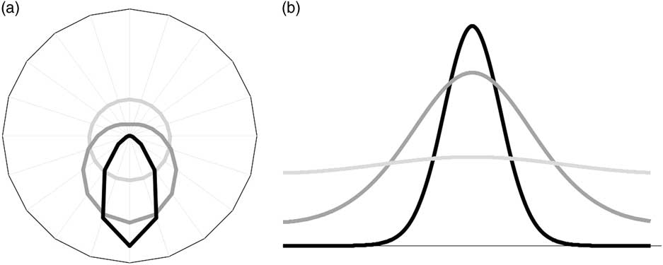
The von Mises distribution (Figure 1) must be viewed as a reasonable assumption for the a priori distribution of y (
 $p\left( {\rm \bf y{\rm \,\mid\,\mu ,\kappa }} \right)$
) because (1) it wraps around a circle, (2) is a close approximation to the circular normal distribution (i.e. it results from wrapping the normal distribution around a unit circle) with the same number of parameters (Breitenberger, Reference Breitenberger1963) and (3) has a more tractable expression, mathematically (Fisher, Reference Fisher1993). Assuming y
i
as the ith circular record, the likelihood of circular data becomes:
 $$p\left( {{\bf{y}}\hskip-2pt\mid\hskip-2pt\mu ,\kappa} \right){\equals}\mathop \prod\limits_{i{\rm {\equals}}1}^n {{e^{{\kappa\,{\rm cos}\left( {y_{i} {\minus}\mu } \right)}} } \over {2\pi \,{\rm I}_{0} \left( \kappa \right)}}$$
where the distribution reduces to a wrapped uniform when κ=0 (Figure 1). It must be noted that κ is a measure of concentration analogous to 1/σ 2 (σ 2 being the variance parameter of the normal distribution), π refers to the ratio of the circumference of a circle to its diameter, and I0(κ) is the modified Bessel function of order 0, that is,
 $$I_{0} \left( \kappa \right){\equals}\mathop \sum\limits_{i{\rm {\equals}}0}^\infty {{\left( {0.{\rm 25}\,\kappa^{2} } \right)^{i} } \over {\left( {{{\it i}\,!\,}} \right)^{2} }}$$
von Mises probability density functions with mean equal to π and dispersion parameter (κ) equal to 0.1 (fair grey line), 1 (dark grey line) and 5 (black line). Plots were presented on a circular (a) and linear (b) parametric space.

Given our current lack of knowledge about circular data, a priori distributions for μ and κ can be stated as uniform between appropriate bounds:
 $$p\left( \mu \right){\equals}{1 \over {{\rm 2}\pi }}({\rm if}\,\mu {\repsilon}[0,2\pi {\rm ]}\,{\rm and}\,0\,{\rm otherwise})$$
 $$p\left( \kappa \right){\equals}{1 \over Y}({\rm if}\,\kappa{\repsilon}{\rm [0,}Y{\rm ]}\,{\rm and}\,0\,{\rm otherwise})$$
where γ is a large enough boundary for κ.
Uncertainly about location parameter
Previous parametrization can generalize to a more flexible hierarchical structure, the CM model. This replaces μ by a set of systematic (b) and random environmental factors (p j ) linked by appropriate incidence matrices (X and Z j ) within an additive structure:
 $${\bf{y}} {\equals}{\bf{Xb}} {\plus}\mathop \sum\limits_{j{\rm {\equals}1}}^r {\bf{Z}} _{j} {\bf{p}} _{j} {\plus}{\bf{e}} $$
Note that e refers to the circular residual term, and flexibility is gained by assuming r independent and normally distributed sources of environmental variation with mean 0 and variance
 $\sigma _{{{\bf{p}} _{j} }}^{2} $
. The joint posterior distribution of all unknown parameters in the model can be obtained from
 $$p\left( {\bf{b}} ,{\bf{p} ,{\bsigma } {\rm ,}\kappa{\rm \,\mid\,}{\bf{y}} } \right)\propto p\left( {{\bf{y}} \,\mid\,{\bf{b}} ,{\bf{p}} {\rm ,}\kappa} \right)p\left( {\bf{b}} \right)p\left( {\bf p\,\mid\,\bsigma } \right)p\left( {\bf \sigma } \right)p\left( \kappa \right)$$
where
 ${\bf p}{\equals}\left[ \bf {p_{1}^{,} p_{2}^{,} \,\ldots\, p_{r}^{,} } \right]^{,} $
and
 ${\bsigma} {\equals}\left[ {\sigma _{{p_{1} }}^{2} \sigma _{{p_{2} }}^{2} \,\ldots\, \sigma _{{p_{r} }}^{2} } \right]$
. As for naive circular (NC) model, the likelihood of data assumes a von Mises process with systematic and permanent environmental sources of variation:
 $${\it p}\left( {{\bf y}\,\mid\,{\bf{b}} ,{\bf{p}} {\rm ,\kappa}} \right){\equals}\mathop \prod\limits_{{\it i{\equals}}\rm 1}^{\it n} {{e^{{{\rm \kappa}{\rm .cos}\left( {{\it y}_{{\it i}} {\minus}\left( {{\bf x}_{{\it i}} {\bf b}{\plus}\sum_{{\it j{\equals}\rm 1}}^{\it r} \nf z_{{{\it i,j}}} {\bf p}_{{\it j}} } \right)} \right)}} } \over {2{\rm \pi I}_{0} \left( {\rm \kappa} \right)}}$$
x i and z i,j being appropriate row vectors of incidence inherent to the ith circular record. Within this context, p must be viewed as a combination of multivariate normal (MVN) processes:
 $${\it p}\left( {{\bf{p}} \,\mid\,{\bf{\bsigma }} } \right){\equals}\mathop \prod\limits_{{\it j{\equals}\rm 1}}^{\it r} {\rm MVN}\left( {\bf 0_{{\it j}} ,{\bf I}_{{\it j}} \sigma _{{{\rm p}_{{\it j}} }}^{2} } \right)$$
where s j is the number of elements in p j , 0 j is a s j × 1 vector of zeros, and I j is a s j × s j identity matrix. Given our current lack of knowledge about systematic effects on the circular parametric space, a priori distributions of b are conceptually defined flat between 0 and 2π:
 $${\it p}\left( {\bf{b}} \right){\equals}{1 \over {{\rm 2\pi }}}({\rm if}\,{\bf{b}} \in\left[ {{\rm 0,2\pi }} \right]{\rm and}\,{\rm 0\hskip3pt otherwise})$$
although an additional restriction applies to guarantee that
 $0\leq {\bf{x}} _{{\it i}} {\bf{b}} {\plus}\mathop \sum\limits_{{\it j{\equals}\rm 1}}^{\it r} {\bf{z}} _{{{\it i,j}}} {\bf{p}} _{{\it j}} \leq {\rm 2\pi }$
. As in previous model:
 $${\it p}\left( {\kappa} \right){\equals}{1 \over {\rm \gamma }}({\rm if}\,{\rm \kappa{\repsilon}}\,{\rm [0,\it Y]\,\rm and}\,0\,{\rm otherwise})$$
whereas
 ${\rm p}\left( {\bf{\sigma }} \right)$
are scaled inverse χ
2 distributions with hyper-parameters ν and S
2 (they become flat when ν=−2 and S
2=0).
Uncertainly about dispersion parameter
Parameter κ in NC and CM models assumes a homogeneous dispersion pattern across all circular data. This assumption may not be true if residual heterogeneity holds in the data set (SanCristobal-Gaudy et al., Reference SanCristobal-Gaudy, Elsen, Bodin and Chevalet1998). Canalization plays a key role in current animal and plant breeding programs to lead more uniform products (Mulder et al., Reference Mulder, Bijma and Hill2008; Blasco et al., Reference Blasco, Martínez-Álvaro, García, Ibáñez-Escriche and Argente2017). Selection for low seasonality in sheep must be viewed as the opposite situation where heterogeneous (i.e. wider) lambing seasons inevitably impacts on other variables such as trade, consumption and lamb prices (Chemineau et al., Reference Chemineau, Malpaux, Brillard and Fostier2007). Generalizing Ibáñez-Escriche et al. (Reference Ibáñez-Escriche, Sorensen, Waagepetersen and Blasco2008), κ can be rewritten as the following hierarchical structure:
 $${\rm \kappa{\equals}}e^{{{\bf{x}} _{i} {{\bbeta }} {\plus}\mathop \sum\limits_{{\it j{\equals}\rm 1}}^r {\bf{z}} _{{{\it i,j}}} {\bf{\brho }} _{{\it j}} }} $$
where β and ρ j have the structure of effects than b and p j , respectively. This expands the Bayesian development to accommodate a circular canalization (CC) model:
 $${\it p}\left( {{\bf{b}} ,{\bf{\bbeta }} ,{\bf{p}} ,{\bf{\brho }} ,{\bf{P}} \,\mid\,{\bf{y}} } \right)\propto{\it p}\left( {{\bf{y}} \,\mid\,{\bf{b}} ,{\bf{\bbeta }} ,{\bf{p}} ,{\bf{\brho }} } \right){\it p}\left( {{\bf{b}} ,{\bf{\bbeta }} } \right){\it p}\left( {{\bf{p}} ,{\bf{\brho }} \,\mid\,{\bf{P}} } \right){\it p}\left( {\bf{P}} \right)$$
where P stores permanent environmental covariances between p and ρ terms (see below). Similarly, the a priori distribution of data includes a hierarchic dispersion term:
 $${\it p}\left( {{\bf{y}} \,\mid\,{\bf{b}} ,{\bf{\bbeta }} ,{\bf{p}} ,{\bf{\brho }} } \right){\equals}\mathop \prod\limits_{{\it i{\equals}}\rm 1}^{\it n} {{{\it e}^{{{\it e}^{{\left( {{\bf x}_{{\it i}} {\bf{\bbeta }} {\plus}\sum_{{\it j{\equals}\rm 1}}^r {\bf{z}} _{{{\it i,j}}} {\bf{\brho }} _{{\it j}} } \right)}} {\rm cos}\left( {{\it y}_{{\it i}} {\minus}\left( {{\bf{x}} _{{\it i}} {\bf{b}} {\plus}\sum_{{\it j{\equals}\rm 1}}^{\it r} {\bf{z}} _{{{\it i,j}}} \rm p_{{\it j}} } \right)} \right)}} } \over {2{\rm \pi I}_{0} \left( {e^{{\left( {{\bf{x}} _{{\it i}} {\bf{\bbeta }} {\plus}\sum_{{\it j{\equals}\rm 1}}^{\it r} {\bf{z}} _{{{\it i,j}}} {\bf{\brho }} _{{\it j}} } \right)}} } \right)}}$$
and the joint distribution of p j and ρ j reduces to a MVN process:
 $${\it p}\left( {{\bf{p}} {\rm ,}{\bf{\brho }} \,\mid\,{\bf{P}} } \right){\equals}\mathop \prod\limits_{{\it j{\equals}\rm 1}}^{\it r} {\rm p}\left( {{\bf{p}} _{{\it j}} ,{\bf{\brho }} _{{\it j}} \,\mid\,{\bf{I}} _{{\it j}} \,\otimes\,{\bf{P}} _{{\it j}} } \right){\equals}\mathop \prod\limits_{{\it j{\equals}\rm 1}}^{\it r} {\rm MVN}\left( {\matrix{ {{\bf{0}} _{{\it j}} } \cr {{\bf{0}} _{{\it j}} } \cr } ,{\rm I}_{{\it j}} \,\otimes\,{\bf{P}} _{{\it j}} } \right)$$
where
 $\,\otimes\,$
is the Kronecker product, and P
j
is the matrix storing permanent environmental variances (
 ${\rm \sigma }_{{{\rm p}_{{\it j}} }}^{2} $
and
 $${\rm \sigma }_{{{\rm \rho }_{{_{{\it j}} }} }}^{2} $$
) and covariances (
 $\sigma _{{p_{j} \rho _{j} }} {\equals}\sigma _{{\rho _{j} p_{j} }} $)
 $${\bf P}_{j} {\equals}\left[ {\matrix{ {\sigma _{{p_{j} }} ^{2} } & {\sigma _{{p_{\it j} \rrho _{\it j} }} } \cr {\sigma _{{p_{j} \rho _{j} }} } & {\sigma _{{\rrho _{j} }} ^{2} } \cr } } \right]$$
Scaled inverse Wishart distributions are used as prior distributions for P j because they enable both scale parameters and covariances to be estimated from data, allow flexibility in the hierarchical model and are computationally convenient (Van Tassell and Van Vleck, Reference Van Tassell and Van Vleck1996).
Markov chain Monte Carlo algorithm
Sampling procedures from the joint posterior distribution will focus on the most complex parametrization (i.e. model CC), as they can be easily adapted to models NC and CM. The algorithm used for posterior sampling was an hybrid approach involving both Metropolis-Hastings (Metropolis et al., Reference Metropolis, Rosenbluth, Rosenbluth, Teller and Teller1953) for b, β, p and ρ, and Gibbs sampling (Gelfand and Smith, Reference Gelfand and Smith1990) for P. Within this context, random samples for systematic (b and β) and permanent environmental effects (p and ρ) where updated from their marginal posterior distribution derived from
 $$\eqalign{{\it p}\left( {{\bf{b}} ,{\bf{\bbeta }} ,{\bf{p}} ,{\bf{\brho }} \,\mid\,{\bf{y}} ,{\bf{P}} } \right) \cr &\hskip -80pt\propto\mathop \prod\limits_{{\it i{\equals}}\rm 1}^{\it n} {{{\it e}^{{{\it e}^{{\left( {{\bf{x}} _{{\it i}} {\bf{\bbeta }} {\plus}\sum_{{\it j{\equals}\rm 1}}^{\it r} {\bf{z}} _{{{\it i,j}}} {\bf{\brho }} _{{\it j}} } \right)}} {\rm cos}\left( {{\rm y}_{{\it i}} {\minus}\left( {{\bf{x}} _{{\it i}} {\bf{b}} {\plus}\sum_{{\it j{\equals}\rm 1}}^{\it r} {\bf{z}} _{{{\it i,j}}} {\bf{p}} _{{\it j}} } \right)} \right)}} } \over {2{\rm \pi I}_{0} \left( {{\it e}^{{\left( {{\bf{x}} _{{\it i}} {\bf{\bbeta }} {\plus}\sum_{{\it j{\equals}\rm 1}}^{\it r} {\bf{z}} _{{{\it i,j}}} {\bf{\brho }} _{j} } \right)}} } \right)}}\cr &\hskip -80pt\mathop \prod\limits_{{\it j{\equals}\rm 1}}^{\it r} {\it e}^{{{\minus}{1 \over 2}\left[{{\bf{p}} _{{\it j}} {\bf{\brho }} _{{\it j}} } \right] ’\lsquo {\bf{P}} _{{\it j}}^{{{\rm {\minus}1}}} \left[ {{\bf{p}} _{{\it j}} {\bf{\brho }} _{{\it j}} } \right]}} $$
For each parameter to be sampled (θ k ), a uniform proposal distribution between between θ k,−1 − π/4 and θ k,−1+π/4 was assumed, where θ k,−1 was the value obtained in the previous iteration. These boundaries were defined in preliminary analyses to guarantee an acceptance rate greater than 10% in all θ k . Once updated for p and ρ, random samples from the marginal posterior distribution of the (co)variance matrix P can be obtained as previously reported by Van Tassell and Van Vleck (Reference Van Tassell and Van Vleck1996) in multivariate linear models.
Example on field data
Lambing distribution throughout the year can be viewed as a representative example of circular quantitative data from livestock industry. This research focused on the re-scaled day of lambing from 1 January (0) to 31 December (regular years, 2π–2π/365; leap years, 2π–2π/366). A total of 110 116 records from 21 630 Ripollesa ewes were collected from 25 purebred flocks between years 1976 and 2017. The Ripollesa is a medium-sized sheep (rams, 75 to 90 kg; ewes, 50 to 65 kg of BW) and the most abundant native ovine breed in Catalonia, the north-east region of Spain. Purebred animals are white with dark brown or black marks on both head and legs, with white semi-fine wool and closed fleece. The Ripollesa breed is a representative example of meat-type sheep management under semi-extensive Mediterranean conditions in northeast Spain, the ‘pascual’-type lamb being its typical commercial product (22 to 24 kg BW at slaughter; Esquivelzeta et al., Reference Esquivelzeta, Fina, Bach, Madruga, Caja, Casellas and Piedrafita2011).
Except for NC parametrization, the analytical model included two systematic and two permanent environmental effects. More specifically, b accounted for ewe age at lambing (<3, 3, 4, 5, 6 and >6 years) and lambing interval (first lambing, <210 days, between 210 and 239 days, between 240 and 329 days, and ⩾330 days); those thresholds balanced the number of records per level, and they had been previously used in this breed for both research and genetic evaluation purposes (Casellas and Caja, Reference Casellas and Caja2014). Permanent environmental effects accounted for flock-year-season with 763 levels, and the environmental contribution of each ewe with 21 630 levels. Although the estimation of the additive genetic merit is the ultimate goal (see companion paper), genetic effects have not been considered in this part. We focus on the fit of the different models and genetic effects should be captured by to the permanent environmental effect inherent to each ewe, if any. Note that flocks were kept under continuous mating systems with multiple sires and paternity testing was not implemented in this breed until 2011; that originated a high percentage of unknown sires in the pedigree file (~95%). Incompleteness of genealogical information discouraged the implementation of animal models under complex genetic covariance structures (Id-Lahoucine and Casellas, Reference Id-Lahoucine and Casellas2017) such as the CC model. If genetic effects are included, fewer ewes with complete pedigree information and close relatives have to be used in order to constrain the estimation problem to a reasonable paradigm. In such a reduced data set, inevitably, the adequacy of each model would be difficult to assess.
All the unknown parameters in models were sampled from their marginal posterior distributions by appropriate Gibbs sampling (Gelfand and Smith, Reference Gelfand and Smith1990) or Metropolis-Hastings (Metropolis et al., Reference Metropolis, Rosenbluth, Rosenbluth, Teller and Teller1953). Three independent Markov chain Monte Carlo (MCMC) with 510 000 iterations were run for each analysis, and the first 10000 iterations were discarded as burn-in. The suitability of the length of the burn-in period was evaluated by both visual inspection and the method of Raftery and Lewis (Reference Raftery and Lewis1992) on the sampling path of κ (NC model) and
 $\sigma _{{{\rm p}_{{\it j}} }}^{2} $
(CM and CC models). A total of 10 000 samples of model parameters were saved from each chain with a lag interval of 50 iterations. All analyses were performed in a server with two Intel® Xeon® E5-2400 (Foxen SA, Madrid, Spain) processors with a CentOS 6.6 Linux operating system. In terms of central processing unit time, the most complex model (CC) spent almost 35 days for each independent 510 000-iteration MCMC.
Model comparison
Model performance was evaluated on two different ways, goodness of fit and predictive ability. Moreover, goodness of fit was assessed twice, by the deviance information criterion (DIC; Spiegelhalter et al., Reference Spiegelhalter, Best, Carlin and van der Linder2002) and the prediction of angular data in terms of mean square error (MSE) between phenotypic and predicted records. The expectation of the predictive distribution of a given ith record (
 $\tilde{y}_{i} $
) under NC model reduced to μ, whereas this expanded to
 ${\bf x}_{{\it i}} {\tilde{\bf b}}_{{\it i}} {\plus}\mathop \sum\limits_{{\it j{\equals}\rm 1}}^{\it r} {\bf z}_{{{\it I,j}}} {\tilde{\bf p}}_{{\it I}} $
under CM and CC models. Note that
 ${\tilde{\bf b}}_{{\it I}} $
and
 ${\tilde{\bf p}}_{{\it I}} $
were posterior modal estimates of b and p
j
. The MSE was calculated in each iteration of the MCMC process as
 $${\rm MSE}{\equals}{{\sum_{{\it i{\equals}\rm 1}}^{\it n} \left( {{\it y}_{{\it i}} {\minus}{\tilde{y}}_{{\it i}} } \right)^{2} } \over {\it n}}$$
On the other hand, predictive ability relied on the prediction of future observations given a trained data sample (Matos et al., Reference Matos, Thomas, Gianola, Pérez-Enciso and Young1997). Two new data sets were created by randomly keeping 50% of records from the initial data set, and both were analyzed under all three models. The MSE was computed for each MCMC iteration between expectations from the predicted distribution and the removed records.
Results and discussion
Phenotypic circular data
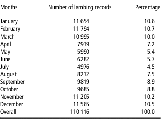
Lambing distribution must be viewed as a worthy example of circular data with relevant implications for the livestock industry (Chemineau et al., Reference Chemineau, Bodin, Migaud, Thiéry and Malpaux2010). The Ripollesa breed concentrated 52.0% of lambing between November and March, whereas the smallest incidence of parturitions was reach in July (4.5%; Table 1). This distribution agreed with the pattern reported in other Mediterranean sheep populations such as several Moroccan (Boujenane, Reference Boujenanet2005), Spanish (García-Pérez et al., Reference García-Pérez, Hurtado, Oregui and Juste2002), Italian (Finocchiaro et al., Reference Finocchiaro, van Kaam, Portolano and Misztal2005) and Greek breeds (Avdi et al., Reference Avdi, Driancourt and Chemineau1993). Although these Mediterranean breeds were suggested as moderately seasonal in terms of reproductive performance, they still show a remarkable winter-spring lambing season under continuous mating systems.
Distribution of Ripollesa sheep lambing data per month

The estimated circular mean in the Ripollesa breed was 0.622 radians or, alternatively, 5 February on a calendar basis. On the other hand, the variance as defined by Fisher (Reference Fisher1993) was 0.815. It is important to note that a value near 0 implies that there is little variation in values of the angles, and a value of 1 highlights maximum variation (i.e. uniform distribution). Within this context, lambing distribution in the Ripollesa breed showed a moderate-to-high variability as well as an uni-modal distribution as noted in Table 1. This revealed this data set as an appealing starting point to test the different sources of variation on the circular parametric space under the different models developed above.
Goodness-of-fit
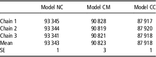
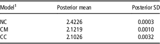
Goodness-of-fit in the Ripollesa data set has been evaluated by the DIC (Table 2) and the MSE (Table 3). The DIC statistic evaluates both model fit and complexity. Smaller DIC values indicate a better model fit and lesser degree of complexity and, in general, differences between models larger than 3 to 5 DIC units are assumed as statistically relevant (Spiegelhalter et al., Reference Spiegelhalter, Best, Carlin and van der Linder2002). Regarding lambing distribution, the NC model reached the worse fit with an average DIC of 93 343 units. On the other hand, CM and CC models reduced the average DIC in 2520 and 5425 units, respectively. A similar pattern was evidenced by the MSE. The worse fit was reached by the NC model (2.4226 radiants2), whereas CM and CC models reduced MSE in 12.4% and 13.2%, respectively. Moreover, 95% highest posterior density of MSE under CM and CC models did not overlap (results not shown).
Deviance information criterion (Spiegelhalter et al., Reference Spiegelhalter, Best, Carlin and van der Linder2002) for lambing distribution in the Ripollesa sheep breed under naive circular (NC), circular mixed (CM) and circular canalization (CC) model

Estimates where provided for each of the three independent Monte Carlo Markov chains.
Goodness-of-fit of circular models in terms of mean square error between observed and predicted records for lambing distribution in the Ripollesa sheep breed

1 Naive circular (NC) model, circular mixed (CM) model and circular canalization (CC) model.
These are the first available results comparing goodness-of-fit of different circular parametrizations for the analysis of lambing distribution. Although there are not comparable results within the context of circular models, the poor fit obtained under NC model could be anticipated. This parametrization was included as a mere introduction to the analysis of circular data under a Bayesian context, although this becomes useful to set the starting point for CM and CC models. On the other hand, the under-performance of model NC highlighted the relevance of systematic and/or permanent sources of variation included in the two competing models, as previously suggested by other authors (Gündoğan et al., Reference Gündoğan, Baki and Yeni2003; Rosa and Bryant, Reference Rosa and Bryant2003; Chemineau et al., Reference Chemineau, Bodin, Migaud, Thiéry and Malpaux2010).
Differences between CM and CC models were remarkable both in terms of DIC and MSE. Although heteroskedasticity had not been previously evaluated on circular data from the livestock industry, this phenomenon was already revealed on multiple linear traits from domestic species (Gutiérrez et al., Reference Gutiérrez, Nieto, Piqueras, Ibáñez-Escriche and Salgado2006; Marjanovic et al., Reference Marjanovic, Mulder, Khaw and Bijma2016). Permanent and systematic effects contributed statistically relevant departures in the circular variability of lambing distribution, improving the goodness-of-fit of the model when they were properly accounted for. Moreover, these sources of variation must be viewed as potential tools to reduce seasonality in the meat-type sheep industry (by increasing variance of lambing distribution) and allow a year-round lamb production. Although these results cannot be directly extrapolated to all circular traits, the potential impact of canalization models must be taken into account.
Predictive ability
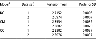
The MSE for the different circular models used to predict the removed lambing data records in the Ripollesa data set are shown in Table 4. Estimated MSE were greater than for the goodness-of-fit analyses, which was not surprising because analyses were performed with fewer records and the ones involved in the calculation of MSE did not contribute information to the analysis itself. This behavior for predictive ability has been previously reported in other studies focused on linear or threshold models (Matos et al., Reference Matos, Thomas, Gianola, Pérez-Enciso and Young1997; Varona et al., Reference Varona, Misztal and Bertrand1999). As for goodness-of-fit, the CC model reached the smallest MSE values, with a moderate advantage in front of CM model, although larger than in Table 3, and huge differences with NC model (Table 4). Within this context, heteroscedacity must be viewed as a real phenomenon influencing lambing distribution in the Ripollesa sheep breed. Moreover, random sources of variation in CC parametrization had crossed dependencies between location and variance parameters (i.e. p j and ρ j ) through a covariance term. As previously suggested in bivariate models (Varona et al., Reference Varona, Misztal and Bertrand1999), the heteroskedastic term may be a useful source of addition information to substantially improve predicted ability of the canalization model.
Predictive ability of circular models in terms of mean squared error between the observed and predicted records of lambing distribution in the Ripollesa sheep breed

Note that two data sets were created by removing 50% of the records and mean square error was computed between expectations from the predicted distribution and the removed records.
1 Naive circular (NC) model, circular mixed (CM) model and circular canalization (CC) model.
2 Two new data sets were created with 50% of records removed from each (data sets 1 and 2).
Circular mixed models in the livestock industry
The results presented here suggested that the von Mises mixed model was well suited to account for the analysis of lambing distribution, this being able to account for different sources of variation in the centrality and the dispersion term. The choice of the von Mises model must be viewed as a reasonable compromise between mathematical convenience and biological plausibility, providing a more realistic framework than linear models (Knight et al., Reference Knight, Dalton and Hight1980). Moreover, this approach can be applied to multiple data sources from the livestock industry such as meat color analyses (Girolami et al., Reference Girolami, Napolitano, Faraone and Braghieri2013), cardinal tracks (Begall et al., Reference Begall, Červený, Neef, Vojtěch and Burda2008; Schiffner et al., Reference Schiffner, Siegmund and Wiltschko2014) or other time-related biological rhythms such as estrus detection on a 24-h basis in cows (Xu et al., Reference Xu, McKnight, Vishwanath, Pitt and Burton1998), or oviposition time in broilers (Lewis et al., Reference Lewis, Backhouse and Gous2004), among others.
Finally, CM and CC models can be extended to include infinitesimal additive genetic effects (i.e. breeding values) in order to predict the genetic predisposition to advance or postpone the lambing season (uncertainly about the location term), or to accentuate or attenuate seasonality (uncertainly about the dispersion term). It is important to highlight that although the von Mises assumption was found satisfactory for systematic and permanent environmental effects, nothing guarantees that this is still the case for additive genetic effects when added to CM and CC models. The validity of this assumption will require further investigation in the companion paper.
Acknowledgements
The authors are indebted to the Ripollesa breed society for contributing field data. M.M.d.H.-V. was supported by a scholarship (BES-2017-080596) from the Ministerio de Economía, Industria y Competitividad of Spain’s government (Madrid, Spain).
Declaration of interest
The authors do not have conflicts of interest with the subject matter of this manuscript.
Ethics statement
Animal Care and Use Committee approval was not necessary for this study because analyses were performed on existing field data obtained under standard farm management from commercial breeders. Both productive and reproductive data were collected by the stockbreeders themselves and administrated by the Ripollesa Breed Society (Associació Nacional de Criadors d’Oví de Raça Ripollesa (ANCRI), Monells, Spain) within the context of its yield recording program.
Software and data repository resources
Data and model used for the purpose of this study are not deposited in an official repository.