1 Introduction
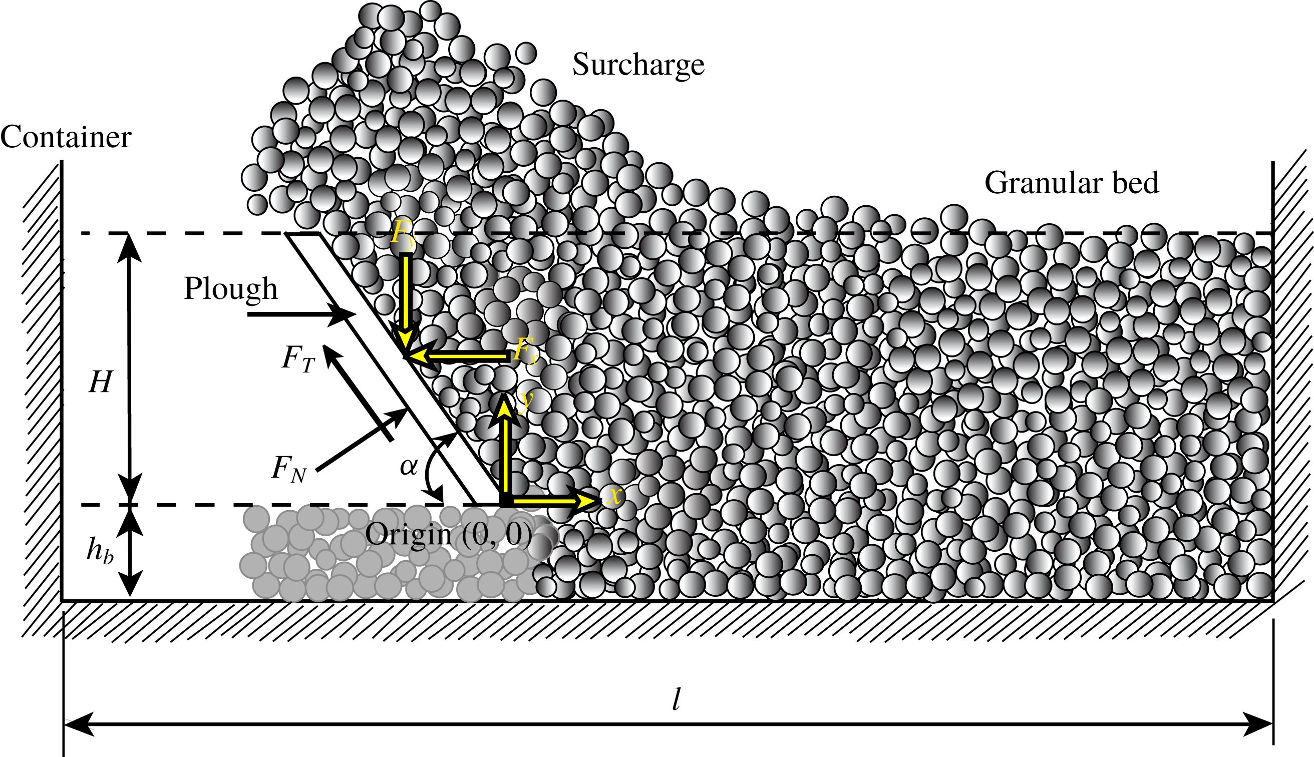
Ploughing or excavation (figure 1) is an important process that finds application in industries like agriculture, mining, construction and earth-moving. Modelling such processes is challenging because of the complex nonlinear behaviour of granular material, its spatial variability and the dynamic effects that may occur during rapid granular flow. Ploughing is a power-intensive process and the prediction of forces on the plough is essential for better machine design. At the same time, estimating forces on fully or partially submerged objects moving relative to a granular medium remains a problem of fundamental importance; see, e.g. Wieghardt (Reference Wieghardt1975), Bharadwaj, Wassgren & Zenit (Reference Bharadwaj, Wassgren and Zenit2006), Seguin et al. (Reference Seguin, Bertho, Gondret and Crassous2011) and Katsuragi & Durian (Reference Katsuragi and Durian2013).
Various methods have been developed in the past to study the ploughing process. Analytical methods are based on Terzaghi’s passive soil pressure theory (Hettiaratchi, Witney & Reece Reference Hettiaratchi, Witney and Reece1966; McKyes & Ali Reference McKyes and Ali1977). These methods model the failure pattern in granular media and take the process to be quasi-static. Sokolovski (Reference Sokolovski1960) employed slip-line theory, which assumes that failure inside the bulk occurs at certain planes. In these methods complicated plough geometries and dynamic effects cannot be taken into account. Furthermore, slip-line theory is limited to two dimensions and to rigid perfectly plastic materials. At the same time, analytical methods developed for three dimensions (Hettiaratchi & Reece Reference Hettiaratchi and Reece1967) make many simplifying assumptions and are restricted to quasi-static processes. Recently Gravish, Umbanhowar & Goldman (Reference Gravish, Umbanhowar and Goldman2010) fitted their experimental results about forces in ploughed grains through the method of wedges (Nedderman Reference Nedderman1992), which is a quasi-static technique. Finally, we mention the work of Palmer (Reference Palmer1999) and Sauret et al. (Reference Sauret, Balmforth, Caulfield and McElwaine2014). Sauret et al. (Reference Sauret, Balmforth, Caulfield and McElwaine2014) investigated bulldozing of granular material through experiments and continuum depth-averaging techniques, but did not compute the forces exerted by the granular flow on the plough. Palmer (Reference Palmer1999) explored the effect of speed during rapid cutting of water-saturated soils. An analytical model is developed for the change in pore pressure, and the increase in cutting effort is explained through a drop in pore pressure which augments effective stresses. Models/techniques to predict the cutting forces are not developed. In contrast, our work concerns dry granular materials, and we put forward a methodology to estimate forces during cutting (ploughing).
Schematic of ploughing, where a flat, rigid, inclined plough moves through a granular bed. The coordinate system
 $(x{-}y)$
in which we will work is attached to the plough’s tip. The inclination angle of the plough is
 $\unicode[STIX]{x1D6FC}$
,
 $H$
is the depth of the plough in the granular bed measured from the undisturbed bed’s surface,
 $h_{b}$
is the distance of the plough’s tip from the base of the container and
 $l$
is the length of the container. The plough moves to the right at speed
 $v_{c}$
. The force acting on the plough may be split along and normal to the plough as, respectively,
 $F_{N}$
and
 $F_{T}$
, or along the given
 $(x{-}y)$
coordinate system as
 $F_{x}$
and
 $F_{y}$
, respectively. In the main text we will typically compute
 $F_{x}$
and
 $F_{y}$
.

Ploughing involves large deformations during which grains may lose or come into contact. Because of this, it becomes difficult to model ploughing of a granular bed through finite element methods. Most current studies employ the discrete element (DE) method, developed by Cundall & Strack (Reference Cundall and Strack1979), or its extensions. Examples of application of the DE method to processes like ploughing and soil cutting include Ono et al. (Reference Ono, Nakashima, Shimizu, Miyasaka and Ohdoi2013), who studied soil cutting resistance using three-dimensional DE simulations, Asaf, Rubinstein & Shmulevich (Reference Asaf, Rubinstein and Shmulevich2007), who analysed cutting blade shapes using two-dimensional DE simulations, and Coetzee (Reference Coetzee2014), who compared the efficacy of DE and continuum (material point) methods in modelling soil cutting. The experiments of Percier et al. (Reference Percier, Manneville, McElwaine, Morris and Taberlet2011) and Guo et al. (Reference Guo, Goldsmith, Delacruz, Tao, Luo and Koehler2012) on forces experienced during ploughing were also explained using two-dimensional DE simulations. Guo et al. (Reference Guo, Goldsmith, Delacruz, Tao, Luo and Koehler2012), additionally, employed an extended Coulomb’s Earth pressure theory (Nedderman Reference Nedderman1992) to model their observations. This was consistent because Guo et al. (Reference Guo, Goldsmith, Delacruz, Tao, Luo and Koehler2012) ploughed at very slow rates.
Gravish, Umbanhowar & Goldman (Reference Gravish, Umbanhowar and Goldman2014) recently utilized resistive force theory (RFT) to estimate forces during ploughing. This technique was initially developed for computing the drag on intruders in viscous fluids, and then later extended to intruders in granular media (Li et al. Reference Li, Umbanhowar, Komsuoglu, Koditschek and Goldman2009; Ding, Gravish & Goldman Reference Ding, Gravish and Goldman2011). In RFT, the total load on an intruder is found by dividing the intruder into smaller elements, computing the loads on these elements separately either through experiments or simulations, and then assuming that the total load on the intruder is the sum of the loads on all its elements. Thus, a fundamental assumption is that the loads experienced by an element of the intruder are unaffected by the presence of the rest of the intruder (Aguilar et al. Reference Aguilar, Zhang, Qian, Kingsbury, McInroe, Mazouchova, Li, Maladen, Gong and Travers2016; Askari & Kamrin Reference Askari and Kamrin2016; Slonaker et al. Reference Slonaker, Motley, Zhang, Townsend, Senatore, Iagnemma and Kamrin2017). Even in isolation, the force per unit area acting on each intruder element depends upon its orientation and velocity, and the flow velocity of the grains. At the same time, as part of the intruder, the orientation and velocity of an element, and the flow’s local velocity will vary, and may even change. Thus, the force on an isolated intruder element for a range of velocities and orientations has to be found, and then superposed to find the total load on the intruder. A complete physical and mathematical explanation of why superposition of forces employed in RFT succeeds in nonlinear systems like granular flows is unavailable, although Askari & Kamrin (Reference Askari and Kamrin2016) have attempted to provide necessary conditions to predict the materials wherein RFT may work. We list the main differences between RFT and our approach in § 2.
A central challenge in applying the DE method directly to granular flows is the calibration of the grain micro-properties. This is necessary to ensure that the virtual (i.e. simulated) granular material displays the macroscopic constitutive response of the grains being investigated. Parameters entering the interaction law governing grain-to-grain contact in the DE simulations are determined using theory, trial-and-error or experiments. Coetzee (Reference Coetzee2017) reviews the many calibration procedures employed by various researchers. For example, Tanaka et al. (Reference Tanaka, Momozu, Oida and Yamazaki2000) compared the results of DE simulations with actual bar penetration tests. They varied the friction coefficient between grains to determine the value that provided the best comparison. Shmulevich, Asaf & Rubinstein (Reference Shmulevich, Asaf and Rubinstein2007) found interaction parameters from in situ field tests. They compared their test results and simulations and applied a nonlinear optimization algorithm to locate optimal grain parameters for use in simulations. Coetzee & Els (Reference Coetzee and Els2009) employed a combination of shear tests and compressions tests of grains simulated through the DE method, and compared these results with experimentally measured friction angle and stiffness to determine the best set of grain friction and grain stiffness values. Thus, calibration (i) requires significant effort, (ii) is often application specific and (iii) is not standardized.
Even after the grain parameters have been calibrated for an application, in order to obtain accurate and robust force data with low noise, it is found necessary to employ a very large number of grains. For example, Tsuji et al. (Reference Tsuji, Nakagawa, Matsumoto, Kadono, Takayama and Tanaka2012) employed 300 000 grains in their simulation of bulldozing. Sometimes even grain shapes have to be modelled more exactly than as mere spheres; for example, Coetzee & Els (Reference Coetzee and Els2009) employed clumped spherical grains to model the shape of corn grains used in their experiments. These aspects significantly increase the computational cost.
Here, we propose to obtain forces during ploughing by combining kinematic data obtained from coarse, but representative, DE simulations with continuum mechanics. This approach circumvents the necessity of extensive calibration of DE simulations, and also does not require a very large number or complex shapes of grains. Computational cost is, thus, significantly lowered and, at the same time, greater insight is obtained into which kinematic aspects of the flow affect its kinetics the most. We identify our approach as the extended strain path method (ESPM), as its spirit is somewhat similar to the strain path method developed by Baligh (Reference Baligh1985) for deep, quasi-static penetration processes. The main differences (and advantages) being that ESPM is applicable to dynamic processes, and may be applied to those granular flows in which strain paths are not easily visualized in experiments. We develop and demonstrate ESPM in the context of two-dimensional ploughing. Additionally, we employ a simple rheology for the granular flow, in order to keep the number of fitted parameters to a minimum. The method may, however, be extended to three dimensions and more complex rheologies.
Computing the continuum velocity field of the flowing grains is a fundamental step in ESPM. Deformation fields for applications similar to ours have been studied in the past using various techniques, and we briefly summarize them. Wettergreen et al. (Reference Wettergreen, Moreland, Skonieczny, Jonak, Kohanbash and Teza2010) and Loret de Mola Lemus et al. (Reference Loret de Mola Lemus, Kohanbash, Moreland and Wettergreen2014) investigated the motion of a rover on sand and controlled it by actuating a plough. The force on the plough required for braking is measured in terms of wheel slip. Moreland et al. (Reference Moreland, Skonieczny, Inotsume and Wettergreen2012) visualized the complex soil flow patterns under a wheel using a shear interface imaging analysis tool. The deformation fields obtained were for soil–wheel interaction, and are not directly relevant to our case.
Murthy, Gnanamanickam & Chandrasekar (Reference Murthy, Gnanamanickam and Chandrasekar2012) and Yadav, Saldana & Murthy (Reference Yadav, Saldana and Murthy2015) obtained deformation fields during indentation of a granular bed in a rectangular chamber. It is important to note that, because metals can withstand significant tensile forces while, in contrast, granular materials have almost no tensile strength, many of the features observed in metals, especially at the surface, may not be found in grains. Finally, Murthy et al. (Reference Murthy, Saldana, Yadav and Du2013) performed soil cutting experiments with a vertical plough, and generated velocity contour maps using image analysis; these, as we will see in § 4.1, resemble what we find in simulations.
In passing we mention some recent techniques that have been employed to measure the large deformation inherent in granular materials. These include fine grid techniques (Sevenhuijsen, Sirkis & Bremand Reference Sevenhuijsen, Sirkis and Bremand1993; Goldrein, Palmer & Huntley Reference Goldrein, Palmer and Huntley1995), which analyse images of distorted surface grids to produce quantitative displacement and strain maps, and digital speckle X-ray flash photography (Goldrein et al. Reference Goldrein, Grantham, Proud and Field2002; Grantham et al. Reference Grantham, Proud, Goldrein and Field2006), which combines digital speckle photography with flash X-ray photography to measure two- and three-dimensional displacement fields within bodies undergoing dynamical deformation.
Finally, we mention the work of Qiong, Pitt & Ruina (Reference Qiong, Pitt and Ruina1986) who found forces exerted by soil on a plough mouldboard by constructing strain paths from scratch traces left on the mouldboard. In this, they too followed a strain path method. However, assumptions about the flow that they made, while perfectly suitable for a mouldboard, are not easily extended to other flows, such as the one investigated here.
The rest of the paper is organized as follows. We discuss ESPM in the next section. Our DE simulations, from which we obtain kinematic data, are described in § 3. We then obtain the continuum strain rate field in § 4 by homogenizing the position data computed from DE simulations. Next, we test the extent of the applicability of ESPM by probing the degree to which ploughing is kinematically controlled. We then introduce a continuum model of the granular flow in § 5 and combine it with the strain rates obtained from DE simulations and linear momentum balance to calculate stresses in the bulk. This, subsequently, allows us to estimate forces on the plough. Finally, in § 6 we present our results. We observe a good match between our ESPM predictions and calibrated DE simulations, and also with experiments conducted by us and others.
2 Extended strain path method
The ESPM combines DE simulations and continuum analysis and has the following main steps.
- Step 1:
Obtain an approximation to the strain rate field, while modelling the granular material as a continuum. This may be done through experiments, e.g. Baligh (Reference Baligh1985) or Qiong et al. (Reference Qiong, Pitt and Ruina1986), or simulations, as we propose. Here, we employ representative DE simulations that are fairly coarse and do not employ calibrated grain properties. Hence, the total computational effort is much lower than purely computational paradigms (e.g. Coetzee Reference Coetzee2014).
- Step 2:
Select an appropriate continuum constitutive description of the flowing grains. We will model the granular material as a pressure-dependent Bingham fluid (Sharma Reference Sharma2017, § 2.10.1), which is very similar to the
 $\unicode[STIX]{x1D707}(I)$
-rheology proposed by Jop, Forterre & Pouliquen (Reference Jop, Forterre and Pouliquen2006). A Bingham fluid (Oldroyd Reference Oldroyd1947; Prager Reference Prager1961, p. 136) has the property that it remains rigid until the stresses violate a yield criterion, after which it flows. The yield criterion may or may not be pressure-dependent, and we employ a pressure-dependent yield criterion to match with observed behaviour in granular materials. We employ a simple rheology in order to minimize the number of fitted parameters.
- Step 3:
Combine the strain field of step 1 with the constitutive description of step 2 and linear momentum balance to obtain the stress field in the granular material being ploughed. From this the forces acting on the plough may be estimated.

Implicit in this approach is the assumption that deformations during ploughing are greatly constrained by the system’s geometry, to the extent that the strain rate field does not vary significantly for media containing grains with different properties, e.g. size, shape, texture, density, inelasticity. Thus, the strain rate field may be estimated fairly accurately without matching the actual properties of the grains in the material being ploughed. We will test the validity of this assumption by performing DE simulations with several different choices of grain parameters: friction coefficients, grain sizes and polydispersities. At the same time, we emphasize that our ultimate aim is to predict the forces on the plough and not the strain field. Thus, variations in the strain rates that appear significant from a kinematic viewpoint may, in fact, not be that consequential to the kinetics.
Our approach above is somewhat similar to the strain path method developed by Baligh (Reference Baligh1985) for geotechnical problems, specifically deep penetration problems. Similar kinematic-based analyses that utilize hydrodynamic models have been developed for modelling high-velocity impacts into metals (see, e.g. Birkhoff et al. Reference Birkhoff, MacDougall, Pugh and Taylor1948; Alekseevskii Reference Alekseevskii1966; Tate Reference Tate1967, Reference Tate1969, Reference Tate1978, Reference Tate1986a ,Reference Tate b ; Yarin, Rubin & Roisman Reference Yarin, Rubin and Roisman1995; Rubin Reference Rubin2012; Sharma Reference Sharma2019). Baligh (Reference Baligh1985) guessed or estimated the strain field from penetration experiments in saturated clays. In contrast, the strain field for ploughed grains has not been reported. In our approach, we obtain kinematic information from representative, but coarse and uncalibrated, DE simulations. We therefore identify our approach as an ESPM. The advantage is that, with DE simulations, we are able to visualize the kinematics of granular flows in complex and/or three-dimensional geometries that may be inaccessible to experiments. Furthermore, ESPM may be utilized in dynamic processes where inertia plays a role. These features will allow application of ESPM to many more processes.
Finally, we list the main differences between RFT (Gravish et al. Reference Gravish, Umbanhowar and Goldman2014) and ESPM:
(i) RFT estimates forces on intruders in granular flows, while ESPM may also be employed for flows across infinite surfaces.
(ii) RFT does not describe the flow and stress fields in the granular media, while ESPM can estimate them.
(iii) ESPM finds the flow kinematics from coarse DE simulations without a great need for matching grain parameters in the DE simulations (cf. § 4.3). Thus, one DE simulation provides all kinematic information necessary for flows of different types of grains, but the same system geometry. The constitutive law accounts for the difference in grain types. In contrast, RFT requires multiple experiments/simulations to map out forces at all orientations and velocities of an intruder element, which will have to be repeated when the grain type is changed. Li, Zhang & Goldman (Reference Li, Zhang and Goldman2013) suggest that information for different orientations and grain types could be obtained by scaling/fitting laws for flat-faced planar elements. However, the accuracy and efficacy of these fits have not yet been documented comprehensively.
(iv) In ESPM, the effort required to simulate flows over complex geometries (e.g. curved ploughs) is comparable to that of simpler shapes like flat-faced ploughs. In contrast, RFT may entail a larger number of experiments/simulations. It is also possible that planar elements may not work for more complicated shapes. To that extent, ESPM may be easier to implement for complex geometries.
(v) Finally, it is unclear how RFT will work in transient problems. In contrast, ESPM can be extended to transient problems by utilizing transient DE simulations.
We will now apply ESPM to find the forces required during ploughing of a granular bed in two dimensions. We will begin by describing our DE simulations that are required in step 1 above.
3 Simulation methodology
3.1 Geometry
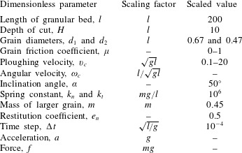
Figure 1 shows a schematic of a typical two-dimensional ploughing operation with a flat, rigid, inclined plough. To set up our DE simulations, first a bed of grains is prepared by dropping grains in a rectangular container freely under gravity. The container has a length of 200 non-dimensional units. Table 1 lists relevant non-dimensional parameters. To prevent lattice formation, equal amounts of two differently sized grains with diameters in the ratio of 1:0.7 were taken. This ensures a spatially random distribution of grains. Bhateja, Sharma & Singh (Reference Bhateja, Sharma and Singh2016, Reference Bhateja, Sharma and Singh2017) provides details of our DE simulations. The plough is also made up of disc-shaped grains with half the diameter of the larger grains; see inset in figure 3. This method of modelling the plough allows us to readily model any shape of plough.
Once the bed is prepared, the plough moves from the left to the right at a constant velocity. We note from figure 1 that the rectangular container has a wall at its right end. This is required to define the computational domain. This wall does not affect the flow until it is less than
 $70$
non-dimensional units away from the plough’s tip. As shown in figure 2, the flow of grains is steady when the plough travels between
 $50$
and
 $130$
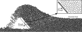
non-dimensional units from the left-hand side wall (see caption). Figure 3 shows a snapshot from the DE simulation of the flow at steady state.
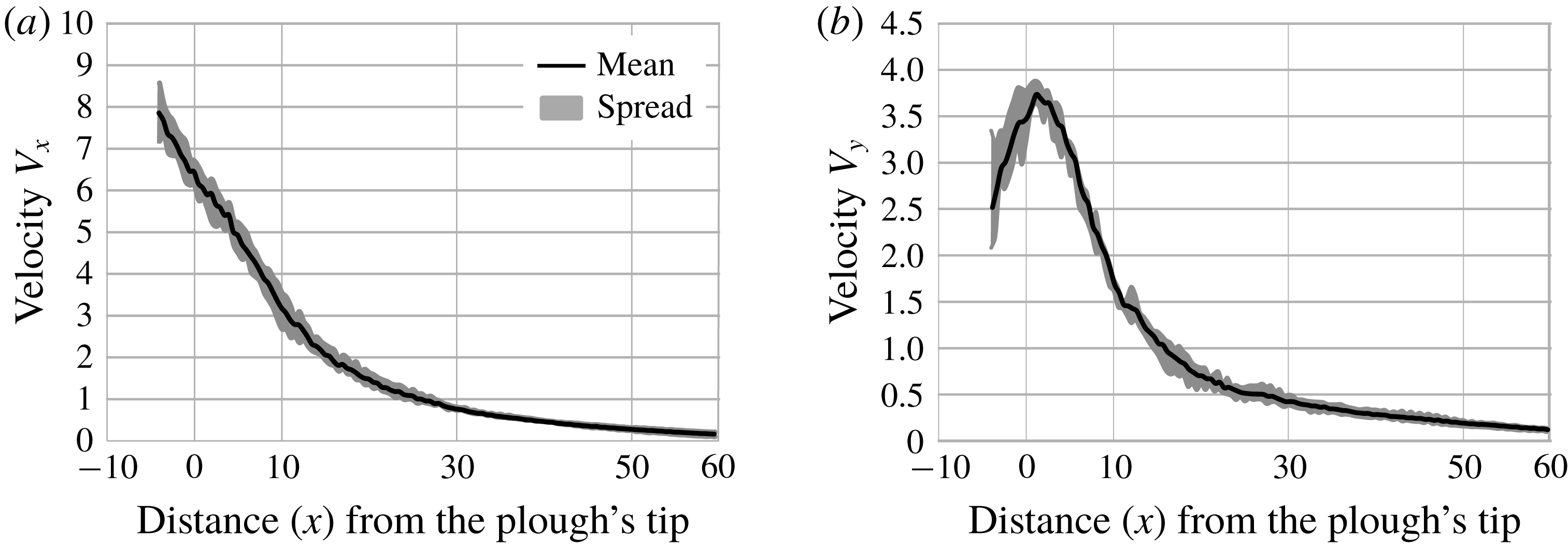
The continuum velocity field associated with the granular material, calculated as per § 4.1, is plotted at points along the line
 $y=9$
. The velocity field was computed at five time instants during the time in which the plough’s tip moves from
 $x=50$
to 130, which corresponds to a distance of 150 to 70 non-dimensional units away from the right-hand boundary. The mean of these five samples (black curve) and the spread about the mean (grey region) are shown. (a) Velocity
 $V_{x}$
along
 $x$
. (b) Velocity
 $V_{y}$
along
 $y$
. The plough’s non-dimensional speed
 $v_{c}=10$
, the inter-grain friction
 $\unicode[STIX]{x1D707}=0.3$
and grain diameter
 $d=0.67$
.

Finally, we note that in simulations it is possible to both allow or restrict rotation of the grains. We compare outcomes from the two in § 4.3.1 and show that both choices provide essentially the same strain rate fields. Subsequently, we only utilize simulations wherein grain rotations are restricted.
Snapshot from a DE simulation. The inset shows details of how the plough is modelled. We modelled the plough by arranging plough-grains in a straight line close to each other. The size of these grains compared to that of flowing grains defines the smoothness of the plough’s surface. Rearranging the grains to follow a defined trajectory would allow us to readily model any shape of plough.

Dimensionless parameters employed in simulations.

4 Kinematics
All computations are done in a coordinate system attached to the plough’s tip, as shown in figure 1. Unit vectors
 $\hat{\boldsymbol{i}}$
and
 $\hat{\boldsymbol{j}}$
point along
 $x$
and
 $y$
directions, respectively.
4.1 Continuum velocity field
Our ESPM requires the continuum velocity field
 $\boldsymbol{V}$
to obtain strain rates. From DE simulations we obtain position data for each grain at every time step. Velocities of grains are calculated by noting displacements at short time intervals and dividing them by the time interval. The time interval is chosen small enough so as to restrict displacement to less than one grain diameter. The position of a grain is taken to be the mean of the positions at the beginning and at the end of the time interval. Thus, if
 $\boldsymbol{r}_{p}^{n}$
and
 $\boldsymbol{r}_{p}^{n+1}$
are the positions of the
 $p$
th grain at times
 $t^{n}$
and
 $t^{n+1}$
, respectively, then we define the grain velocity
 $$\begin{eqnarray}\boldsymbol{U}(\boldsymbol{r}_{n+1/2},t_{n+1/2})=\frac{\boldsymbol{r}_{p}^{n+1}-\boldsymbol{r}_{p}^{n}}{t^{n+1}-t^{n}},\quad \text{where}~\{\boldsymbol{r}_{n+1/2},t_{n+1/2}\}=\left\{\frac{\boldsymbol{r}_{p}^{n}+\boldsymbol{r}_{p}^{n+1}}{2},\frac{t^{n}+t^{n+1}}{2}\right\}.\end{eqnarray}$$
Thus, the velocity of each grain is obtained as a function of position at different time steps. The flowing grains are now thought to constitute a continuum. We next extract a continuum velocity field from
 $\boldsymbol{U}(\boldsymbol{r}_{n+1/2},t_{n+1/2})$
.
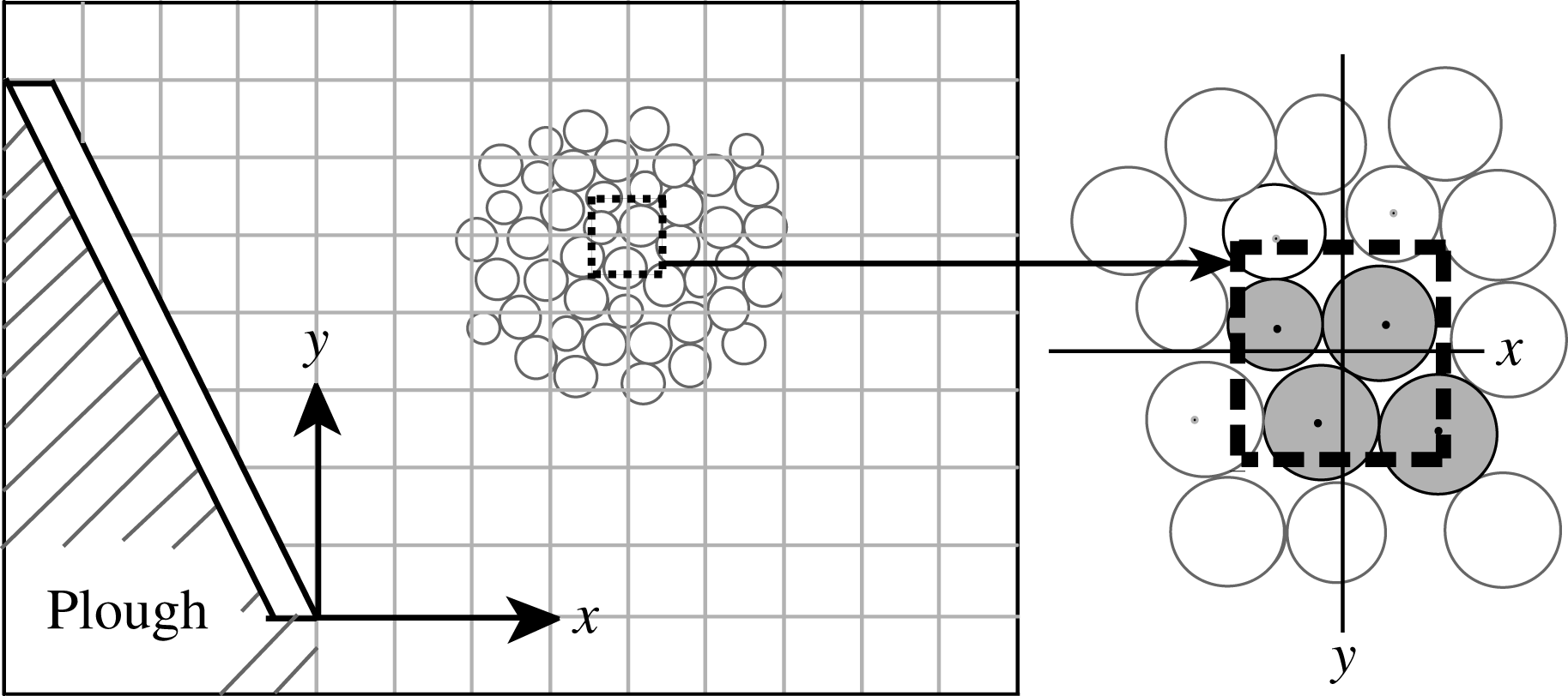
Schematic of the square grid employed to post-process data obtained from DE simulations. The inset shows a square (dashed lines) of size
 $0.5\times 0.5$
constructed around the grid point
 $(x,y)$
. The velocities of all shaded grains, whose centres lie within the square, are averaged, and the resultant velocity is assigned to the grid point
 $(x,y)$
. Grains lying in hatched region are not relevant to our computations and are, therefore, ignored. Figure is not to scale.

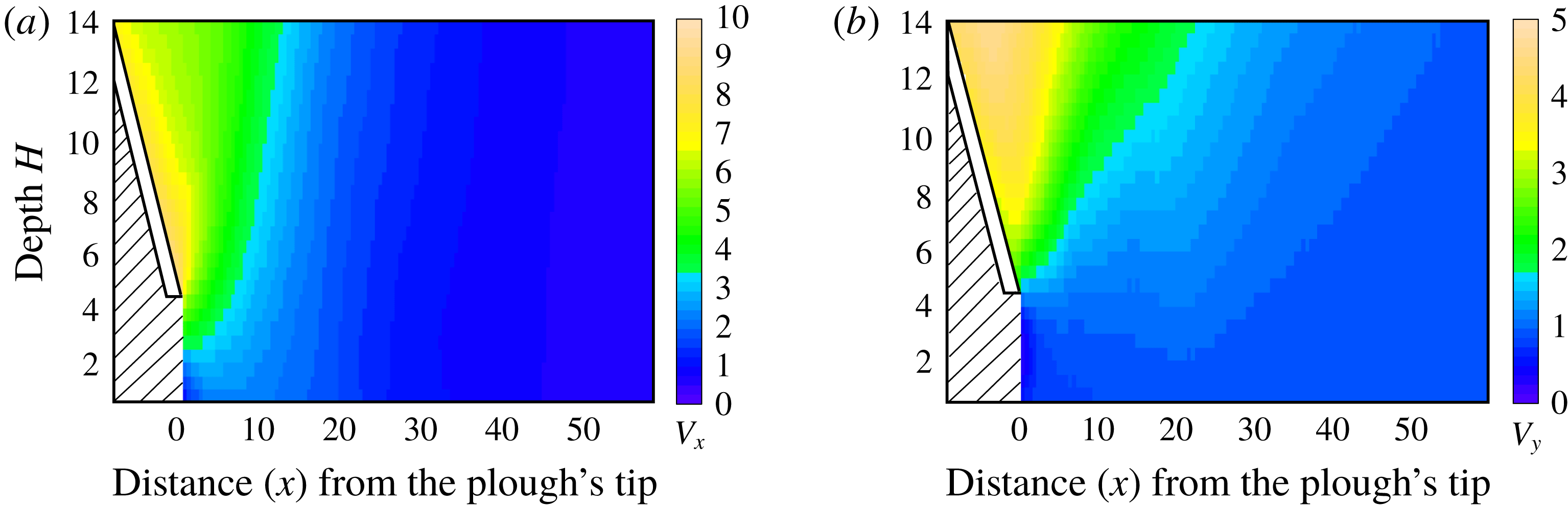
Continuum velocity field associated with the granular material for a plough moving with non-dimensional speed
 $v_{c}=10$
. (a) Horizontal velocity component
 $V_{x}$
. (b) Vertical velocity component
 $V_{y}$
. We do not report information in the hatched area.

A fixed square grid with a grid size of
 $0.5$
non-dimensional units is constructed covering the region of interest; see figure 4. The continuum’s velocity field
 $\boldsymbol{V}(x,y,t)$
at any time
 $t$
is obtained at a point
 $(x,y)$
of this grid by averaging the velocities
 $\boldsymbol{U}$
of the grains whose centres lie within the square grid, as demonstrated in figure 4. Once the velocity field is known, the acceleration may be calculated through
 $$\begin{eqnarray}\boldsymbol{a}=\frac{\unicode[STIX]{x2202}\boldsymbol{V}}{\unicode[STIX]{x2202}t}+\unicode[STIX]{x1D735}\boldsymbol{V}\boldsymbol{\cdot }\boldsymbol{V}.\end{eqnarray}$$
The continuum velocity field
 $\boldsymbol{V}$
thus obtained at different time instants is noisy due to inherent fluctuations of the flowing grains. In a steady flow, we average the velocity field data over time to reduce randomness. In a developing flow, the transient time range is divided into finite time windows, over which time averaging is then performed. We have seen that the size of the time window should, at least, be equal to the time it takes the plough to cover a distance of 15 grain diameters in order to remove the randomness in the velocities. An example of a computed velocity field is shown in figure 5. The velocity field that we compute resembles that found by Murthy et al. (Reference Murthy, Saldana, Yadav and Du2013, figure 3) in their preliminary experiments on a vertical plough.
Henceforth, we will work with the continuum velocity field
 $\boldsymbol{V}$
rather than with the velocity of individual grains.
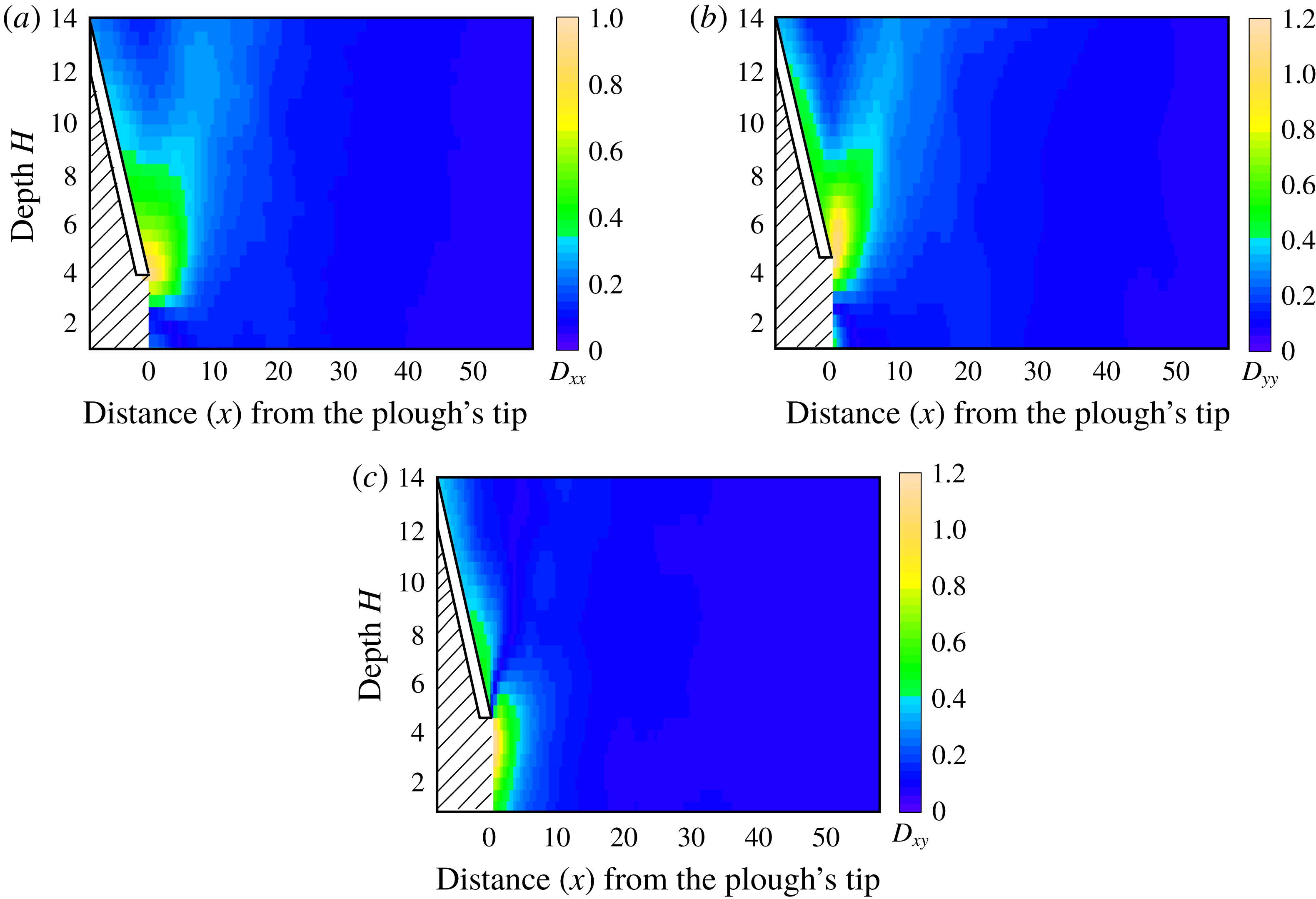
Different components of the strain rate tensor
 $\unicode[STIX]{x1D63F}$
: (a) normal strain rate
 $\unicode[STIX]{x1D60B}_{xx}$
; (b) normal strain rate
 $\unicode[STIX]{x1D60B}_{yy}$
; (c) shear strain rate
 $\unicode[STIX]{x1D60B}_{xy}$
. The plough’s non-dimensional speed
 $v_{c}=10.$
We do not report information in the hatched area.

4.2 Strains
In a continuum description, let
 $\boldsymbol{V}=V_{x}\hat{\boldsymbol{i}}+V_{y}\hat{\boldsymbol{j}}$
be the velocity of a material point at a point
 $\boldsymbol{X}=x\hat{\boldsymbol{i}}+y\hat{\boldsymbol{j}}$
in the reference frame of the plough. The velocity gradient tensor is given by
 $$\begin{eqnarray}\boldsymbol{L}=\frac{\unicode[STIX]{x2202}\boldsymbol{V}}{\unicode[STIX]{x2202}\boldsymbol{X}}.\end{eqnarray}$$
For numerically differentiating the velocity field, as in (4.3), the velocity data are further smoothened by using cubic smoothing splines. The smooth.spline function of the ‘stats’ package in the software R (R Core Team 2013) is employed for this task. The smoothening of the spline fitting is controlled by the parameter spar, with
 $spar=0$
corresponding to an interpolating spline with no smoothening, and
 $spar=1$
implying a linear least squares fit. After some iterations, we found that
 $spar=0.6$
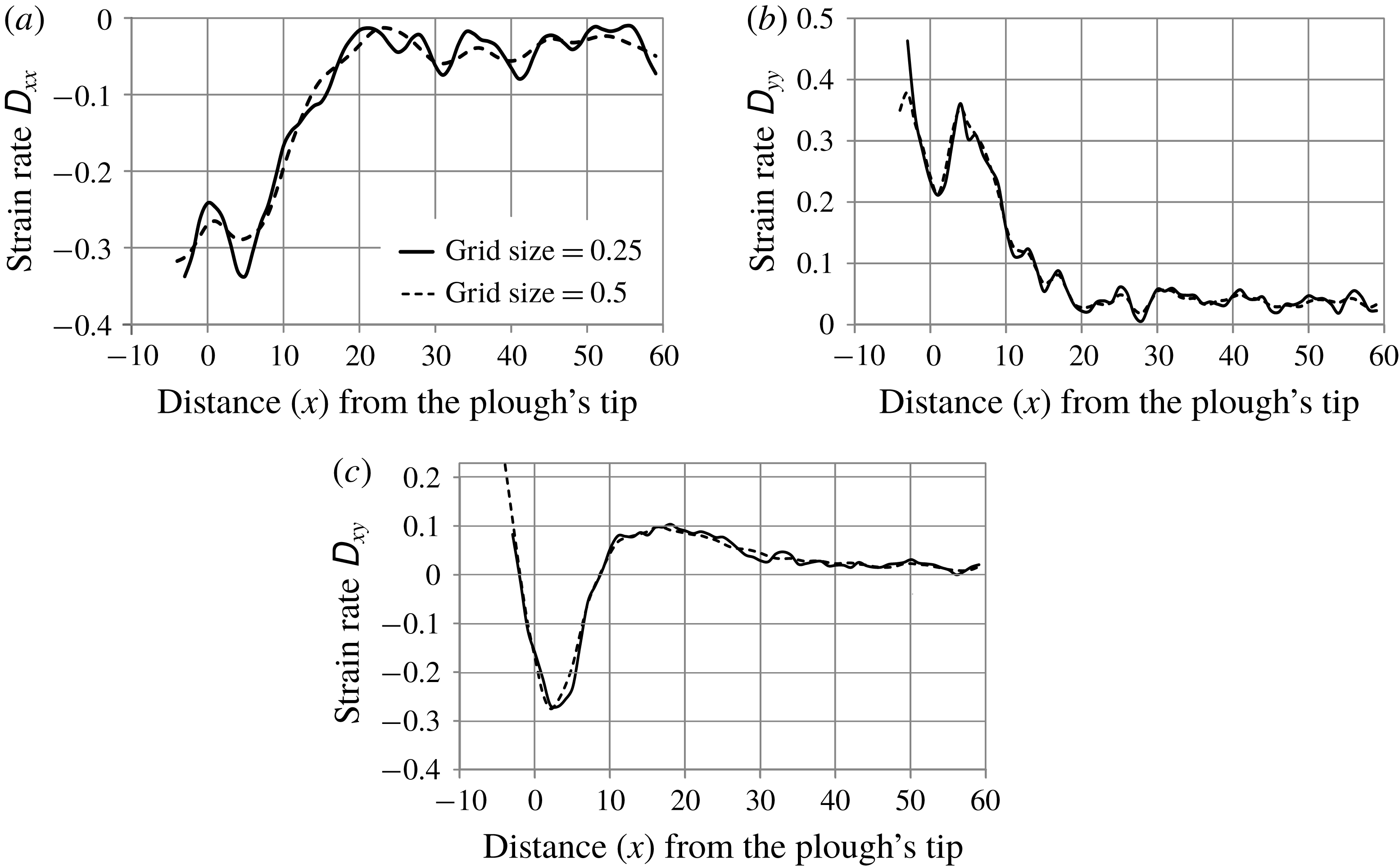
leads to a good fit and gets rid of unwanted fluctuations in the data. Spatial derivatives are then computed numerically. In this context, we note that we have ensured that the grid size that we employ provides an accurate estimate of the strain rates, and this is discussed in appendix A.
The symmetric part of the velocity gradient tensor provides the stretching rate tensor:
 $$\begin{eqnarray}\unicode[STIX]{x1D63F}={\textstyle \frac{1}{2}}(\boldsymbol{L}+\boldsymbol{L}^{\text{T}}).\end{eqnarray}$$
Plots for different components of
 $\unicode[STIX]{x1D63F}$
for one instance of ploughing are shown in figure 6. We observe high strain rates near the tip of the plough. This is also evident from the velocity plots in figure 5, where rapid changes in the velocity field are found near the plough’s tip.
4.3 Variability with grain properties
The ESPM works best when the system is kinematically controlled, so that grain/system parameters (e.g. inter-grain friction, grain size, ploughing speed) do not affect the flow significantly. We will gauge the extent to which these parameters affect the strain rate tensor
 $\unicode[STIX]{x1D63F}$
by calculating the total average relative error
 $$\begin{eqnarray}e_{rel}(f;r_{i})=\left\{\frac{\int _{x=0}^{l}\Vert \overline{f(x)}-f(x,r_{i})\Vert ^{2}\,\text{d}x}{\int _{x=0}^{l}\Vert \overline{f(x)}\Vert ^{2}\,\text{d}x}\right\}^{1/2},\end{eqnarray}$$
where
 $r_{i}$
is
 $i$
th value of a parameter
 $r$
, with
 $i=1\ldots n$
, and
 $f$
is a component of
 $\unicode[STIX]{x1D63F}$
, and
 $$\begin{eqnarray}\overline{f(x)}=\frac{\mathop{\sum }_{i=1}^{n}f(x,r_{i})}{n}\end{eqnarray}$$
is the average of
 $f$
over all
 $r_{i}$
at a given location
 $x$
. We now test to what extent this assumption holds in the context of ploughing.
4.3.1 Grain shape
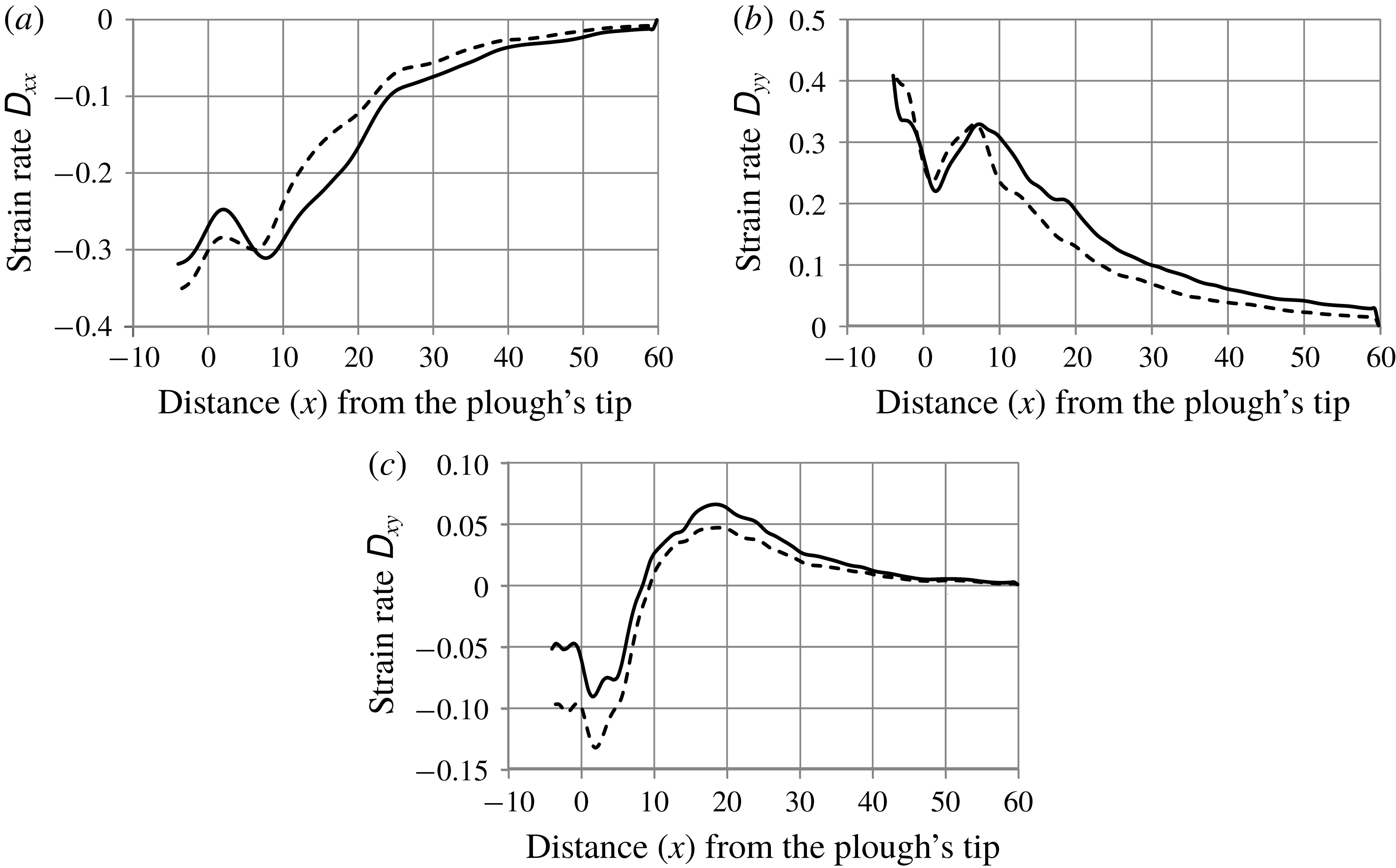
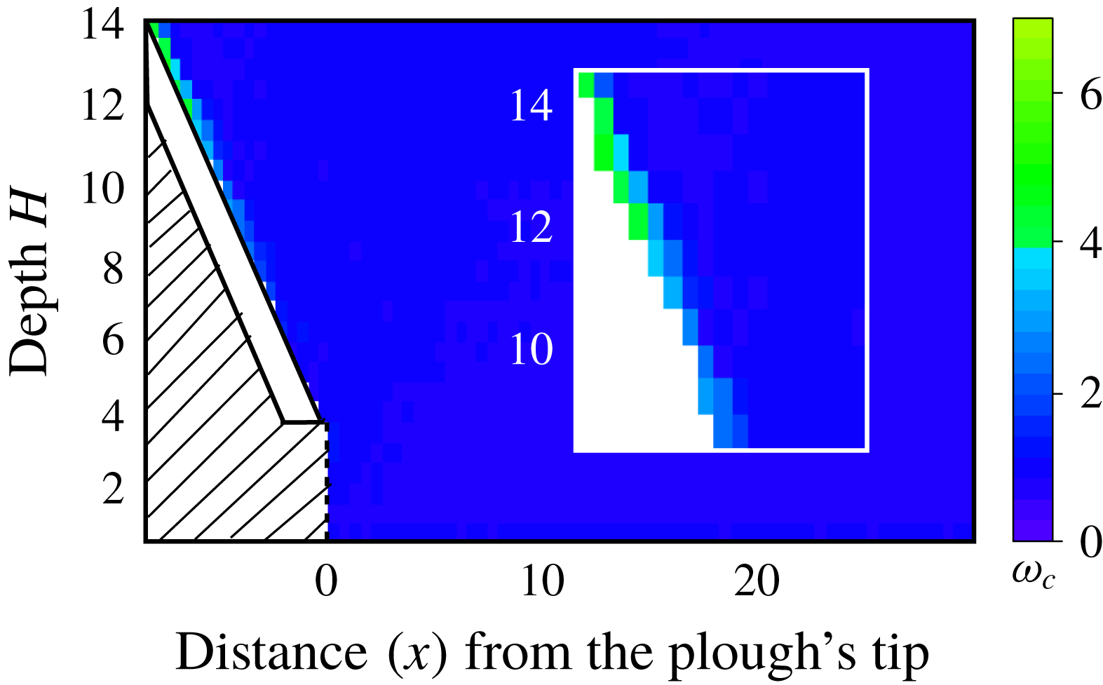
Grain shape is important in DE simulations because circular grains undergo excessive rotation. Various attempts have been made to include shape effects in DE simulations. For example, Pawar (Reference Pawar2013) included rolling resistance between contacting grains, Coetzee & Els (Reference Coetzee and Els2009) utilized compound grains and Obermayr et al. (Reference Obermayr, Dressler, Vrettos and Eberhard2011) employed non-rotating grains. We performed simulations using both rotating and non-rotating grains, and found that restricting grain rotations did not have any significant effect on the strain rates in most of the region of interest; see figure 7. However, as shown in figure 7(c), near the plough’s surface the relative difference in shear strains became somewhat prominent. This is expected, because non-rotating grains undergo significant slipping at the surface of the plough, whereas rotating grains accommodate shear easily by rotating. However, we see from figure 8, that grains undergo rotations only near the plough and, elsewhere, grain rotations are negligible.
Components of the strain rate tensor at points along the line
 $y=9$
when rotating grains (solid lines) and non-rotating grains (dashed lines) are implemented. The plough’s tip is at
 $x=0$
. (a) Normal strain rate
 $\unicode[STIX]{x1D60B}_{xx}$
. (b) Normal strain rate
 $\unicode[STIX]{x1D60B}_{yy}$
. (c) Shear strain rate
 $\unicode[STIX]{x1D60B}_{xy}$
. The plough’s non-dimensional speed
 $v_{c}=10$
, the inter-grain friction
 $\unicode[STIX]{x1D707}=0.5$
and grain diameter
 $d=0.67$
.

The rotation rate
 $\unicode[STIX]{x1D714}_{c}$
of grains. The rotation rate is nearly zero at most places. The plough’s non-dimensional speed
 $v_{c}=10$
. We do not report information in the hatched area. Inset shows the higher strain rates near the plough.

Subsequently, we will perform DE simulations employing non-rotating grains. There are three reasons for this choice. First, we will in § 5 estimate stresses from strain fields through a simple constitutive law which does not include the effects of grain rotation. Thus, a consistent formulation requires that we ignore grain rotation in our simulations. Constitutive laws for granular materials that include grain rotation are complex and, perhaps, unwarranted at present. Second, the excess rotation at the plough’s surface in figure 8 depends on how a flat-faced plough is modelled in DE simulations. We approximate a flat-faced plough by an array of grains that are bonded together and have half the diameter of the larger grains in the bulk; see inset of figure 3. Reducing the diameter of these grains lowers the extent of grain rotation near the plough, thereby bringing DE simulations with non-rotating grains closer to those wherein the grains are free to rotate. Third, Obermayr et al. (Reference Obermayr, Dressler, Vrettos and Eberhard2011) have shown that realistic forces on flat-faced ploughs may be obtained from calibrated DE simulations in which grain rotation is prevented. We too will show in § 6 that proceeding with non-rotating grains gives us a good match with experiments.
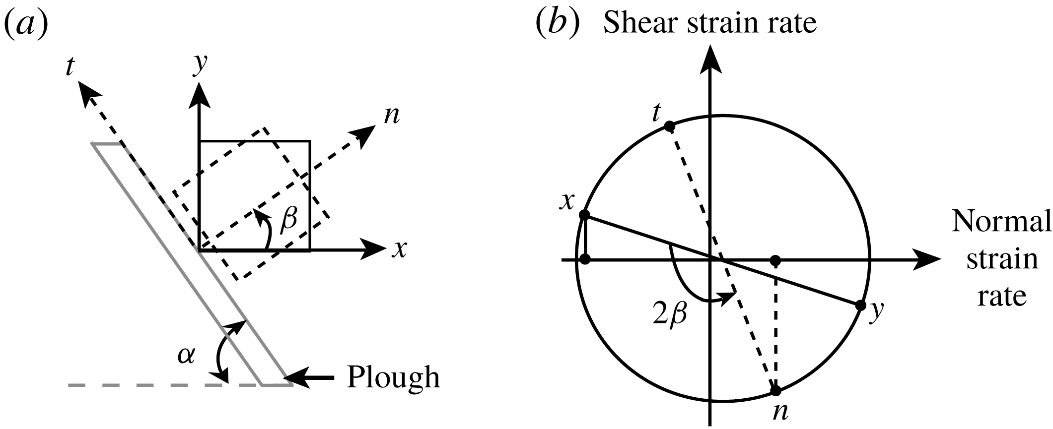
(a) Schematic of continuum elements next to the plough’s surface in
 $x$
–
 $y$
and
 $n$
–
 $t$
coordinate systems. (b) Mohr’s circle transformation to find strain rates in the
 $n$
–
 $t$
system. The angle
 $\unicode[STIX]{x1D6FD}=90^{\circ }-\unicode[STIX]{x1D6FC}$
, where
 $\unicode[STIX]{x1D6FC}=50^{\circ }$
is the tool angle in our simulations, and
 $D_{n}$
and
 $D_{t}$
represent normal and shear strain rates, respectively. In our sign convention, a negative ordinate at the
 $x$
or
 $n$
points indicates a positive shear strain rate (Crandall, Dahl & Dill Reference Crandall, Dahl and Dill1960).

Finally, a general remark. Figure 7 shows that small, negative shear strain rates are seen near the plough. This runs counter to our expectations of a large, positive shear rate when the tool angle
 $\unicode[STIX]{x1D6FC}$
is not shallow. This anomaly is explained by realizing that the
 $x{-}y$
coordinate system, in which the components of the strain rate tensor are evaluated and displayed in figure 7, is not aligned with the normal
 $(n)$
and tangent
 $(t)$
directions of the plough. When the strain rate components are expressed in the
 $n$
–
 $t$
system, we do indeed find a large and positive shear strain rate next to the plough’s surface (see figure 9).
4.3.2 Inter-grain friction
Internal friction is the most important (bulk) constitutive property for a cohesionless granular material. Simulations were carried out for values of inter-grain friction
 $\unicode[STIX]{x1D707}$
ranging from 0.1 to 1. The bulk internal friction angle is expected to grow with increasing
 $\unicode[STIX]{x1D707}$
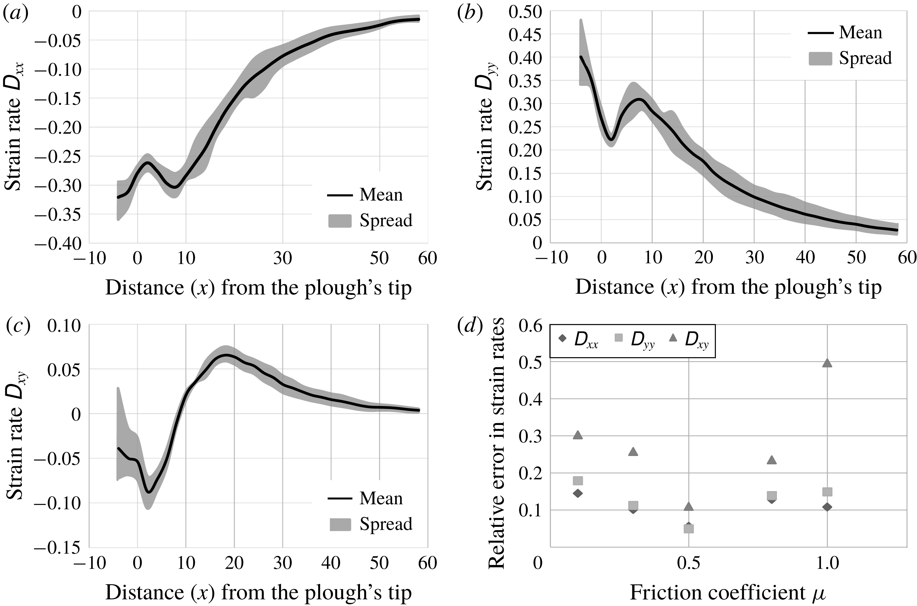
. Figure 10 shows the components of the stretching rate tensor
 $\unicode[STIX]{x1D63F}$
along the horizontal line
 $y=9$
for different values of
 $\unicode[STIX]{x1D707}$
. The variation in normal strain rates is observed to be within 20 % of their mean value, while shear strain rates are within 30 %, except for when
 $\unicode[STIX]{x1D707}=1$
. We proceed by assuming that strain rates may be considered independent of inter-grain friction.
The mean value (black line) and spread about the mean (grey region) of the components of the strain rate tensor
 $\unicode[STIX]{x1D63F}$
at points along the line
 $y=9$
for several values of inter-grain friction
 $\unicode[STIX]{x1D707}$
between 0.1 and 1. The plough’s tip is at
 $x=0$
. (a) Normal strain rate
 $\unicode[STIX]{x1D60B}_{xx}$
. (b) Normal strain rate
 $\unicode[STIX]{x1D60B}_{yy}$
. (c) Shear strain rate
 $\unicode[STIX]{x1D60B}_{xy}$
. (d) Average relative error in components of the strain rate. The plough’s non-dimensional speed
 $v_{c}=10$
.

4.3.3 Grain size
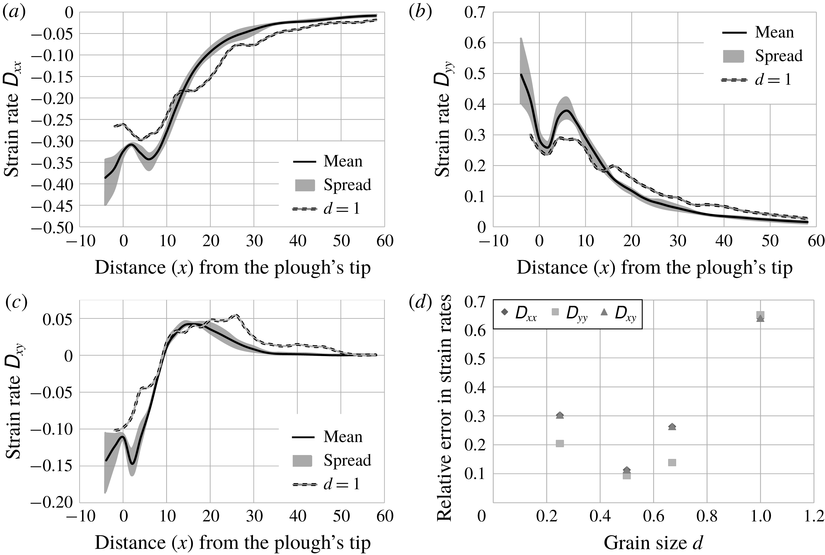
The mean value (black line) and spread about the mean (grey region) of the components of the strain rate tensor
 $\unicode[STIX]{x1D63F}$
at points along the line
 $y=9$
for several grain diameters
 $d$
between 0.25 and 0.67. The strain rates for
 $d=1$
are shown separately. The number of grains correspondingly reduced from 64 000 to 4000. (a) Normal strain rate
 $\unicode[STIX]{x1D60B}_{xx}$
. (b) Normal strain rate
 $\unicode[STIX]{x1D60B}_{yy}$
. (c) Shear strain rate
 $\unicode[STIX]{x1D60B}_{xy}$
. (d) Average relative error in component of strain rate. The plough’s non-dimensional speed
 $v_{c}=10$
.

Simulations were performed for large grain diameters
 $d$
of 1, 0.67, 0.5 and 0.25. The ratio of large to small grain diameter was maintained at 1:0.7. As figure 11 shows, there is a drastic change in strain rates when grain size
 $d$
is decreased from 1 to 0.67. However, further decrease in grain size
 $d$
causes the strain rates to saturate. Therefore,
 $d$
is taken to be 0.67 or less in our simulations.
4.3.4 Polydispersity
Simulations were carried out for various mixing ratios of differently sized grains. Again, different polydispersities did not have any significant effect on strain rates. Monodisperse granular beds, however, produced different results because of regular lattice formation. Thus, polydispersity of 10 % is maintained in our simulations, as it was enough to avoid lattice formation.
4.3.5 Contact stiffness
Strain rates saturate for values of non-dimensional normal contact stiffness
 $k_{n}$
greater than
 $10^{6}$
. Moreover, in the case of frictional particles, Tripathi & Khakhar (Reference Tripathi and Khakhar2010) reported that the effect of contact stiffness on granular flow is small once
 $k_{n}\geqslant 2\times 10^{5}$
. Thus,
 $k_{n}$
is taken to be
 $10^{6}$
in DE simulations. Most naturally occurring grains have values of stiffness much greater than
 $10^{6}$
, so our approach is consistent.
4.3.6 Ploughing speed
Strain rates do change with ploughing speed. This is also in agreement with Percier et al. (Reference Percier, Manneville, McElwaine, Morris and Taberlet2011). Strain rates for different ploughing speeds are plotted in figure 12. At smaller velocities, deformations get time to propagate to larger distances, whereas at larger velocities deformations are unable to reach that far. The non-dimensional velocities in figure 12 vary from 0.1 to 20 which corresponds to the range
 $0.8$
–
 $16~\text{m}~\text{s}^{-1}$
when inter-grain friction
 $\unicode[STIX]{x1D707}=0.5$
and grain diameter
 $d=0.67$
. Therefore, incorporating the correct ploughing speed in the simulations is necessary for accurate prediction of strain rates.
The mean value (black line) and the spread about the mean (grey region) of the components of the strain rate tensor
 $\unicode[STIX]{x1D63F}$
along the line
 $y=9$
for five different ploughing velocities
 $v_{c}$
between 0.1 and 10. (a) Normal strain rate
 $\unicode[STIX]{x1D60B}_{xx}$
. (b) Normal strain rate
 $\unicode[STIX]{x1D60B}_{yy}$
. (c) Shear strain rate
 $\unicode[STIX]{x1D60B}_{xy}$
. (d) Average relative error in component of strain rate. The inter-grain friction
 $\unicode[STIX]{x1D707}=0.5$
and grain diameter
 $d=0.67$
.

5 Continuum model
5.1 Rheology
We now develop a continuum description for the flowing granular material. This will help find stresses in the bulk when combined with strain rates found from DE simulations.
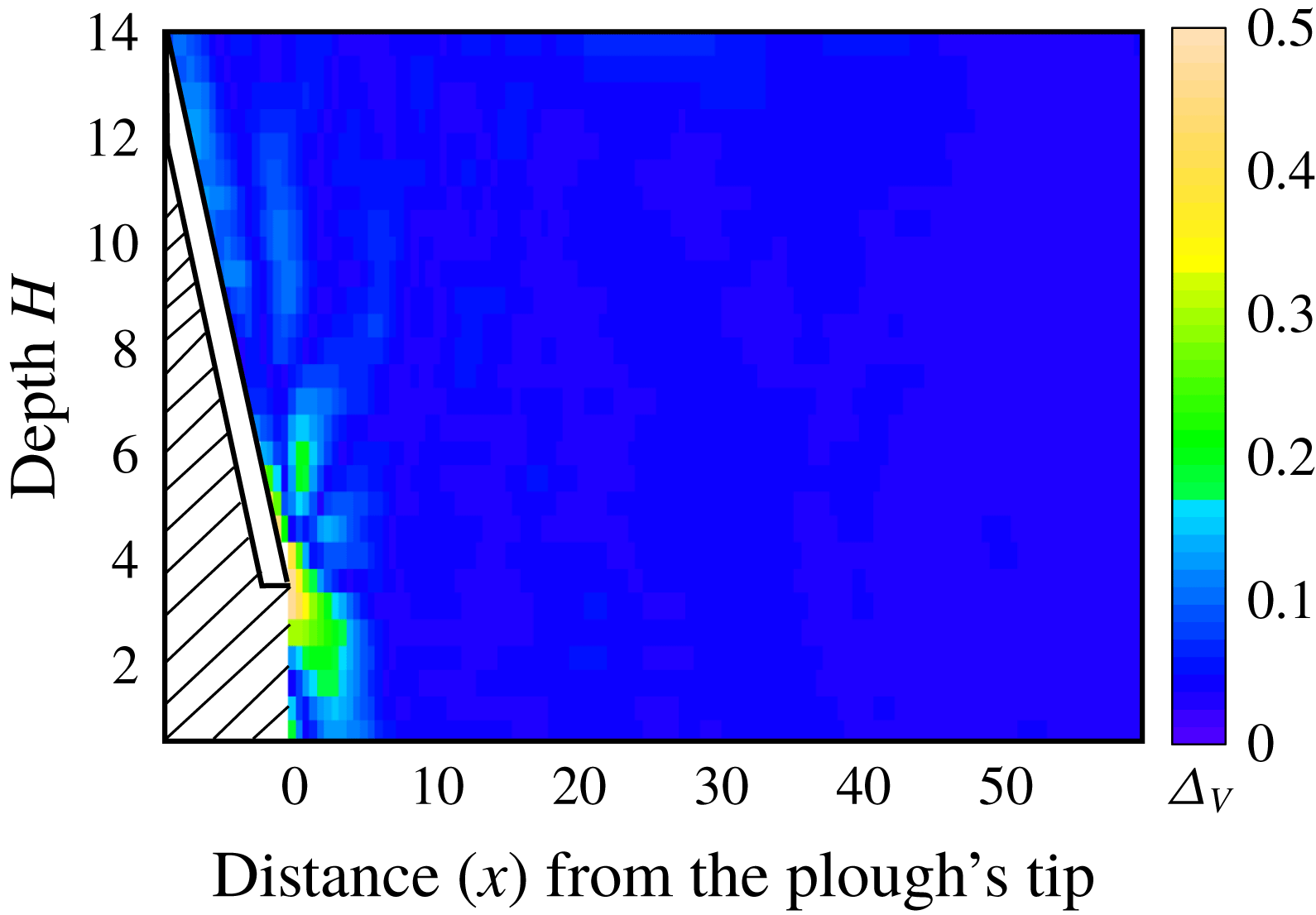
The transition during ploughing from initial solid-like granular bed to a flowing material requires an appropriate constitutive model. We model the granular bed as a pressure-dependent Bingham fluid in which both yield stress and friction during flow depend on the local pressure. The Bingham fluid remains rigid until the stress state violates a yield condition and begins to flow post-yield. We assume for simplicity that the flow post-yield preserves volume. To verify this assumption, we find the dilatation as the trace of the strain rate field estimated from our DE simulations. The result is shown in figure 13 and we observe that, to a great extent, the volume in the bulk does remain preserved. The maximum dilatation is found at the tip of the plough. However, we do not expect accurate estimation of dilatation to have a significant bearing upon the forces exerted on the plough, and this expectation has been endorsed by Coetzee (Reference Coetzee2014) through detailed discrete and continuum simulations.
Time-averaged dilatation
 $\unicode[STIX]{x0394}_{V}$
. The plough’s non-dimensional speed
 $v_{c}=10$
. We do not report information in the hatched area.

Sharma (Reference Sharma2017, § 2.10.1) shows that the post-yield stress in the granular bed when modelled as above is
 $$\begin{eqnarray}\unicode[STIX]{x1D748}=-p\mathbf{1}+kp\frac{\unicode[STIX]{x1D63F}}{|\unicode[STIX]{x1D63F}|},\end{eqnarray}$$
where the pressure
 $$\begin{eqnarray}p=-{\textstyle \frac{1}{3}}\text{tr}\,\unicode[STIX]{x1D748},\end{eqnarray}$$
the parameter
 $$\begin{eqnarray}k=\frac{2\sqrt{6}\sin \unicode[STIX]{x1D711}}{3-\sin \unicode[STIX]{x1D711}}\end{eqnarray}$$
in terms of the soil’s internal friction angle
 $\unicode[STIX]{x1D711}$
and, in indical notation,
 $|\unicode[STIX]{x1D63F}|^{2}=\unicode[STIX]{x1D60B}_{ij}\unicode[STIX]{x1D60B}_{ij}$
. Thus, knowing the strain rate
 $\unicode[STIX]{x1D63F}$
and pressure
 $p$
will allow us to compute the stress
 $\unicode[STIX]{x1D748}$
. We estimate the pressure
 $p$
in the next section.
The constitutive law (5.1) has been employed to model flowing grains in the past (e.g. Schaeffer Reference Schaeffer1987; Sharma Reference Sharma2017). The law (5.1) is very similar to the rheology proposed by Jop et al. (Reference Jop, Forterre and Pouliquen2006) with the key difference being that here
 $k$
replaces the friction coefficient
 $\unicode[STIX]{x1D707}(I)$
of Jop et al. (Reference Jop, Forterre and Pouliquen2006), which is a function of the inertial number
 $I$
. The parameter
 $k$
depends on the granular material only through its macroscopic friction angle
 $\unicode[STIX]{x1D711}$
that, in turn, is related to the properties of the constituent grain, but not on the flow rate. The friction coefficient
 $\unicode[STIX]{x1D707}$
, on the other hand, is also affected by the flow rate through the inertial number.
We make the following regarding our choice of the constitutive law. Recent research (Barker et al.
Reference Barker, Schaeffer, Bohorquez and Gray2015) has shown that the
 $\unicode[STIX]{x1D707}(I)$
-rheology is well-posed for intermediate values of
 $I$
, but not for all
 $I$
. The same could be true for the material model (5.1). To this end, we note the following:
(i) Because we do not integrate in time, the ill-posedness will not affect ESPM. Mathematically ill-posed problems suffer from unbounded growth of short-wavelength perturbations, which necessarily leads to grid-dependent numerical results that do not converge as the spatial resolution is enhanced. Thus, the ill-posedness of the constitutive law becomes crucial when numerically integrating the temporal dynamics of a system. Schaeffer and co-workers (Pitman & Schaeffer Reference Pitman and Schaeffer1987; Schaeffer Reference Schaeffer1987; Schaeffer & Pitman Reference Schaeffer and Pitman1988; Thomas & Schaeffer Reference Thomas and Schaeffer1988; Schaeffer Reference Schaeffer1990; Metcalfe et al. Reference Metcalfe, Tennakoon, Kondic, Schaeffer and Behringer2002) studied the time evolution of two- and three-dimensional, incompressible granular and plastic flows. They stated the conditions under which the governing equations become unstable and ill-posed. They considered the Tresca and von Mises yield criterion; it is unknown whether the Drucker–Prager yield criterion that we employ displays the same behaviour. However, in ESPM, the dynamics of the granular material is evolved temporally through DE simulations, not by the numerical integration of the governing continuum equations. The DE simulations provide the velocity data of the grains at any given instant of time. At that given, fixed instant, the velocity data are spatially smoothened to obtain the continuum velocity and strain fields in the granular material. From these continuum fields the stresses everywhere in the granular material, at that given time, are found by invoking an appropriate constitutive law. Thus, the equations governing the dynamics of the granular material in a continuum description are never numerically integrated. As a result, the possible ill-posedness of the constitutive law (5.1) does not, in any way, affect the final results.
(ii) More importantly, ESPM is agnostic to the choice of the constitutive law, and we are free to utilize more specific and/or sophisticated ones, as per our requirements. We prefer to go with the law (5.1) because it is simple, popular, gives reasonable results and serves the purpose of demonstrating ESPM without getting the discussion mired in the complexity of detailed rheological modelling of granular flows.
In closing, it is important to emphasize that the material model is not tuned to a specific application, which would not be the case if we were to calibrate the grain parameters in our DE simulations.
5.2 Pressure
The linear momentum balances in the x and y directions are, respectively,
 $$\begin{eqnarray}\frac{\unicode[STIX]{x2202}\unicode[STIX]{x1D70E}_{xx}}{\unicode[STIX]{x2202}x}+\frac{\unicode[STIX]{x2202}\unicode[STIX]{x1D70E}_{xy}}{\unicode[STIX]{x2202}y}=\unicode[STIX]{x1D70C}a_{x}\end{eqnarray}$$
and
 $$\begin{eqnarray}\frac{\unicode[STIX]{x2202}\unicode[STIX]{x1D70E}_{xy}}{\unicode[STIX]{x2202}x}+\frac{\unicode[STIX]{x2202}\unicode[STIX]{x1D70E}_{yy}}{\unicode[STIX]{x2202}y}=\unicode[STIX]{x1D70C}(a_{y}+g),\end{eqnarray}$$
where
 $a_{x}$
and
 $a_{y}$
are the x and y components of the acceleration field
 $\boldsymbol{a}$
obtained from (4.2),
 $g$
is the acceleration due to gravity and
 $\unicode[STIX]{x1D70C}$
is the bulk density. Substituting (5.1) into the the above and eliminating
 $\unicode[STIX]{x2202}p/\unicode[STIX]{x2202}y$
, we obtain
 $$\begin{eqnarray}\displaystyle & & \displaystyle \frac{\unicode[STIX]{x2202}p}{\unicode[STIX]{x2202}x}\left\{\left(k\frac{\unicode[STIX]{x1D60B}_{xx}}{|\unicode[STIX]{x1D63F}|}-1\right)\left(1-k\frac{\unicode[STIX]{x1D60B}_{yy}}{|\unicode[STIX]{x1D63F}|}\right)+k^{2}\left(\frac{\unicode[STIX]{x1D60B}_{xy}}{|\unicode[STIX]{x1D63F}|}\right)^{2}\right\}+k^{2}p\left\{\frac{\unicode[STIX]{x2202}}{\unicode[STIX]{x2202}y}\left(\frac{\unicode[STIX]{x1D60B}_{yy}}{|\unicode[STIX]{x1D63F}|}\right)+\frac{\unicode[STIX]{x2202}}{\unicode[STIX]{x2202}x}\left(\frac{\unicode[STIX]{x1D60B}_{xy}}{|\unicode[STIX]{x1D63F}|}\right)\right\}\frac{\unicode[STIX]{x1D60B}_{xy}}{|\unicode[STIX]{x1D63F}|}\nonumber\\ \displaystyle & & \displaystyle \qquad +\,kp\left\{\frac{\unicode[STIX]{x2202}}{\unicode[STIX]{x2202}x}\left(\frac{\unicode[STIX]{x1D60B}_{xx}}{|\unicode[STIX]{x1D63F}|}\right)+\frac{\unicode[STIX]{x2202}}{\unicode[STIX]{x2202}y}\left(\frac{\unicode[STIX]{x1D60B}_{xy}}{|\unicode[STIX]{x1D63F}|}\right)\right\}\left(1-k\frac{\unicode[STIX]{x1D60B}_{yy}}{|\unicode[STIX]{x1D63F}|}\right)\nonumber\\ \displaystyle & & \displaystyle \quad =\unicode[STIX]{x1D70C}a_{x}\left(1-k\frac{\unicode[STIX]{x1D60B}_{yy}}{|\unicode[STIX]{x1D63F}|}\right)+k\unicode[STIX]{x1D70C}\frac{\unicode[STIX]{x1D60B}_{xy}}{|\unicode[STIX]{x1D63F}|}(a_{y}+g).\end{eqnarray}$$
The strain rates, acceleration and density are known from the continuum kinematic fields obtained from DE simulations and the rheology assumed in § 5.1. Thus, the above equation may now be integrated to find the pressure
 $p$
. This we discuss next.
5.2.1 Integration scheme
The pressure
 $p$
at a fixed depth
 $y$
may be found by integrating (5.6) with respect to
 $x$
over the region that has yielded and is flowing. In a Bingham fluid, we need to distinguish between unyielded and flowing regions. The post-yield rheology (5.1) and the differential equation (5.6) for the pressure
 $p$
are applicable only in the flowing region.
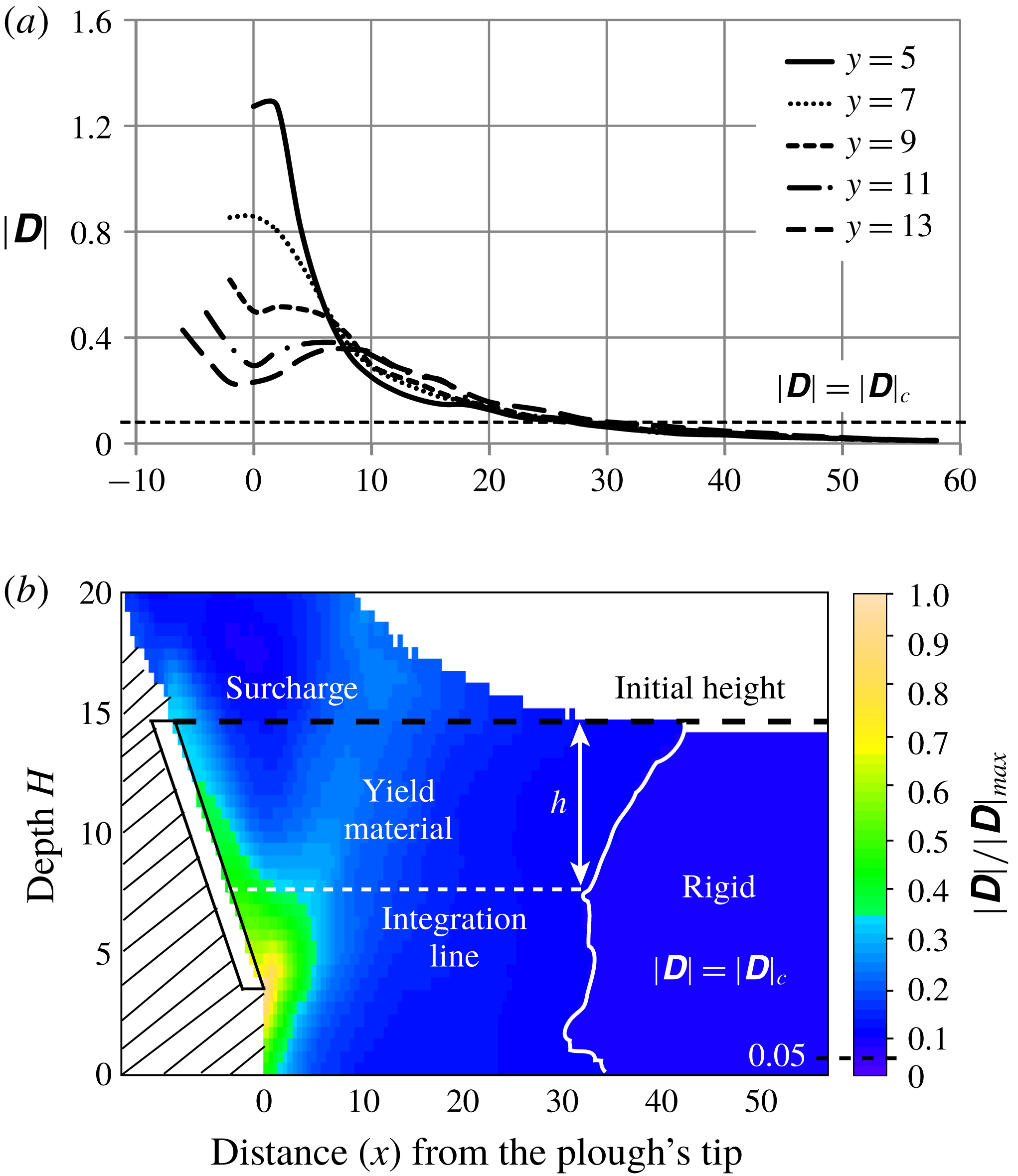
Distinguishing between yielded and unyielded regions. (a) The magnitude of the strain rate tensor
 $|\unicode[STIX]{x1D63F}|$
with distance from tool tip at different depths
 $y$
. The line
 $|\unicode[STIX]{x1D63F}|=|\unicode[STIX]{x1D63F}|_{c}$
, with
 $|\unicode[STIX]{x1D63F}|_{c}=0.05|\unicode[STIX]{x1D63F}|_{max}$
is also shown. Here, we find that
 $|\unicode[STIX]{x1D63F}|_{max}=1.7$
at
 $y=4$
(not shown). (b) The magnitude of strain rate
 $|\unicode[STIX]{x1D63F}|$
in the entire material. The yielded boundary obtained by setting
 $|\unicode[STIX]{x1D63F}|_{c}=0.05|\unicode[STIX]{x1D63F}|_{max}$
is also shown. The granular material which accumulates above the initial height of the granular bed is defined as the surcharge. The plough’s non-dimensional speed
 $v_{c}=10.$
We do not report information in the hatched area.

We thus need to find the extent of the flowing region. Distinction between unyielded and flowing regions may be made on the basis of strain rates, e.g. through
 $|\unicode[STIX]{x1D63F}|$
, which is a measure of the extent of flow. In the unyielded region
 $|\unicode[STIX]{x1D63F}|$
should, theoretically, be zero. In figure 14(a),
 $|\unicode[STIX]{x1D63F}|$
is plotted as a function of the distance from the plough for different depths. We see that
 $|\unicode[STIX]{x1D63F}|$
far away from the plough stays nearly zero, but increases sharply as we move towards the plough. In granular materials forces travel through force chains (Liu et al.
Reference Liu, Nagel, Schecter, Coppersmith, Majumdar, Narayan and Witten1995), so that small fluctuations are always present, which causes small non-zero values of
 $|\unicode[STIX]{x1D63F}|$
to be found even in far away regions where the granular material, for all practical purposes, has still not yielded. We therefore define a critical value
 $|\unicode[STIX]{x1D63F}|_{c}$
and material with
 $|\unicode[STIX]{x1D63F}|>|\unicode[STIX]{x1D63F}|_{c}$
is said to be flowing, else it has not yielded. We set
 $|\unicode[STIX]{x1D63F}|_{c}=\unicode[STIX]{x1D6FD}|\unicode[STIX]{x1D63F}|_{max}$
, where
 $|\unicode[STIX]{x1D63F}|_{max}$
is the maximum observed value of
 $|\unicode[STIX]{x1D63F}|$
at a given ploughing speed. A plot with
 $\unicode[STIX]{x1D6FD}=0.05$
showing the variation of
 $|\unicode[STIX]{x1D63F}|$
is shown in figure 14(b). The region to the left of the boundary
 $|\unicode[STIX]{x1D63F}|=|\unicode[STIX]{x1D63F}|_{c}$
is flowing while the right-hand side region is, as yet, unyielded.
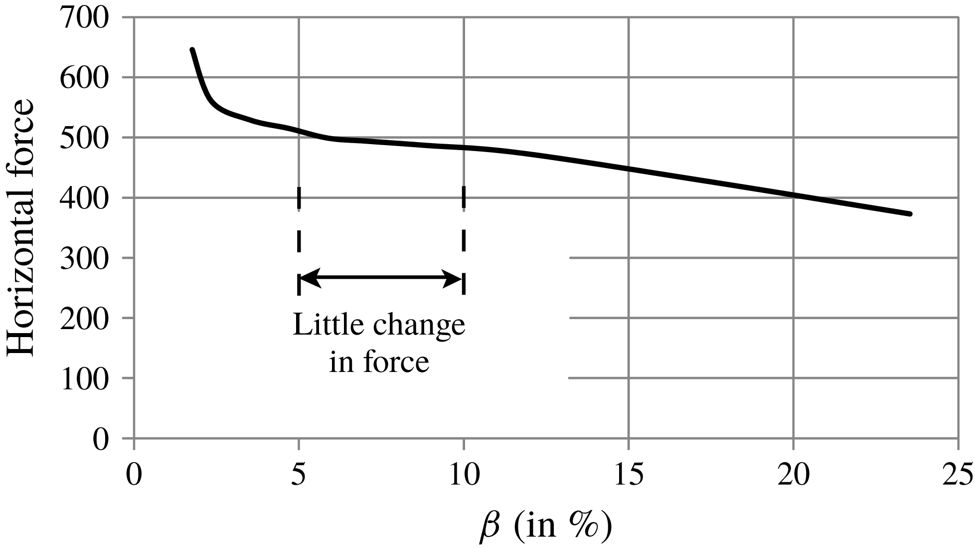
The effect of the choice of
 $|\unicode[STIX]{x1D63F}|_{c}$
on horizontal force calculations (discussed below) is shown in figure 15. We see that the horizontal force is relatively insensitive to the choice of
 $\unicode[STIX]{x1D6FD}$
between 5 % and 10 %. For
 $\unicode[STIX]{x1D6FD}<5\,\%$
, the unyielded region expands and begins affecting the force calculation, as observed by the sudden increase in the horizontal force in figure 15. With
 $\unicode[STIX]{x1D6FD}$
more than 10 %, the force starts decreasing rapidly, which indicates that we are allowing the region identified as unyielded to encroach into a region where material is, in fact, flowing. Thus, we set
 $\unicode[STIX]{x1D6FD}=0.05$
.
Effect of choice of
 $|\unicode[STIX]{x1D63F}|_{c}$
on horizontal force on a plough moving with non-dimensional speed
 $v_{c}=5$
.

To find the pressure
 $p$
we integrate (5.6) numerically from the yield boundary towards the plough along horizontal lines, e.g. the dashed line in figure 14(b), employing the grid constructed in figure 5. Pressure at a point on this boundary is taken to be due to the weight of the granular material above it, i.e. lithostatic. Thus, pressure on the yield boundary is
 $\unicode[STIX]{x1D70C}gh$
, where
 $\unicode[STIX]{x1D70C}$
is the bulk density of the granular bed and
 $h$
is the depth of the point from the free surface (see figure 14
b). The height
 $h$
may be obtained from DE simulations (after appropriate rescaling) or from experiments. In (5.6), we know
 $a_{x}$
,
 $a_{y}$
and
 $\unicode[STIX]{x1D63F}$
at the grid points. The terms involving derivatives of
 $\unicode[STIX]{x1D63F}$
in (5.6) are calculated using finite differences. Step size for integration is therefore the same as the grid size in figure 5. Integrating (5.6) allows us to estimate the pressure everywhere in the flowing region. We note that the pressure in the rigid and surcharge regions is also taken to be lithostatic.
5.2.2 Comparison
Qualitative validation of the pressure field obtained in the previous section may be obtained by comparing with pressure found directly from our uncalibrated DE simulations. For a quantitative match, it is necessary to tune the grain properties employed in our DE simulations to the bulk internal friction angle employed in our continuum model, which has not been done. In the literature, available calibrated grain data are for three-dimensional ploughing (e.g. Obermayr et al. Reference Obermayr, Dressler, Vrettos and Eberhard2011), while ours is a two-dimensional system.
The average pressure on grain
 $i$
may be found from a DE simulation by (e.g. Bhateja et al.
Reference Bhateja, Sharma and Singh2016)
 $$\begin{eqnarray}p_{i}=\frac{1}{S_{i}}\mathop{\sum }_{j}f_{ij}^{n},\end{eqnarray}$$
where
 $f_{ij}^{n}$
is the normal force exerted upon grain
 $i$
by grain
 $j$
that abuts grain
 $i$
and
 $S_{i}$
is the surface area of the
 $i$
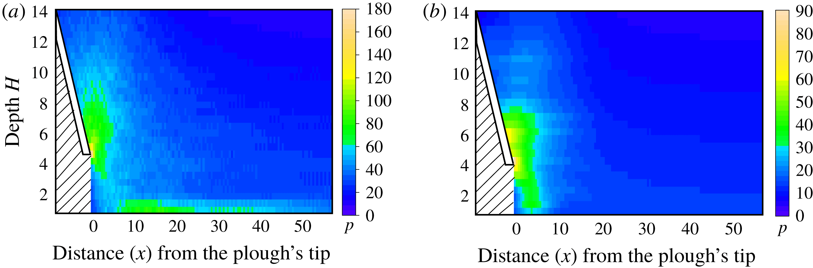
th grain. This average pressure is calculated for every grain at every time step and then averaged over space and time to, finally, provide the pressure field. Figure 16(a) shows the pressure variation obtained directly from our uncalibrated DE simulation. We find a good qualitative match with the continuum pressure field in figure 16(b) that is obtained by solving (5.6). Both figures predict that a high-pressure region develops near the tip of the plough.
In passing, we note that in figure 16(a) a high-pressure region is seen at the bottom of the granular bed in DE simulations, but not in the continuum pressure field estimated by ESPM. We believe that this is because the flow field is not well resolved near the channel’s base.
Comparison of pressure
 $p$
in the bulk obtained (a) from DE simulations with
 $\unicode[STIX]{x1D707}=0.3$
and (b) by following the procedure of § 5.2 with
 $\unicode[STIX]{x1D711}=25^{\circ }$
. In each case the plough’s non-dimensional speed
 $v_{c}=10$
. We do not report information in the hatched area.

5.3 Forces
Once pressure is known everywhere, equation (5.1) allows us to find normal and shear stress everywhere in the plastic region. The normal force
 $F_{N}$
on the tool’s surface (see figure 1) may then be estimated by integrating the normal stress component
 $\unicode[STIX]{x1D70E}_{nn}$
over its surface:
 $$\begin{eqnarray}F_{N}=\int _{S_{t}}\unicode[STIX]{x1D70E}_{nn}\,\text{d}A,\end{eqnarray}$$
where
 $S_{t}$
is the surface area of the plough in contact with the granular material. The normal stress component is related to stress components in the
 $x$
–
 $y$
coordinate system (see figure 1) by
 $$\begin{eqnarray}\unicode[STIX]{x1D70E}_{nn}={\textstyle \frac{1}{2}}(\unicode[STIX]{x1D70E}_{xx}+\unicode[STIX]{x1D70E}_{yy})-{\textstyle \frac{1}{2}}(\unicode[STIX]{x1D70E}_{xx}-\unicode[STIX]{x1D70E}_{yy})\cos 2\unicode[STIX]{x1D6FC}+\unicode[STIX]{x1D70E}_{xy}\sin 2\unicode[STIX]{x1D6FC},\end{eqnarray}$$
which follows from the Mohr circle, and where
 $\unicode[STIX]{x1D6FC}$
is the inclination of the plough. Similarly, from the Mohr circle, the shear stress component
 $$\begin{eqnarray}\unicode[STIX]{x1D70E}_{nt}=-{\textstyle \frac{1}{2}}(\unicode[STIX]{x1D70E}_{xx}-\unicode[STIX]{x1D70E}_{yy})\sin 2\unicode[STIX]{x1D6FC}+\unicode[STIX]{x1D70E}_{xy}\cos 2\unicode[STIX]{x1D6FC},\end{eqnarray}$$
which provides the total shear force on the tool as
 $$\begin{eqnarray}F_{T}=\int _{S_{t}}\unicode[STIX]{x1D70E}_{nt}\text{d}A.\end{eqnarray}$$
Knowledge of
 $F_{N}$
and
 $F_{T}$
allows us to compute horizontal and vertical forces on the plough in a straightforward manner.
6 Results and discussion
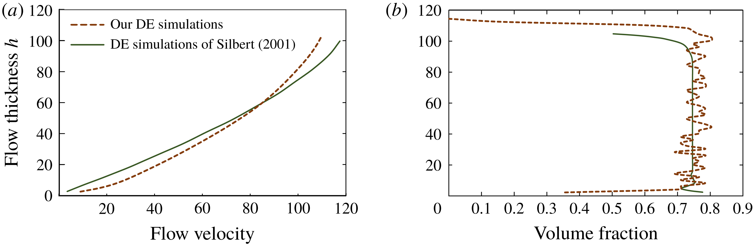
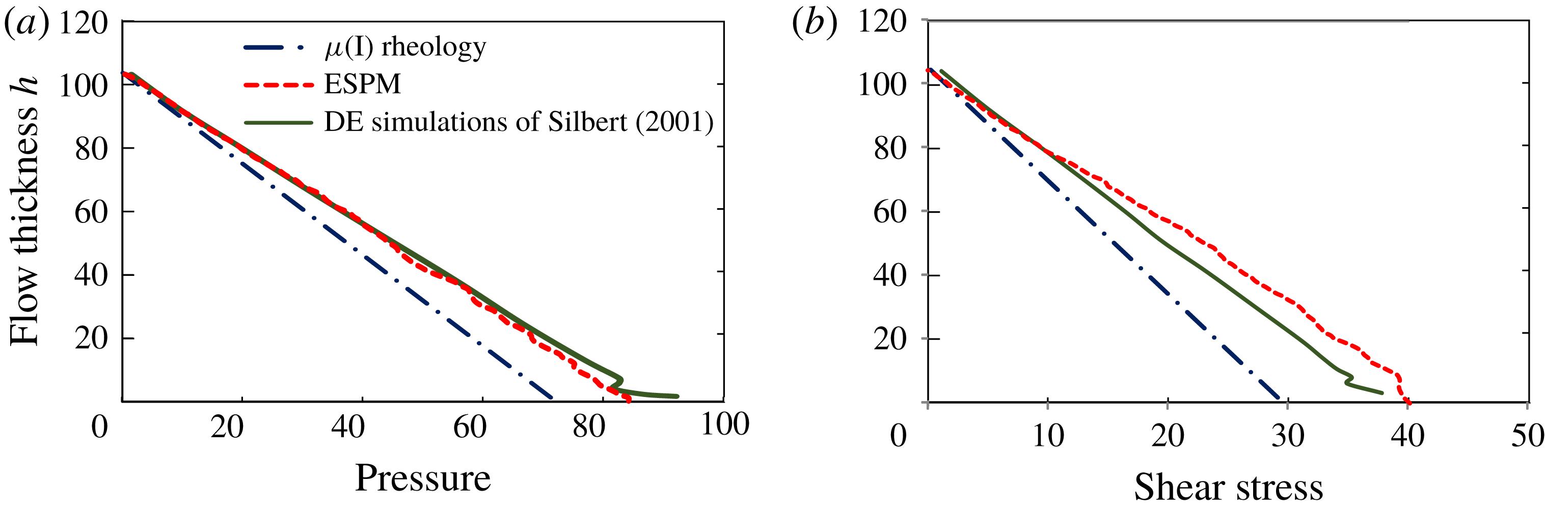
As a preliminary exercise to build confidence in ESPM in the context of a well-studied granular system, we have utilized ESPM to investigate granular flow down an inclined plane. We find an excellent match with theoretical predictions predicated upon the
 $\unicode[STIX]{x1D707}(I)$
-rheology (Jop et al.
Reference Jop, Forterre and Pouliquen2006; Pouliquen & Forterre Reference Pouliquen and Forterre2009), and this is discussed in detail in appendix B. Here we proceed to compare the ploughing forces predicted by ESPM against those measured in experiments and estimated by calibrated DE simulations.
6.1 Calibrated DE simulations
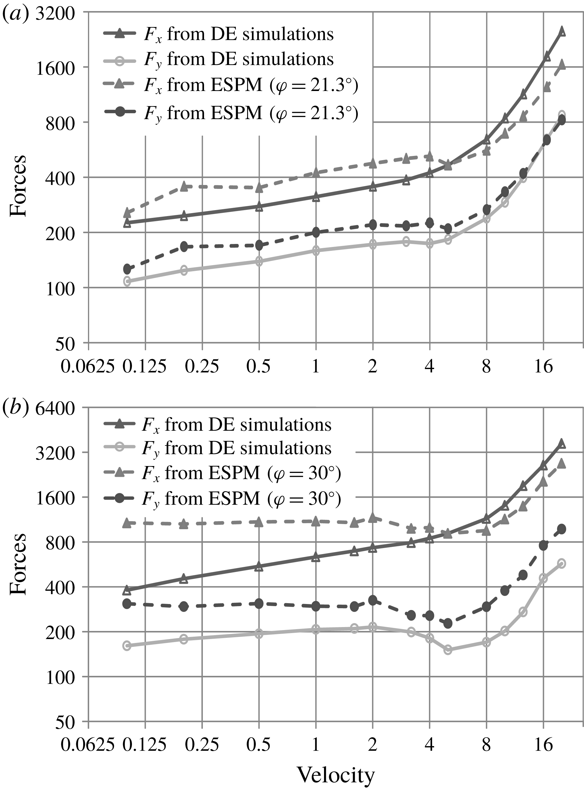
Comparison of ploughing forces computed from ESPM and DE simulations. Here,
 $F_{x}$
and
 $F_{y}$
represent the horizontal and the vertical forces on the plough, respectively. (a) Steel balls. ESPM:
 $\unicode[STIX]{x1D711}=21.3^{\circ }$
; DE simulations:
 $\unicode[STIX]{x1D707}=0.07$
. (b) Gravel. ESPM:
 $\unicode[STIX]{x1D711}=30^{\circ }$
; DE simulations:
 $\unicode[STIX]{x1D707}=0.3$
.

Obermayr et al. (Reference Obermayr, Dressler, Vrettos and Eberhard2011) carried out three-dimensional simulations and experiments with steel balls and gravel, in which a vertical plate cuts through a granular bed. The internal friction angles measured experimentally from triaxial compression tests were
 $\unicode[STIX]{x1D711}=21.3^{\circ }$
for steel balls and
 $\unicode[STIX]{x1D711}=30^{\circ }$
for gravel. The parameters of their DE simulations were calibrated by matching them with triaxial tests. Consequently, the microscopic inter-grain friction to be utilized in DE simulations was determined to be
 $\unicode[STIX]{x1D707}=0.07$
for steel balls and
 $\unicode[STIX]{x1D707}=0.3$
for gravel. Obermayr et al. restricted grain rotations in their DE simulations.
In this section, we will compare the predictions for ploughing forces obtained from ESPM with those of calibrated DE simulations. To this end, we take the calibrated data from Obermayr et al. (Reference Obermayr, Dressler, Vrettos and Eberhard2011) and perform two separate sets of DE simulations of two-dimensional ploughing: one with
 $\unicode[STIX]{x1D707}=0.07$
to model steel balls and the other with
 $\unicode[STIX]{x1D707}=0.3$
for gravel. Corresponding to these two DE simulations, we set the bulk internal friction angles in our ESPM calculations as, respectively,
 $\unicode[STIX]{x1D711}=21.3^{\circ }$
and
 $\unicode[STIX]{x1D711}=30^{\circ }$
. Simulations are now performed for a plough with angle
 $\unicode[STIX]{x1D6FC}=50^{\circ }$
over a range of ploughing speeds utilizing the preceding two values of
 $\unicode[STIX]{x1D711}$
; this is supposed to imitate ploughing of steel and gravel, respectively. Because we are employing calibrated data, it may be expected that forces computed by our DE simulations should match ESPM predictions. However, we note a major difference between our DE simulations and those of Obermayr et al.: the latter were three-dimensional simulations with spherical grains, while we restrict ourselves to two dimensions with disc-shaped grains. Thus, the calibrated microscopic inter-grain friction obtained by Obermayr et al. may not be applicable to our two-dimensional system.
In figure 17, horizontal and vertical forces computed directly from our DE simulations (with calibrated data from Obermayr et al.) are compared with forces obtained from ESPM. The ESPM curves show good qualitative match with simulations, but some quantitative deviations are observed, e.g. gravel in figure 17(b). We believe that the quantitative mismatch is due to our using calibrated data from Obermayr et al. (Reference Obermayr, Dressler, Vrettos and Eberhard2011), obtained originally for three-dimensional simulations, in our two-dimensional DE simulations. Furthermore, we assumed a simple rheological model in our ESPM calculations. We expect that employing grain data correctly calibrated for a two-dimensional system, along with a more detailed rheology will provide a closer match.
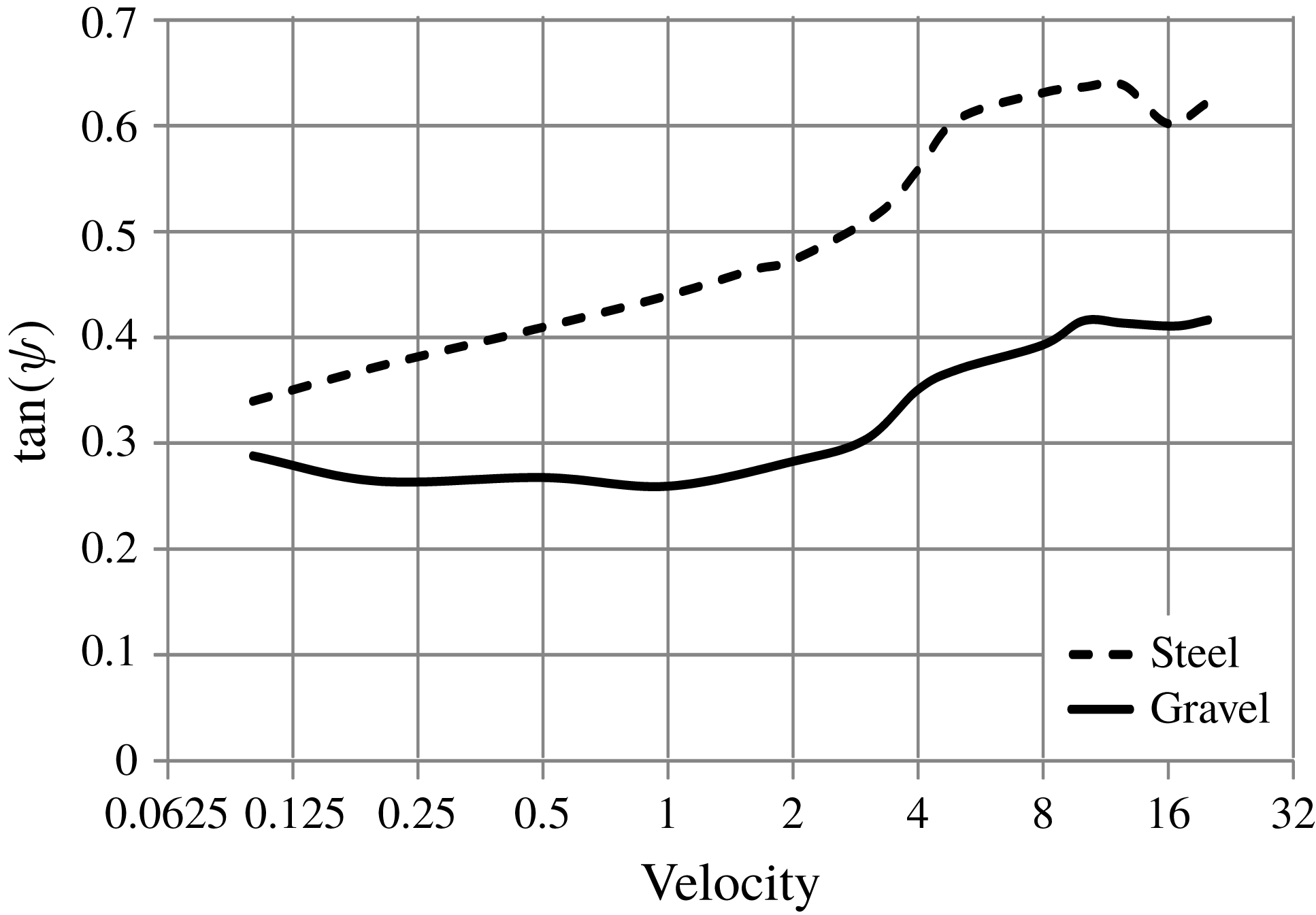
Variation of
 $\unicode[STIX]{x1D713}$
defined in (6.1) with ploughing velocity for simulations with steel (
 $\unicode[STIX]{x1D707}=0.07$
) and gravel (
 $\unicode[STIX]{x1D707}=0.3$
).

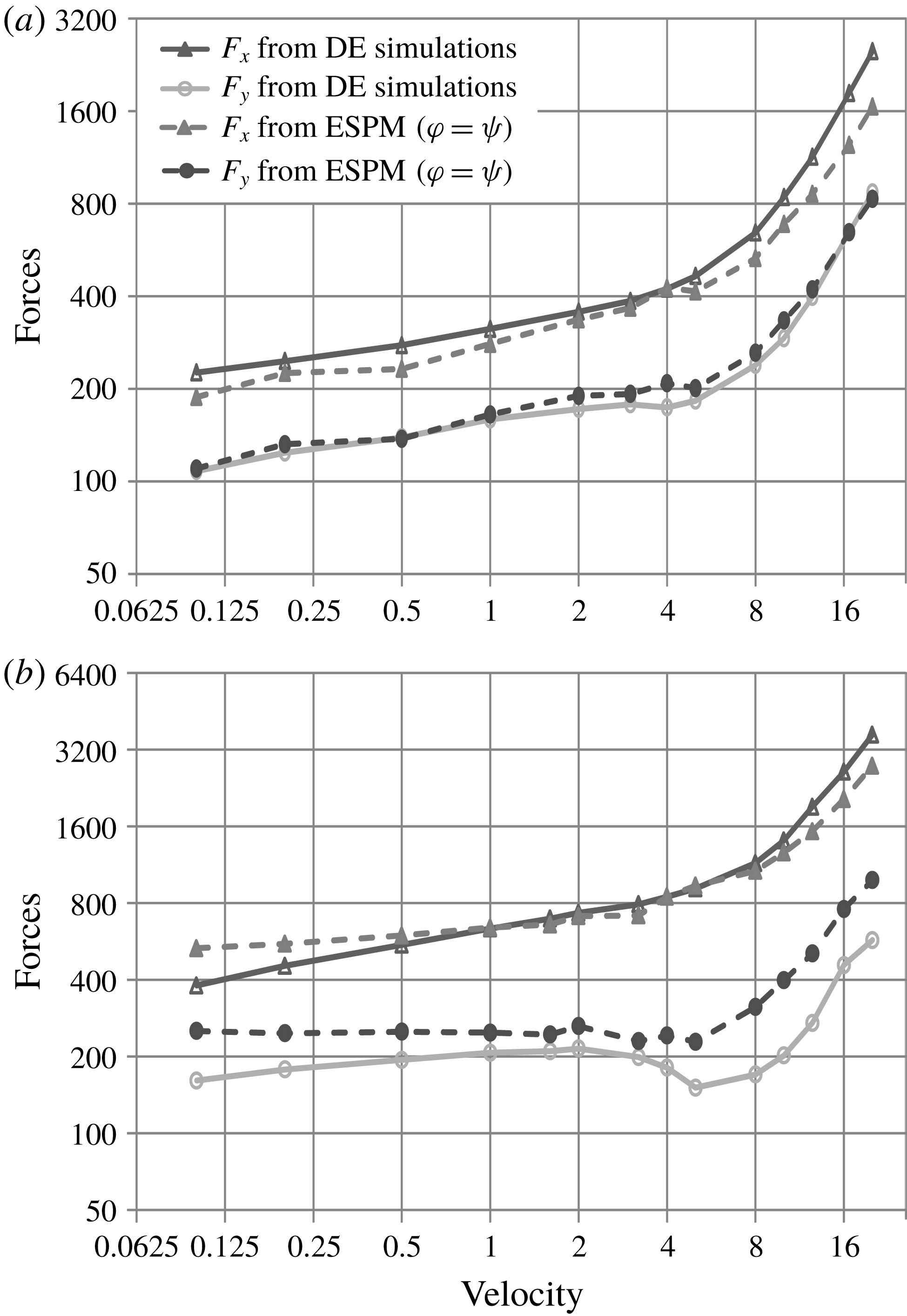
We now report an interesting observation. Predictions from ESPM are greatly improved if, instead of using the experimentally measured internal friction angle in ESPM computations, we set the friction angle
 $\unicode[STIX]{x1D711}=\unicode[STIX]{x1D713}$
in (5.3), where
 $$\begin{eqnarray}\tan \unicode[STIX]{x1D713}=\frac{F_{N}}{F_{T}}\end{eqnarray}$$
is the plough-grain friction angle found from the normal (
 $F_{N}$
) and tangential (
 $F_{T}$
) forces computed from our two-dimensional DE simulations, which employed the calibrated data of Obermayr et al. (Reference Obermayr, Dressler, Vrettos and Eberhard2011). We first note from figure 18 that
 $\unicode[STIX]{x1D713}$
varies with ploughing speed for both steel and gravel, and we incorporate this variation into ESPM. When this is done, the match with forces predicted from DE simulations improves significantly in the low-velocity regime (see figure 19). However, the disadvantage of this modification is that we need calibrated DE parameters to obtain
 $\unicode[STIX]{x1D713}$
, which undermines the fundamental advantage of ESPM in that it avoids calibration of DE parameters.
Comparison of ploughing forces computed from ESPM with
 $\unicode[STIX]{x1D711}=\unicode[STIX]{x1D713}$
in (5.3) with
 $\unicode[STIX]{x1D713}$
found from (6.1), and DE simulations. Here,
 $F_{x}$
and
 $F_{y}$
represent the horizontal and the vertical forces on the plough, respectively. (a) Steel balls. DE simulations:
 $\unicode[STIX]{x1D707}=0.07$
. (b) Gravel. DE simulations:
 $\unicode[STIX]{x1D707}=0.3$
.

6.1.1 Variation with ploughing speed
There are two ways in which kinetic energy input to the plough is lost: (i) frictional dissipation in the soil and (ii) momentum transfer to soil (inertial effects). In figure 17, a marked change in the curves may be observed around
 $v_{c}\approx 5$
; forces increase sharply from this point onwards. This change may be explained as follows. The frictional force is proportional to the pressure in the bulk, which may be estimated to be
 $\unicode[STIX]{x1D70C}gh$
, and the inertial force is proportional to
 $\unicode[STIX]{x1D70C}v_{c}^{2}/2$
. Inertial effects are negligible at low velocities. They become relevant only when they become comparable to frictional forces, i.e. when
 $\unicode[STIX]{x1D70C}gh/0.5\unicode[STIX]{x1D70C}v_{c}^{2}\approx 1$
, which gives
 $v_{c}\approx \sqrt{2gh}\approx 5.5$
, where
 $h$
in the DE simulations was about 15 particle diameters. Thus, the change in the curves in figure 17 at
 $v_{c}\approx 5$
may be understood in terms of the increasing contribution of inertial effects in comparison to frictional resistance. Both DE simulations and ESPM successfully capture this feature.
6.2 Experiments
6.2.1 Corn grains
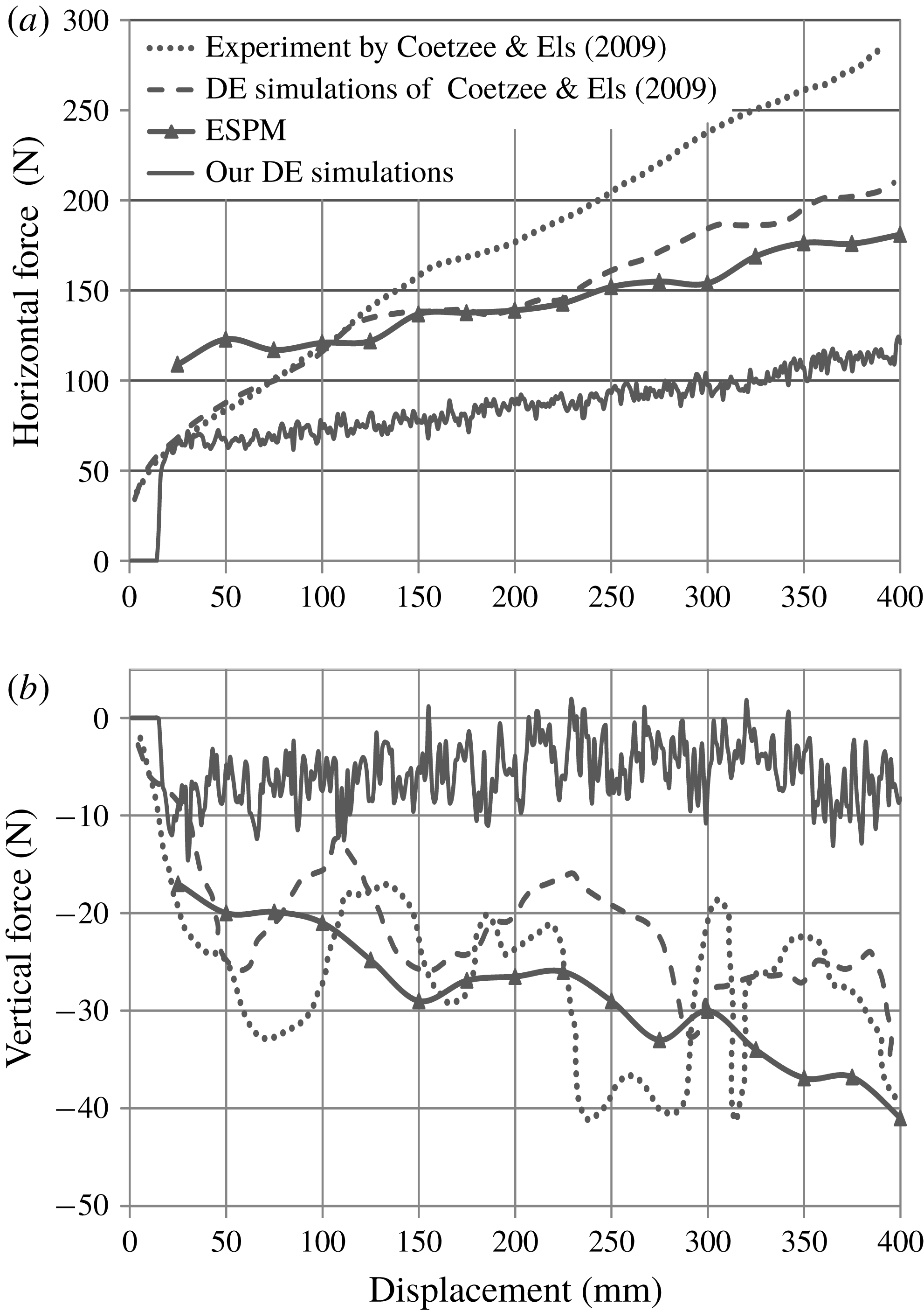
Comparing estimates for forces on the plough employed in the experiments of Coetzee & Els (Reference Coetzee and Els2009). Also shown are results from our two-dimensional simulations and those of Coetzee & Els (Reference Coetzee and Els2009), as well as predictions of ESPM. (a) Horizontal force. (b) Vertical force. Because the flow is developing, the transient time range is divided into finite time windows over which time averaging is done.

Coetzee & Els (Reference Coetzee and Els2009) performed experiments and two-dimensional DE simulations for a vertical plough cutting through a bed of corn grains. In their experiments: the vertical plough had an initial depth of 200 mm and width of 200 mm; the measured internal friction angle was
 $23^{\circ }$
; the calibrated microscopic grain properties yielded a grain density of
 $855~\text{kg}~\text{m}^{-3}$
, inter-grain friction coefficient
 $\unicode[STIX]{x1D707}_{p}$
of 0.12 and contact spring stiffness
 $k_{n}$
of
 $450~\text{kN}~\text{m}^{-1}$
. Coetzee & Els (Reference Coetzee and Els2009) used calibrated data in their DE simulations.
To apply ESPM we performed DE simulations using uncalibrated data shown in table 1, with grain friction coefficient
 $\unicode[STIX]{x1D707}=0.12$
. Another major difference between the DE simulations of Coetzee and Els and ours is that the former used clumped grains to imitate the shape of the corn grains, whereas we employ non-rotating, disc-shaped grains. The differences in the two DE simulations are reflected in figure 20, where we see that the two simulations predict very different ploughing forces. We discuss this further below.
In figure 20, we show the ploughing force measured by Coetzee & Els (Reference Coetzee and Els2009) in their experiments and computed by their calibrated two-dimensional DE simulations, the predictions of our uncalibrated two-dimensional DE simulations and, finally, the results of two-dimensional ESPM obtained after setting
 $\unicode[STIX]{x1D711}=23^{\circ }$
to match the bulk internal friction angle measured by Coetzee & Els (Reference Coetzee and Els2009). We see that ploughing forces predicted from the calibrated two-dimensional DE simulation and our ESPM are less than what is experimentally measured. This is because frictional forces exerted by the side walls in the experiments are not included in both two-dimensional DE simulations and ESPM. However, forces from the ESPM calculation come close to those predicted by calibrated DE simulations. This match is to be expected because the DE simulations of Coetzee & Els (Reference Coetzee and Els2009) utilized grain data calibrated to match the bulk internal friction angle
 $\unicode[STIX]{x1D711}$
of corn grains, and our ESPM, which employs the rheology of § 5.1, relies only on this choice of
 $\unicode[STIX]{x1D711}$
.
Figure 20 also plots predictions of our uncalibrated two-dimensional DE simulations that provided the kinematic data for our ESPM calculations. Forces predicted directly from our DE simulations, which employed disc-shaped grains, were less than those of all other predictions shown in figure 20, including the calibrated DE simulations of Coetzee & Els (Reference Coetzee and Els2009). This is because our DE simulations employ circular discs whose frictional properties were not tuned to capture the frictional interaction between corn grains. This underlines the importance of calibrating DE simulations to the actual macro-properties of the soil whenever force data are sought directly from DE simulations.
We saw in § 4.3 that ploughing is strain controlled to a great extent. Strain rates during ploughing are, therefore, largely insensitive to grain properties utilized in DE simulations. Thus, clumped grains employed by Coetzee & Els (Reference Coetzee and Els2009) in their DE simulations flowed in a manner very similar to our disc-shaped grains. Indeed, the maximum vertical displacement seen in our uncalibrated DE simulations was 142 mm, which is very close to the 145 mm peak displacement found by Coetzee and Els in their calibrated simulations. This explains the agreement of our ESPM calculations with the DE simulations of Coetzee and Els, even though the ESPM calculations utilized the strain field from our uncalibrated DE simulations. The fact that we obtained a good prediction from ESPM (i) without the extensive effort required to tune DE simulations and (ii) while using simple disc-shaped grains rather than the complex clumped grains of Coetzee and Els underscores the main advantages of ESPM.
6.2.2 Steel balls
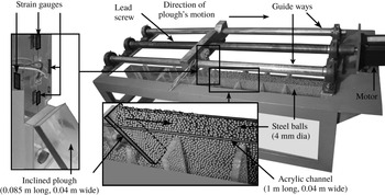
Experimental set-up to measure the ploughing force when a rigid, flat, inclined plough moves through a bed of steel balls.

Finally, we compare ESPM results with our experiments in which a rigid, flat, inclined plough made of acrylic ploughs through a bed of steel balls. The system is shown in figure 21. The length and width of the channel are 1 m and 40 mm, respectively, and the depth of the plough’s cut is 70 mm. The bed is a mixture of steel balls having diameters of either 4 or 3 mm. The inclination angle of the plough is kept at
 $50^{\circ }$
. The plough is mounted with a load cell consisting of strain gauges that are used for measuring horizontal and vertical forces. The lead screw with pitch length of 2 mm is driven by a stepper motor. The plough is attached to the lead screw that travels along two guideways on either side. The plough moves at speeds between
 $1$
and
 $18~\text{mm}~\text{s}^{-1}$
. Due to the limitation of the pitch length of the lead screw, we were unable to perform experiments over the entire range of speeds covered by simulations and ESPM. Only a small amount of surcharge accumulates (lower inset of figure 21) as the steel balls spill over the channel’s sidewalls. The channel is made of acrylic so that the friction of the walls with the steel balls may be ignored. Finally, we estimated the internal friction angle of an aggregate of steel balls to be
 $21^{\circ }$
by measuring the angle of repose of a heap of steel balls.
Kinematic data were obtained from uncalibrated DE simulations that employed parameters from table 1 and then following the process of §§ 4.1 and 4.2. In ESPM calculations the effective bulk density is taken to be
 $4830~\text{kg}~\text{m}^{-3}$
to match the density of steel times the volume fraction of 0.615 observed in DE simulations.
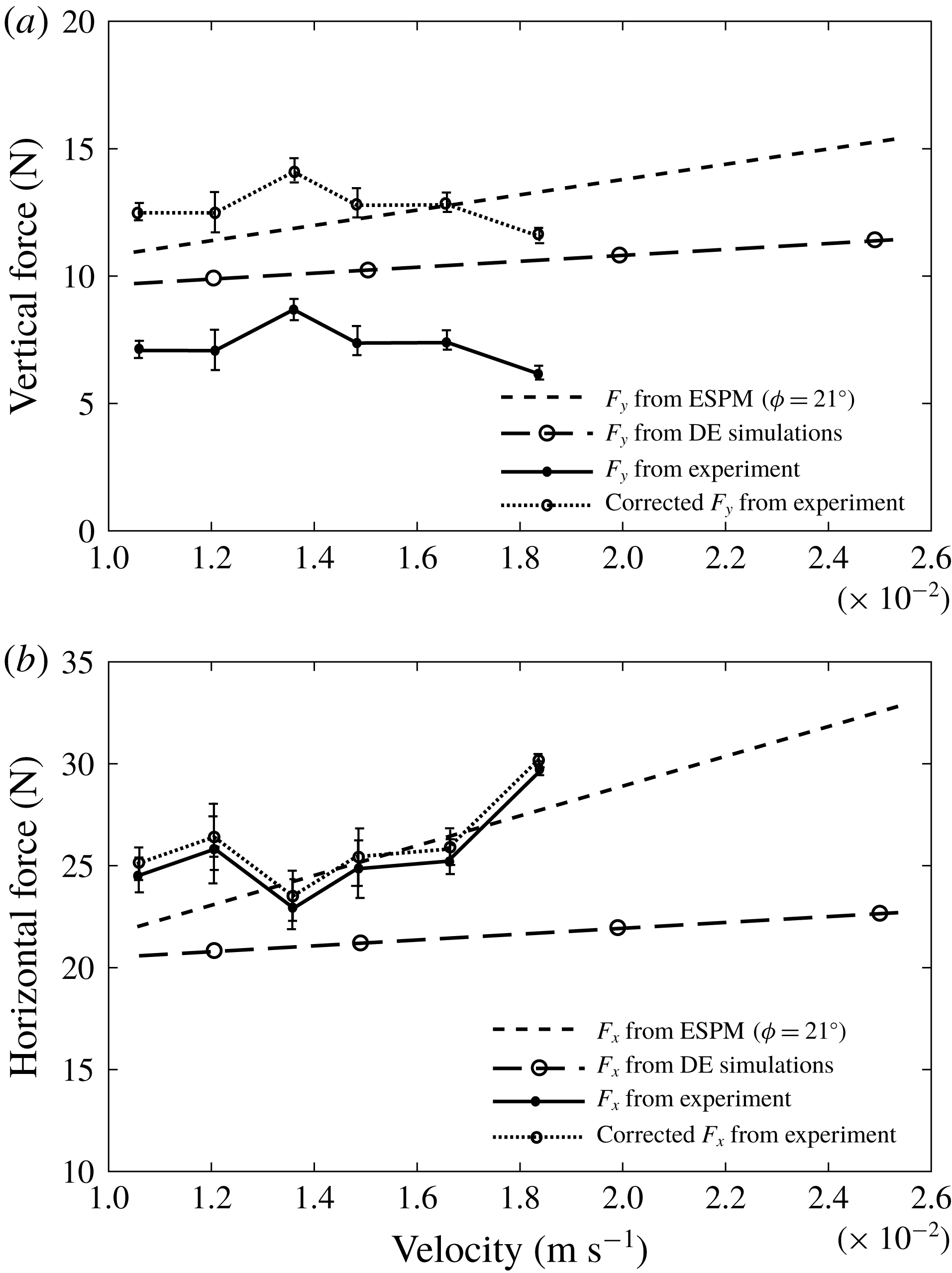
Figure 22 shows a comparison of the experiments with uncalibrated DE simulations and ESPM results. As expected, force predictions from DE simulations do not match experiments well. At the same time, the horizontal force measured from experiments is in good agreement with that predicted by ESPM. The vertical force found from ESPM, however, is higher than that measured in experiments. The absence of surcharge (lower inset of figure 21) and the presence of sidewall friction in our experiments are possible sources of this difference, as we show next.
Comparison of horizontal and vertical forces on the plough for the experiments of figure 21. (a) Vertical force (
 $F_{y}$
). (b) Horizontal force (
 $F_{x}$
).

The vertical force on the plough is affected only by the surcharge. However, the horizontal force is impacted by both the surcharge and the sidewall friction. Consider first the effect of the surcharge. From the universal earth-moving equation (McKyes Reference McKyes1985), the contribution of the surcharge to force normal to the plough is estimated using
 $$\begin{eqnarray}F_{sur}^{n}=q_{s}HN_{s}w,\end{eqnarray}$$
where
 $q_{s}$
is the lithostatic surcharge pressure,
 $H$
is the ploughing depth,
 $N_{s}$
is the surcharge factor that depends on the plough’s geometry and friction angle of granular material and
 $w$
is the plough’s width. From our DE simulations, the average height of surcharge above the plough is approximately
 $H/2$
and, hence, surcharge pressure
 $q_{s}=\unicode[STIX]{x1D70C}gH/2$
. The surcharge factor
 $N_{s}$
for a plough with inclination angle
 $\unicode[STIX]{x1D6FC}=50^{\circ }$
and a granular material with friction angle
 $\unicode[STIX]{x1D711}\approx 21^{\circ }$
is 1.61 (McKyes Reference McKyes1985, App. 1, p. 167). With this,
 $F_{sur}^{n}$
is found to be 7.48 N for our experiments. At the same time, the tangential force
 $F_{sur}^{t}$
on the plough’s surface due to the excess normal force
 $F_{sur}^{n}$
is
 $$\begin{eqnarray}F_{sur}^{t}=\unicode[STIX]{x1D707}_{as}F_{sur}^{n},\end{eqnarray}$$
where
 $\unicode[STIX]{x1D707}_{as}=0.15$
is the coefficient of dynamic friction between acrylic and dry steel. The corrected experimental measurements for the vertical force on the plough, obtained by adding the vertical components of
 $F_{sur}^{n}$
and
 $F_{sur}^{t}$
to the experimental values, are also shown in figure 22(a). We now find a good match between experiment and ESPM.
Correcting the experimentally measured horizontal force is more involved. The horizontal force should be first augmented by the horizontal components of
 $F_{sur}^{n}$
and
 $F_{sur}^{t}$
. At the same time, the contribution of the sidewall friction in experiments needs to be subtracted from the value of the horizontal force measured in experiments. We estimate the frictional force exerted by the sidewalls in our experiments by
 $$\begin{eqnarray}F_{sw}^{t}=\unicode[STIX]{x1D707}_{as}P_{sw}A_{sw},\end{eqnarray}$$
where
 $A_{sw}=l_{f}H$
is the sidewall area over which the friction force acts and
 $P_{sw}$
is the normal traction exerted by the grains on the sidewall. The traction
 $P_{sw}$
is estimated by
 $$\begin{eqnarray}P_{sw}=K_{0}F_{H}/A_{cs},\end{eqnarray}$$
where the at-rest earth pressure coefficient
 $K_{0}=(1-\sin \unicode[STIX]{x1D711})\approx 0.64$
(McKyes Reference McKyes1985),
 $A_{cs}=Hw$
is the cross-sectional area of the channel and
 $F_{H}$
is the measured horizontal force. The length
 $l_{f}$
over which the sidewall friction is mobilized is considered to be of the order of plough’s width
 $w=0.04$
m. This estimate is also consistent with the experiments of Tanaka et al. (Reference Tanaka, Momozu, Oida and Yamazaki2000) and Asaf et al. (Reference Asaf, Rubinstein and Shmulevich2007) which had plough velocities in the same range as in our experiments. The corrected horizontal force is plotted using dashed lines in figure 22(b), and is observed to be slightly higher than the value originally measured. The good agreement between experiments and ESPM nevertheless persists.
Finally, we note that in our ESPM computations we have ignored the contribution of frictional interaction between the granular flow and the aft side of the plough. This is because (i) we expect the normal force exerted by the grains on the aft side of the plough to be small, given that the granular flow has a free surface just beyond the plough, i.e. for
 $x<0$
, and (ii) the plough’s thickness is small.
7 Conclusions
The main objective of the paper was to demonstrate that we can calculate forces during ploughing of a granular bed by combining a continuum model of the granular flow with kinematic information obtained from uncalibrated DE simulations. Discrete element simulations can yield reliable force data only if they are first calibrated and if the number of grains is large enough. Calibration requires significant effort and is often system specific. Our method, which we label as the ESPM, obviates the need to calibrate DE simulations and also required far fewer grains.
The ESPM is useful for granular flows that are strain controlled, i.e. the strain field in the granular medium remains largely independent of grain properties such as shape, size and surface roughness. To this end we probed through DE simulations the extent to which ploughing is strain controlled and concluded that, for small enough grains, ploughing is strain controlled to a fair approximation. This allowed us to compute the strain field from coarse, uncalibrated, but representative DE simulations. The strain field was then combined with a rheology for flowing granular material and linear momentum balance to yield estimates for the ploughing forces. We selected a simple constitutive description to minimize the number of fitting parameters.
Ploughing forces were computed for a range of plough velocities. We saw that inertial effects played a negligible role at low velocities, but dominated at high velocities. Results from ESPM compared well with studies of Coetzee & Els (Reference Coetzee and Els2009) and Obermayr et al. (Reference Obermayr, Dressler, Vrettos and Eberhard2011). Although our DE simulations that fed into ESPM were uncalibrated and employed circular grains, as opposed to the complex clumped grains utilized by Coetzee & Els (Reference Coetzee and Els2009) in their calibrated DE simulations, forces predicted by ESPM showed a good match. Our own experiments were also in excellent agreement with ESPM results.
The present work may be augmented in several ways. The study was limited to two dimensions, but can be extended to three dimensions. Here, we utilized a simple constitutive model for the flowing grains as a first step. More comprehensive rheological models can lead to better results. Finally, only cohesionless grains are considered here. To address ploughing in cohesive granular media cohesion will have to be included in DE simulations that provide kinematic data to ESPM.
Acknowledgements
We thank Dr Ashish Bhateja (IIT Goa) for help with DE simulations and Shri Satya Prakash Mishra and Shri Amit Gaur for help with our experiments. S.M. and P.S. thank the Ministry for Human Resource and Development, Government of India for financial help through student scholarship. I.S. thanks Dr Kiran Akella (R&D Engineers, Pune) for bringing to our notice the problem addressed in this paper.
Appendix A. Effect of grid size
Figure 23 shows the variation in the components of strain rates when the size of the grid in figure 4 is modified. We observe that the change in the strain rates is small when the grid size is decreased from 0.5 to 0.25 non-dimensional units. Thus, we employ a grid size of 0.5 non-dimensional units to find the continuum velocity field
 $\boldsymbol{V}(x,y,t)$
associated with the ploughed granular material.
Components of the strain rate tensor at points along the line
 $y=9$
with different grid sizes. The tip of the plough is at
 $x=0$
. (a) Normal strain rate
 $\unicode[STIX]{x1D60B}_{xx}$
. (b) Normal strain rate
 $\unicode[STIX]{x1D60B}_{yy}$
. (c) Shear strain rate
 $\unicode[STIX]{x1D60B}_{xy}$
. The plough’s non-dimensional speed
 $v_{c}=10$
, the inter-grain friction
 $\unicode[STIX]{x1D707}=0.3$
and grain diameter
 $d=0.67$
.

Appendix B. Granular flow down an inclined plane
Here we investigate the flow of grains down an inclined plane and compare the predictions of ESPM with direct DE simulations and theoretical estimates obtained from the
 $\unicode[STIX]{x1D707}(I)$
-rheology (MiDi Reference MiDi2004). The
 $\unicode[STIX]{x1D707}(I)$
-rheology assumes that shear stress depends only on the local shear rate and is expressed in terms of friction coefficient
 $\unicode[STIX]{x1D707}$
and volume fraction
 $\unicode[STIX]{x1D719}$
depending on a single dimensionless number – the inertial number
 $I$
. Jop et al. (Reference Jop, Forterre and Pouliquen2006) utilized this rheology to put forward a three-dimensional, viscoplastic description of granular flow. Employing the
 $\unicode[STIX]{x1D707}(I)$
-rheology in the steady uniform regime for granular flow down an inclined plane, Pouliquen & Forterre (Reference Pouliquen and Forterre2009) found the normal stress
 $P$
and shear stress
 $\unicode[STIX]{x1D70F}$
to be, respectively,
 $$\begin{eqnarray}P(z)=\unicode[STIX]{x1D70C}_{p}\unicode[STIX]{x1D719}g\cos \unicode[STIX]{x1D703}(h-z)\quad \text{and}\quad \unicode[STIX]{x1D70F}(z)=\unicode[STIX]{x1D70C}_{p}\unicode[STIX]{x1D719}g\sin \unicode[STIX]{x1D703}(h-z),\end{eqnarray}$$
where
 $\unicode[STIX]{x1D703}$
is the inclination angle of the plane,
 $h$
is thickness of the flow in the
 $z$
direction and
 $\unicode[STIX]{x1D719}$
is the volume fraction, which was shown to be an unknown constant through the flow’s depth. The velocity profile
 $u(z)$
was found to be the Bagnold profile:
 $$\begin{eqnarray}u(z)=I(\tan \unicode[STIX]{x1D703})\frac{2}{3}\frac{\sqrt{\unicode[STIX]{x1D719}g\cos \unicode[STIX]{x1D703}}}{d}\{h^{3/2}-(h-z)^{3/2}\},\end{eqnarray}$$
which requires a knowledge of the inertial number
 $I$
.
To apply ESPM, we perform two-dimensional DE simulations considering a system of polydispersed, steady granular flows with 2100 grains. The length
 $l$
of the base and the thickness
 $h$
of the flow are, respectively,
 $20d$
and
 $100d$
, where
 $d$
is the diameter of the larger grain. The base is inclined at an angle
 $\unicode[STIX]{x1D703}=22^{\circ }$
, and this corresponds to flows that fall within the regime in which the constitutive law of § 5.1 is applicable. Our DE simulations will provide kinematic information to be utilized in subsequent ESPM calculations.
Our DE simulations parallel the L2 model of Silbert et al. (Reference Silbert, Ertaş, Grest, Halsey, Levine and Plimpton2001), with the following differences: (i) we use a smoother base, (ii) tangential springs are absent and (iii) the coefficient of restitution is lower (0.82 instead of 0.92). Figure 24(a) shows the velocity profiles obtained from our DE simulations and those of Silbert et al. (Reference Silbert, Ertaş, Grest, Halsey, Levine and Plimpton2001). We find a higher velocity near the base than that of Silbert et al. (Reference Silbert, Ertaş, Grest, Halsey, Levine and Plimpton2001) because we use a smoother base, while the greater grain inelasticity in our simulations is probably responsible for the reduction in velocity at the top of the flow. Nevertheless, our velocity profile agrees well with Silbert et al. (Reference Silbert, Ertaş, Grest, Halsey, Levine and Plimpton2001), and matches the Bagnold profile. We are unable to utilize the velocity profile (B 2) for comparison, because this requires knowledge of the inertial number for two-dimensional inclined plane flows, which is unavailable.
The volume fraction
 $\unicode[STIX]{x1D719}$
found from DE simulations is shown in figure 24(b), and again a close match is observed between our results and those of Silbert et al. (Reference Silbert, Ertaş, Grest, Halsey, Levine and Plimpton2001). Theoretically, Pouliquen & Forterre (Reference Pouliquen and Forterre2009) predict that the volume fraction is constant through the bulk, although the volume fraction itself was not predicted, and is found from experiments or simulations. This prediction matches simulations except near the top and bottom of the flow. The discussion so far confirms the correctness of the kinematics predicted by our DE simulations.
Comparison of (a) velocity and (b) volume fraction profiles obtained from our DE simulations and those of Silbert et al. (Reference Silbert, Ertaş, Grest, Halsey, Levine and Plimpton2001).

Now, we utilize ESPM to find the normal and shear stress, and compare with theoretical predictions (Pouliquen & Forterre Reference Pouliquen and Forterre2009) and direct DE simulations (Silbert et al.
Reference Silbert, Ertaş, Grest, Halsey, Levine and Plimpton2001). Both we and Silbert et al. (Reference Silbert, Ertaş, Grest, Halsey, Levine and Plimpton2001) find the bulk volume fraction
 $\unicode[STIX]{x1D719}$
to be approximately equal to 0.76. This estimate of the volume fraction will be utilized in (B 1). Figure 25 compares the stresses obtained by employing ESPM (using the deformation field from our DE simulations) with those found from the direct DE simulations of Silbert et al. (Reference Silbert, Ertaş, Grest, Halsey, Levine and Plimpton2001), and from the
 $\unicode[STIX]{x1D707}(I)$
-rheology. We find a good quantitative agreement between the direct DE simulations of Silbert et al. (Reference Silbert, Ertaş, Grest, Halsey, Levine and Plimpton2001) and ESPM. The manner in which the base is modelled in DE simulations is perhaps the reason behind the observed mismatch, especially in the shear stress in figure 25(b). The
 $\unicode[STIX]{x1D707}(I)$
-rheology tends to under-predict both normal and shear stresses, but the match is still reasonable.
Comparison of stress fields. (a) Normal stress and (b) shear stress. For
 $\unicode[STIX]{x1D707}(I)$
-rheology, we used
 $\unicode[STIX]{x1D719}=0.76$
, obtained from simulations.

The above analysis demonstrates the ability of ESPM to recover theoretical and direct computational results in the context of a well-studied granular system.