1. INTRODUCTION
In the last decades, an intense effort has been devoted to seeking a source of relatively clean and cheap energy, which can be in principle reached by the inertial confinement fusion. A small target containing a fuel must be compressed to a very high density and heated to a very high temperature owing to the very short confinement time, in order to ignite an efficient fusion burn. During the compression, a strong electromagnetic wave (EMW) usually interacts with a long rarefied plasma on a ns time scale. The indirect drive with its long scale-length plasma at the light entrance holes of hohlraum is the first example as described in Lindl (Reference Lindl1995). The other one is the direct drive, where it has been proposed to separate the process of fuel compression and ignition. A lower energy driver is then necessary for the fuel compression and the energy for the hot spot ignition is transported via energetic particles as in the fast ignition scheme or with a strong shock generated by a sudden jump in the heating beam intensity in a novel concept of the so-called shock ignition (Betti et al., Reference Betti, Zhou, Anderson, Perkins, Theobald and Solodov2007). However, the compressed target is surrounded by an expanding plasma corona, through which the heating beams are forced to pass, while the efficient transport and absorption of the incoming energy are crucial; but the energy transport from the beams to the target is influenced by various kinds of scattering phenomena accompanying the passage of the intense beams through the plasma corona, mostly in a non-linear stage. These phenomena are responsible for a significant incoming energy loss, a part of which is backscattered as an EMW or it is consumed by a hot electron generation.
One of these phenomena is the stimulated Raman scattering (SRS), which can be characterized as a resonant decay of incident laser light into a scattered EMW and an electron plasma wave (EPW). In one dimension (1D), we can distinguish two possibilities, Raman forward scattering and backscattering (SRBS) according to the propagation direction of the scattered EMW. Besides the energy loss by the backscattered EMW, the production of hot electrons in the high-amplitude electrostatic wave can play an important role during the fuel ignition. From this point of view, a deeper comprehension of this physical mechanism is necessary.
A complex numerical simulation of such a process is usually computationally demanding, so it is often replaced by a simpler computational model. The simplest model is the method of coupled mode equations (CME), where the amplitude of resonant wave modes are tracked in an approximation of slowly changing wave envelopes. The main problem of this method is that it does not take into account non-linear kinetic effects connected with the particle trapping in the EPW. The probably most popular method nowadays is the Particle-in-Cell method. It is capable of simulating larger systems even in higher dimensionality, but this method suffers from relatively high noise, which can hide fine details in the phase space. These details can, on the other hand, play an important role in the system evolution. The only method describing fine effects accurately is the Vlasov method solving the Vlasov equation for the distribution function together with an appropriate set of Maxwell's equations (Vlasov–Maxwell model).
There are several approaches how to solve the Vlasov equation. One of them is the Eulerian grid-based Vlasov solver, which comes from the ground-breaking paper of Cheng and Knorr (Reference Cheng and Knorr1976). This paper proposed a time-splitting scheme for the numerical solution of the Vlasov equation. As an example of a successful implementation of this method could serve the non-periodic code by Albrecht-Marc et al. (Reference Albrecht-Marc, Ghizzo, Johnston, Rveill, Sarto and Bertrand2007), which studied a saturation process of the SRBS in long scale-length underdense plasmas relevant to those which usually surround the fuel pellet in the laser fusion experiments. Another example is the work of Brunner and Valeo (Reference Brunner and Valeo2004), who observed the situation where the trapped particle instability revealed as a sideband growth of the EPW causes a bursting behavior of the SRS.
Our solution method for the full Vlasov–Maxwell system describing the SRBS will be that of Armstrong (Reference Armstrong1967). The resulting infinite set of ordinary differential equations for the time dependence of the unknown expansion coefficients of the Fourier–Hermite expansion scheme requires naturally a truncation to make the system finite. The truncation is a delicate operation, which might lead to a numerical failure of the solution for later times. However, we found that an addition of a small, but realistic collision term (Grant and Feix, Reference Grant and Feix1967) may rectify the situation and push the solution of the truncated system to later times, opening thus a possibility for a meaningful physical interpretation (Mašek and Rohlena, Reference Mašek and Rohlena2005). The numerical failure of the solution method is connected with the development of fine-scale structures on the distribution function. This requires a very high number of Hermite modes in late times of system evolution to guarantee the desired accuracy. The truncation of the Hermite expansion (setting a reflecting boundary condition) also causes the recurrence phenomenon where an incorrect information appears first at the highest Hermite modes and then it travels toward the lower Hermite modes destroying the whole calculation. Besides the simplified Fokker–Planck collision term mentioned in the text above, other ways how to slow down the spread of this incorrect information exist. Some authors use an artificial collision term to smooth the fine scale structures, but it distorts the distribution function in a non-physical manner [compare with Schumer and Holloway (Reference Schumer and Holloway1998)]. A detailed survey of these methods can be found in Section 2.3. A testing and benchmarking of several implementations of spectral methods applied to the non-linear Vlasov–Poisson equations can be found, for example, in Bourdiec et al. (Reference Bourdiec, de Vuyst and Jacquet2006); Parker and Dellar (Reference Parker and Dellar2015), and Camporeale et al. (Reference Camporeale, Delzanno, Bergen and Moulton2016). Moreover, first convergence studies and performance tests have been published for multidimensional Fourier–Hermite Vlasov solvers by Delzanno (Reference Delzanno2015) and Vencels et al. (Reference Vencels, Delzanno, Manzini, Markidis, Peng and Roytershteyn2016).
The aim of the present paper is to study the purely growing Raman instability and to visualize the competition between the collisional and the collisionless damping mechanisms of the daughter waves in the full kinetic situation. For this reason, the number of possible wave modes was kept at a moderate level reproducing essentially the system of interacting modes of the similar simplicity as it is usually considered by the CME (envelope equations) model, but with the full electron dynamic included in the simulation. The Fokker–Planck collision term stabilizes the method of numerical integration used in the model and at the same time it describes the electron–ion collisions in a natural manner. The detailed description of the used method can be found in Section 2. The detailed discussion of the physical results of such simulations, where we would like to assess the role played by the collisions in the particular physical situation is given in Section 3, where a special attention is also paid to the laser intensity dependence of the Raman reflectivity in Section 3.2 and to the influence of collisions on the temporal development of SRBS in Section 3.3.
2. VLASOV–MAXWELL CODE FOR THE STIMULATED RAMAN SCATTERING
We shall restrict ourselves to the non-relativistic plasmas generated by a ns laser pulse. This means that the dimensionless relativistic ratio
 $${\rm \theta} = \displaystyle{{v_{\rm T}} \over c} = \sqrt {\displaystyle{{K_{\rm B}T_{\rm e}} \over {m_{\rm e}c^2}}} ,$$
where
 $v_{\rm T} = \sqrt {K_{\rm B}T_{\rm e}/m_{\rm e}} $
is the thermal electron velocity, K
B is the Boltzmann constant, T
e is the electron temperature (later, in practical computations, the temperature will be specified by electronvolts, expressing thus the temperature in energy units), m
e is the electron mass, and c denotes the speed of light, must remain small, to be consistent. Moreover, we assume that the perpendicular motion of electrons is also non-relativistic. This implies the condition for the dimensionless parameter of laser pulse
 $$a_0 = \displaystyle{{eA_{\rm L}} \over {m_{\rm e}c}} \ll 1,$$
where e is the electron charge and A L is the amplitude of laser pulse. In such configurations, the electrons are accelerated solely by the longitudinal electric field, thus we can restrict ourselves to the 1D case and also we can replace the electron velocity in the perpendicular direction by the mean oscillatory velocity in the field of incident laser light:
 $$v_y = \displaystyle{{eA_y} \over {m_{\rm e}}}.$$
The vector potential has the only non-zero A
y
component in the perpendicular direction. This assumption is made mainly to keep the computational demand on a tolerable level, but we believe that it is a satisfactory assumption for the given physical situation. It is also useful to express the governing equations in a dimensionless form. In the non-relativistic case, it is natural to express the time in the units of reciprocal value of electron plasma frequency
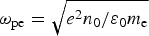 ${\rm \omega} _{{\rm pe}} = \sqrt {e^2n_0/{\rm \varepsilon} _0m_{\rm e}} $
where n
0 is the initial electron number density and ε0 is the permittivity of vacuum. The distance is compared to the Debye length
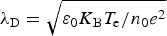 ${\rm \lambda} _{\rm D} = \sqrt {{\rm \varepsilon} _0K_{\rm B}T_{\rm e}/n_0e^2} $
where K
B is the Boltzmann constant and T
e denotes the electron temperature. Finally, the velocity scale is
 $v_{\rm T} = {\rm \omega} _{{\rm pe}}{\rm \lambda} _{\rm D} = \sqrt {K_{\rm B}T_{\rm e}/m_{\rm e}}. $
Our problem is 1D, there remains just a single meaningful dimension in the configuration space, which we designate as x, so that, for example, v x is the longitudinal component of velocity. Since it is impossible to confuse this longitudinal component of velocity v x with other components, the simplified notation v will be used in the following text. All quantities are taken from now on to be dimensionless.
The parametric instabilities are more likely to occur in a long scale-length plasmas, which allows a use of the homogeneous periodic model to study kinetic effects connected with the Raman scattering. The slow ion motion is negligible compared with the fast process of the Raman instability and the ions can be considered as an immobile neutralizing background, their (constant) number density must therefore be Zn
i = n
0 (ion charge is q
i = Ze). If we express the electromagnetic fields (E, B) in terms of their potentials (defined as
 ${\bf E} = - \partial {\rm \phi} /\partial x - \partial {\bf A}/\partial t,{\bf B} = \nabla \times {\bf A}$
) and use the Coulomb gauge (
 $\nabla \cdot {\bf A} = 0$
), we get the resulting dimensionless set of Maxwell's equations
 $$\left[ {\displaystyle{{\partial ^2} \over {\partial x^2}} - {\rm \theta} ^2\displaystyle{{\partial ^2} \over {\partial t^2}} - {\rm \theta} ^2\;n_{\rm e}} \right]A_y = 0,$$
 $$\displaystyle{{\partial ^2{\rm \phi}} \over {\partial x^2}} = n_{\rm e} - 1.$$
The electron number density n e is compared to its initial value n 0 and the vector and scalar potential is normalized to m e v T/e and K B T e/e, respectively. The dimensionless Vlasov equation for the electron distribution function f e takes the form
 $$\displaystyle{{\partial f_{\rm e}} \over {\partial t}} + v\displaystyle{{\partial f_{\rm e}} \over {\partial x}} + \left( {\displaystyle{{\partial {\rm \phi}} \over {\partial x}} - A_y\displaystyle{{\partial A_y} \over {\partial x}}} \right)\displaystyle{{\partial f_{\rm e}} \over {\partial v}} = 0,$$
where the relation (3) was used for the perpendicular component of velocity. The set of equations (4)–(6) is closed n e by means of the electron distribution function which is set as follows
 $$n_{\rm e} = \int\nolimits_{ - \infty} ^\infty {\,f_{\rm e}\;dv.} $$
2.1. Method of Solution
It is useful to consider a decomposition of the electron distribution function in the form f e(v, x, t) = f 0(v) + f(v, x, t), where f 0(v) is a spatially uniform distribution function satisfying
 $$1 = \int\nolimits_{ - \infty} ^\infty {\,f_0\;dv.} $$
The unperturbed quantity is used to preset the initial state of the plasma slab. The plasma in our model is initially in a statistical equilibrium characterized by the Maxwell distribution
 $$f_0 = \displaystyle{1 \over {\sqrt {2{\rm \pi}}}} e^{ - v^2/2},$$
which satisfies the condition (8). Using a corresponding decomposition for the electron density n e(x, t) = 1 + n(x, t) (the initial electron number density n 0 is taken as the unperturbed part), we get combining (7) and (8) for the perturbed part of electron distribution function:
 $$n = \int\nolimits_{ - \infty} ^\infty {\,f\;dv.} $$
The initial state of the vector potential is set by the decomposition A y (x, t) = A 0(x, t) + A(x, t), where the unperturbed part A 0 satisfies the wave equation in vacuum
 $$\left[ {\displaystyle{{\partial ^2} \over {\partial x^2}} - {\rm \theta} ^2\displaystyle{{\partial ^2} \over {\partial t^2}}} \right]A_0 = 0.$$
The unperturbed part of the vector potential then describes the pumping laser wave penetrating the plasma and is supposed to be A 0 = A Lcos(k L x − ωL t), which is also a solution of Eq. (11). Using the above decompositions, the Vlasov equation assumes the following form
 $$\displaystyle{{\partial f} \over {\partial t}} + v\displaystyle{{\partial f} \over {\partial x}} - F\displaystyle{{\partial f} \over {\partial v}} = F\displaystyle{{\partial f_0} \over {\partial v}} = - Fvf_0,$$
where F = (A 0 + A)∂ x (A 0 + A) − ∂ x ϕ. The Maxwell's equations are
 $$\left[ {\displaystyle{1 \over {{\rm \theta} ^2}}\displaystyle{{\partial ^2} \over {\partial x^2}} - \displaystyle{{\partial ^2} \over {\partial t^2}} - (1 + n)} \right]A = nA_0,$$
 $$\displaystyle{{\partial ^2{\rm \phi}} \over {\partial x^2}} = n.$$
2.2. Fourier–Hermite Expansion
We shall solve the Vlasov–Maxwell system (12)–(14) with the distribution function normalization (10) using a Fourier–Hermite transform method. This method is based on the Fourier expansion in the spatial coordinate x and the Hermite expansion in the velocity coordinate v. The use of Fourier expansion implies the periodic boundary conditions for our homogeneous plasma slab. In such a model, its spatial period L determines the smallest wave number k 0 = 2π/L. The period L must be tuned to accommodate the vectorial condition for the Raman scattering within our discrete k spectrum. The position of the pumping laser wave in the reciprocal space is then expressed as k L = j L k 0. This is reflected in the Fourier expansions of our quantities. For example, for the vector potential of electromagnetic field, the following expansion is used:
 $$A(x,t) = \sum\limits_{\,j = - \infty} ^\infty A_j(t)e^{ijk_0x},$$
and analogously for the scalar potential ϕ and the normalized electron number density n, which are coupled through Eqs. (10) and (14) with the electron distribution function, which is expanded in the following way:
 $$f\,(v,x,t) = \sum\limits_{\,j = - \infty} ^\infty \tilde f_j(v,t)e^{ijk_0x}.$$
Let us introduce the Hermite polynomials
 $$H_m(v) = \displaystyle{{{( - 1)}^m} \over {c_mw(v)}}\displaystyle{{{\rm d}^mw(v)} \over {{\rm d}v^m}},$$
where w(v) is a weight function and c m are normalization coefficients. The weight function should be continuous and positive such that the moments
 $${\rm \mu} _n = \int\nolimits_{ - \infty} ^\infty {w(v)v^n{\rm d}v} $$
exist for each n ≥ 0. In the present paper, we chose the weight function in the form
 $$w(v) = {\rm e}^{ - v^2/2}.$$
The main advantage of the use of such a weight function is its similarity with the equilibrium distribution function (9). The Hermite polynomials H m are orthogonal if employing the above-mentioned weight function in the definition of scalar product:
 $$\int\nolimits_{ - \infty} ^\infty {H_m(v)H_n(v)w(v) {\rm d}v = \displaystyle{{\sqrt {2{\rm \pi}} m!} \over {c_m^2}} {\rm \delta} _{mn}.} $$
The recurrence relations for Hermite polynomials are
 $$vH_m(v) = m\displaystyle{{c_{m - 1}} \over {c_m}}H_{m - 1}(v) + \displaystyle{{c_{m + 1}} \over {c_m}}H_{m + 1}(v),$$
 $$\displaystyle{d \over {dv}}H_m(v) = m\displaystyle{{c_{m - 1}} \over {c_m}}H_{m - 1}(v). $$
The choice of the normalization coefficients is arbitrary, but it is useful to define the Hermite polynomials as orthonormal, it means that from Eq. (20) we get
 $$c_m = (2{\rm \pi} )^{1/4}\sqrt {m!}. $$
Let us define an asymmetric set of Hermite functions
 $$h_m(v) = \displaystyle{{H_m(v)} \over {\sqrt {2{\rm \pi} m!}}} w(v), \, h^m(v) = \displaystyle{{H_m(v)} \over {\sqrt {m!}}}, $$
which makes a bi-orthonormal base in the infinite domain
 $$\int\nolimits_{ - \infty} ^\infty {h_m(v)h^n(v) \,\,\,dv = {\rm \delta} _{mn} \, {\rm for} \,m,n \ge 0.} $$
Each Hermite function satisfies velocity boundary condition h
m
(v) → 0 as v → ±∞ and they form an orthonormal basis of the Hilbert space of functions g(v) satisfying
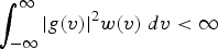 $\int_{ - \infty} ^\infty \vert g(v) \vert^2w(v)\;dv \lt \infty $
. The Fourier coefficients of the distribution function
 $\tilde f_j(v,t)$
are thus in addition expanded in a Hermite series:
 $$\eqalign{ {\tilde f}_j(v,t) & = \sum\limits_{m = 0}^\infty Z_{mj}(t)h_m(v), {\rm with} \cr Z_{mj} & = \int\nolimits_{ - \infty} ^\infty {{\tilde f}_j(v,t)h^m(v) dv.}} $$
Substituting these expansions into (12)–(14), the following infinite system of the first-order differential equations is obtained:
 $$\eqalign{ \displaystyle{{dZ_{mj}} \over {dt}} =& - ijk_0\left[ {\sqrt m Z_{m - 1,j} + \sqrt {m + 1} Z_{m + 1,j}} \right] \cr & - N_{mj} - \displaystyle{{{\rm \delta} _{m,1}} \over {\root 4 \of {2{\rm \pi}}}} F_j,} $$
 $$\displaystyle{{dA_j} \over {dt}} = - E_j,$$
 $$\eqalign{\displaystyle{{dE_j} \over {dt}} = & \bigg(1 + \displaystyle{{k_0^2 j^2} \over {{\rm \theta} ^2}}A_j \bigg) + R_j \cr & + \displaystyle{{\root 4 \of {2{\rm \pi}}} \over 2}[A_{\rm L}Z_{0,j - j_{\rm L}} + A_{\rm L}^* Z_{0,j + j_{\rm L}}].} $$
We denote the expansion coefficients of the transverse component of the electric field as E
j
. The expansion of the force term in the Vlasov equation is expressed as [
 ${{\rm \cal A}}(t) = A_{\rm L}\exp ( - i{\rm \omega} _{\rm L}t)$
]
 $$\eqalign{ F_j = &\displaystyle{{ij_{\rm L}k_0} \over 4}[{{\rm \cal A}}^2{\rm \delta} _{\,j,2j_{\rm L}} - {{\rm \cal A}}^{\ast 2} {\rm \delta} _{\,j, - 2j_{\rm L}}] \cr & + \displaystyle{{ijk_0} \over 2}[A_{\,j - j_{\rm L}}{{\rm \cal A}} + A_{\,j + j_{\rm L}}{{\rm \cal A}}^{\ast}] + Q_j + i\displaystyle{{\root 4 \of {2{\rm \pi}}} \over {\,jk_0}}Z_{0,j},} $$
and the convolution terms are
 $$N_{mj} = \sqrt m \sum\limits_{q = - \infty} ^\infty F_{\,j - q}(t)Z_{m - 1,q}(t),$$
 $$Q_j = ik_0\sum\limits_{q = - \infty} ^\infty A_qqA_{\,j - q},$$
 $$R_j = \root 4 \of {2{\rm \pi}} \sum\limits_{q = - \infty} ^\infty Z_{0,j - q}A_q.$$
Equations (27–29) form the infinite set of the first-order ordinary differential equations for the time-dependent expansion coefficients. It means that this set must be truncated before it can be numerically solved. The main issue of the transform method is the recurrence phenomenon or the numerical echo arising due to the truncation of the expansion. A detail discussion of a possible solution of this problem is a subject of the next subsection. The numerical integration of the set of differential equations is very sensitive to the integration time step, which is determined by the inverse of the highest frequency present in the simulation. One has to be very careful in the correct choice of its value if an explicit integration method is used. For that reason, we employed the implicit multistep Adams–Moulton method. The implicit method is able to handle the dense matrices associated with the truncated system attaining a good accuracy with no excessive computer time consumption.
One of the advantages of the transform method is that it allows one to apply more realistic initial conditions in the form of low-level white noise, because the Vlasov–Maxwell method is noiseless. Moreover, the reciprocal space renders the temporal evolution of resonant wave modes as an immediate result of the simulation. In the present paper, we deliberately chose the option of the method to set the Fourier spectrum as sparse as possible in order to study the kinetic effects connected with the pure Raman resonant mode only and thus to study a system similar to that described by the CME but with all the kinetic effects retained in the model. A suitable choice of the Fourier spectrum is suggested by a simple estimate of the side mode frequency. This is roughly given by the bouncing period of the trapped electrons in the potential wells (minima) of the forward electrostatic daughter waves inherent to the Raman scattering (Kruer and Dawson, Reference Kruer and Dawson1969)
 $${\rm \omega} _{{\rm Bf}} = \sqrt {\displaystyle{{eE_{\rm B}k_{\rm B}} \over {m_{\rm e}}}}, $$
where E B and k B are the amplitude of the electric field and the wave number of the electrostatic daughter wave, respectively. The bouncing frequency must thus remain smaller than the step of the Fourier spectrum multiplied by the electron thermal velocity
 $${\rm \omega} _{{\rm Bf}} \lt k_0v_{\rm T}.$$
This condition excludes the trapped particle instability, simplifying thus the overall physics behind our model facilitating the interpretation of numerical results.
2.3. Numerical Stabilization of the Method
As it has been mentioned, the system of Eqs. (27–29) is infinite and must be truncated to obtain a finite set. The well-known feature of the Vlasov equation is that it generates steep gradients on the distribution function during the phase space evolution, so higher and higher Hermite modes are necessary for an accurate description of the distribution function. This effect is known as the ‘filamentation’ in the phase space. When the upper boundary of the truncated matrix is reached, the information is ‘reflected’ inward the matrix, which is caused by the terms in the bracket on the right-hand side of Eq. (27), and a physically incorrect information keeps spreading throughout the matrix. There are several methods how to slow down this effect and push the correct solution toward a later time. The oldest one is the use of Fokker–Planck collision term (Grant and Feix, Reference Grant and Feix1967):
 $$\left( {\displaystyle{{{\rm \delta} f_{\rm e}} \over {{\rm \delta} t}}} \right)_{{\rm ei}} = {\rm \nu} _{{\rm ei}}\left( {\displaystyle{{\partial (vf_{\rm e})} \over {\partial v}} + \lt v^2 \gt \displaystyle{{\partial ^2f_{\rm e}} \over {\partial v^2}}} \right),$$
where
 $${\rm \nu} _{{\rm ei}} = \displaystyle{{4(2{\rm \pi} )^{1/2}Z^2e^4n_{\rm i}\ln {\rm \Lambda}} \over {3\sqrt {m_{\rm e}} {(K_{\rm B}T_{\rm e})}^{3/2}}}$$
is the electron–ion collision frequency [see, e.g. Eliezer (Reference Eliezer2002)]. Z is in this expression the mean ion charge, ln Λ is the Coulomb logarithm, K B is the Boltzmann constant and T e denotes the electron temperature. Note that this collision term conserves the momentum and energy of the electrons alone, which corresponds to the infinite mass of the motionless ions, which is an inherent assumption underlying our SRBS theory. The collisional term tends to suppress the highest terms in the Hermite expansion, which remain after the truncation, and thus naturally improves the convergence of the scheme, which is impaired if these marginal terms remain too large. This would be contrary to the very idea of the truncation. Their suppression is marked by a smoothness of the distribution function in the interval of higher velocities. The same purpose is served by the interpolation schemes in the time-splitting methods solving the Vlasov equation on a grid in the configuration space (Cheng and Knorr, Reference Cheng and Knorr1976). We found this scheme as sufficiently stable for our study of the SRS in the weakly collisional laser corona, so we can benefit from the fact that the collisions are now added to the model in a natural way and therefore no non-physical entropy growth is experienced.
Naturally, other methods, how to stabilize the solution method, have been developed. Shoucri and Gagne (Reference Shoucri and Gagne1976) strengthen the selectiveness of the damping term in such a way that the higher expansion coefficients are damped even more efficiently. Another artificial collisional damping term was used by Camporeale et al. (Reference Camporeale, Delzanno, Bergen and Moulton2016). They artificially excluded the influence of Fokker–Planck collisional term on the first three coefficients of the Hermite expansion, so that the charge, momentum, and energy are conserved during the simulation. Joyce et al. (Reference Joyce, Knorr and Meier1971) use the fact that the spectrum exhibits a very regular pattern when the power transform is used. It is then possible to employ a polynomial extrapolation to find the missing coefficient above the edge of the truncated matrix. When the collisionless case of the Vlasov equation is to be studied, it is useful to use the velocity space analog of the spectral filter discussed by Hou and Li (Reference Hou and Li2007). This method of numerical stabilization was successfully used by Parker and Dellar (Reference Parker and Dellar2015) for a solution of Vlasov–Poisson model by the Fourier–Hermite transform method.
3. RESULTS OF NUMERICAL SIMULATION
In this contribution, it was our intention to extend the results of our previous work (Mašek and Rohlena, Reference Mašek and Rohlena2015) and look at the entire problem of the non-linear evolution of the system in a more detail. The goal is to study the influence of the collisions (and their competition with the collisionless damping mechanisms) on the development of the Raman instability and on the resulting reflectivity. To do this, we ran our code for several values of the laser intensity. Results for a fixed collision frequency are a subject of Section 3.2. To generalize those results we ran our code with a varying collision frequency and fixed laser intensity and other parameters. The results of such simulations are presented in Section 3.3.
3.1. Simulation Run Settings
We concentrated on two different cases of plasma configuration. The first one was inspired by the hydrodynamic simulations of the shock ignition experiment on the OMEGA facility Theobald et al. (Reference Theobald, Nora, Lafon, Casner, Ribeyre, Anderson, Betti, Delettrez, Frenje, Glebov, Gotchev, Hohenberger, Hu, Marshall, Meyerhofer, Sangster, Schurtz, Seka, Smalyuk, Stoeckl and Yaakobi2012). The resulting electron temperature of these simulations varied from K
B
T
e ≈ 1.6 keV in the less dense outer part of the plasma corona to K
B
T
e ≈ 2.1 keV in the regions lying closer to the quarter-critical density. Since we assume a homogeneous plasma in our simulations, we fixed the value of the electron temperature at K
B
T
e = 2 keV. Secondly, to generalize our results, we also ran our code for a higher temperature K
B
T
e = 5 keV, which can be expected in multi-beam laser facilities. Such plasmas are irradiated by laser pulses with the wavelength
 ${\rm \lambda} = 351{\kern 1pt} \;{\rm nm}$
.
We restricted our study to a few widely separated resonant wave modes by imposing a fairly sparse discrete Fourier spectrum to suppress the satellite modes and thus to study a purely growing Raman instability, in a similar way which is used in the CME models. This enabled us to conserve a relatively low number of the Fourier modes in the calculation. The position of the impinging laser wave in the reciprocal space was set to k L = 4 k 0. The value of the smallest wave number is determined from this assumption as k 0 = 2.96 × 10⁻² and the length of simulation box was thus L = 212.54. According to Eq. (35), this value of k 0 is large enough to suppress the sideband growth.
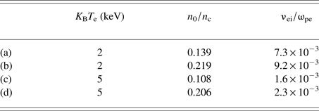
The use of such sparse discrete Fourier spectrum demands a fine tailoring of the value of the electron number density to fulfill the SRBS matching conditions together with zeroth-order dispersion relations for EPW and EMW within our discrete wave number spectrum. The electron–ion collision frequency was determined for each case as to simulate plasmas with the mean ion charge Z = 6. The simulation parameters are summarized in Table 1.
Summary of simulation parameters for the studied cases.

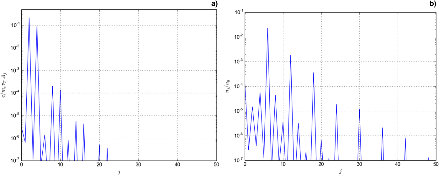
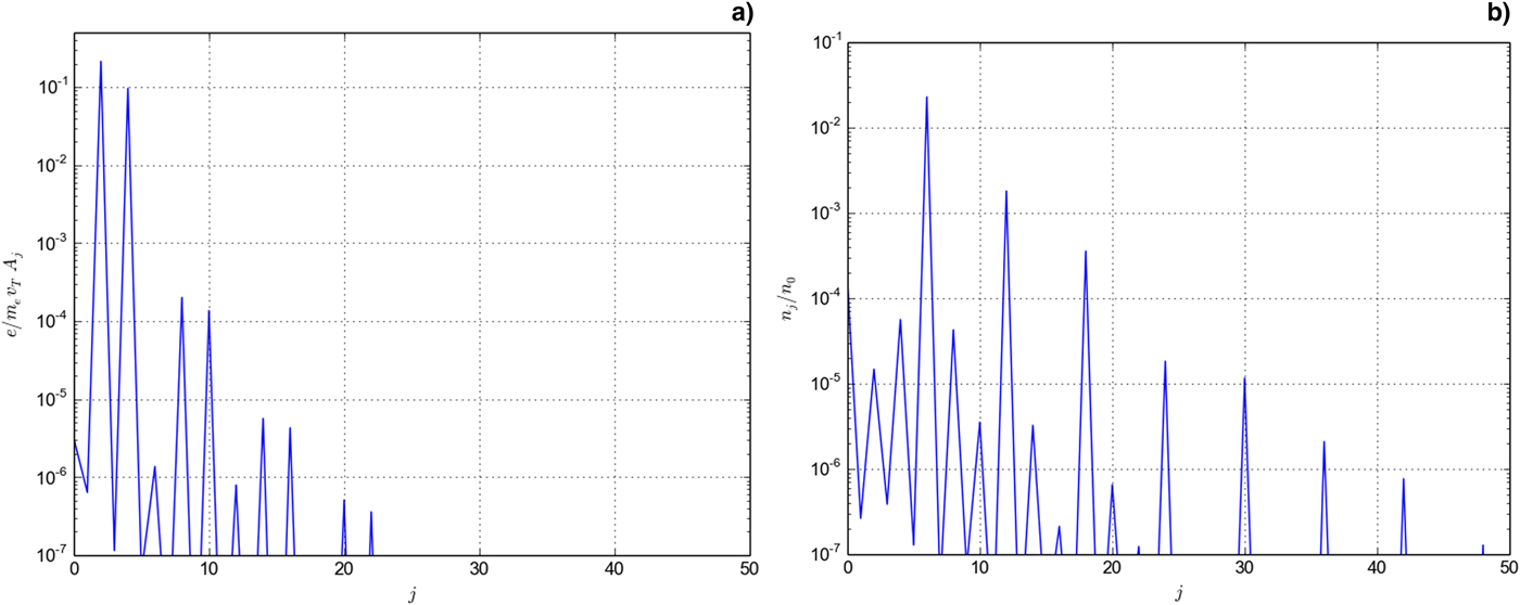
Since both the resonant wave modes lie in the spectrum below twice the wave number of the pumping wave, the Fourier series can be truncated with a relatively low maximum wave number, which was set in the present simulations to be k max = 50 k 0. The validity of this assumption is demonstrated in Figure 1, where the fully developed spectrum of electromagnetic and electrostatic wave modes from the simulation in case (a) at ωpe t = 800 are depicted. It is evident that the higher wave modes vanish quickly and do not interfere with the evolution of the system. The Hermite expansion is truncated after the first 400 terms, which ensures a good accuracy of the reconstructed distribution function. Moreover, together with our choice of the collision frequency, this value is sufficient for our purpose to slow down the recurrence phenomenon and thus reach the interesting stages of the system evolution.
Fully developed spectrum of (a) electromagnetic wave modes and (b) electrostatic wave modes at ωpe t = 800.
3.2. Intensity Dependence Study of the SRBS
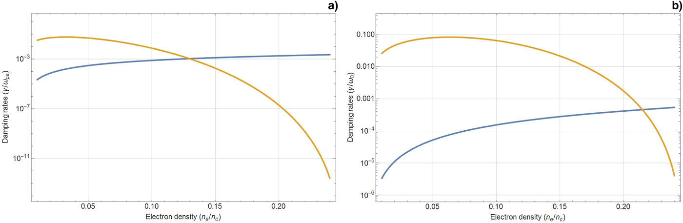
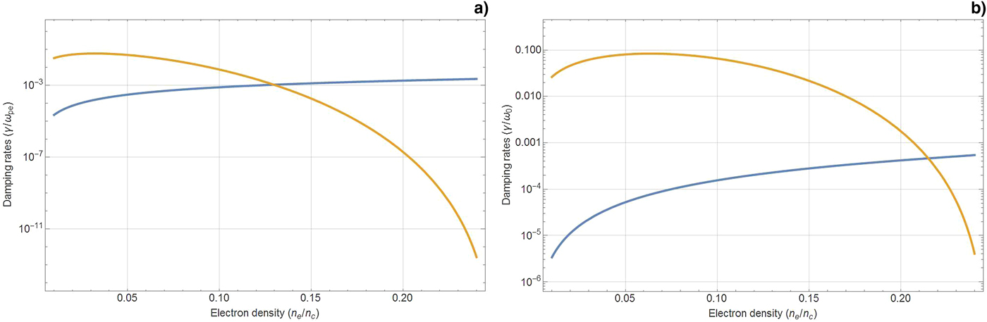
The kinetic Vlasov–Maxwell simulations showed that the collisional instability threshold is somewhat shifted toward higher laser intensities and the instability growth is somewhat lower as against the predictions of the linearized theory. Compared to the linearized theory, the shift is more significant in the lower density case (approximately by one order of magnitude) than in the denser plasma, where a much smaller shift was found. It can be explained with the help of Figure 2, where both the collisional (blue line) and Landau (orange line) damping rates are plotted as a function of electron number density in (a) 2 keV and (b) 5 keV plasmas. In the less dense plasma, the collisionless damping dominates over the collisional one while in the denser plasma the damping process is dominated by collisions. Since the Landau damping represents in the linearized theory the simplest kinetic effect, so especially in the parameter range where the Landau damping dominates the collisional damping, the inclusion of a more precise description of kinetic effects in the electron phase space will essentially modify the results of the linearized theory, the most significant being the presence of the trapped electrons in the kinetic model. This leads to the greater damping of the EPW and it results in an increase of the instability threshold and lowering of the instability growth rate. On the other hand, with the increasing laser intensity of the SRBS, the growth rate is approaching the value predicted by the linearized theory (with the linear Landau damping taken into account). This can be understood in terms of a very strong parametric growth rate ΓB (k B and ωB are wave number and frequency of the resonant EPW, respectively)
 $${\rm \Gamma} _{\rm B} = \displaystyle{{k_{\rm B}v_{{\rm osc}}} \over 4}\sqrt {\displaystyle{1 \over {{\rm \omega} _{\rm B}({\rm \omega} _{\rm L} - {\rm \omega} _{\rm B})}}}, $$
of the Raman instability (SRBS) occurring in this region, which invalidates both the collisional and collisionless damping mechanisms. In this case, the influence of the non-linear electron kinetics remains only marginal, and the CME envelope equations (with the linear Landau damping included) represent in this case a meaningful model.
EPW damping rates for (a) 2 keV and (b) 5 keV plasma as a function of electron number density. Landau damping rate γ L and collisional dampig rate γB are plotted using orange and blue lines, respectively.
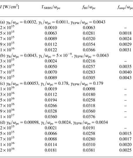
The wave amplitudes then continue to oscillate as the energy is exchanged between the electrostatic wave and the trapped particles, which is also obvious from the phase space picture. In these cases, the amplitude oscillations are caused mainly by both the collisional and the collisionless damping processes balanced by the instability growth, which is pumped by the incoming laser pulse. This is demonstrated by Table 2, where the theoretical and simulated values of characteristic frequencies are confronted. The collisional damping rate equals
 $${\rm \gamma} _{\rm B} = \displaystyle{{{\rm \omega} _{{\rm pe}}{\rm \nu} _{{\rm ei}}} \over {2{\rm \omega} _{\rm B}^2}}, $$
where ωB is the frequency of the electrostatic daughter wave. We evaluated the Landau damping rate γ L and also the total damping rate of the EPW γ EPW = γ B + γ L for each of the studied cases. The frequency of electron bouncing ωBf = 2πf Bf was defined by Eq. (34). The frequency of the EPW amplitude oscillations f amp obtained from the numerical results of Vlasov–Maxwell simulations is also shown. Another important parameter contained in Table 2 is the growth rate of Raman instability, when all the damping processes are taken into account on the basis of linear theory (Drake et al., Reference Drake, Kaw, Lee, Schmid, Liu and Rosenbluth1974):
 $${\rm \Gamma} _{{\rm SRBS}} = \displaystyle{1 \over 2}\left[ { - ({\rm \gamma} _{{\rm EPW}} + {\rm \gamma} _ - ) + \sqrt {{({\rm \gamma} _{{\rm EPW}} - {\rm \gamma} _ - )}^2 + 4{\rm \Gamma} _{\rm B}^2}} \right].$$
The relation (40) is valid for the weakly coupled regime, which means such a regime where the dispersion of the electrostatic wave is not influenced (or influenced just slightly) by the pumping electric field.
Characteristic frequencies for the studied plasma configurations with different laser intensities. The values are calculated for (a) n 0/n c = 0.139, K B T e = 2 keV, (b) n 0/n c = 0.219, K B T e = 2 keV, (c) n 0/n c = 0.108, K B T e = 5keV and (d) n 0/n c = 0.206, K B T e = 5 keV.

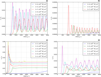
As it has been already mentioned, the damping processes are responsible for the amplitude oscillations while the motion of the trapped electrons causes just small and relatively fast amplitude modulations. Table 2 shows that the frequency of amplitude oscillations observed in the simulations f amp are significantly modified by the kinetic effects, though an order of magnitude difference compared to the total damping rate γ EPW of the EPW is mostly absent. In the cases of low laser intensity slightly above the instability threshold (Tables 2a, 2b and 2d), no significant oscillations were found, which indicates that the undamped instability growth (38) is not strong enough to compensate the damping and just a quasi-stationary state with low-level saturation of the EPW amplitude is reached. A similar situation was observed also in the case of less dense 5 keV plasma, where the phase velocity of the resonant EPW lies close to the body of electron distribution and a very strong collisionless damping is present. Then a fairly high number of electrons is quickly trapped in the EPW (see Fig. 3c). Since the instability growth rate is not high enough (compare Table 2) and the quasi-stationary state with the small amplitude fluctuations caused by the motion of the trapped electrons is established again with a dramatic reduction of reflectivity as against the expectations based on the linear theory or the CME model, where a very high instability growth and reflectivity are predicted. This quasi-stationary state can be perturbed only by the interference of an additional mode of EPW connected, for example, with the trapped particle instability or a different kind of decay instability (Brunner & Valeo, Reference Brunner and Valeo2004; Mašek & Rohlena, Reference Mašek and Rohlena2008).
Trapped electron number density for (a) n 0/n c = 0.139, K B T e = 2 keV, (b) n 0/n c = 0.219, K B T e = 2 keV, (c) n 0/n c = 0.108, K B T e = 5 keV and (d) n 0/n c = 0.206, K B T e = 5 keV.

The whole situation is further complicated by the trapped electrons, whose number and influence on the system evolution increases with the increasing EPW amplitude. See Figure 3, where the temporal dependence of the trapped electron number density is shown for all the studied cases. The trapped electrons structures are, however, disturbed by the collisions, when some electrons leave the trapping region and the EPW is no longer damped by the collisionless mechanism as before and its growth is restored. If there were no collisions present (or were negligible compared to the Landau damping), a different kind of equilibrium would be established as it is the case of Figure 3c, where the collision frequency is much lower than the Landau damping rate. The decrease in number of trapped particles and EPW damping reduction is, of course, caused also by the fact that the proportion of trapped electrons is decreasing with the decreasing EPW amplitude, as it is also visualized by the phase space picture, which means that the electron can leave the trapping regions also in this way. The competition of both the physical processes leads to the temporal dependence of the number density of trapped electrons, which is shown in Figure 3 for all the studied cases. It is easily seen from Figure 3b that even for a very low trapped electron number density (n trapped is of the order of 10−5 n 0), the system evolution is strongly influenced by these trapped particle structures in the phase space and the instability growth together with the resulting reflectivity is strongly reduced as compared to the result of CME model. In the other cases, where the proportion of trapped electrons amounts to a few percent of the initial electron number density, the influence on the system evolution is relatively high, as it is to be expected. In the lower density 5 keV case, where the EPW phase velocity lies close to the body of the initial electron distribution, the trapped electron number density, however, does not reach a significantly higher value (compare with Fig. 3c). This is caused by the fact that the instability development is in a strongly non-linear regime from the very beginning of the simulation and the EPW does not reach a sufficiently high amplitude to trap a significantly higher number of electrons. However, compared to the CME model, the instability development still behaves in a totally different manner.
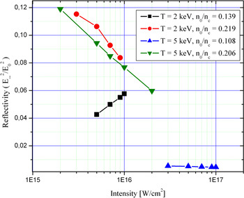
The purpose of this contribution was mainly to study the Raman reflectivity influenced by both the collisional and collisionless damping mechanism. Based on the discussion of the influence of both the damping mechanisms on the SRBS development and their competition as described in the previous text, the results of the Vlasov–Maxwell simulations can be best characterized by looking at the average values of resulting reflectivity dependence on the laser intensity as plotted in Figure 4. In the region of collisionless damping domination (K
BTe = 5keV, n
0/n
c = 0.108), a fast increase in reflectivity is observed following the onset of a stationary situation caused by the bouncing motion of the trapped electrons. We found no significant change in the resulting value of reflectivity (
 $R \approx 0.5\% $
) with the laser intensity. The reason is a strong non-linear ‘wave–particle’ interaction, which cannot be compensated by the (relatively high) instability growth, even if it is dramatically increasing with the laser intensity (compare with Table 2). When the phase velocity lies off the body of the distribution, the interplay between the collisional and the collisionless process leads to a reflectivity amplitude oscillations and no stationary state is reached. The increase in the Raman reflectivity with the increasing laser intensity was observed in the less dense 2 keV case. Here the influence of both the damping mechanisms is similar, but with the increasing laser intensity, the EPW amplitude reaches a higher value and thus it influences a larger region of the phase space (see Fig. 3), which, in turn, enhances the collisionless damping mechanisms. Collisional mechanisms are then not strong enough to damp the resonant waves and the resulting reflectivity is increasing. In contrast, the decrease in the reflectivity with the increasing laser intensity is observed in the denser plasma for both the cases of electron temperatures. From Figure 3, it is clear that less electrons are affected by the potential of EPW, in the case (b) is the proportion of trapped electrons lower by a few orders of magnitude. Here we are in the regime where the collisions are dominant, so that the EPW potential does not influence too many electrons for a longer time (EPW phase velocity is far away from initial electron distribution). This, in turn, permits the development of big regions of the trapped electrons in the phase space. These regions are larger for higher laser intensities and the collisionless damping gradually increases. This mechanism results in a Raman reflectivity decrease with the increasing laser intensity.
Laser intensity dependence of average Raman reflectivity in all the studied cases.

3.3. Collisionality Dependence Study of the SRBS
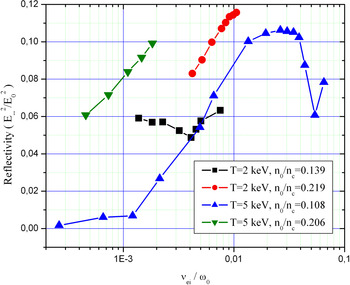
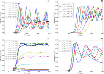
It is instrumental also to study the dependence of the instability behavior on the collision frequency. These studies are summarized in Figure 5, while the temporal evolution of the laser reflectivity in all the studied cases is shown in Figure 6. The increase in the reflectivity with the increasing collision frequency was observed in both the higher density cases. From Figure 6b and 6d, it is clearly visible that the EPW amplitude oscillations period is decreasing with the increasing collision frequency and the oscillations reach a lower amplitude with a larger average reflectivity. In the less dense 5 keV plasma, a limiting value of collision frequency with a maximum laser reflectivity was found. If the collision frequency is higher than this limiting value, the laser reflectivity goes down. In this situation, the collisional processes dominate over the collisionless ones and the system is strongly collisionally damped. The initial increase of reflectivity can then be understood using the same argument as in the text above. The collisional processes act against the collisionless damping mechanisms of the EPW, which in turn enables the wave amplitude to reach a higher saturation level. This observation is in agreement with the results of the paper Liu et al. (Reference Liu, Ping Zhu, Cao, Zheng, He and Wang2009) and the existence of such a limiting value can be expected also for the other cases. On the other hand, these values of collision frequency correspond to a very high plasma ionization. An exception from this behavior was observed in the less dense 2 keV case, where the reflectivity passes through a minimum followed by an increase in higher collision frequencies. In this case, the collisionless damping regime dominates for low collision frequencies. The turning point corresponds roughly to the value where both the damping rates are comparable. As it is seen in Figure 6a, the reflectivity amplitude oscillations are reduced with the increasing collision frequency and an almost constant value of reflectivity is reached in a steady state for the higher collision frequencies with the growing saturation level if collision frequency increases.
Collision frequency dependence of average reflectivity at fixed laser intensity I = 9 × 10¹⁶ W/cm2 in the less dense 5 keV case and at the intensity I = 9 × 10¹⁵ W/cm2 in all other cases.

Temporal evolution of reflectivity from the full Vlasov–Maxwell simulation at different collision frequencies for (a) n 0/n c = 0.139, KBTe = 2 keV, I = 9 × 10¹⁵ W/cm2, (b) n 0/n c = 0.219, KBTe = 2 keV, I = 9 × 10¹⁵ W/cm2, (c) n 0/n c = 0.108, KBTe = 5 keV, I = 9 × 10¹⁶ W/cm2, and (d) n 0/n c = 0.206, KBTe = 5 keV, I = 9 × 10¹⁵ W/cm2.

From what has been just said, it is obvious that the value of the collision frequency may influence the calculation outcome in a non-trivial way. It may even happen that an unnecessarily excessive value of the collision frequency may eradicate or hide interesting physical phenomena, which would otherwise turn up with a less collisional regime, without, however, losing the numerical benefits of the incorporation of the collision term as such.
4. CONCLUSION AND DISCUSSION
A Vlasov–Maxwell set of equations was solved for realistic conditions of a laser corona heated by a laser beam represented by a monochromatic plain wave of large amplitude. The solution restricted to 1D geometry was found using a transform method of a double expansion in a Hermite–Fourier series, which was subsequently truncated for the purpose of a systematic computer modeling. We found that the method is showing a reasonable numerical stability when including a small electron–ion collision term in the electron Vlasov equation. The ions were supposed to remain fixed in a homogeneous plasma of the laser corona. With these limitations, the most important non-linear process turns out to be the SRBS of the impinging wave on the plasma electrons, leading to a transformation of the primary laser wave to a backscattered wave and a forward propagating electrostatic electron plasma daughter wave (EPW). Such a process can in the simplest way be described by a system of coupled-mode equations describing the wave transformation satisfying the resonance conditions for both the frequencies and wave vectors of the participating waves. To exclude more complex wave transformation processes which are intrinsically present in the full kinetic model, we purposely kept the Fourier spectrum as sparse as possible, by which the results of the full kinetic solution could be easily interpreted as wave modes described by the CME. However, even in this very simplified situation thanks to the underlying electron kinetics the wave behavior becomes very different from a coupled mode solution (even if augmented by a linear Landau or collisional damping rates), with important consequences, for example, for the Raman reflectivity. The main difference is caused by the phenomenon of electron trapping. For a smaller amplitude of the laser field, the filling rate of the potential wells of EPW with the trapped electrons competes with the collision rate, which may knock out most of the trapped electrons out of the potential wells and thus a nearly linear regime is renewed till the trapping regions are filled again. Then the phenomenon repeats in the form of EPW amplitude oscillations. For a stronger laser field, the potential wells of EPW are deeper and the number of trapped electrons is higher, so that the collisions are no longer capable of emptying the potential minima entirely. This situation leads to an EPW amplitude saturation with the trapping rate balanced by the collision rate. This varying behavior of the trapped electron population influences strongly also the Raman reflectivity. The collisions are, however, not the only mechanism leading to a reduction of the trapped electron population. As already mentioned, the sparse Fourier spectrum imposed for a simplicity in our computational examples does not allow a growth of the satellite mode due to the trapped particle instability. If a denser Fourier spectrum were permitted, the satellite modes of EPW would emerge and their field would combine with the EPW own electric field. This additional field would also cause at least part of the trapped electrons to leave the potential wells, which in extreme cases may wipe out the EPW and thus the trapped electron population entirely. If this is the case, the Raman instability under the constant laser illumination starts to grow anew and the whole chain of events will be repeated. This is the underlying mechanism of a bursting behavior of the Raman instability also reported in Brunner and Valeo (Reference Brunner and Valeo2004) and in Mašek and Rohlena (Reference Mašek and Rohlena2010).
ACKNOWLEDGMENTS
Authors greatly appreciate a financial support from the Czech Ministry of Education, Youth and Sports (grant nr. LG15013 and LD14089). The access to computing and storage facilities owned by parties and projects contributing to the National Grid Infrastructure MetaCentrum, provided under the program ‘Projects of Large Infrastructure for Research, Development, and Innovations’ (LM2010005) is highly acknowledged.