





1 Introduction
Xiao–Zhu have raised a question on
$S=T$
 for Shimura varieties in [Reference Xiao and ZhuXZ17, Conjecture 7.3.13], which states that excursion operators on the compactly supported cohomology are the same as Hecke operators and is an analogue of Lafforgue’s
$S=T$
 theorem in [Reference LafforgueLaf18, Proposition 6.2]. This is a fundamental question that can be interpreted as a local-global compatibility in a categorical formulation of the Langlands correspondence, see [Reference ZhuZhu20, Conjecture 4.7.16]. Moreover, it has consequences for the Eichler–Shimura relation for compactly supported cohomology of Shimura varieties of Hodge type, see [Reference Xiao and ZhuXZ18, Proposition 6.3.1].
The main result of this paper is a proof of this conjecture.
Theorem 1.1. Let
$X_K$
 be a Shimura variety of Hodge type with respect to a reductive group G and level K. Let p be a prime over which G is unramified, and K is hyperspecial at p. Let l be a prime different from p. Then we have an identity

as endomorphisms of
$H^i_c(\mathfrak {X}_{K,\overline {\mathbb {F}_p}},\overline {\mathbb {Q}}_\ell )$
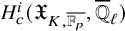 , where
$\mathfrak {X}_K$
 is the smooth integral model of
$X_K$
 constructed in [Reference KisinKis10], V is a representation of
$^L G$
 ,
$T_V$
 is the Hecke operator associated to V as defined in Section 4, and
$S_V$
 is the excursion operator associated to V as defined in [Reference Xiao and ZhuXZ17, Section 7.3.11].
An application of this result, as observed by Xiao–Zhu, is the generalization of the classical Eichler–Shimura relation ([Reference ShimuraGS58], [Reference EichlerEic54]) to Shimura varieties of Hodge type, proving a conjecture of Blasius–Rogawski in this setting.
Corollary 1.2. ([Reference Xiao and ZhuXZ18, Proposition 6.3.1])
We have the Eichler–Shimura relation for Shimura varieties of Hodge type.
Strictly speaking, there are two versions of
$S=T$
 in mixed characteristic (while there is only one in equal characteristic). The first is
$S=T$
 for moduli spaces of mixed characteristic shtukas, and the second is the one for Shimura varieties. In [Reference Xiao and ZhuXZ17], Xiao–Zhu have proved
$S=T$
 for moduli spaces of Witt vector shtukas (
$loc.cit.$
 theorem 6.0.1 (2)), and zero-dimensional Shimura varieties (
$loc.cit.$
 proposition 7.3.14). However, even their version for moduli spaces of shtukas is strictly weaker than Lafforgue’s
$S=T$
 theorem in equal characteristic and is again zero dimensional in nature. More precisely, they have proved that the excursion operator associated to a representation of the Langlands dual group acts on the cohomology of a zero-dimensional moduli space of shtukas by the function associated to the representation through classical Satake. While Lafforgue’s
$S=T$
 theorem states that the Hecke correspondence associated to a representation V is the same as the excursion operator associated to V on any moduli space of shtukas.
The reason Xiao–Zhu only prove their results for zero-dimensional objects is the same for both Shimura varieties and moduli spaces of shtukas. Namely, they work with the Witt vector affine Grassmannian and moduli spaces of Witt vector shtukas, which live over a characteristic p base, so they can only talk about the special fiber of Shimura varieties and moduli spaces of shtukas. However, Hecke operators at p are only naturally visible (as étale correspondences) in characteristic 0, or at least prime to p. The usual treatment is to take the closure of the Hecke correspondence in an integral model and reduce to characteristic p; this usually creates a lot of degeneration, as the classical example
$T_p \equiv \mathrm {Frob} + V $
 for modular curves shows. This problem only goes away in zero dimension, where the Hecke operators “flatten” to characteristic p. Since Xiao–Zhu can only work with the special fiber, they cannot even define Hecke operators for general moduli spaces of Witt vector shtukas. Indeed, they only state their conjecture and results for cohomology, which is nothing but passing to zero dimension, where they have the obvious notion of Hecke operators, namely the action of a function.
There is a natural way to proceed. Namely, the theory of diamonds and v-stacks developed by Scholze in [Reference Scholze and WeinsteinSW20] and [Reference ScholzeSch17] allows us to talk about moduli spaces of mixed characteristic shtukas over generic fibers, so we can define Hecke operators for moduli spaces of shtukas. Further, we have integral models of moduli spaces of shtukas using this framework, whose special fibers are essentially the moduli spaces of Witt vector shtukas considered by Xiao–Zhu, and the proof in this article is in some sense a nearby cycle construction relating cohomology in characteristic
$0$
 to cohomology in characteristic p.
More precisely, the excursion operators on moduli spaces of shtukas are defined by the composition of creation, partial Frobenius, and annihilation correspondences, each of which is essentially a pullback of cohomological correspondences on Hecke stacks. The key to the construction of these correspondences on the Hecke stacks is the geometric Satake established by Fargues and Scholze in [Reference Fargues and ScholzeFS21, Chapter VI], which can be viewed as a globalization of the Witt vector geometric Satake established by Zhu in [Reference ZhuZhu17]. We can perform these constructions on the integral models of moduli spaces of shtukas, whose restriction to the special fiber is the excursion operator for moduli spaces of Witt vector shtukas constructed by Xiao–Zhu.
On the other hand, we can prove that the excursion operators on the generic fiber are the same as the Hecke operators. We follow the same strategy as Vincent Lafforgue’s proof in [Reference LafforgueLaf18, Proposition 6.2], which is basically to move legs to reduce to the zero-dimensional case that has already been established by Xiao–Zhu in [Reference Xiao and ZhuXZ17, Proposition 6.0.1 (2)].
Now we have the
$S=T$
 for moduli spaces of p-adic shtukas, and we want to deduce the corresponding
$S=T$
 for Shimura varieties. Recall that excursion operators for the special fiber of Shimura varieties are defined as the pullback of the excursion operators for moduli spaces of Witt vector shtukas through crystalline period maps from (special fibers of) Shimura varieties to moduli spaces of Witt vector shtukas, see [Reference Xiao and ZhuXZ17, Section 7.2.3]. We generalize this construction to period maps from integral models of Shimura varieties to (integral) moduli spaces of p-adic shtukas. The special fiber of this map is essentially the old crystalline period map, while the generic fiber is closely related to the (quotient of) Hodge–Tate period map in [Reference Caraiani and ScholzeCS17, Section 2] or [Reference ScholzeSch15, Chapter III.3]. The construction of this map makes essential use of the classification of p-divisible groups over integral perfectoid rings in terms of Breuil–Kisin–Fargues modules in the appendix of [Reference Scholze and WeinsteinSW20, Lecture 17]. Now the pullbacks of excursion operators on moduli spaces of p-adic shtukas along these period maps produce the excursion operators on Shimura varieties, and the
$S=T$
 for Shimura varieties follows formally from the
$S=T$
 for moduli spaces of shtukas.
The integral period map also appears in the recent work of Georgios Pappas and Michael Rapoport, see [Reference Pappas and RapoportPR21, Section 4]. Indeed, they construct it more generally for Shimura varieties with parahoric reduction, while we work only with the good-reduction case. Moreover, they construct it on the full adic space associated to the integral model of Shimura varieties, while we work only with the good reduction locus.
Under certain restrictive hypotheses, the Eichler–Shimura relation for Shimura varieties of Hodge type has also recently been established by Si Ying Lee in [Reference LeeLee20]. We provide an extensive remark on the comparison between the two approaches to congruence relations, which we believe helps to clarify the ideas underlying this paper.
The strategy of proof in [Reference LeeLee20] is similar to that of Faltings–Chai ([Reference Faltings and ChaiFC90, Chapter VII.4]), Torsten Wedhorn [Reference WedhornWed00] and many others. The key to all approaches to congruence relations is to detect the degeneration of p-isogenies between abelian varieties from characteristic
$0$
 to characteristic p using linear algebra data coming from cohomology theory, and the difference lies in which cohomology theory to use. The approach in [Reference Faltings and ChaiFC90, Chapter VII.4] is to use étale cohomology to detect the effect of specialization of isogenies. For the ordinary reduction, this is easy since the specialization just adds a canonical filtration on the Tate module, and the effect on isogenies is simply to preserve this filtration. Hence their proof makes crucial use of ordinary abelian varieties, which restricts the applicability of the method, namely one has to add a condition on the density of the ordinary isogeny locus.
To get rid of this condition, it is necessary to look at the specialization of general abelian varieties and their isogenies, and detect them using linear algebra data. This is exactly what p-adic Hodge theory could help us with. In the ordinary case, p-adic Hodge theory is hidden since the comparison already takes place at the rational level, namely the canonical filtration. In general, the period rings manifest themselves. However, it is hard to find a direct linear algebra description of the specialization as in the ordinary case. Indeed, it is well known that the relation between the Hodge–Tate period of a p-divisible group over
$\mathcal {O}_{\mathbb {C}_p}$
 and the Dieudonné module of its special fiber is mysterious. The way we proceed is exactly the way Scholze describes the mysterious relation in [Reference Scholze and WeinsteinSW20, Lecture 12] using intermediate integral objects, namely p-adic shtukas.
The lack of explicit linear algebra models in the previous approach is remedied by the high-power functorial geometric models, which put us in the framework of geometric Langlands. In particular, the degeneration is described by the comparison theorems in p-adic Hodge theory, in the disguise of the Fargues–Fontaine curve (or closely related objects), and the lack of explicit identifications is remedied by the functoriality of the Fargues–Fontaine curve, which significantly mechanizes the situation by putting us in the framework of diamonds and v-stacks, so we can mimic what has been done in geometric Langlands. More precisely, the degeneration is reflected by the behavior of excursion operators when the legs of shtukas collide; somehow the excursion operators “flatten” the situation by allowing extra freedom on adding legs and intermediate modifications, where the magic ultimately boils down to the fusion product in geometric Satake.
We learned from Scholze after initial progress on this project that Zhu has also had a proof of the
$S=T$
 conjecture for some time, which in principle should be similar to the proof presented here.
We now briefly describe the content of this paper. In Section 2, we provide definitions for all the spaces that we will use. In Section 3, we recall the geometric Satake proved by Fargues–Scholze, and interpret morphisms between representations of the dual group as cohomological correspondences. In Section 4, we introduce the Hecke operators on moduli spaces of shtukas. In Section 5, we construct the excursion operators for moduli spaces of shtukas. In Section 6, we prove the
$S=T$
 for moduli spaces of shtukas. In the last section, we construct the integral period maps from Shimura varieties to moduli spaces of shtukas, and prove the
$S=T$
 for Shimura varieties. We collect some results on the comparison between cohomology of algebraic stacks and v-stacks, which are used to compare the constructions given here with the constructions in [Reference Xiao and ZhuXZ17].
Convention
We fix a prime p throughout. We will work with the theory of v-stacks and diamonds as developed in [Reference ScholzeSch17]; by definition, they are stacks over the category of characteristic p perfectoid spaces with the v-topology.
We follow the notation in [Reference ScholzeSch17, Section 15] to denote by
$X^{\diamond }$
 the diamond associated to an adic space X over
$\mathbb {Z}_p$
 , which parametrizes untilts
$S^{\sharp }$
 of S together with a map
$S^{\sharp } \rightarrow X$
 . When
$X=\mathrm {Spa}(A,A^+)$
 , we denote as usual
$X^{\diamond } = \mathrm {Spd}(A,A^+)$
 . When
$A^+$
 is clear from the situation, we abbreviate the notation by writing
$\mathrm {Spd}(A) =\mathrm {Spd}(A,A^+) $
 . For example, when K is a nonarchimedean field, we write
$\mathrm {Spd}(K) =\mathrm {Spd}(K,\mathcal {O}_K) $
 .
Let X be an algebraic stack or scheme locally of finite type over a discrete valuation ring
$\mathcal {O}$
 with perfect residue field, as in Appendix A.1. We write
$X^{\diamond }$
 (resp.
$X^{\diamond \diamond }$
 ) for the stackification of the prestack sending a characteristic p perfectoid space
$\mathrm {Spa}(R,R^+)$
 to the groupoid of untilts
$\mathrm {Spa}(R^{\sharp },R^{\sharp ,+})$
 over
$\mathcal {O}$
 together with a map
$\mathrm {Spec}(R^{\sharp ,+}) \rightarrow X$
 (resp.
$\mathrm {Spec}(R^{\sharp }) \rightarrow X$
 ) of algebraic stacks over
$\mathcal {O}$
 . When X is a scheme, this deviates from the notation in [Reference ScholzeSch17, Section 27], where they denote
$X^{\diamond }$
 for our
$X^{\diamond \diamond }$
 . Our notations of
$X^{\diamond }$
 and
$X^{\diamond \diamond }$
 are different from other authors such as [Reference Anschütz, Gleason, Lourenço and RicharzAGLR22], where they use
$X^{\diamond }$
 and
$X^{\Diamond } $
 .
For E an extension of
$\mathbb {Q}_p$
 ,
$\mathrm {Spd}(E)$
 is the diamond parametrizing characteristic 0 untilts with a morphism to
$\mathrm {Spa}(E,\mathcal {O}_E)$
 , and
$\mathrm {Spd}(\mathcal {O}_E)$
 is the v-sheaf parametrizing all untilts with a morphism to
$\mathrm {Spa}(\mathcal {O}_E,\mathcal {O}_E)$
 .
Following the notation of [Reference Scholze and WeinsteinSW20, Lecture 13], we denote

where
$S=\mathrm {Spa}(R,R^+)$
 is a characteristic p affinoid perfectoid space with a topologically nilpotent unit
$\omega $
 . For general S, we simply glue along affinoid ones. We have a natural identification

Then an untilt of S is equivalent to a section of
$\mathcal {Y}_{[0,\infty )}(S)^{\diamond } \rightarrow S$
 , giving rise to an effective Cartier divisor on
$\mathcal {Y}_{[0,\infty )}(S)$
 .
We denote

the relative Fargues–Fontaine curve with respect to S, where

for
$S=\mathrm {Spa}(R,R^+)$
 . We note that
$\mathcal {Y}_{(0,\infty )}(S)$
 is an open subspace of
$\mathcal {Y}_{[0,\infty )}(S)$
 , the generic fiber of
$\mathcal {Y}_{[0,\infty )}(S)$
 over
$\mathbb {Z}_p$
 . Moreover, the associated diamond
$\mathcal {Y}_{(0,\infty )}(S)^{\diamond }$
 can be identified with
$S^{\diamond } \times \mathrm {Spd}(\mathbb {Q}_p)$
 .
Now let
$S^{\sharp } =\mathrm {Spa}(R^{\sharp },R^{\sharp ,+})$
 be an untilt of S. We denote

that is, the
$\xi $
 -adic completion of
$W(R^+) [\frac {1}{[\omega ]}]$
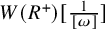 , where
$\xi \in W(R^+)$
 is a generator of the kernel of
$W(R^+)\rightarrow R^{\sharp ,+}$
 , and
$\omega \in R^+$
 is a pseudo-uniformizer. Note that

if
$R^{\sharp }$
 is of characteristic
$0$
 , and

if
$S^{\sharp }=S$
 , where
$\mathbb {B}_{\mathrm {dR}}^+(R^{\sharp }) $
 is the
$\xi $
 -adic completion of
$W(R^+)[\frac {1}{p}]$
 with
$\xi \in W(R^+)$
 being a generator of the kernel of the canonical map
$W(R^{+})[\frac {1}{p}] \rightarrow R^{\sharp }$
 .
When we have finitely many untilts
$S_i^{\sharp } = \mathrm {Spa}(R^{\sharp }_i,R^{\sharp ,+}_i)$
 of S (possibly not all distinct), we denote

where
$\xi = \prod \xi _i$
 with
$\xi _i$
 a generator of the kernel of
$W(R^+)\rightarrow R_i^{\sharp ,+}$
 .
We will frequently use the formal properties of cohomological correspondences. Let
$X,Y$
 and Z be small v-stacks that form a diagram

where we assume that t is compactifiable, representable in locally spatial diamonds with locally dim.trg
$< \infty $
 . Let
$\Lambda = \mathcal {O}_K$
 with K a finite extension of
$\mathbb {Q}_\ell $
 ,
$A\in D_{\text {\'{e}t}}(X,\Lambda )$
 and
$B \in D_{\text {\'{e}t}}(Y,\Lambda )$
 . Then a cohomological correspondence from A to B supported on Z, denoted by

is defined to be a morphism

in
$D_{\text {\'{e}t}}(Z,\Lambda )$
 .
Let us be given a commutative diagram

of small v-stacks. Let
$\mathscr {C} : (X,A) \rightarrow (Y,B)$
 be a cohomological correspondence supported on Z. Then we can pull back
$\mathscr {C}$
 along the diagram to obtain a cohomological correspondence

supported on
$\mathcal {Z}$
 , if either the right square of the diagram is Cartesian or
$f,g$
 and h are cohomologically smooth, see [Reference Xiao and ZhuXZ17, Appendix A.2.11].
On the other hand, let
$\mathscr {C} : (\mathcal {X},A) \rightarrow (\mathcal {Y},B)$
 be a cohomological correspondence supported on
$\mathcal {Z}$
 , and suppose that
$s'$
 and s are proper. Then we can !-pushforward
$\mathscr {C}$
 to obtain a cohomological correspondence

supported on Z, see [Reference Xiao and ZhuXZ17, Appendix A.2.6].
Moreover, we can compose cohomological correspondences, and pullback and !-pushforward commute with composition, see appendix A.2 of
$loc.cit$
 . The cohomological correspondences and their relation with 6-functor formalism are studied systematically in more recent works, see [Reference Heyer and MannHM24] and [Reference Lu and ZhengLZ22].
2 Basic definitions
Let G be a reductive group over
$\mathbb {Q}_p$
 , together with a reductive model
$\mathcal {G}$
 over
$\mathbb {Z}_p$
 . Then G is unramified, so split over
 , where
 . Let
$\mu $
 be a conjugacy class of cocharacters
$\mathbb {G}_m \rightarrow G_{\overline {\mathbb {Q}_p}}$
 , whose field of definition is E, which is contained in
 (by the unramifiedness of G).
Let us first introduce the notation that we will use frequently. Let S be an affinoid perfectoid space of characteristic p,
$\mathcal {P}_1$
 and
$ \mathcal {P}_{2}\, \mathcal {G}$
 -torsors on
$\mathcal {Y}_{[0,\infty )}(S)$
 , and
$S^{\sharp }$
 an untilt of S. We will use the dotted arrow

to denote a modification from
$\mathcal {P}_1$
 to
$\mathcal {P}_2$
 , that is,
$\varphi $
 is an isomorphism

that is meromorphic at
$S^{\sharp }$
 , in the sense of [Reference Scholze and WeinsteinSW20, Definition 5.3.5]. We can also have modifications with respect to finitely many untilts of S.
Let
$ \mu $
 be a dominant cocharacter of G. We will say that
$\varphi $
 is bounded by
$\mu $
 at
$S^{\sharp }$
 if for any geometric rank 1 point C of S, and trivializations of
$\mathcal {P}_1$
 and
$\mathcal {P}_2$
 over
$\mathcal {O}^{\land }_{\mathcal {Y}_{[0,\infty )}(C), C^{\sharp }} [\frac {1}{\xi }]$
 , the “punctured formal neighborhood of
$C^{\sharp }$
 ,”
$\varphi $
 lies in
$\mathcal {G}(\mathcal {O}^{\land }_{\mathcal {Y}_{[0,\infty )}(C), C^{\sharp }}) \lambda (\xi ) \mathcal {G}(\mathcal {O}^{\land }_{\mathcal {Y}_{[0,\infty )}(C), C^{\sharp }})$
 for some
$\lambda \leq \mu $
 , where
$\xi \in \mathcal {O}^{\land }_{\mathcal {Y}_{[0,\infty )}(C), C^{\sharp }}$
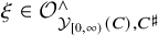 is a uniformizer, and
$\lambda (\xi ) \in G(\mathcal {O}^{\land }_{\mathcal {Y}_{[0,\infty )}(C), C^{\sharp }} [\frac {1}{\xi }])$
 is the image of
$\xi $
 under (
$\mathcal {O}^{\land }_{\mathcal {Y}_{[0,\infty )}(C), C^{\sharp }} [\frac {1}{\xi }]$
 -points of)
$\lambda $
 . Note that this is a pointwise condition on S.
The definitions introduced below are only prestacks a priori, but it follows directly from [Reference Scholze and WeinsteinSW20, Proposition 19.5.3] and [Reference Scholze and WeinsteinSW20, Corollary 17.1.9] that they are all stacks, with the exception of (global) Witt vector shtukas and Hecke stacks in Section 2.3, where the stackification is necessary.
2.1 Hecke stacks
We first introduce Hecke stacks.
Definition 2.1. Let I be a finite set, and
$\mu _{\bullet }$
 be a collection of dominant cocharacters of G indexed by I. Let
$\{I_1, \ldots , I_k\}$
 be a partition of I. We define

to be the stack over  (
 ) whose value at S is the groupoid of
$\bullet \, \mathcal {G}$
 -torsors
$\mathcal {P}_1, \ldots , \mathcal {P}_{k+1}$
 on
$\mathcal {Y}_{[0,\infty )}(S)$

$\bullet $
 untilts
$S^{\sharp }_i \hookrightarrow \mathcal {Y}_{[0,\infty )}(S)$
 of S defined over
 indexed by
$i\in I$
 , and
$\bullet $
 modifications

where the dotted arrows
$\varphi _i$
 are isomorphisms

that are meromorphic along the Cartier divisor
$ \underset {j \in I_i}{\sum } S^{\sharp }_j $
 of
$ \mathcal {Y}_{[0,\infty )}(S)$
 .
We define

to be the closed substack of
$\mathrm {Hecke}_{}^{(I_1, \ldots , I_k)}$
 parametrizing the data as
$\mathrm {Hecke}_{}^{(I_1, \ldots , I_k)}$
 does with the additional condition that at every geometric rank 1 point C of S and untilt
$C^{\sharp }$
 of C,
$\varphi _i$
 is bounded by
$\underset { \begin {subarray}{c} j \in I_i \\ C^{\sharp } \in S^{\sharp }_j \end {subarray} }{\sum } \mu _j$
 at
$C^{\sharp }$
 , where
$C^{\sharp } \in S^{\sharp }_j $
 means that the canonical untilt (over
$S_j^{\sharp }$
 ) of C over S, under the equivalence between perfectoid spaces over
$S^{\sharp }_j$
 and perfectoid spaces over S, is identified with
$C^{\sharp }$
 .
When the partition is trivial, we make the following simplification

which parametrizes

that is meromorphic and bounded by
$\mu _i$
 at each untilt
$S_i^{\sharp }$
 of S.
Remark 2.2. We note that
$\mathrm {Hecke}^{(I_1,\ldots ,I_k)}_{\mu _{\bullet }}$
 is really defined over the product of the rings of integers of the defining fields of
$\mu _{\bullet }$
 . The base can be further refined if we do not specify the boundedness condition. Indeed,
$\mathrm {Hecke}^{(I_1,\ldots ,I_k)}$
 can be naturally defined over
$\mathrm {Spd}(\mathbb {Z}_p)^I$
 , that is, it is the base change to
 of a v-stack defined over
$\mathrm {Spd}(\mathbb {Z}_p)^I$
 .
We observe that there are natural maps between Hecke stacks.
Let
$\zeta : I \rightarrow J$
 be a map of finite sets,
$(J_1, \ldots , J_k)$
 be a partition of J, and
$I_i = \zeta ^{-1}J_i$
 . There exists a natural map

where we abuse notation by writing  the permutation map corresponding to
$\zeta $
 , that is, sending
$(x_j)_{j\in J}$
 to
$(x_{\zeta (i)})_{i\in I}$
 . It is defined by sending

to itself, except we just relabel the legs using
$\zeta $
 . More precisely, it sends

to

which is the restriction of
$\varphi _i$
 to
$\mathcal {Y}_{[0,\infty )}(S)\setminus \underset {j \in J_i}{\cup } S^{\sharp }_{j}$
 , that is, the modification at
$S^{\sharp }_{j}$
 is given by
$\varphi _i$
 if
$j \in \zeta (I_i)$
 , and it is trivial if
$j \notin \zeta (I_i)$
 .
Moreover, we have the convolution map

which is defined by sending

to

Lastly, we have the maps that split the partition. Let
$(J_1, \ldots , J_l)$
 be a partition of I such that
$J_j = I_{i_j} \cup \ldots \cup I_{i_{j+1}-1}$
 for some partition
$1=i_1 < i_2 < \ldots < i_{l+1}= k+1$
 of
$k+1$
 . We define

to be the forgetful map that sends

to

Now we introduce the correspondence version for Hecke stacks.
Definition 2.3. Let
$I, J$
 be finite sets, and
$\mu _{\bullet }, \mu ^{\prime }_{\bullet }$
 be collections of dominant cocharacters of G indexed by I and J respectively. Let
$\nu $
 be a dominant cocharacter of G. Then we define

to be the stack with value at a characteristic p perfectoid space S being the groupoid of the data of
$\bullet \, \{\mathcal {P}_1, \mathcal {P}_2, \varphi \}\in \mathrm {Hecke}_{\mu _{\bullet } }(S)$
 and
$\{\mathcal {P}^{\prime }_1, \mathcal {P}_2',\varphi '\} \in \mathrm {Hecke}_{\mu ^{\prime }_{\bullet } }(S)$
 ,
$\bullet $
 (meromorphic) modifications bounded by
$\nu $


at the characteristic p untilt
$S \hookrightarrow \mathcal {Y}_{[0,\infty )}(S)$
 such that the following diagram is commutative

We will occasionally use the following more general version.
Definition 2.4. Let
$I, J$
 be finite sets, and
$\mu _{\bullet }, \mu ^{\prime }_{\bullet }$
 be collections of dominant cocharacters of G indexed by I and J respectively. Let
$\{I_1, \ldots , I_k\}$
 and
$\{J_1, \ldots , J_l\}$
 be partitions of I and J. Let
$\nu $
 be a dominant cocharacter of G. Then we define

to be the stack with value at a characteristic p perfectoid space S being the groupoid of the data of
$\bullet \, \{\mathcal {P}_1,\ldots , \mathcal {P}_{k+1}, \varphi _1, \ldots \varphi _k \}\in \mathrm {Hecke}_{\mu _{\bullet } }^{(I_1, \ldots , I_k)}(S)$
 and
$\{\mathcal {P}^{\prime }_1, \ldots , \mathcal {P}_{l+1}',\varphi ',\ldots \varphi _l'\} \in \mathrm {Hecke}_{\mu ^{\prime }_{\bullet } }^{(J_1, \ldots , J_l)}(S)$
 ,
$\bullet $
 modifications bounded by
$\nu $
 (in the sense similar to the above)


at the characteristic p untilt
$S \hookrightarrow \mathcal {Y}_{[0,\infty )}(S)$
 such that the following diagram is commutative

We will also make use of a local version of Hecke stacks, which parametrizes modifications of torsors over the formal neighborhoods of Cartier divisors corresponding to untilts.
Definition 2.5. Let I be a finite set, and
$\mu _{\bullet }$
 be a collection of dominant cocharacters of G indexed by I. Let
$\{I_1, \ldots , I_k\}$
 be a partition of I. We define

to be the stack over  whose value at S is the groupoid of
$\bullet $
 untilts
$S^{\sharp }_i$
 of S defined over
 indexed by
$i\in I$
 ,
$\bullet \, \mathcal {G}$
 -torsors
$\mathcal {P}_1, \ldots , \mathcal {P}_{k+1}$
 on
$Spec(\mathcal {O}^{\land }_{\mathcal {Y}_{[0,\infty )}(S), \sum S_i^{\sharp }})$
 , and,
$\bullet $
 modifications

where the dotted arrows
$\varphi _i$
 are isomorphisms

such that at every geometric rank 1 point C of S and untilt
$C^{\sharp }$
 of C,
$\varphi _i$
 is bounded by
$\underset { \begin {subarray}{c} j \in I_i \\ C^{\sharp } \in S^{\sharp }_j \end {subarray} }{\sum } \mu _j$
 at
$C^{\sharp }$
 .
When the partition is trivial, we make the following simplification

Lastly, we denote

Remark 2.6. When the partition of I is trivial, the local Hecke stack is defined in [Reference Fargues and ScholzeFS21, Definition VI.1.6]. The general partition case also appears in the proof of [Reference Fargues and ScholzeFS21, Definition/proposition VI.9.4].
Remark 2.7. The drawback of local Hecke stacks is that there is no obvious correspondence between them, due to that the torsors are defined on different domains. However, this problem disappears if we fix the legs at characteristic p untilts. An important example is the Witt vector local Hecke stacks to be defined below, where we have the correspondences.
There is a canonical map

being the restriction from global G-torsors to local G-torsors. We will use it to define the Satake sheaves on
$\mathrm {Hecke}_{\mu _{\bullet }}^{(I_1, \ldots , I_k)}$
 .
Let
$L^{+}\mathcal {G} $
 be the group v-sheaf over
 whose value at S is

and  the Beilinson–Drinfeld affine Grassmannian as defined in [Reference Scholze and WeinsteinSW20, Definition 20.3.1], which classifies
$\mathcal {G}$
 -torsors on the formal neighborhood of
$S^{\sharp }$
 together with a trivialization of the generic fiber that is bounded by
$\mu $
 . By [Reference Scholze and WeinsteinSW20, Proposition 20.5.4],
 is representable in spatial diamonds, and so is in particular a small v-sheaf. By definition, we have

as a stack quotient, where
$L^{+}\mathcal {G}$
 acts on the trivialization, so
$\mathrm {Hecke}_{\mu }^{{\mathrm {loc}}}$
 is a small v-stack.
We have a similar expression for the global Hecke stack
$\mathrm {Hecke}_{\mu }$
 , which can be written as the quotient of
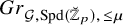 by the group v-sheaf parametrizing automorphisms of the trivial global
$\mathcal {G}$
 -torsor on
$\mathcal {Y}_{[0,\infty )}$
 . Moreover, for Hecke stacks with multiple legs, they can be written again as quotients of twisted products of affine Grassmannians, see the beginning of [Reference Fargues and ScholzeFS21, Chapter VI] (for the version of local Hecke stacks).
If the characteristic of the untilt
$S^{\sharp }$
 is p, then
$S^{\sharp } = S$
 , and

if
$S=\mathrm {Spa}(R,R^{+})$
 . Then the fiber of the Beilinson–Drinfeld affine Grassmannian at the characteristic p untilt is the Witt vector affine Grassmannian considered in [Reference ZhuZhu17].Footnote
1
On the other hand, if
$S^{\sharp }=\mathrm {Spa}(R^{\sharp },R^{\sharp ,+})$
 is a characteristic zero untilt, we have

and the fiber of  at
$S^{\sharp }$
 is the
$\mathbb {B}^+_{\text {dR}}$
 -affine Grassmannian as defined in [Reference Scholze and WeinsteinSW20, Lecture 19].
Similar to global Hecke stacks, there are natural maps between local Hecke stacks.
Let
$\zeta : I \rightarrow J$
 be a map of finite sets,
$(J_1, \ldots , J_k)$
 be a partition of J, and
$I_i = \zeta ^{-1}J_i$
 . There exists a natural map

where we abuse notation by writing  the permutation map corresponding to
$\zeta $
 , that is, sending
$(x_j)_{j\in J}$
 to
$(x_{\zeta (i)})_{i\in I}$
 . It is defined by sending

to itself, except we just relabel the legs using
$\zeta $
 . More precisely, it sends

to

where the modification at
$S^{\sharp }_{j}$
 is given by
$\varphi _i$
 if
$j \in \zeta (I_i)$
 , and it is trivial, that is, no modification at all, if
$j \notin \zeta (I_i)$
 .
Moreover, we have the convolution map

which is defined by sending

to

Lastly, we have the maps that split the partition. Let
$(J_1, \ldots , J_l)$
 be a partition of I such that
$J_j = I_{i_j} \cup \ldots \cup I_{i_{j+1}-1}$
 for some partition
$1=i_1 < i_2 < \ldots < i_{l+1}= k+1$
 of
$k+1$
 . We define

to be the forgetful map that sends

to

Notation 2.8. Throughout the paper, we use the following notation to denote the restriction to the generic fiber,


Similarly for the restriction to the special fiber,


We also have the mixed version, for example

2.2 Moduli spaces of p-adic shtukas
We now introduce the critical objects of study in this article, the moduli spaces of shtukas.
Definition 2.9. The moduli space of shtukas associated to
$\mathcal {G}$
 and
$\mu $
 is the stack

over  whose value at a characteristic p perfectoid space S is the groupoid of the data of
$\bullet $
 a
$\mathcal {G}$
 -torsor
$\mathcal {P}$
 over
$\mathcal {Y}_{[0,\infty )}(S)$
 ,
$\bullet $
 an (not necessarily of characteristic 0) untilt
$S^{\sharp } \hookrightarrow \mathcal {Y}_{[0,\infty )}(S)$
 of S defined over
 , and
$\bullet $
 an isomorphism

that is meromorphic along the Cartier divisor
$S^{\sharp } \hookrightarrow \mathcal {Y}_{[0,\infty )}(S)$
 , and bounded by
$\mu $
 .
Remark 2.10. Although we work with the base  , the definition of moduli spaces of shtukas really depends on the group
$\mathcal {G}$
 over
$\mathbb {Z}_p$
 rather than its base change to
 , as otherwise the Frobenius pullback
$\mathrm {Frob}_S^*\mathcal {P}$
 does not make sense (it would be a torsor with respect to a Frobenius twist of the structure group over
 ).
Remark 2.11. The definition given here is close to the classical function field counterpart, which is slightly different from the ones in [Reference Scholze and WeinsteinSW20, Definition 25.1.1 and 23.3.1] in that we do not fix a trivialization of the
$\mathcal {G}(\mathbb {Z}_p)$
 -torsor as in
$loc.cit.$
 , nor do we fix the type of shtukas in
$B(G)$
 . The treatment in
$loc.cit.$
 is to emphasize the way moduli spaces of shtukas generalize Rapoport–Zink spacesFootnote
2
, whereas we want to mimic the treatment of Lafforgue in [Reference LafforgueLaf18].
We will also make use of moduli spaces of shtukas with several legs.
Definition 2.12. Let I be a finite set, and
$\mu _{\bullet }$
 be a collection of dominant cocharacters of G indexed by I. Let
$\{I_1, \ldots , I_k\}$
 be a partition of I. The moduli space of shtukas associated to G,
$\mu _{\bullet }$
 , and
$\{I_1, \ldots , I_k\}$
 is the stack

over  whose value at a characteristic p perfectoid space S is the groupoid of the data of
$\bullet \, \mathcal {G}$
 -torsors
$\mathcal {P}_1, \ldots , \mathcal {P}_k$
 over
$\mathcal {Y}_{[0,\infty )}(S)$
 ,
$\bullet $
 (not necessarily of characteristic 0) untilts
$S^{\sharp }_i \hookrightarrow \mathcal {Y}_{[0,\infty )}(S)$
 of S defined over
 indexed by
$i\in I$
 , and
$\bullet $
 modifications

where the dotted arrows
$\varphi _i$
 are isomorphisms

with
$\mathcal {P}_{k+1} =\mathrm {Frob}_S^*\mathcal {P}_1$
 , which are meromorphic along the Cartier divisor
$ \underset {j \in I_i}{\sum } S^{\sharp }_j $
 of
$ \mathcal {Y}_{[0,\infty )}(S)$
 . Moreover, at every geometric rank 1 point C of S and untilt
$C^{\sharp }$
 of C,
$\varphi _i$
 is bounded by
$\underset { \begin {subarray}{c} j \in I_i \\ C^{\sharp } \in S^{\sharp }_j \end {subarray} }{\sum } \mu _j$
 at
$C^{\sharp }$
 .
When the partition is trivial, we drop the superscript to simplify the notation, that is,

which parametrizes isomorphisms of
$\mathcal {G}$
 -torsors

that is meromorphic and bounded by
$\mu _i$
 at each untilt
$S_i^{\sharp }$
 of S.
The following variant defines a correspondence between moduli spaces of shtukas and will be very important for our purposes.
Definition 2.13. Let
$\mu , \mu ' $
 and
$\nu $
 be conjugacy classes of cocharacters
$\mathbb {G}_m \rightarrow G_{\overline {\mathbb {Q}_p}}$
 . We define

to be the stack over  with value at a characteristic p perfectoid space S being the groupoid of the data of
$\bullet \, \mathcal {P} \in \mathrm {Sht}_{\mu }(S)$
 and
$\mathcal {P}' \in \mathrm {Sht}_{\mu '}(S)$
 ,
$\bullet $
 a meromorphic modification

at the characteristic p untilt
$S \hookrightarrow \mathcal {Y}_{[0,\infty )}(S)$
 as shtukas, that is, the following diagram is commutative

with the notation that dashed arrows denote generically defined modifications.
We define

to be the closed substack of
$\mathrm {Sht}_{\mu |\mu '}$
 parametrizing the data as
$\mathrm {Sht}_{\mu |\mu '}$
 does with the additional condition that
$\gamma $
 is bounded by
$\nu $
 .
Similarly, we have the version for moduli spaces of shtukas with several legs.
Definition 2.14. Let
$I, J$
 be finite sets, and
$\mu _{\bullet }, \mu ^{\prime }_{\bullet }$
 be collections of dominant cocharacters of G indexed by I and J respectively. Let
$\{I_1, \ldots , I_k\}$
 and
$\{J_1, \ldots , J_l\}$
 be partitions of I and J. Let
$\nu $
 be a dominant cocharacter of G. Then we define

to be the stack with value at a characteristic p perfectoid space S being the groupoid of the data of
$\bullet \, \{\mathcal {P}_1, \ldots , \mathcal {P}_k, \varphi _1,\ldots , \varphi _k \} \in \mathrm {Sht}^{(I_1, \ldots , I_k)}_{\mu _{\bullet } }(S)$
 and
$\{\mathcal {P}_1', \ldots , \mathcal {P}_l', \varphi _1', \ldots , \varphi _l'\} \in \mathrm {Sht}^{(J_1, \ldots , J_l)}_{\mu ^{\prime }_{\bullet } }(S)$
 ,
$\bullet $
 a modification bounded by
$\nu $
 (in the sense similar to the above)

at the characteristic p untilt
$S \hookrightarrow \mathcal {Y}_{[0,\infty )}(S)$
 as shtukas, that is, the following diagram is commutative

When the partitions of I and J are trivial, we will simplify the notation by writing

which parametrizes commutative diagrams

where
$\varphi _{\mathcal {P}}$
 (resp.
$\varphi _{\mathcal {P}'}$
 ) is meromorphic and bounded by
$\sum _i \mu _i$
 (resp.
$\sum _{j}\mu _j'$
 ) at each untilt
$S^{\sharp }$
 of S, where
$i $
 (resp. j) ranges over
$i\in I$
 (resp.
$j\in J$
 ) for which
$S_i^{\sharp } = S^{\sharp }$
 (resp.
$S_j^{\sharp } = S^{\sharp }$
 ).
Remark 2.15. Let
$E_i$
 be the reflex field of
$\mu _i$
 . Then
$\mathrm {Sht}_{\mu _{\bullet }}^{(I_1,\ldots ,I_k)}$
 is actually defined over
$\prod \mathrm {Spd}(\mathcal {O}_{E_i})$
 , and similarly for
$\mathrm {Sht}^{(I_1, \ldots , I_k)|(J_1, \ldots , J_l), \nu }_{\mu _{\bullet }|\mu _{\bullet }'}$
 . The same refinement works for all the spaces defined in this section.
Notation 2.16. We will use notation similar to that in Notation 2.8 for the restriction of moduli spaces of shtukas to the generic fiber,


and in particular

Note that in the last case,
$\mu $
 has to be equal to
$\mu '$
 .
Similarly, we have the restriction to the special fiber


We also have the mixed version, for example

We have the following alternative characterization of moduli spaces of shtukas over the generic fiber.
Theorem 2.17.
$\mathrm {Sht}_{\mu , \eta }$
 is equivalent to the stack over
 sending a characteristic p perfectoid space S over
 to the groupoid of
$\bullet \, G$
 -torsors
$\mathcal {E}_0$
 and
$\mathcal {E}$
 over the Fargues–Fontaine curve
$\mathcal {X}_{\mathrm {FF}, S}$
 such that
$\mathcal {E}_0$
 is trivial at every geometric point of S. The data
$\mathcal {E}_0$
 is equivalent to a pro-étale
$G(\mathbb {Q}_p)$
 -torsor
$\mathbb {L}_{\eta }$
 on S by [Reference Kedlaya and LiuKL15, Theorem 8.5.5],
$\bullet $
 an untilt
$S^{\sharp } \hookrightarrow \mathcal {Y}_{[0,\infty )}(S)$
 of S defined over
 ,
$\bullet $
 an isomorphism

that is meromorphic along
$S^{\sharp }$
 and bounded by
$\mu $
 ,
$\bullet $
 a sub-
$\mathcal {G}(\mathbb {Z}_p)$
 -torsor
$\mathbb {L}$
 inside
$\mathbb {L}_{\eta }$
 .
Proof. The proof of [Reference Scholze and WeinsteinSW20, Proposition 23.3.1] goes without change. Indeed, in
$loc. cit.$
 they fix the type of shtukas in
$\mathrm {B}(G)$
 , which corresponds to rigidifying
$\mathcal {E}$
 . Dropping this extra condition gives exactly the data as in the statement.
We have a natural correspondence diagram

where
$p_1$
 (resp.
$p_2$
 ) sends
$\{\mathcal {P}, \mathcal {P}', \gamma ,S^{\sharp }\}$
 to
$\{\mathcal {P},S^{\sharp }\}$
 (resp.
$\{\mathcal {P}',S^{\sharp }\}$
 ).
Proposition 2.18. The correspondence (7) is an étale correspondence, that is, both
$p_1$
 and
$p_2$
 are finite étale morphisms.
Proof. With the characterization of Theorem 2.17, we see that
$\mathrm {Sht}_{\mu |\mu ,\eta }^{\nu }(S)$
 parametrizes
$\bullet \, \{ \mathcal {E}_0, \mathcal {E}, \alpha , \mathbb {L}, S^{\sharp } \} \in \mathrm {Sht}_{\mu ,\eta }(S)$
 ,
$\bullet \, \{ \mathcal {E}^{\prime }_0, \mathcal {E}', \alpha ', \mathbb {L}', S^{\sharp } \} \in \mathrm {Sht}_{\mu ,\eta }(S)$
 ,
$\bullet $
 isomorphisms


such that
$\alpha ' \circ \beta _0 = \beta \circ \alpha $
 , and under the isomorphism

of pro-étale
$G(\mathbb {Q}_p)$
 -torsors on S induced by
$\beta _0$
 , the sub-
$\mathcal {G}(\mathbb {Z}_p)$
 -torsors
$\mathbb {L}$
 and
$\mathbb {L}'$
 have relative position bounded by
$\nu $
 at every rank 1 geometric point of S.
Now for a given S-point of
$\mathrm {Sht}_{\mu ,\eta }$
 specified by the data
$\{ \mathcal {E}_0, \mathcal {E}, \alpha , \mathbb {L}, S^{\sharp } \} \in \mathrm {Sht}_{\mu ,\eta }(S)$
 , we see that the fiber of
$p_1$
 at this point is the data of sub-
$\mathcal {G}(\mathbb {Z}_p)$
 -torsors
$\mathbb {L}'$
 of
$\mathbb {L}_{\eta }$
 which have relative position with respect to
$\mathbb {L}$
 bounded by
$\nu $
 at every geometric point of S. Since pro-étale locally
$\mathbb {L}_{\eta }$
 is the trivial torsor
$S \times G(\mathbb {Q}_p)$
 , the relevant sub-
$\mathcal {G}(\mathbb {Z}_p)$
 -torsors correspond to a finite subset of
$G(\mathbb {Q}_p)/\mathcal {G}(\mathbb {Z}_p)$
 determined by
$\nu $
 Footnote
3
, which is visibly finite étale over S. Thus we see that
$p_1$
 is finite étale after base change to a pro-étale cover; hence, it is finite étale by [Reference ScholzeSch17, Corollary 9.11 (iii)].
The same argument shows that
$p_2$
 is finite étale.
2.3 Moduli spaces of Witt vector shtukas and Witt vector Hecke stacks
We will need the Witt vector version of moduli spaces of shtukas and Hecke stacks as well.
Definition 2.19. Let I be a finite set, and
$\mu _{\bullet }$
 be a collection of dominant cocharacters of G indexed by I. The moduli space of Witt vector shtukas over
$ \mathrm {Spd}(\overline {\mathbb {F}_p})$
 associated to G and
$\mu _{\bullet }$
 , denoted by

is the stackification of the prestack sending a characteristic p affinoid perfectoid space
$S=Spa(R,R^+)$
 over
$\overline {\mathbb {F}_p}$
 to the groupoid of the data of
$\bullet \, \mathcal {G}$
 -torsors
$\mathcal {P}_1, \ldots , \mathcal {P}_k$
 over
$\mathrm {Spec}(W(R^+))$
 , and
$\bullet $
 modifications

where the dotted arrows
$\varphi _i$
 are isomorphisms

with
$\mathcal {P}_{k+1} =\mathrm {Frob}_S^*\mathcal {P}_1$
 , which are bounded by
$\mu _i$
 at every geometric point of S.
We have the local version as well, which is already a stack by [Reference Scholze and WeinsteinSW20, Corollary 17.1.9].
Definition 2.20. Let I be a finite set, and
$\mu _{\bullet }$
 be a collection of dominant cocharacters of G indexed by I. The moduli space of Witt vector local shtukas associated to G and
$\mu _{\bullet }$
 is the stack

over
$ \mathrm {Spd}(\overline {\mathbb {F}_p})$
 whose value at a characteristic p affinoid perfectoid space S over
$\overline {\mathbb {F}_p}$
 is the groupoid of the data of
$\bullet \, \mathcal {G}$
 -torsors
$\mathcal {P}_1, \ldots , \mathcal {P}_k$
 over
$\mathrm {Spec}(\mathcal {O}^{\wedge }_{\mathcal {Y}_{[0,\infty )}(S), S} )$
 , and
$\bullet $
 modifications

where the dotted arrows
$\varphi _i$
 are isomorphisms

with
$\mathcal {P}_{k+1} =\mathrm {Frob}_S^*\mathcal {P}_1$
 , which are bounded by
$\mu _i$
 at every geometric point of S.
The possibility of having such a definition comes from the fact that Frobenius fixes the characteristic p legs, which is not the case for the characteristic 0 ones.
Remark 2.21. Note that there is no extra data on the partition of I since we fix legs at the characteristic p untilt, so essentially the only possibility of the partition is
$(\{1\}, \ldots , \{k\})$
 . For example, moduli spaces of Witt vector shtukas with respect to
$(\{1,2 \}, \{3\} )$
 and cocharacters
$\{\mu _1, \mu _2, \mu _3\}$
 are the same as moduli spaces of Witt vector shtukas with respect to
$(\{1 \}, \{2\} )$
 and cocharacters
$\{\mu _1 +\mu _2, \mu _3\}$
 .
Again, there is the correspondence version.
Definition 2.22. Let
$I, J$
 be finite sets, and
$\mu _{\bullet }, \mu ^{\prime }_{\bullet }$
 be collections of dominant cocharacters of G indexed by I and J respectively. Let
$\nu $
 be a dominant cocharacter of G. Then we define

to be the stackification of the prestack sending a characteristic p affinoid perfectoid space
$S=Spa(R,R^+)$
 over
$\overline {\mathbb {F}_p}$
 to the groupoid of the data of
$\bullet \, \{\mathcal {P}_1, \ldots , \mathcal {P}_k, \varphi _1,\ldots , \varphi _k \} \in \mathrm {Sht}^{W}_{\mu _{\bullet } }(S)$
 and
$\{\mathcal {P}_1', \ldots , \mathcal {P}_l', \varphi _1', \ldots , \varphi _l'\} \in \mathrm {Sht}^{W}_{\mu ^{\prime }_{\bullet } }(S)$
 ,
$\bullet $
 a modification bounded by
$\nu $


as shtukas, that is, the following diagram is commutative

We now define the Witt vector Hecke stacks.
Definition 2.23. Let I be a finite set, and
$\mu _{\bullet }$
 be a collection of dominant cocharacters of G indexed by I. We define

to be the stackification of the prestack sending
$S=Spa(R,R^+)$
 over
$\overline {\mathbb {F}_p}$
 to the groupoid of
$\bullet \, \mathcal {G}$
 -torsors
$\mathcal {P}_1, \ldots , \mathcal {P}_{k+1}$
 on
$Spec(W(R^+))$
 ,
$\bullet $
 modifications

where the dotted arrows
$\varphi _i$
 are isomorphisms

that are bounded by
$\mu _i$
 at every geometric point of S.
Remark 2.24. One can also define a local version of the Witt vector Hecke stack, but this coincides with the special fiber of
$\mathrm {Hecke}^{\mathrm {loc}}_{\mu _{\bullet }}$
 .
Definition 2.25. Let
$I, J$
 be finite sets, and
$\mu _{\bullet }, \mu ^{\prime }_{\bullet }$
 be collections of dominant cocharacters of G indexed by I and J respectively. Let
$\nu $
 be a dominant cocharacter of G. Then we define

to be the stackification of the prestack sending a characteristic p affinoid perfectoid space
$S=Spa(R,R^+)$
 over
$\overline {\mathbb {F}_p}$
 to the groupoid of the data of
$\bullet \, \{\mathcal {P}_1,\ldots , \mathcal {P}_{k+1}, \varphi _1, \ldots \varphi _k \}\in \mathrm {Hecke}_{\mu _{\bullet } }^{W}(S)$
 and
$\{\mathcal {P}^{\prime }_1, \ldots , \mathcal {P}_{l+1}',\varphi ',\ldots \varphi _l'\} \in \mathrm {Hecke}_{\mu ^{\prime }_{\bullet } }^{W}(S)$
 ,
$\bullet $
 modifications bounded by
$\nu $


such that the following diagram is commutative

We observe that the moduli spaces of Witt vector shtukas and Hecke stacks are analytifications of perfect stacks. Let
$\mathrm {Hecke}^{\mathrm {loc}(\infty )}_{\mu _{\bullet }}$
 be the perfect Hecke stack as defined in [Reference Xiao and ZhuXZ17, Definition 5.1.1]; see also Appendix A.3. Then it is easy to see that

and

with notations as in A.1. On the other hand, we have

and

where
$\mathrm {Sht}_{\mu _{\bullet }}^{\mathrm {loc}(\infty )}$
 is the untruncated moduli space of Witt vector shtukas defined in [Reference Xiao and ZhuXZ17, Definition 5.2.1]. Similarly for the correspondence version
$\mathrm {Hecke}^{\nu ,W}_{\mu _{\bullet }|\mu _{\bullet }'}$
 and
$ \mathrm {Sht}^{\nu ,W}_{\mu _{\bullet }|\mu _{\bullet }'}$
 .
As a sanity check, all the stacks defined above are small v-stacks.
Proposition 2.26.
$\mathrm {Hecke}_{\mu _{\bullet }}^{(I_1,\ldots ,I_k)}$
 ,
$\mathrm {Hecke}_{\mu _{\bullet }}^{\mathrm {loc},(I_1,\ldots ,I_k)}$
 ,
$ \mathrm {Hecke}^{(I_1, \ldots , I_k)|(J_1, \ldots , J_l), \nu }_{\mu _{\bullet }|\mu _{\bullet }'}$
 ,
$\mathrm {Hecke}^W_{\mu _{\bullet }}$
 ,
$\mathrm {Hecke}^{\nu ,W}_{\mu _{\bullet }|\mu _{\bullet }'}$
 ,
$\mathrm {Sht}_{\mu _{\bullet }}^{(I_1,\ldots ,I_k)}$
 ,
$\mathrm {Sht}_{\mu _{\bullet }}^{\mathrm {loc},W}$
 ,
$\mathrm {Sht}_{\mu _{\bullet }}^W$
 ,
$\mathrm {Sht}^{\nu ,W}_{\mu _{\bullet }|\mu _{\bullet }'}$
 and
$\mathrm {Sht}^{(I_1, \ldots , I_k)|(J_1, \ldots , J_l),\nu }_{\mu _{\bullet }|\mu ^{\prime }_{\bullet }} $
 are small v-stacks.
Proof. See the proof of [Reference Fargues and ScholzeFS21, Proposition III.1.3].
3 The geometric Satake
We follow the same notation as in the previous section. Moreover, we define the derived category of a small v-stack X with
$\overline {\mathbb {Q}}_\ell $
 -coefficient to be

where E ranges over subfields of
$\overline {\mathbb {Q}}_\ell $
 that are finite extensions of
$\mathbb {Q}_\ell $
 ,
$D^b_{\text {\'{e}t}}(X,E) $
 is the idempotent completion of
$D^b_{\text {\'{e}t}}(X,\mathcal {O}_E) [\frac {1}{l}]$
 and the colimit is taken in the
$\infty $
 -categorical sense. Recall that the derived category
$D^b_{\text {\'{e}t}}(X,\mathcal {O}_E)$
 with adic coefficients is defined in [Reference ScholzeSch17, Section 26]. The six-functor formalism generalizes directly to this setting.
Remark 3.1. The constructions in this paper already work with the coefficient ring
$\mathcal {O}_{\mathbb {Q}_\ell (\sqrt {q})}$
 , and we can work with that instead.
Remark 3.2. The definition given here compares favorably with the constructible derived categories of schemesFootnote 4 , see [Reference Bhatt and ScholzeBS15, Section 6.8] or [Reference Hemo, Richarz and ScholbachHRS23], which suffices for our purposes in this paper. Moreover, the comparison functor from schemes to the associated diamonds is fully faithful, see [Reference ScholzeSch17, Proposition 27.2] and the appendix.
Let us recall the geometric Satake proved by Fargues–Scholze.
Theorem 3.3. (Fargues–Scholze)
Let
$I $
 be a finite set, and
$\mu _{\bullet }$
 be a collection of dominant geometric cocharacters of G indexed by I. Let
$\{I_1, \ldots , I_k\}$
 be a partition of I. There is a natural functor

from the category of representations of
$\hat {G}^I$
 , the product of the dual group of G (with
$\overline {\mathbb {Q}}_\ell $
 -coefficient), to the category
$D_{\text {\'{e}t}}^b(\mathrm {Hecke}^{\mathrm {loc},(I_1, \ldots , I_k)}, \overline {\mathbb {Q}}_\ell )$
 . It has the following properties.
1) If U is irreducible with highest weight
$\mu _{\bullet }$
 , then
$\mathscr {S}_U^{\mathrm {loc},(I_1, \ldots , I_k)}$
 is supported on
$\mathrm {Hecke}_{\mu _{\bullet }}^{\mathrm {loc},(I_1, \ldots , I_k)}$
 .
2) Let
$\zeta : I \rightarrow J$
 be a map of finite sets,
$(J_1, \ldots , J_k)$
 be a partition of J, and
$I_i = \zeta ^{-1}J_i$
 . Then there exists a canonical isomorphism

where

is defined in (4),

is the projection onto the first factor, and
$\Delta _{\zeta }: \hat {G}^J \rightarrow \hat {G}^I$
 is the map sending
$(g_j)_{j\in J}$
 to
$(g_{\zeta (i)})_{i\in I}$
 .
3) There is a canonical isomorphism

where

is the convolution map defined in (5).
4) Let
$(J_1, \ldots , J_l)$
 be a partition of I such that
$J_j = I_{i_j} \cup \ldots \cup I_{i_{j+1}-1}$
 for some partition
$1=i_1 < i_2 < \ldots < i_{l+1}= k+1$
 of
$k+1$
 . Then we have a canonical isomorphism

where

is defined in (6), and
$U_j$
 is a representation of
$\hat {G}^{J_j}$
 .
5) We have a canonical isomorphism

compatible with the isomorphisms in 1), 2),3) and 4), where r is the natural restriction map

from the local Hecke stack to the truncated Witt vector Hecke stack
$X=\mathrm {Hecke}^{\mathrm {loc}(m)}_{\mu _{\bullet }}$
 as defined in [Reference Xiao and ZhuXZ17, Definition 5.1.2] and recalled in Appendix A.3, U is irreducible with highest weight
$\mu _{\bullet }$
 ,
$c_X$
 is the comparison functor defined in Appendix A.1, and
$A_{\mu _{\bullet }}$
 is the Satake sheaf on
$\mathrm {Hecke}^{\mathrm {loc}(m)}_{\mu _{\bullet }}$
 . More precisely,
$A_{\mu _{\bullet }}$
 is the descent of the intersection sheaf
$\mathrm {IC}_{\mu _{\bullet }}$
 , as defined in [Reference Xiao and ZhuXZ17, Section 3.4.1], on the Witt vector affine Grassmannian
$Gr_{\mu _{\bullet }}$
 , which exists by the
$L^+G$
 -equivariance of
$\mathrm {IC}_{\mu _{\bullet }}$
 .
Proof. It is enough to work with coefficients in the ring of integers of
$\mathbb {Q}_\ell [\sqrt {q}]$
 , which is treated in [Reference Fargues and ScholzeFS21]. We follow the ideas in the proof of [Reference LafforgueLaf18, Theorem 1.17].
Let us first consider the case that
$U=\underset {j}{\boxtimes } U_j$
 , where
$U_j$
 is a representation of
$\hat {G}^{I_j}$
 . From the geometric Satake proved in [Reference Fargues and ScholzeFS21, Theorem VI.11.1], there exists a canonical perverse sheaf
$\mathscr {S}_V^{\mathrm {loc},(J)}$
 on
$\mathrm {Hecke}^{\mathrm {loc},(J)}$
 for each representation V of
$\hat {G}^J$
 . Let
$\{ I_1, \ldots I_k\}$
 be a partition of I, and we define

Let
$\mathcal {R}_j$
 be the algebra of regular functions on
$\hat {G}^{I_j}$
 , which we view as an ind-(finite-dimensional) representation of
$\hat {G}^{I_j}$
 through the left regular representation, and we define

where the colimit is over all (finite-dimensional) subrepresentations of
$\underset {j}{\boxtimes } \mathcal {R}_j$
 that are of the form
$\underset {j}{\boxtimes } U_j$
 with
$U_j$
 representations of
$\hat {G}^{I_j}$
 .
Now let U be an arbitrary (finite-dimensional) representation of
$\hat {G}^I$
 . We define

where
$\hat {G}^{I}$
 acts diagonally on the tensor product, and
$(-)^{\hat {G}^{I}}$
 means taking
$\hat {G}^{I}$
 -invariants. The action of
$\hat {G}^{I}$
 on
$\underset {j}{\boxtimes } \mathcal {R}_j$
 is through right multiplication on
$\hat {G}^{I}$
 , so it is an action in the category of representations of
$\hat {G}^{I}$
 (recall that we view
$\mathcal {R}_j$
 as a left regular representation), which gives rise to an action of
$\hat {G}^{I}$
 on
$\mathscr {S}_{\underset {j}{\boxtimes } \mathcal {R}_j}^{\mathrm {loc},(I_1, \ldots , I_k)} $
 by the functoriality of the geometric Satake equivalence established in [Reference Fargues and ScholzeFS21, Theorem VI.11.1].
Now it is enough to prove the claims in the case
$U=\underset {j}{\boxtimes } U_j$
 , which we assume from now on. Note that 4) is automatic from the definition, by using the identification
$\kappa _{(I_1, \ldots , I_k)}^{\mathrm {loc},(I_1, \ldots , I_k)} =(\underset {j}{\prod } \kappa _{(I_{i_j}, \ldots , I_{i_{j+1}-1})}^{\mathrm {loc},(I_{i_j}, \ldots , I_{i_{j+1}-1})} )\circ \kappa ^{\mathrm {loc},(I_1, \ldots , I_k)}_{(J_1, \ldots , J_l)}$
 .
By the proof of [Reference Fargues and ScholzeFS21, Proposition VI.9.4],
$(\pi ^{\mathrm {loc},(I_1, \ldots , I_k)})_!\mathscr {S}_U^{\mathrm {loc},(I_1, \ldots , I_k)}$
 is the fusion product of
$\mathscr {S}_{U_j}^{\mathrm {loc},(I_j)}$
 . Then [Reference Fargues and ScholzeFS21, Proposition VI.10.3] tells us that the corresponding representation is
$\underset {j}{\boxtimes } U_j =U$
 . In other words,

which proves 3).
For 1), we observe that

It follows from the proof of [Reference Fargues and ScholzeFS21, Theorem VI.11.1] that
$\mathscr {S}_U^{\mathrm {loc},(\{1\})}$
 is the intersection sheaf of
$\mathrm {Hecke}_{\mu }^{\mathrm {loc},(\{1\})}$
 , where
$\mu $
 is the highest weight of U. In particular,
$\mathscr {S}_U^{\mathrm {loc},(\{1\})}$
 is supported on
$\mathrm {Hecke}_{\mu }^{\mathrm {loc},(\{1\})}$
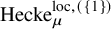 , so the claim follows from our observation.
To prove 2), we first prove that it holds for the trivial partition
$(J)$
 , namely

We observe that both sides are natural with respect to compositions of
$\zeta $
 . More precisely, let
$\zeta _1: I \longrightarrow J$
 and
$\zeta _2: J \longrightarrow K $
 be two maps between finite sets. Then we see immediately from the definition that

We have the following lemma for the naturality of the left-hand side of (8) with respect to
$\zeta $
 .
Lemma 3.4. We have a canonical identification

Proof. We first note that the projection

factorizes through

where

is the projection onto the first factor.
We have a commutative diagram

with the middle square being Cartesian. Then we have

where the last identification is the base-change isomorphism.
Therefore, if we have established the identification (8) for both
$\zeta _1$
 and
$ \zeta _2$
 , then

proving (8) for
$\zeta _2 \circ \zeta _1$
 .
We know that
$\zeta $
 can be written as a composition of simple degenerations and injections, that is, a simple degeneration is a surjective map collapsing only two elements, and a simple injection is an injective map adding only one element, and we have seen that it is enough to prove (8) for these two cases. Moreover, they can be written as the disjoint union of (the identity map on) a finite set with either
$\{1,2\} \twoheadrightarrow \{1 \}$
 or
$\emptyset \hookrightarrow \{1\}$
 . Using [Reference Fargues and ScholzeFS21, Proposition VI.10.3], we can further reduce to the case that
$\zeta $
 is either
$\{1,2\} \twoheadrightarrow \{1 \}$
 or
$\emptyset \hookrightarrow \{1\}$
 .
We check
$\{1,2\} \twoheadrightarrow \{1 \}$
 first. In this case,
$i_{\zeta }^{\mathrm {loc}}$
 is an isomorphism and
$p_{\zeta }^{\mathrm {loc}}$
 is the map

identifying
$\mathrm {Hecke}^{\mathrm {loc},(\{1\})}$
 with the substack of
$\mathrm {Hecke}^{\mathrm {loc},(\{1,2\})}$
 where the two legs are the same. We can assume that
$U= U_1 \boxtimes U_2$
 is decomposable. Then there is a canonical identification

where
$\Delta _{\zeta }: \hat {G} \hookrightarrow \hat {G}^2$
 is the diagonal map and U is a representation of
$\hat {G}^2$
 . This is because
$\Delta _{\zeta }^* U = U_1 \otimes U_2$
 and
$p_{\zeta }^*\mathscr {S}_U^{\mathrm {loc},(\{1,2\})}$
 is the convolution product of
$\mathscr {S}_{U_1}^{\mathrm {loc},(\{1\})}$
 and
$\mathscr {S}_{U_2}^{\mathrm {loc},(\{2\})}$
 (using that
$\mathscr {S}_U^{\mathrm {loc},(\{1,2\})}$
 is the fusion product of
$\mathscr {S}_{U_1}^{\mathrm {loc},(\{1\})}$
 and
$\mathscr {S}_{U_2}^{\mathrm {loc},(\{2\})}$
 ), see the paragraph following the proof of [Reference Fargues and ScholzeFS21, Proposition VI.9.4]. Then the identification follows from the geometric Satake ([Reference Fargues and ScholzeFS21, Theorem VI.11.1]).
Next, we assume that
$\zeta $
 is
$\emptyset \hookrightarrow \{1\}$
 . Then
$p_{\zeta }^{\mathrm {loc}}$
 is

the unique map to the final object, and

is the section of the structure map corresponding to the trivial modification, that is, the modification is an isomorphism. Then

where
$1$
 is the trivial representation (of either
$\hat {G}$
 or the trivial group
$\hat {G}^{\emptyset }$
 ). This follows from
$\mathscr {S}_{1}^{\mathrm {loc},(\emptyset )}$
 being the constant local system, and
$\mathscr {S}_1^{\mathrm {loc},(\{1\})}$
 being the constant local system supported on
$\mathrm {Hecke}^{\mathrm {loc},(\{1\})}_0$
 (by 1)). A general U is a direct sum of
$1$
 , so the identification follows.
Now for a general partition
$(J_1, \ldots , J_k)$
 , we have a diagram with Cartesian squares

and we can pull back the identification for the trivial partition to obtain the desired one.
For the comparison with Witt vector Hecke stacks, we note that when
$I=\{1\}$
 , it follows from the paragraph before [Reference ScholzeSch17, Proposition VI.7.5] and the proof of
$loc.cit.$
 that under the inclusion
$\mathrm {Perv}(\mathrm {Hecke}_{\mu ,s}^{\mathrm {loc},{(\{1\})}},\Lambda ) \subset D_{\text {\'{e}t}}(Gr_{\mu }^{W,\diamond \diamond }, \Lambda )$
 with
$\Lambda = \mathcal {O}_{\mathbb {Q}_\ell (\sqrt {q})}$
 (recall that
$\mathrm {Hecke}_{\mu ,s}^{\mathrm {loc},{(\{1\})}}=L^+G \setminus Gr_{\mu }^{W,\diamond \diamond }$
 ),

where
$X=Gr_{\mu }^W$
 is the Witt vector affine Grassmannian. Now we work with the general
$IC_{\mu _{\bullet }}$
 , recall that the construction of
$IC_{\mu _{\bullet }}$
 is by taking the twisted product of
$IC_{\mu _i}$
 on
$Gr_{\mu _{\bullet }}=\overset {\sim }{\boxtimes } \ Gr_{\mu _i}$
 , see [Reference Xiao and ZhuXZ17, Section 3.4.1]. By passing to Hecke stacks, this corresponds precisely to
$(\kappa _{(\{1\}, \ldots , \{n\}}^{\mathrm {loc},(\{1\}, \ldots , \{n\})})^* \underset {j}{\boxtimes } \mathscr {S}_{U_j}^{\mathrm {loc},(\{1\})}$
 , which is the definition of
$\mathscr {S}_U^{\mathrm {loc},(I_1,\ldots ,I_k)}$
 .
We also have the geometric Satake for global Hecke stacks.
Theorem 3.5 (Fargues–Scholze).
Let
$I $
 be a finite set, and
$\mu _{\bullet }$
 be a collection of dominant geometric cocharacters of G indexed by I. Let
$\{I_1, \ldots , I_k\}$
 be a partition of I. There is a natural functor

from the category of representations of
$\hat {G}^I$
 , the product of the dual group of G (with
$\overline {\mathbb {Q}}_\ell $
 -coefficient), to the category
$D_{\text {\'{e}t}}^b(\mathrm {Hecke}^{(I_1, \ldots , I_k)}, \overline {\mathbb {Q}}_\ell )$
 . It has the following properties.
1) If U is irreducible with highest weight
$\mu _{\bullet }$
 , then
$\mathscr {S}_U^{(I_1, \ldots , I_k)}$
 is supported on
$\mathrm {Hecke}_{\mu _{\bullet }}^{(I_1, \ldots , I_k)}$
 .
2) Let
$\zeta : I \rightarrow J$
 be a map of finite sets,
$(J_1, \ldots , J_k)$
 be a partition of J, and
$I_i = \zeta ^{-1}J_i$
 . Then there exists a canonical isomorphism

where

is defined in (1),

is the projection onto the first factor, and
$\Delta _{\zeta }: \hat {G}^J \rightarrow \hat {G}^I$
 is the map sending
$(g_j)_{j\in J}$
 to
$(g_{\zeta (i)})_{i\in I}$
 .
3) There is a canonical isomorphism

where

is the convolution map defined in (2).
4) Let
$(J_1, \ldots , J_l)$
 be a partition of I such that
$J_j = I_{i_j} \cup \ldots \cup I_{i_{j+1}-1}$
 for some partition
$1=i_1 < i_2 < \ldots < i_{l+1}= k+1$
 of
$k+1$
 . Then we have a canonical isomorphism

where

is defined in (3), and
$U_j$
 is a representation of
$\hat {G}^{J_j}$
 .
5) Let U be irreducible with highest weight
$\mu _{\bullet }$
 . Then the pullback of
$\mathscr {S}_U^{(\{1\}, \ldots , \{n\})}$
 restricted to
$\mathrm {Hecke}_{\mu _{\bullet }, s}^{(\{1\}, \ldots , \{n\})}$
 through the canonical map

is identified with the analytification of
$A_{\mu _{\bullet }}$
 as defined in theorem 3.3 (5).
More precisely, as in Appendix A.1, we have the complex of sheaves
$a_X^*c_X^*A_{\mu _{\bullet }}$
 on
$X=\mathrm {Hecke}^{\mathrm {loc}(m)}_{\mu _{\bullet }}$
 , which can be further viewed as a complex of sheaves on
$\mathrm {Hecke}^W_{\mu _{\bullet }}$
 through the identification in Appendix A.3, and this is canonically identified with the pullback of
$\mathscr {S}_U^{(\{1\}, \ldots , \{n\})}$
 along

6) There is a natural restriction map

along which the pullback of
$\mathscr {S}_U^{\mathrm {loc},(I_1,\ldots ,I_k)}$
 is identified with
$\mathscr {S}_U^{(I_1,\ldots ,I_k)}$
 . Moreover, the isomorphisms in 1) to 5) are compatible under this restriction map with the corresponding isomorphisms in Theorem 3.3 for local Hecke stacks.
Remark 3.6. We can state 3) for more general partitions on the target, at the cost of further complicating the notation. For example, we can consider the partial convolution map

sending

to

The special case as stated above suffices for our purposes.
Remark 3.7. We can refine the Theorem using Langlands L-groups, see [Reference Fargues and ScholzeFS21, Theorem VI.0.2]. More precisely, let
$\mathrm {Hecke}_{ \mathrm {Spd}(\mathbb {Z}_p)^I}^{(I_1,\ldots ,I_k)}$
 be the Hecke stack over
$\mathrm {Spd}(\mathbb {Z}_p)^I$
 , see remark 2.2. Then there is a functor from representations U of the L-group
$(^LG)^I$
 to complexes of sheaves
$\mathscr {S}_{U}^{(I_1,\ldots ,I_k)}$
 on
$\mathrm {Hecke}_{ \mathrm {Spd}(\mathbb {Z}_p)^I}^{(I_1,\ldots ,I_k)}$
 with properties similar to those in the Theorem, which refines the functor in the Theorem.
Proof. We define
$\mathscr {S}_U^{(I_1,\ldots ,I_k)}$
 as the pullback of
$\mathscr {S}_U^{\mathrm {loc},(I_1,\ldots ,I_k)}$
 along the canonical map

from global Hecke stacks to local Hecke stacks. Then (1), (2), (3), (4), and (6) follow immediately from the local version in Theorem 3.3.
For (5), we note that the composition of the canonical maps

is exactly the comparison map

in Appendix A.1 with
$X=\mathrm {Hecke}^{\mathrm {loc}(\infty )}_{\mu _{\bullet }}$
 , and the claim follows readily from Theorem 3.3 (5) and the identifications in Appendix A.3.
Now we study morphisms between the Satake sheaves
$\mathscr {S}_U^{(I_1,\ldots ,I_k)}$
 . We aim to interpret the morphisms as cohomological correspondences, similarly to [Reference Xiao and ZhuXZ17, Corollary 3.4.4]. The possibility of having multiple legs makes the situation more complicated.
Let U be a representation of
$\hat {G}^I$
 . We denote

where the index
$\mu _{\bullet }$
 ranges over the highest weights of irreducible summands of U. Similarly for
$\mathrm {Hecke}_{U|U'}^{(I_1, \ldots , I_k)|(J_1, \ldots , J_l), 0}$
 .
Proposition 3.8. Let
$I, J, K$
 be finite sets, and let
$\{I_1, \ldots , I_k\}$
 (resp.
$\{J_1, \ldots , J_l\}$
 ) be a partition of I (resp. J). Let
$\zeta : I \longrightarrow K$
 and
$\zeta ': J \longrightarrow K$
 be two maps.
Let U (resp.
$U'$
 ) be a representation of
$\hat {G}^I$
 (resp.
$\hat {G}^J$
 ). Then there is a natural map

where X is the space

and the right-hand side denotes the set of cohomological correspondences from

to

supported on X.
Let us first explain where the correspondence X comes from. The idea is that we want to complete the correspondence diagram

to a Cartesian square.
Observe that
$\mathrm {Hecke}_{U|U'}^{(I_1, \ldots , I_k)|(J_1, \ldots , J_l), 0} $
 lies over
 , and we want to use
$\zeta $
 and
$\zeta '$
 to pass to the same labeling set K; namely, we base change along

to obtain the diagram

Now there is a natural way to complete the diagram

and it is easy to see that it gives rise to a Cartesian square

Proof. We work on the derived level, and write
$p^!$
 and
$p_!$
 instead of
$Rf^!$
 and
$Rf_!$
 . From the Cartesian square (9), we compute


where the second identity holds because
$p_2$
 is proper, the third and the fifth identities are by proper base change, the second-to-last identity is 3) of Theorem 3.5 and the last identity is 2) of Theorem 3.5. Now geometric Satake ([Reference Fargues and ScholzeFS21, Theorem VI.11.1]) tells us that

which pulls back to morphisms in
$\mathrm {Hom}(\mathscr {S}_{\Delta _{\zeta }^*U}^{(K)}, \mathscr {S}_{\Delta _{\zeta '}^* U'}^{(K)})$
 , giving rise to the desired map

We document some special cases of the proposition, which are variants of the constructions in [Reference LafforgueLaf18, chapter 5].
Example 3.9. Let
$I=J$
 with the trivial partition
$(I)$
 ,
$K=\{1\}$
 , and
$\zeta =\zeta '$
 be the unique map from I to K. Let U and
$U'$
 be irreducible with highest weights
$\mu _{\bullet }$
 and
$\mu ^{\prime }_{\bullet }$
 . Then the proposition says that

If we further restrict the legs at the characteristic p untilt, then the support becomes
$\mathrm {Hecke}_{\Delta ^* U |\Delta ^* U',s}^{(\{1\})|(\{1\}),0}$
 , and this is a version of [Reference Xiao and ZhuXZ17, Corollary 3.4.4].
More precisely, the
$\diamond \diamond $
 -analytification of
$loc.cit.$
 is the version of (10) for local Hecke stacks (with fixed legs), and (10) is the pullback of the local version along the global-to-local map
$\mathrm {Hecke}^{(I)} \longrightarrow \mathrm {Hecke}^{\mathrm {loc}, (I)}$
 .
Example 3.10. (creation correspondences)
Let
$I= \{1,2\}$
 with partition
$(\{1\},\{2\})$
 ,
$J= \{1,2,3\}$
 with partition
$(\{1,2\},\{3\})$
 ,
$K=\{1,2\}$
 ,
$\zeta = \mathrm {id}$
 , and
$\zeta '= \begin {cases} \{1,3\} \rightarrow \{1\} \\ \{2\} \rightarrow \{2\} \end {cases}\!\!\!\!\!\!. $
 Let U and V be representations of
$\hat {G}$
 , and we consider

which parametrizes

More precisely, it parametrizes three legs labeled by 1, 2, and 3 with the legs labeled by 1 and 2 being the same.
$\varphi '$
 is a modification at the legs labeled by 1 and 2, with the modification at the leg labeled by 1 being trivial, and the leg labeled by 2 bounded by U.
$\varphi _1$
 is a modification at the two legs labeled by 1 and 2 with the one labeled by 1 being bounded by
$V^*$
 and the other bounded by U, and
$\varphi _2$
 is a modification at the leg labeled by 3 bounded by V.
The proposition then tells us that the canonical map

gives rise to a cohomological correspondence

supported on
$X $
 , where
$\sharp : 1 \rightarrow V^* \otimes V$
 is the canonical map sending 1 to the identity map in
$V^* \otimes V \cong \mathrm {Hom}(V,V)$
 .
In the application below, we will take a further base change along

where  is the section corresponding to the characteristic p untilt. Then we obtain

supported on

where we abuse notation by not distinguishing between
$\mathscr {S}_{ V^* \boxtimes U\boxtimes V}^{(\{1,2\},\{3\})}$
 as a sheaf on
$\mathrm {Hecke}_{ V^* \boxtimes U \boxtimes V}^{(\{1,2\},\{3\})}$
 and its pullback to
 . We hope the context will make it clear which support the sheaf lives on. Moreover, we have identified
 with
$\mathrm {Hecke}_{U}^{(\{1\})}$
 , which is clear.
Example 3.11 (annihilation correspondences).
Let
$I= \{1,2,3\}$
 with partition
$(\{1\},\{2,3\})$
 ,
$J= \{1,2\}$
 with partition
$(\{1\},\{2\})$
 ,
$K=\{1,2\}$
 ,
$\zeta = \begin {cases} \{1,2\} \rightarrow \{1\} \\ \{3\} \rightarrow \{2\} \end {cases}\!\!\!\!\!\!, $
 and
$\zeta '= \mathrm {id}$
 . Let U and V be representations of
$\hat {G}$
 , and we consider

The proposition then tells us that the canonical map

gives rise to a cohomological correspondence

supported on
$X $
 , where
$\flat : V \otimes V^* \rightarrow 1$
 is the evaluation map.
In the application below, we will take a further base change along

where  is the section corresponding to the characteristic p untilt, so we obtain

supported on

where we abuse notation by not distinguishing between
$\mathscr {S}_{ V \boxtimes V^* \boxtimes U}^{(\{1\},\{2,3\})}$
 as a sheaf on
$\mathrm {Hecke}_{V \boxtimes V^* \boxtimes U }^{(\{1\},\{2,3\})}$
 and its pullback to
 . We hope the context will make it clear which support the sheaf lives on. Moreover, we have identified
 with
$\mathrm {Hecke}_{U}^{(\{1\})}$
 , which is clear.
We will make use of the following simplified version of creation correspondences.
Example 3.12. Let
$I= \{1\}$
 with partition
$(\{1\})$
 ,
$J= \{1,2\}$
 with partition
$(\{1\},\{2\})$
 ,
$K=\{1\}$
 ,
$\zeta = \mathrm {id}$
 , and
$\zeta '$
 be the unique map from J to K. Let V be a representation of
$\hat {G}$
 , and we consider

which parametrizes

where
$\varphi _1$
 is a modification at an untilt bounded by
$V^*$
 , and
$\varphi _1$
 is a modification at the same untilt bounded by V.
We note that X is naturally identified with the closed substack

of
$\mathrm {Hecke}_{V^*\boxtimes V}^{(\{1\},\{2\})} $
 parametrizing

that is, it is the closed substack of
$\mathrm {Hecke}_{V^*\boxtimes V}^{(\{1\},\{2\})} $
 defined by the condition that
$\varphi _2 \circ \varphi _1$
 is an isomorphism. The correspondence diagram is then

where
$\pi $
 maps (13) to the isomorphism
$\varphi _2 \circ \varphi _1$
 , and i is the closed immersion.
The proposition then tells us that the canonical map

gives rise to a cohomological correspondence

supported on
$ \mathrm {Hecke}_{V^*\boxtimes V}^{(\{1\},\{2\}),0} $
 , where
$\sharp : 1 \rightarrow V^* \otimes V$
 is the canonical map sending 1 to the identity map in
$V^* \otimes V \cong \mathrm {Hom}(V,V)$
 .
In the application below, we will take a further base change along

where s is the section corresponding to the characteristic p untilt. Then we obtain the cohomological correspondence

supported on

where we abuse notation by not distinguishing between
$\mathscr {S}_{ V^* \boxtimes V}^{(\{1\},\{2\})}$
 (resp.
$\mathscr {S}_{ 1}^{(\{1\})}$
 ) as a sheaf on
$\mathrm {Hecke}_{ V^* \boxtimes V}^{(\{1\},\{2\})}$
 (resp.
$ \mathrm {Hecke}_{1}^{(\{1\})} $
 ) and its pullback to
$\mathrm {Hecke}_{ V^* \boxtimes V,s \times s}^{(\{1\},\{2\})} $
 (resp.
$ \mathrm {Hecke}_{1,s}^{(\{1\})} $
 ). We hope the context will make it clear which support the sheaf lives on.
The construction in the last example can be performed on local Hecke stacks. Note that, in the local case, it is important that we restrict to legs at the characteristic p untilt, as otherwise the correspondence Hecke stacks
$Hecke^{\mathrm {loc}, 0}_{1|V^*\otimes V}$
 need not exist, see remark 2.7.
Lemma 3.13.
(1) The canonical map
$\sharp : 1 \longrightarrow (V^* \otimes V) $
 gives rise to a cohomological correspondence

supported on

where
$\mathrm {Hecke}_{V^*\boxtimes V,s \times s}^{\mathrm {loc},(\{1\},\{2\}),0} $
 is the closed substack of
$\mathrm {Hecke}_{V^*\boxtimes V,s\times s}^{\mathrm {loc},(\{1\},\{2\})}$
 parametrizing

$\pi ^{\mathrm {loc}}$
 sends the data to the isomorphism
$\varphi _2 \circ \varphi _1$
 , and
$i^{\mathrm {loc}}$
 is the closed immersion.
(2)
$\mathscr {C}_{\sharp }^{+,0}$
 is the pullback of
$\mathscr {C}_{\sharp }^{\mathrm {loc},+,0}$
 along the diagram

(3) We have a cohomological correspondence on truncated Witt vector Hecke stacks

supported on

and we have

under the identification in Appendix A.3 between sheaves on truncated and untruncated moduli spaces of shtukas, that is,
$\mathscr {C}_{\sharp }^{\mathrm {loc},+,0}$
 is the
$\diamond \diamond $
 -analytification of
$\mathscr {C}_{\sharp }^{\mathrm {loc}(m,n),+,0}$
 , see Appendix A.2 for the notation.
Proof. As in the proof of Proposition 3.8, we have the Cartesian square

where
$\zeta : \{1,2\} \longrightarrow \{1\}$
 is the unique map. We can computeFootnote
5


where the fourth equality is the base-change isomorphism, the sixth equality is 3) of Theorem 3.3, the second-to-last equality is 1) and 2) of Theorem 3.3, and the last equality is the geometric Satake ([Reference Fargues and ScholzeFS21, Theorem VI.11.1]).
The construction given here is parallel to the construction in Proposition 3.8, and (2) follows from 6) of Theorem 3.5.
Lastly, (3) follows from 5) of Theorem 3.3. Indeed, it is a special case of [Reference Xiao and ZhuXZ17, Corollary 3.4.4].
Let us consider the correspondence

in Example 3.10, we note that if we restrict to the generic fiber, we have a canonical identification

where

is the substack parametrizing

with
$\varphi _1$
 and
$\varphi _2$
 bounded by (highest weights of irreducible summands of)
$V^*$
 and V respectively, and
$\varphi _3$
 bounded by
$\mu $
 . The correspondence diagram becomes

where the morphism p sends (18) to the first line

Lemma 3.14. The restriction of the cohomological correspondence
$\mathscr {C}_{\sharp }^+$
 in example 3.10 to the generic fiber, namely

supported on
$\mathrm {Hecke}_{ V^* \boxtimes U \boxtimes V,s \times s \times \eta }^{(\{1,2\},\{3\}),0}$
 , is canonically identified with the pullback of

along the diagram

Proof. We note that the diagram can be completed into

where
$i': \mathrm {Hecke}_{1,s}^{(\{1\})} \hookrightarrow \mathrm {Hecke}_{V^*\otimes V,s }^{(\{1\})} \cong \mathrm {Hecke}_{V^*\boxtimes V,s \times s}^{(\{1,2\})}$
 is the canonical closed immersion. We note that the lower square is Cartesian and is also the square used in the construction of
$\mathscr {C}_{\sharp }^{+,0} $
 (
$\boxtimes \mathrm {id}$
 ).
On the other hand, we have the Cartesian square

that is used in the construction of
$\mathscr {C}_{\sharp }^+$
 , where
$i":\mathrm {Hecke}_{1 \boxtimes U,s \times \eta }^{(\{1\},\{2\})} \hookrightarrow \mathrm {Hecke}_{V^*\boxtimes V\boxtimes U,s \times s \times \eta }^{(\{1,2,3\})} $
 is the map sending

to the composition

These two squares are compatible in the sense that we have a commutative cube

where f is the separating morphism sending

to

and

such that
$\varphi =\varphi _2 \circ \varphi _1$
 , where
$\varphi _1$
 is the modification at the characteristic p untilt, and
$\varphi _2$
 is the modification at the characteristic 0 untilt. Now the lemma follows readily from 4) of Theorem 3.5 and the construction of
$\mathscr {C}_{\sharp }^{+,0} $
 and
$\mathscr {C}_{\sharp }^{+} $
 .
4 The Hecke operators
In this section, we introduce the Hecke operators. We follow the same notations as above.
There is a canonical map

that sends a shtuka
$\{ \mathcal {P},\varphi _{\mathcal {P}}, S^{\sharp }\}$
 to
$\{\mathcal {P}, \mathrm {Frob}_S^*\mathcal {P}, \varphi _{\mathcal {P}},S^{\sharp }\}$
 , and we can use it to pull back the canonical sheaves in geometric Satake to sheaves on moduli spaces of shtukas.
Let U be an irreducible representation of
$\hat {G}$
 with highest weight
$\mu $
 . We have a diagram

where the last vertical map is the canonical restriction map. The square in the diagram is not commutative, but they become commutative after composing with the vertical map. Indeed, recall from Notation 2.16 that the legs of shtukas in the diagram are in characteristic zero, while the modification bounded by
$\nu $
 takes place at characteristic p; hence it does not affect the local type of
$\varphi _{\mathcal {P}}$
 , that is, the diagram is commutative after composing with the vertical map.
Now we have a cohomological correspondence
$\mathscr {C}_{\nu }$
 from
$(\mathrm {Sht}_{\mu ,\eta }, \epsilon _{\mu }^{(\{1\}),*}\mathscr {S}_U^{(\{1\})})$
 to itself supported on
$ \mathrm {Sht}^{\nu }_{\mu |\mu ,\eta }$
 , namely

where we use
$r^*\mathscr {S}_U^{\mathrm {loc},(\{1\})} =\mathscr {S}_U^{(\{1\})}$
 (see 6) of Theorem 3.5) and the étaleness of
$p_2$
 (Proposition 2.18) for the last isomorphism.
Now let V be a representation of
$\hat {G}$
 , and

be the function corresponding to V through the classical Satake equivalence

as defined in [Reference Xiao and ZhuXZ17, Section 3.5.2], where
$R(\hat {G}) := K_0(\mathrm {Rep}(\hat {G}))$
 is the representation ring of
$\hat {G}$
 , and
 is the space of compactly supported, that is, supported on a finite subset,
$\overline {\mathbb {Q}}_\ell $
 -valued functions on the double quotient set
 . Note that we use that G is unramified here, that is,
 is split, so the Langlands dual group of
 can be reduced to the dual group
$\hat {G}$
 . We know that
 has a basis indexed by dominant cocharacters
$\nu $
 (
$\mathcal {G}$
 is reductive over
$\mathbb {Z}_p$
 ), that is,
 ’s form a basis of
 , so
 with K a finite unramified extension of
$\mathbb {Q}_p$
 over which G splits. Let
$\Gamma _V$
 be the union of
$\mathrm {Sht}^{\nu }_{\mu |\mu ,\eta }$
 (as closed subspaces of
$\mathrm {Sht}^{}_{\mu |\mu ,\eta }$
 ) with
$\nu $
 appearing in
$h_V$
 . Then we define the Hecke operator
$T_V$
 as the cohomological correspondence that is supported on
$\Gamma _V$
 and is
$h_V(\nu (p))$
 times the cohomological correspondence (22) on
$\mathrm {Sht}^{\nu }_{\mu |\mu ,\eta }$
 . More precisely, we define

as a cohomological correspondence from
$(\mathrm {Sht}_{\mu ,\eta }, \epsilon _{\mu }^*\mathscr {S}_U)$
 to itself supported on

Note that if V is irreducible with highest weight
$\delta $
 , then
$h_V(\nu (p))\neq 0$
 precisely when
$\nu \leq \delta $
 , hence
$\Gamma _V= \mathrm {Sht}^{\nu }_{\mu | \mu ,\eta }$
 . Since
$\mathrm {Sht}^{\nu }_{\mu | \mu ,\eta } \subset \mathrm {Sht}^{\delta }_{\mu | \mu ,\eta }$
 as a closed substack, we can view
$\mathscr {C}_{\nu }$
 as being supported on
$\mathrm {Sht}^{\delta }_{\mu | \mu ,\eta }$
 , whence the sum in the definition of
$T_V$
 makes sense. In general,
$\Gamma _V$
 is the union of
$\mathrm {Sht}^{\delta }_{\mu | \mu ,\eta }$
 where
$\delta $
 ranges over highest weights of irreducible summands of V.
We observe that when
$\mu $
 is minuscule,
$\mathscr {S}_U = \overline {\mathbb {Q}}_\ell [d]$
 is the shifted constant sheaf with d being the dimension of the Schubert variety with respect to
$\mu $
 , and the cohomological correspondence
$\mathscr {C}_{\nu }$
 is the canonical isomorphism

We assume from now on that V is a representation of
$^LG$
 , which, by the proof of [Reference ZhuZhu15, Lemma A.3], is equivalent to a representation of
$\hat {G}$
 that we still denote by V, together with an isomorphism to its Frobenius twist
$^{\sigma } V$
 , where
$^{\sigma } V$
 is the representation of
$\hat {G}$
 obtained by twisting the action of G on V with the inverse Frobenius action on
$\hat {G}$
 , see [Reference Xiao and ZhuXZ17, Section 3.4.5]. Then the (unramified) classical Satake equivalence

defined in [Reference Xiao and ZhuXZ17, Section 3.5.2] provides us with
$h_V:= \mathrm {Sat}^{\mathrm {cl}} ([V]) \in C_c(G(\mathbb {Q}_p)//\mathcal {G}(\mathbb {Z}_p)), \overline {\mathbb {Q}}_\ell )$
 .
5 The excursion operators
We now start to define the excursion operators. We follow the same notation as in Section 4. In particular, let U be an irreducible representation of
$\hat {G}$
 with highest weight
$\mu $
 , and V be a representation of
$^LG$
 , viewed as a representation of
$\hat {G}$
 together with an isomorphism
$^{\sigma }V \cong V$
 with its Frobenius twist
$^{\sigma }V$
 .
We have a canonical map

which is simply viewing
$\mathrm {Frob}_S^*\mathcal {P}_1$
 as
$\mathcal {P}_{k+1}$
 . Similarly we have

which forms a commutative diagram

with the two squares Cartesian.
Let W be a representation of
$\hat {G}^I$
 . We denote

where the index
$\mu _{\bullet }$
 ranges over the highest weights of irreducible summands of W. Similarly for
$\mathrm {Sht}_{W|W'}^{(I_1, \ldots , I_k)|(J_1, \ldots , J_l), 0}$
 , and the Witt vector version.
5.1 The creation correspondences
First we define the creation correspondences.
Let
$\zeta : \{1\} \rightarrow \{1,2,3\} $
 be the map defined by
$\zeta (1)=2$
 . We define

as the closed v-substack parametrizing modifications

with the first line in
$\mathrm {Sht}_{U}$
 and the second line in

Moreover, the legs indexed by U in both the upper and lower modifications are the same.
Similarly, we define

as the v-substack parametrizing modifications

with the first line in
$\mathrm {Hecke}_{U}^{(\{1\})}$
 and the second line in

Moreover, the legs indexed by U in both the upper and lower modifications are the same.
We view
$\mathrm {Hecke}^{(\{1\})|(\{1,2\},\{3\}),0}_{U| V^* \boxtimes U \boxtimes V,-|s \times - \times s}$
 ,
$\mathrm {Sht}_{\mu |V^* \boxtimes U \boxtimes V,s \times - \times s}^{(\{1\})|(\{1,2\},\{3\}),0}$
 and
$\mathrm {Hecke}_{V^*\boxtimes U \boxtimes V, s \times - \times s }^{(\{1,2\},\{3\})}$
 as stacks over
 , and we have a commutative diagram over


Now since the squares in diagram (24) are Cartesian, we can pull back the cohomological correspondence

supported on
$\mathrm {Hecke}^{(\{1\})|(\{1,2\},\{3\}),0}_{U|V^* \boxtimes U \boxtimes V} $
 defined in Example 3.10 (11) to obtain the desired creation correspondence

supported on
$\mathrm {Sht}_{U|V^*\boxtimes U \boxtimes V, -| s \times - \times s}^{(\{1\})|(\{1,2\},\{3\}),0}$
 .
Remark 5.1. The reason we use
$\mathrm {Sht}_{V^* \boxtimes U \boxtimes V, s \times - \times s}^{(\{1,2\},\{3\})}$
 instead of
$\mathrm {Sht}_{ V^* \boxtimes U \boxtimes V, s \times - \times s}^{(\{1\},\{2\},\{3\})}$
 is explained in the paragraph before [Reference Xiao and ZhuXZ17, Remark 6.1.10], namely, we want the corresponding (integral) excursion operators to have the same support as the Hecke operators, so that we can pull back the cohomological correspondences to Shimura varieties.
5.1.1 The generic fiber
We now want to identify the generic fiber of the creation correspondences.
We first observe that
$\mathrm {Sht}_{V^*\boxtimes V\boxtimes U, s\times s \times \eta }^{(\{1\},\{2\},\{3\})}$
 is identified with the generic fiber of
$\mathrm {Sht}_{V^*\boxtimes U \boxtimes V, s \times \eta \times s }^{(\{1,2\},\{3\})}$
 , and similarly for
$\mathrm {Hecke}_{V^*\boxtimes V\boxtimes U, s\times s \times \eta }^{(\{1\},\{2\},\{3\})}$
 .
Lemma 5.2. There are natural identifications

and

Proof. When the two legs of
$\mathcal {P}_1 \dashrightarrow \mathcal {P}_2$
 are different, it is the same as the data of

where the first modification takes place at the characteristic p untilt, and the second over characteristic 0 untilts. Now as the two legs of

are different, and by Beauville–Laszlo it is the same as the data of

where the first modification takes place at the characteristic p untilt, and the second takes place at characteristic zero untilts. Similarly for
$\mathrm {Hecke}_{V^*\boxtimes U \boxtimes V, s \times \eta \times s }^{(\{1,2\},\{3\})}$
 .
Let
$\zeta : \{1\} \rightarrow \{1,2,3\}$
 be the map defined by
$\zeta (1)=3$
 , and

be the v-substack parametrizing modifications

with the first line in
$\mathrm {Sht}_{U,\eta }$
 and the second line in
$\mathrm {Sht}_{V^* \boxtimes V \boxtimes U,s \times s \times \eta }^{(\{1\},\{2\},\{3\})}$
 . Moreover, the legs indexed by U in both the upper and lower modifications are the same. In other words, it is the generic fiber of
$\mathrm {Sht}_{U|V^* \boxtimes U\boxtimes V ,- |s \times - \times s}^{(\{1\})|(\{1,2\},\{3\}),0}$
 under the identification in Lemma 5.2.
By our convention,
$\mathrm {Sht}_{U,\eta }$
 has its leg in characteristic zero, while the first two modifications of the second line take place at characteristic p. Hence the third modification takes place at the same leg as the first line, and the diagram is equivalent to

where the first two dashed arrows are modifications at the characteristic p untilt bounded by
$V^*$
 and V, respectively, whose composition is an isomorphism, and the last dashed arrow is a modification at characteristic zero untilts bounded by U. It means that
$\mathrm {Sht}_{U|V^*\boxtimes V \boxtimes U,-|s \times s \times -, \eta }^{(\{1\})|(\{1\},\{2\},\{3\}),0}$
 is a closed v-substack

of
$\mathrm {Sht}_{V^*\boxtimes V\boxtimes U,s \times s \times \eta }^{(\{1\},\{2\},\{3\})}$
 , which parametrizes diagrams as in (27) without the isomorphism condition, and the correspondence diagram becomes

where
$p_2$
 is the closed immersion, and
$p_1$
 sends (27) to the first row

The restriction of
$\mathscr {C}_{\sharp }$
 to the generic fiber then gives rise to the cohomological correspondence

supported on
$\mathrm {Sht}_{V^*\boxtimes V\boxtimes U,s\times s\times \eta }^{(\{1\},\{2\},\{3\}),0}$
 .
Lemma 5.3.
$\mathscr {C}_{\sharp ,\eta }$
 is the pullback of
$\mathscr {C}_{\sharp }^{\mathrm {loc},+,0} \boxtimes \mathrm {id}$
 defined in Lemma 3.13 (1) along the following diagram

where the maps between the last two rows are the global-to-local restriction maps (
$\times \mathrm {id}$
 ).
Proof. Clearly the squares are Cartesian, so we can pull back cohomological correspondences. By definition of
$\mathscr {C}_{\sharp }$
 , the restriction of
$\mathscr {C}_{\sharp }$
 to the generic fiber,

is the pullback of
$\mathscr {C}_{\sharp ,\eta }^+$
 defined in Lemma 3.14 along the first two rows.
By Lemma 3.14,
$\mathscr {C}_{\sharp }^+$
 is the pullback of
$\mathscr {C}_{\sharp }^{+,0} \boxtimes \mathrm {id}$
 along the middle two rows in the diagram.
Further, we know from Lemma 3.13 (2) that
$\mathscr {C}_{\sharp }^{+,0}$
 is the pullback of
$\mathscr {C}_{\sharp }^{\mathrm {loc},+,0}$
 along the global-to-local restriction maps. Thus
$\mathscr {C}_{\sharp , \eta }$
 is the pullback of
$\mathscr {C}_{\sharp }^{\mathrm {loc},+,0} \boxtimes \mathrm {id}$
 all the way from the bottom of the diagram.
The key observation for us is that the above diagram factorizes through moduli spaces of Witt vector shtukas.
Lemma 5.4. We have the following commutative diagram whose composition is the same as that of the diagram in Lemma 5.3,

where the vertical maps along the first lines are restrictions to the moduli spaces of local shtukas at the special fiber.
More precisely, the restriction map

in the diagram is a shtuka version of
$\kappa _{(\{1,2\},\{3\})}^{(\{1\},\{2\},\{3\})}$
 , namely sending

to
![P sub 1 restricted to Spec(O hat sub Y [0, infinity) (S), s) dashed arrow phi 1 to P sub 2 restricted to Spec(O hat sub Y [0, infinity) (S), s) dashed arrow phi 3 circle phi 2 to Frob super star sub S P sub 1 restricted to the same Spec domain.](https://static.cambridge.org/binary/version/id/urn:cambridge.org:id:binary:20261103013740893-0635:S2050509426102710:S2050509426102710_eqnu241.png?pub-status=live)
and
![Equation showing P sub 3 restricted to Spec(O hat Y [0, infinity) (S), S sharp) dashed arrow with phi sub 3 to Frob super star sub S P sub 1 restricted to Spec(O hat Y [0, infinity) (S), S sharp).](https://static.cambridge.org/binary/version/id/urn:cambridge.org:id:binary:20261103013740893-0635:S2050509426102710:S2050509426102710_eqnu242.png?pub-status=live)
and similarly for the other two. Since the modification
$\varphi _3$
 has its leg at characteristic 0 untilts, it is an isomorphism after restricting to
$\mathrm {Spec}(\mathcal {O}^{\wedge }_{\mathcal {Y}_{[0,\infty )}(S), S})$
 .
On the other hand, the map

is the forgetful map sending

to

with
$\mathcal {P}_{k+1}:= \mathrm {Frob}_S^*\mathcal {P}_1$
 .
Proof. Obvious.
Similar to the p-adic shtuka case, we can pull back
$\mathscr {C}_{\sharp }^{\mathrm {loc},+,0}$
 in (17) along

to obtain the Witt vector creation cohomological correspondence

supported on
$\mathrm {Sht}_{V^*\boxtimes V}^{\mathrm {loc}, W,0}$
 .
Proposition 5.5. The creation cohomological correspondence
$\mathscr {C}_{\sharp , \eta }$
 in (28) is naturally identified with the pullback of
$\mathscr {C}_{\sharp }^{\mathrm {loc},0,W} \boxtimes \mathrm {id}$
 along

Moreover,
$\mathscr {C}_{\sharp }^{\mathrm {loc},0,W}$
 is the
$\diamond \diamond $
 -analytification of the corresponding truncated Witt vector version as considered in [Reference Xiao and ZhuXZ17, example 6.1.9].
Proof. We use the truncated version of shtukas and Hecke stacks as defined in [Reference Xiao and ZhuXZ17, section 5.3] and recalled in Appendix A.3. The truncated perfect stacks as defined in Appendix A.3 can be defined directly in the world of v-stacks, either by writing out the obvious moduli problem or by taking the corresponding
$\diamond \diamond $
 -analytification.
We note that the truncated version of Diagram (29) is really the
$\diamond \diamond $
 -analytification of the diagram of perfect stacks below

which defines
$\mathscr {C}_{\sharp }^{\mathrm {loc}(m,n),0}$
 by pullback of
$\mathscr {C}_{\sharp }^{\mathrm {loc}(m),+,0}$
 . We know that
$\mathscr {C}_{\sharp }^{\mathrm {loc}(m),+,0,\diamond \diamond } = \mathscr {C}_{\sharp }^{\mathrm {loc},+,0}$
 so it follows from Proposition A.4 that

under the identification in Appendix A.3.
5.1.2 The special fiber
Lastly, we identify the creation correspondence at the special fiber. We want to prove that the pullback of
$\mathscr {C}_{\sharp }$
 (restricted to the special fiber) along the restriction map
$\mathrm {Sht}^W_{U} \longrightarrow \mathrm {Sht}_{U,s}$
 is precisely the
$\diamond \diamond $
 -analytification of the creation correspondence constructed in [Reference Xiao and ZhuXZ17, Example 6.1.9].
To simplify the notation, we denote

and

Similarly, we denote

and

As before, there is the diagram

where the vertical maps identify
$\mathcal {P}_{k+1}$
 as
$\mathrm {Frob}_S^*\mathcal {P}_1$
 .
On the other hand, we have the map

which is the restriction of moduli spaces of shtukas from
$W(R^+)$
 to
$\mathcal {Y}_{[0,\infty )}(S)$
 , and similarly for
$\mathrm {Sht}_{\mu _{\bullet }|\mu _{\bullet }}^{0,W}$
 . They form a commutative diagram

The Diagram (24) restricted to the special fiber is

We can compose it with the previous one to obtain

and we want to understand the pullback of the (restriction to the special fiber of) creation correspondence
$\mathscr {C}_{\sharp }$
 in (25) along the upper half of the diagram. We note that the diagram factorizes as

where the vertical maps of the second row are restrictions of torsors from
$W(R^+)$
 to
$\mathcal {Y}_{[0,\infty )}(R,R^+)$
 .
We can pull back the cohomological correspondence
$\mathscr {C}_{\sharp }^+$
 (restricted to the special fiber) defined in Example 3.10 (11) along the last diagram, which defines the creation correspondence on the global Witt vector shtuka

The importance of
$\mathscr {C}_{\sharp }^{W}$
 is that it is the
$\diamond \diamond $
 -analytification of the creation correspondence on moduli spaces of Witt vector shtukas constructed in [Reference Xiao and ZhuXZ17, Example 6.1.9].
Proposition 5.6.
$\mathscr {C}_{\sharp }^{W}$
 is the pullback of the restriction of the creation correspondence
$\mathscr {C}_{\sharp }^+$
 in (25) to
$\mathrm {Spd}(\overline {\mathbb {F}_p})$
 along

Moreover, we have

the analytification of the creation correspondence in [Reference Xiao and ZhuXZ17, Example 6.1.9].
Proof. The factorization (30) tells us that
$\mathscr {C}_{\sharp }^{W} $
 is the pullback of the creation correspondence (25) along

Next, we observe that the restriction of
$\mathscr {C}_{\sharp }^+$
 , as defined in Example 3.10 (11), to the special fiber has a local counterpart
$\mathscr {C}_{\sharp }^{\mathrm {loc},+}$
 , and
$\mathscr {C}_{\sharp }^+$
 is the pullback of
$\mathscr {C}_{\sharp }^{\mathrm {loc},+}$
 along the canonical restriction diagram

The restriction to the special fiber is important here, as otherwise
$\mathrm {Hecke}^{\mathrm {loc},(\{1\})|(\{1,2\},\{3\}),0}_{U| V^* \boxtimes U \boxtimes V,s} $
 does not exist; see Remark 2.7. As always,
$\mathscr {C}_{\sharp }^{+}$
 being the pullback of
$\mathscr {C}_{\sharp }^{\mathrm {loc},+}$
 follows ultimately from 6) of Theorem 3.5. Now we can compose the Diagram (31) with the above restriction diagram and obtain

and
$\mathscr {C}_{\sharp }^{W}$
 is the pullback of
$\mathscr {C}_{\sharp }^{\mathrm {loc},+}$
 along the diagram. Up to truncation, this is precisely

see Appendix A.1 for the notation of
$a_{?}$
 , and A.3 for the truncated Witt vector Hecke stacks and moduli spaces of Witt vector shtukas. We know from Appendix A.3 that the truncated version does not affect cohomology, so we can naturally view the cohomological correspondences on the (analytification of) truncated Witt vector Hecke stacks or moduli spaces of Witt vector shtukas as being defined on the untruncated ones.
We can perform the same construction as that of
$\mathscr {C}_{\sharp }^+$
 (in the theory of perfect stacks) to obtain

supported on

which is precisely the creation correspondence constructed in [Reference Xiao and ZhuXZ17, Example 6.1.9]. Now 6) of Theorem 3.5 (and the comparison results in appendices A.1 and A.2) tells us that

under the identification of sheaves on truncated and untruncated Hecke stacks in A.3. By definition of
$\mathscr {C}_{\sharp }^{\mathrm {loc}(m),+,\diamond }$
 , see Appendix A.2, and
$\mathscr {C}_{\sharp }^{+}$
 being the pullback of
$\mathscr {C}_{\sharp }^{\mathrm {loc},+}$
 , we have

Then the commutation between the analytification and pullback of cohomological correspondences (Proposition A.4) tells us that

again under the identification of sheaves on truncated and untruncated Witt vector Hecke stacks and moduli spaces of Witt vector shtukas, where
$\mathscr {C}_{\sharp }^{\mathrm {loc}(m,n)}$
 is the pullback of
$\mathscr {C}_{\sharp }^{\mathrm {loc}(m)}$
 along

As usual, we use
$\epsilon _?$
 to denote the (in the sense of perfect stacks) forgetful map (viewing the Frobenius twist of
$\mathcal {P}_1$
 as
$\mathcal {P}_2$
 ).
$\mathscr {S}_{\sharp }^{\mathrm {loc}(m,n)}$
 is exactly the construction of the creation correspondence on moduli spaces of Witt vector shtukas in [Reference Xiao and ZhuXZ17, Example 6.1.9], so we have proved that
$\mathscr {C}_{\sharp }^W$
 is the analytification of the creation correspondence in
$loc.cit$
 .
5.2 The annihilation correspondences
Dually, we have the annihilation correspondences.
Let
$\zeta : \{1\} \longrightarrow \{1,2,3\}$
 be a map defined by
$\zeta (1)=3$
 , and

be the v-substack parametrizing modifications

with the first line in

and the second line in
$\mathrm {Sht}_{U}^{(\{1\})}$
 . Moreover, the legs indexed by
$\mu $
 on the first and the second rows are the same.
Similarly, let

be the v-substack parametrizing modifications

with the first line in

and the second line in
$\mathrm {Hecke}_{U}^{(\{1\})}$
 . Moreover, the legs indexed by U on the first and the second rows are the same.
The annihilation correspondence is defined to be the cohomological correspondence

supported on
$\mathrm {Sht}_{ V \boxtimes V^* \boxtimes U| U, s\times s\times - |-}^0$
 that is the pullback of

defined in example 3.11 along

5.2.1 The generic fiber
We can identify the generic fiber of the annihilation correspondence, which is

supported on

As before, we have the local Witt vector version, that is, the cohomological correspondence

supported on

corresponding to the evaluation map

Proposition 5.7. The annihilation cohomological correspondence
$\mathscr {C}_{\flat }$
 of (35) is naturally identified with the pullback of


along the restriction diagram

Moreover,
$\mathscr {C}_{\flat }^{\mathrm {loc},0,W}$
 is the
$\diamond \diamond $
 -analytification of the corresponding truncated Witt vector version
$\mathscr {C}_{\flat }^{\mathrm {loc}(m,n),0}$
 constructed in [Reference Xiao and ZhuXZ17, Example 6.1.9].
Proof. The proof is the same as that of Proposition 5.5.
5.2.2 The special fiber
We can identify the annihilation correspondence at the special fiber as well.
Proposition 5.8.
$\mathscr {C}_{\flat }^{W}$
 is the pullback of the restriction of the annihilation correspondence (33) to
$\mathrm {Spd}(\overline {\mathbb {F}_p})$
 along the diagram

where

is the pullback of (34) (restricted to
$\mathrm {Spd}(\overline {\mathbb {F}_p})$
 ) along

Moreover,
$\mathscr {C}_{\flat }^W$
 is the analytification of the annihilation correspondence in [Reference Xiao and ZhuXZ17, Example 6.1.9], that is,

under the identification in A.2 between sheaves on truncated and untruncated moduli spaces of Witt vector shtukas.
Proof. The proof is the same as that of Proposition 5.6.
5.3 The partial Frobenius
Lastly, we define the partial Frobenius morphism. Let
$ \boxtimes U_i$
 be a representation of
$\hat {G}^I$
 , with each
$U_i$
 a representation of
$\hat {G}^{I_i}$
 . Moreover, we assume that
$U_1$
 is a representation of
$(^L G)^{I_1}$
 , so
$U_1$
 is isomorphic to its Frobenius twist
$^{\sigma }U_1$
 , and we fix such an isomorphism from now on.
We define the partial Frobenius to be the map

sending

to

Note that we have used the assumption on
$U_1$
 so that
$\mathrm {Frob}_S^*\varphi _1$
 is still bounded by
$U_1$
 . In general,
$\mathrm {Frob}_S^*\varphi _1 $
 would be bounded by
$^{\sigma }U_1$
 .
We have a commutative diagram

We have a canonical isomorphism

from which we obtain


where the first and the last isomorphisms are 4) of Theorem 3.5. It defines a pullback cohomological correspondence

supported on

Similarly, we have a partial Frobenius on moduli spaces of local Witt vector shtukas,

sending

to

where we view each
$U_i$
 as a representation of
$\hat {G}$
 through the diagonal embedding
$\hat {G} \hookrightarrow \hat {G}^{I_i}$
 .
There is a commutative diagram

As in the case of moduli spaces of shtukas, the diagram induces a pullback cohomological correspondence

supported on

which is the
$\diamond \diamond $
 -analytification of the partial Frobenius correspondence constructed in [Reference Xiao and ZhuXZ17, Lemma 6.1.11], namely,

under the identification in A.3 between sheaves on truncated and untruncated moduli spaces of Witt vector shtukas, where
$\mathscr {C}_{F}^{\mathrm {loc}(m,n)}$
 is the partial Frobenius cohomological correspondence considered in [Reference Xiao and ZhuXZ17, Lemma 6.1.11]. Note that the inverse of the partial Frobenius is used in
$loc.cit.$
 as it is better suited to the truncated moduli spaces of Witt vector shtukas. After passing to the analytic untruncated version, it agrees with our construction.
We now specialize to the situation that is relevant to us.
Example 5.9. We consider

Note that we have used our assumption that V is a representation of
$^LG$
 here. We have the partial Frobenius cohomological correspondence

supported on

If we restrict to the generic fiber, then under the identification in Lemma 5.2, we have

supported on

We want to relate it to the local Witt vector partial Frobenius correspondence

supported on

As usual, this is the
$\diamond \diamond $
 -analytification of the corresponding truncated Witt vector version
$\mathscr {C}_F^{\mathrm {loc}(m,n),0}$
 .
Proposition 5.10. The cohomological correspondence
$\mathscr {C}_{F,\eta }$
 is the same as the pullback of
$\mathscr {C}_F^{\mathrm {loc},0,W} \boxtimes \mathrm {id}$
 along the diagram

where the vertical arrows are, as before, restriction maps.
Moreover,

being the
$\diamond \diamond $
 -analytification of the truncated Witt vector version considered in [Reference Xiao and ZhuXZ17, Lemma 6.1.11].
Proof. It is clear that the two squares in the diagram are Cartesian, so we can pull back cohomological correspondences. We have the commutative diagram

where the bottom vertical maps are global-to-local restriction maps. We observe that it factorizes through

where the top vertical arrows are restriction maps, and the proposition follows from the construction of
$\mathscr {C}_F$
 and
$\mathscr {C}_F^{\mathrm {loc},W}$
 . Note that in the construction of
$\mathscr {C}_F$
 , we can also use the local Hecke stacks.
Lastly, we want to identify the special fiber of the partial Frobenius
$\mathscr {C}_F$
 , that is,

supported on

We first define the partial Frobenius on moduli spaces of Witt vector shtukas. As in the other two cases, it is defined to be

sending

to

We have the commutative diagram

which factorizes as

The last diagram defines the Witt vector partial Frobenius correspondence


which, as before, is the
$\diamond $
 -analytification of the partial Frobenius correspondence constructed in [Reference Xiao and ZhuXZ17, Lemma 6.1.11].
Now the Diagram (39) tells us that
$\mathscr {C}_F^{W} $
 is the pullback of
$\mathscr {C}_{F,s}$
 along the first square of (39). Specializing to the case of our interest, we have
Proposition 5.11. The correspondence


supported on

is the pullback of
$\mathscr {C}_{F,s}$
 along the diagram

Moreover,
$\mathscr {C}_{F}^W$
 is the
$\diamond $
 -analytification of the partial Frobenius cohomological correspondence considered in [Reference Xiao and ZhuXZ17, Lemma 6.1.11].
5.4 The excursion operators
We can now define the excursion operator associated to V as the cohomological correspondence

from
$(\mathrm {Sht}_{\mu }, \epsilon _{\mu }^{(\{1\}),*} \mathscr {S}_U^{(\{1\})})$
 to itself supported on

where
$\nu $
 ranges over the highest weights of the irreducible components of V. Indeed, we have
Lemma 5.12. The support of
$S_V$
 is
$\mathrm {Sht}_{\mu | \mu }^{V}$
 .
Proof. By definition, the support of
$S_V$
 is the fiber product of

which by definition parametrizes

where the upper-left triangle lies in
$\mathrm {Sht}_{V\boxtimes V^*\boxtimes U | U}^{0}$
 , and the lower-right triangle lies in
$\mathrm {Sht}_{U| V^*\boxtimes U \boxtimes V}^{0}$
 . In other words,
$\varphi _1$
 has a leg at the characteristic p untilt and is bounded by V, the two horizontal modifications have legs varying in
 and are bounded by U, while the diagonal one has two legs, with one fixed at characteristic p untilt bounded by
$V^*$
 , and the other varying in
 bounded by U. This is then the same as

with the two lines lying in
$\mathrm {Sht}_{\mu }$
 and
$\varphi _1$
 bounded by V, which is nothing but what
$\mathrm {Sht}_{\mu | \mu }^{V} $
 parametrizes. Indeed, the diagonal is just
$\psi \circ \varphi _1^{-1}$
 , and the modification takes place at the legs of
$\varphi _1$
 and
$\psi $
 , bounded by the corresponding cocharacters of
$\varphi _1^{-1}$
 and
$\psi $
 .
Note that we have

Thus
$S_V$
 restricted to
$\mathrm {Sht}_{\mu ,\eta }$
 is supported on
$\Gamma _V$
 , the same as the support of the Hecke correspondence.
Similarly, we have the local Witt vector version of the cohomological correspondence

from
$(\mathrm {Sht}_{0}^{\mathrm {loc},W}, \epsilon _{0}^{\mathrm {loc},(\{1\}),*} \mathscr {S}_1^{\mathrm {loc},(\{1\})})$
 to itself supported on
$\Gamma _V^{\mathrm {loc},W}$
 , which can be identified with
$ \mathrm {Sht}^{\mathrm {loc},V, W}_{0|0}$
 . Indeed, as in the proof of the previous lemma, we have that the support of
$S_V^{\mathrm {loc},0,W}$
 parametrizes diagrams

which is nothing but

whence
$\Gamma _V^{\mathrm {loc},W} = \mathrm {Sht}^{\mathrm {loc},V, W}_{0|0} $
 .
Theorem 5.13. The cohomological correspondence
$S_{V,\eta }$
 , the restriction of
$S_V$
 to
$\mathrm {Sht}_{\mu ,\eta }$
 , is the pullback of


along the diagram

where the vertical arrows are restriction maps; in particular, the middle one sends

to
![P sub 1 restricted to Spec(O hat Y [0, infinity) (S), S) dashed arrow with gamma restricted to Spec(O hat Y [0, infinity) (S), S) above it pointing to P sub 2 restricted to Spec(O hat Y [0, infinity) (S), S)](https://static.cambridge.org/binary/version/id/urn:cambridge.org:id:binary:20261103013740893-0635:S2050509426102710:S2050509426102710_eqnu336.png?pub-status=live)
and
![Script P sub 1 restricted to Spec of O-hat sub Y [0, infinity) (S), S-sharp dashed arrow with phi sub 1 maps to Frob super asterisk sub S Script P sub 1 restricted to Spec of O-hat sub Y [0, infinity) (S), S-sharp.](https://static.cambridge.org/binary/version/id/urn:cambridge.org:id:binary:20261103013740893-0635:S2050509426102710:S2050509426102710_eqnu337.png?pub-status=live)
Moreover,
$S_V^{\mathrm {loc},0,W}$
 is the
$\diamond \diamond $
 -analytification of

the truncated Witt vector excursion operator in [Reference Xiao and ZhuXZ17, Theorem 6.0.1 (1)].
Proof. Since we know that the pullback of cohomological correspondences respects composition, the Theorem follows from propositions 5.5, 5.7, and 5.10.
Remark 5.14. The Theorem holds with
$\mathrm {Sht}_{\mu ,\eta }$
 replaced by arbitrary
$\mathrm {Sht}_{\mu _{\bullet },\eta }^{(I_1, \ldots , I_k)}$
 . The proof goes without change. We state it only for shtukas with a single leg to simplify the notation and that is the only case that matters for Shimura varieties.
Lastly, we want to study the excursion operators at the special fiber. We have the global Witt vector excursion operator, which is the composition of (32), (40) and (36), that is,

is the cohomological correspondence from
$(\mathrm {Sht}^{W}_{\mu }, \epsilon _{\mu }^{W,*} r_{\mu }^* \mathscr {S}_U^{(\{1\})})$
 to itself supported on
$\mathrm {Sht}_{\mu | \mu }^{V, W}$
 .
Proposition 5.15.
$S_V^{W}$
 is the pullback of
$S_{V,s}$
 along

Moreover,
$S_V^W$
 is the analytification of the truncated Witt vector excursion operator considered in [Reference Xiao and ZhuXZ17], under the equivalence between sheaves on truncated and untruncated moduli spaces of Witt vector shtukas in A.3.
Proof. As
$\mathscr {C}_{\sharp }^W$
 ,
$\mathscr {C}_{F}^W$
 and
$\mathscr {C}_{\flat }^W$
 are all analytifications of the truncated Witt vector counterpart considered in [Reference Xiao and ZhuXZ17], so is the composite
$S_V^W$
 by Proposition A.4. Then Proposition 5.11, Proposition 5.8 and Proposition 5.6 tell us that
$S_V^{W}$
 is the pullback of
$S_{V,s}$
 , the restriction of
$S_V$
 to the special fiber.
6
$\boldsymbol{S=T}$
 for moduli spaces of shtukas

Let us first look more closely at
$S_V^{\mathrm {loc},W}$
 . Recall that it is supported on
$\Gamma _V^{\mathrm {loc},W} = \mathrm {Hecke}_V^{\mathrm {loc}} = L^{+,W}\mathcal {G} \setminus \text {Gr}^W_{G, \leq V}$
 , where
$L^{+,W}\mathcal {G}$
 is the v-sheaf whose value at a characteristic p affinoid perfectoid space
$\text {Spa}(R,R^+)$
 is
$\mathcal {G}(W(R))$
 , and
$\text {Gr}^W_{G, \leq V}$
 is the analytification of the Witt vector Schubert variety.
Similar to Hecke operators on
$\mathrm {Sht}_{\mu ,\eta }$
 , we also have them on
$\mathrm {Sht}_0^{\mathrm {loc},W}$
 . There is the diagram

Lemma 6.1.
$p_1$
 and
$p_2$
 are finite étale.
Proof. Given a morphism
$\text {Spa}(R,R^+) \rightarrow \mathrm {Sht}^{\mathrm {loc},W}_0$
 from an affinoid characteristic p perfectoid space into
$\mathrm {Sht}_0^{\mathrm {loc},W}$
 , determined by the data

its fiber product with
$p_2$
 is the (analytification of) refined Witt vector affine Deligne-Lusztig variety
$X^W_{0,\nu }(1)$
 Footnote
6
(base change to R), which parametrizes

with
$\gamma $
 bounded by
$\nu $
 (the second line is fixed). This can also be characterized as the fiber product

where a sends the above diagram to
$\gamma \varphi _1^{-1}$
 , b maps it to
$\gamma $
 and
$\varphi _2^{-1} \mathrm {Frob}$
 is the map sending
$\gamma : \mathcal {P}_1 \dashrightarrow \mathcal {P}_2$
 to
$\varphi _2^{-1}\mathrm {Frob}_S^*\gamma $
 (fixing a trivialization of
$\mathcal {P}_2$
 ). Since
$\varphi _2$
 is an isomorphism, we see that
$X^W_{0,\nu }(1) \cong Gr_{\nu }^W(\mathbb {F}_p)$
 as zero-dimensional varieties, which is obviously finite étale. Thus
$p_2$
 is finite étale, and similarly for
$p_1$
 .
Moreover, we see that

which can be identified with the substack

defined by the bounded-by-
$\nu $
 condition. Moreover, we have
$\mathrm {Sht}_0^{\mathrm {loc},W} = L^{+,W}\mathcal {G} \setminus \bullet $
 and
$\mathscr {S}_1^{(\{1\})}= \overline {\mathbb {Q}}_\ell $
 , so any function
$f \in C(\Gamma _{\nu }^W, \overline {\mathbb {Q}}_\ell ) $
 defines a cohomological correspondence
$\mathscr {C}_f^{\mathrm {loc},W}$
 from
$(\mathrm {Sht}_{0}^{\mathrm {loc},W}, \epsilon _{0}^{(\{1\}),*}\mathscr {S}_1^{\mathrm {loc},(\{1\})})$
 to itself supported on
$\Gamma _{\nu }^{\mathrm {loc},W}$
 which is multiplication by
$f(x)$
 at
$x \in \Gamma _{\nu }^{\mathrm {loc},W}$
 . See [Reference Xiao and ZhuXZ17, Proposition 5.4.4] for more details.
We can do the same construction with truncated moduli spaces of Witt vector shtukas as in [Reference Xiao and ZhuXZ17] to obtain
$\mathscr {C}_{f}^{\mathrm {loc}(m,n)}$
 , and we have

under the identification between sheaves on truncated and untruncated moduli spaces of Witt vector shtukas in Appendix A.3. Note that this identification only holds at the sheaf level, and not at the space level.
We have
$\Gamma _V^{\mathrm {loc},W} = \cup \Gamma _{\nu }^{\mathrm {loc},W}$
 where
$\nu $
 ranges over highest weights of irreducible summands of V, and we can similarly define
$\mathscr {C}_f^{\mathrm {loc},W}$
 for
$f \in C(\Gamma _{V}^{\mathrm {loc},W}, \overline {\mathbb {Q}}_\ell )$
 and

as cohomological correspondence from
$(\mathrm {Sht}_{0}^{\mathrm {loc},W}, \epsilon _{0}^{\mathrm {loc},(\{1\}),*}\mathscr {S}_1^{\mathrm {loc},(\{1\})})$
 to itself supported on
$\Gamma _{V}^{\mathrm {loc},W}$
 , where
$h_V$
 is the function corresponding to V under the classical Satake isomorphism. Similarly, we can define
$T_V^{\mathrm {loc}(m,n)} = \mathscr {C}_{h_V}^{\mathrm {loc}(m,n)}$
 , and we have

under the canonical identification in A.3 between sheaves on truncated and untruncated moduli spaces of Witt vector shtukas.
Theorem 6.2. (Xiao–Zhu)
We have an equality

as cohomological correspondence from
$(\mathrm {Sht}_{0}^{\mathrm {loc},W}, \epsilon _{0}^{\mathrm {loc},(\{1\}),*}\mathscr {S}_1^{\mathrm {loc},(\{1\})})$
 to itself supported on
$\Gamma _{V}^{\mathrm {loc},W}$
 .
Proof. This is the analytification of [Reference Xiao and ZhuXZ17, Theorem 6.0.1 (2)]. More precisely, Xiao–Zhu prove the equality as cohomological correspondences on perfect stacks, and we take the
$\diamond \diamond $
 -analytification of the corresponding cohomological correspondences to get an equality of cohomological correspondences on v-stacks. The comparison results (between cohomological correspondences on perfect stacks and their
$\diamond \diamond $
 -analytification) we proved in Section 5, recalled in the previous paragraph, tell us that the cohomological correspondences obtained by analytification coincide with the ones in the statement of the Theorem.
We can now prove the desired
$S=T$
 Theorem for moduli spaces of p-adic shtukas.
Theorem 6.3. There is a canonical identification

as cohomological correspondence from
$(\mathrm {Sht}_{\mu ,\eta }, \epsilon _{\mu }^{(\{1\}),*}\mathscr {S}_U^{(\{1\})})$
 to itself supported on
$\Gamma _V$
 .
Remark 6.4. Again, there is no difficulty generalizing the Theorem to shtukas with several legs (in characteristic zero).
Proof. Theorems 5.13 and 6.2 together imply that
$S_{V,\eta }$
 is the pullback of
$T_V^{\mathrm {loc},W} \boxtimes \text {id}$
 along

which is the same as
$T_V$
 . Indeed, we have a commutative diagram with the upper two squares Cartesian

where we abuse notation by writing
$\epsilon _{0}^{\mathrm {loc},(\{1\})}$
 for the unique map from
$\mathrm {Sht}_{0}^{\mathrm {loc},W}$
 to the final point
$*$
 . Then under the canonical identification
$* \times \mathrm {Hecke}_{\mu ,\eta }^{\mathrm {loc},(\{1\})} = \mathrm {Hecke}_{\mu ,\eta }^{\mathrm {loc},(\{1\})}$
 , the composition is precisely (21). Let
$\mathscr {C}_{\nu }^{\mathrm {loc},W} = \mathscr {C}_{1_{\Gamma _{\nu }^W}}^{\mathrm {loc},W}$
 with
$1_{\Gamma _{\nu }^{\mathrm {loc},W}}$
 the characteristic function of
$\Gamma _{\nu }^{\mathrm {loc},W}$
 . Then the pullback of
$\mathscr {C}_{\nu }^{\mathrm {loc},W} \boxtimes \text {id}$
 is

Using the fact that
$p_2$
 and
$p_2^{\mathrm {loc}}\times \text {id}$
 are étale, we see that

is nothing but


thus the pullback of
$\mathscr {C}_{\nu }^{\mathrm {loc},W} \boxtimes \text {id}$
 is simply
$\mathscr {C}_{\nu }$
 , hence the pullback of
$T_V^{\mathrm {loc},W}\boxtimes \text {id}$
 is
$T_V$
 by adding them together.
7
$\boldsymbol{S=T}$
for Shimura varieties

In this section, we assume that
$G / \mathbb {Q}$
 is a reductive group equipped with a
$G_{\mathbb {R}}$
 -conjugacy class X of homomorphisms
$h: \text {Res}_{\mathbb {C}/\mathbb {R}} \mathbb {G}_m \rightarrow G_{\mathbb {R}}$
 that gives rise to a Hodge-type Shimura variety. Namely, there is a closed embedding
$G \hookrightarrow \text {GSp}(Q, \psi )$
 such that X is mapped to the canonical Siegel conjugacy class, where Q is a finite-dimensional
$\mathbb {Q}$
 -vector space,
$\psi $
 is a nondegenerate alternating form on Q, and
$\text {GSp}(Q, \psi )$
 is the similitude symplectic group with respect to
$(Q, \psi )$
 , that is, the automorphism of Q preserving
$\psi $
 up to a constant. We fix such an embedding throughout. Then, by [Reference DeligneDel82], there is a set of tensors
$(s_{\alpha }) $
 in

such that G is the stabilizer of
$(s_{\alpha })$
 , which we also fix from now on.
We can base change h to
$\mathbb {C}$
 to obtain
$h_{\mathbb {C}}: \mathbb {G}_m \times \mathbb {G}_m \rightarrow G_{\mathbb {C}}$
 , where the two factors
$\mathbb {G}_m$
 correspond to the identity embedding and the conjugation embedding respectively. Let
$\mu : \mathbb {G}_m \rightarrow G_{\mathbb {C}}$
 be the restriction of
$h_{\mathbb {C}}$
 to the first factor, whose conjugacy class has field of definition E, which is a number field.
Moreover, we fix a prime p such that G is hyperspecial at p, that is, there is a reductive group
$\mathcal {G}$
 over
$\mathbb {Z}_{(p)}$
 with generic fiber G. Let
$K=K^p K_p \subset G(\mathbb {A}_f)$
 be a compact open subgroup where
$K_p = \mathcal {G}(\mathbb {Z}_p) \subset G(\mathbb {Q}_p)$
 and
$K^p \subset G(\mathbb {A}^p_f)$
 are compact open. We assume that
$K^p$
 is neat for convenience, so that the corresponding Shimura variety is a scheme instead of a stack. By enlarging Q, we may assume that Q has a lattice
$Q_{\mathbb {Z}_{(p)}}$
 over
$\mathbb {Z}_{(p)}$
 on which
$\psi $
 induces a perfect pairing
$Q_{\mathbb {Z}_{(p)}} \times Q_{\mathbb {Z}_{(p)}} \rightarrow \mathbb {Z}_{(p)}$
 . Moreover, we can assume that the embedding
$G \hookrightarrow \text {GSp}(Q, \psi )$
 induces an embedding

as reductive groups over
$\mathbb {Z}_{(p)}$
 , and the tensors
$s_{\alpha }$
 ’s extend to tensors of
$Q_{\mathbb {Z}_{(p)}}$
 whose stabilizer group is
$\mathcal {G}$
 , see [Reference KisinKis10, Section 2.3.2] for details.
By [Reference KisinKis10, Lemma 2.1.2], there is a compact open subgroup
$\tilde {K}^p \subset \text {GSp}(Q, \psi )(\mathbb {A}_f^p)$
 such that
$K^p = \tilde {K}^p \cap G(\mathbb {A}_f^p)$
 , and the injection of G into
$\text {GSp}(Q, \psi )$
 induces a closed embedding

of Shimura varieties, where
$\tilde {K}_p := \text {GSp}(Q_{\mathbb {Z}_{(p)}}, \psi )(\mathbb {Z}_p)$
 ,
$S_K$
 is the canonical model over E of the Shimura variety associated to
$(G, X)$
 with level K, and
$\tilde {S}_{\tilde {K}^p\tilde {K}_p}$
 is the Siegel variety associated to
$\text {GSp}(Q, \psi )$
 with level
$\tilde {K}^p\tilde {K}_p$
 (over
$\mathbb {Q}$
 ).
Let us now fix a prime
$\mathfrak {p}$
 of E lying above p. By [Reference KisinKis10],
$S_K$
 has a canonical smooth integral model
$\mathfrak {S}_K$
 over
 . It is defined as the normalization of the closure of
$S_K$
 in
$\mathfrak {A}_{\tilde {K}^p\tilde {K}_p}$
 , where
$\mathfrak {A}_{\tilde {K}^p\tilde {K}_p}$
 is the canonical integral model of
$\tilde {S}_{\tilde {K}^p\tilde {K}_p}$
 as a moduli space of polarized abelian varieties (over
 ). By construction, there is a canonical abelian scheme A over
$\mathfrak {S}_K$
 , being the pullback of the universal one on
$\mathfrak {A}_{\tilde {K}^p\tilde {K}_p}$
 . We denote by
$\mathfrak {X}_K$
 the p-adic completion of
$\mathfrak {S}_K$
 , and by
$\mathcal {X}_K$
 the adic generic fiber of
$\mathfrak {X}_K$
 , that is, the good reduction locus in
 . Moreover, we denote
$\bar {\mathfrak {X}}_K := \mathfrak {S}_{K,\overline {\mathbb {F}_p}}$
 the special fiber of
$\mathfrak {S}_K$
 .
Remark 7.1. The integral model
$\mathfrak {S}_K$
 is really defined over
$\mathcal {O}_{E_v}$
 , where v is a place of E lying over p, and similarly for the other spaces in the previous paragraph. We can upgrade everything below to this situation.
By construction, the representation Q defines a Betti local system

on

which can be identified with the first homology of A over
$S_K(\mathbb {C})$
 , that is,
$\mathcal {V}_B =(R^1h_{B,*} \mathbb {Q})^{\vee }$
 where
$h: A \rightarrow S_K$
 is the structure map of A, and
$h_{B,*}$
 means that we take pushforward in the classical topology.
We can similarly define

with duals and tensor products in the category of Betti
$\mathbb {Q}$
 -local systems over
$S_K$
 . Similar notation will apply to other categories of local systems, namely étale, de Rham (filtered vector bundles with flat connections) and crystalline (F-crystals). Now the tensors
$s_{\alpha }$
 ’s define global sections

of
$\mathcal {V}_B^{\otimes }$
 since they are
$G(\mathbb {Q})$
 -invariant, where
$1$
 denotes the unit object in the rigid Tannakian category, that is, the one-dimensional constant local system.
Let
$\ell $
 be a prime that can be either equal or not equal to p. By [Reference KisinKis10, Lemma 2.2.1],
$s_{\alpha ,B}$
 ’s determine global sections

with
$\mathcal {V}_{\ell }:= (R^1h_{\text {\'{e}t},*} \mathbb {Q}_\ell )^{\vee }$
 , characterized by
$s_{\alpha ,\ell }$
 and
$s_{\alpha , B}$
 matching under the comparison isomorphism between Betti and étale cohomology, where
$h_{\text {\'{e}t},*}$
 denotes pushforward in the étale topology of
$h: A\rightarrow S_K$
 (over E). Note that the real content of the statement is that the sections defined by the comparison isomorphism descend to E.
We also have the de Rham tensors

where
$\mathcal {V}_{\text {dR}}$
 :=
$(R^1h_{*} \Omega ^*_{A/\mathfrak {S}_K})^{\vee }$
 is the relative de Rham homology, which is a filtered vector bundle with flat connection. Over
$\mathbb {C}$
 , these are defined by the comparison between the de Rham and Betti cohomology, which descend to E by Deligne’s theory of absolute Hodge and the equivalence of analytic vector bundles with a flat connection and algebraic vector bundles with a flat connection with regular singularities, see [Reference KisinKis10, Corollary 2.2.2] for details. Moreover, it is proved in
$loc.cit.$
 that
$s_{\alpha , \text {dR}}$
 ’s extend to the integral model.
We can restrict (the analytification of)
$\mathcal {V}_p$
 to the good reduction locus
$\mathcal {X}_K$
 . Then by [Reference ScholzeSch13, Theorem 1.10], it is a de Rham local system in the sense of [Reference ScholzeSch13] with the associated filtered vector bundle with flat connection
$\mathcal {V}_{\text {dR}}$
 (restricted to
$\mathcal {X}_K$
 ), that is, there is an isomorphism

where
$\hat {\mathbb {Z}}_p$
 is the sheaf on the proétale site
$\mathbb {X}_{\text {pro\'{e}t}}$
 associated to the topological ring
$\mathbb {Z}_p$
 , and
$\mathcal {O}\mathbb {B}_{\text {dR}}$
 is the period sheaf as defined in [Reference ScholzeSch13, Definition 6.8] and corrected in [Reference ScholzeSch16]. See [Reference ScholzeSch13, Section 6] for the definition of other period sheaves used in the following. We also have a similar comparison isomorphism between
$\mathcal {V}_{p}^{\otimes }$
 and
$\mathcal {V}_{\text {dR}}^{\otimes }$
 . By the result of Blasius and Wintenberger [Reference BlasiusBla94], the isomorphism takes
$s_{\alpha , p} \otimes 1$
 to
$s_{\alpha , \text {dR}} \otimes 1$
 at points defined over number fields, so they are matched globally by the flatness of these sections.
We have two
$\mathbb {B}_{\text {dR}}^+$
 -local systems

and

such that

which is obtained by taking
$\nabla =0$
 on both sides of (41). Moreover, we have
$\mathbb {M} \subset \mathbb {M}_0$
 , see [Reference ScholzeSch13, Proposition 7.9]. Note that we have used homology instead of cohomology, which corresponds to a reverse of the inclusion. Since the identification (41) matches
$s_{\alpha ,p} \otimes 1$
 with
$s_{\alpha ,\text {dR}} \otimes 1$
 , we see that the same holds for the identification (42).
Moreover, by [Reference Caraiani and ScholzeCS17, Corollary 2.2.4], we can take the 0th graded piece of (41) to obtain the Hodge–Tate sequence

where
$\hat {\mathcal {O}}_{\mathcal {X}_K} $
 is the p-adic completion of
$\nu ^* \mathcal {O}_{\mathcal {X}_{K,\text {\'{e}t}}}$
 with
$\nu : \mathcal {X}_{K,\text {pro\'{e}t}} \longrightarrow \mathcal {X}_{K,\text {\'{e}t}}$
 the structure morphism from the proétale site to the étale site.
Let
$D(A)$
 be the covariant F-crystal associated to A on the special fiber
$\bar {\mathfrak {X}}_K$
 . As explained in [Reference Xiao and ZhuXZ17, Section 7.1.5], the de Rham tensors give rise to

Indeed, as
$\mathfrak {S}_K$
 is smooth over
 (and
 is unramified), the crystal
$D(A)$
 is equivalent to the vector bundle with flat connection
$\mathcal {V}_{\mathrm {dR}}$
 , so
$s_{\alpha , \mathrm {dR}}$
 ’s give rise to
$s_{\alpha , 0}$
 ’s as arrows of crystals. Then it is proved in [Reference KisinKis10] that pointwise the
$s_{\alpha ,0}$
 are arrows of F-crystals, which gives what we want.
We now want to construct a map

over  . Recall that
$\mathfrak {S}_K^{\diamond }$
 is the sheafification of the presheaf sending an affinoid perfectoid
$S=\mathrm {Spa}(R,R^+)$
 over
$\overline {\mathbb {F}_p}$
 to the set of untilts
$S^{\sharp }=\mathrm {Spa}(R^{\sharp },R^{\sharp ,+})$
 over
 together with a map
$\mathrm {Spec}(R^{\sharp ,+}) \longrightarrow \mathfrak {S}_K$
 of schemes over
 .
Given
$f: \mathrm {Spec}(R^{\sharp ,+}) \rightarrow \mathfrak {S}_K$
 , we have the p-divisible group
$f^*A[p^{\infty }]$
 over
$\mathrm {Spec}(R^{\sharp ,+})$
 , which by [Reference Scholze and WeinsteinSW20, Theorem 17.5.2] is equivalent to a finite projective
$A_{\mathrm {inf}}(R^{\sharp ,+}):= W(R^+)$
 -module
$\mathcal {M}$
 together with an isomorphism

such that
$\mathcal {M} \subset \varphi _{\mathcal {M}}(\varphi ^* \mathcal {M}) \subset \frac {1}{\varphi (\xi )}\mathcal {M}$
 , where
$\xi \in A_{\mathrm {inf}}(R^{\sharp ,+})$
 is a generator of the kernel of
$A_{\mathrm {inf}}(R^{\sharp ,+}) \rightarrow R^{\sharp ,+}$
 , and
$\varphi $
 is the canonical lift of Frobenius on
$A_{\mathrm {inf}}(R^{\sharp ,+})$
 . It gives rise to a minuscule
$GL_n$
 -shtuka with one leg over
$\mathrm {Spa}(R^{\sharp }, R^{\sharp ,+})$
 by restricting to
$\mathcal {Y}_{[0, \infty )}(R,R^+)$
 (and twisting by Frobenius), where n is twice the relative dimension of A over
$\mathfrak {S}_K$
 .
Let us first recall how
$\mathcal {M}$
 is constructed in [Reference Scholze and WeinsteinSW20, Theorem 17.5.2]. Let G be a p-divisible group over an integral perfectoid ring
$\mathcal {S}$
 (in the sense of [Reference Scholze and WeinsteinSW20, Definition 17.5.1]). If
$p=0$
 in
$\mathcal {S}$
 , then
$\mathcal {M}(G)$
 is given by Dieudonné theory. If
$p\neq 0$
 in
$\mathcal {S}$
 , then Dieudonné theory applied to the restriction of G to
$\mathcal {S}/p$
 gives us an
$A_{\mathrm {crys}}(\mathcal {S})$
 -module
$\mathcal {M}_{\mathrm {crys}}(G)$
 together with an isomorphism

where
$A_{\mathrm {crys}}(\mathcal {S})$
 is the universal p-adically complete divided power thickening of
$\mathcal {S}/p$
 . Now
$\mathcal {M}(G) \subset \mathcal {M}_{\mathrm {crys}}(G)$
 is characterized by being the largest submodule of
$\mathcal {M}_{\mathrm {crys}}(G)$
 such that for every map
$\mathcal {S} \rightarrow V$
 with V an integral perfectoid valuation ring with algebraically closed fraction field, its image in
$\mathcal {M}_{\mathrm {crys}}(G_V)$
 lies in
$\mathcal {M}(G_V)$
 , where
$\mathcal {M}(G_V)$
 is the Dieudonné module if V is of characteristic p. If
$p\neq 0$
 in V and
$V=\mathcal {O}_{C}$
 with C the fraction field of V,
$\mathcal {M}(G_V)$
 is constructed as in [Reference Scholze and WeinsteinSW20, Theorem 14.4.1]. For general V not of characteristic p, let k be the residue field of
$\mathcal {O}_{C}$
 with C the fraction field of V, and let
$\bar {V}\subset k$
 be the image of V in k. Then
$\mathcal {M}(G_V)$
 is defined as
$\mathcal {M}(G_{\mathcal {O}_{C}})\times _{\mathcal {M}({G_k})} \mathcal {M}(G_{\bar {V}})$
 , in other words,
$\mathcal {M}(G_V)$
 is the largest submodule of
$\mathcal {M}(G_{\mathcal {O}_{C}})$
 whose image in
$\mathcal {M}(G_k)$
 lies in
$\mathcal {M}(G_{\bar {V}})$
 .
In summary, the construction of
$\mathcal {M}(G)$
 is to use v-descent to reduce to Dieudonné theory and the classification over
$\mathcal {O}_{C}$
 . The key input is then the classification in terms of Hodge–Tate periods as in [Reference Scholze and WeinsteinSW13], and Fargues’ Theorem ([Reference Scholze and WeinsteinSW20, Theorem 14.1.1]) that establishes the equivalence between de Rham pairs and Breuil–Kisin–Fargues modules.
We now prove that the
$s_{\alpha }$
 ’s give rise to tensors on
$\mathcal {M}^{\otimes }$
 .
Proposition 7.2. Let
$R^{\sharp ,+}$
 be an integral perfectoid ring over
 ,
$f: \mathrm {Spec}(R^{\sharp ,+}) \rightarrow \mathfrak {S}_K$
 a map over
 , and
$G:=f^*A[p^{\infty }]$
 the induced p-divisible group over
$R^{\sharp ,+}$
 . Let
$\mathcal {M}$
 be the
$\varphi $
 -
$A_{\mathrm {inf}}(R^{\sharp ,+})$
 -module corresponding to G. Then there exists

such that under the identification (see [Reference Scholze and WeinsteinSW20, Theorem 17.5.2])

 is mapped to
$s_{\alpha , 0}$
 (restricted from
$\bar {\mathfrak {X}}_K$
 to
$R^{\sharp ,+}/p$
 ), where
$\mathcal {M}_{\mathrm {crys}}$
 is the Dieudonné crystal of G restricted to
$R^{\sharp ,+}/p$
 . Moreover, when
$R^{\sharp ,+} = \mathcal {O}_{C}$
 , then under the identification

from (the dual of) [Reference Scholze and WeinsteinSW20, Theorem 14.9.1 (2)],  is sent to
$s_{\alpha ,p}$
 .
Proof. We have

by pulling back

along
$\mathrm {Spec}(R^{\sharp ,+}/p) \longrightarrow \bar {\mathfrak {X}}_K$
 , the restriction of f to the characteristic p fibers, and we are aiming to show that
$s_{\alpha ,0} $
 factorizes through
$\mathcal {M}^{\otimes }$
 . By the construction of
$\mathcal {M}$
 that we have recalled above, we need to show that for every map
$R^{\sharp ,+} \rightarrow V$
 with V an integral perfectoid valuation ring with algebraically closed fraction field,

factorizes through
$\mathcal {M}(G_V)^{\otimes }$
 . If V has characteristic p, then
$W(V)$
 is a (pro-)PD-thickening and
$\mathcal {M}(G_V)=D(A_V)(W(V))$
 . We can evaluate the crystal
$D(A_V)$
 at
$W(V)$
 to obtain the desired factorization.
If V has mixed characteristic and
$V=\mathcal {O}_{C}$
 with C the fraction field of V, then
$\mathcal {M}(G_V)$
 is the Breuil–Kisin–Fargues module corresponding to the Hodge–Tate periods of
$G_V$
 . Let us recall its construction first. We have the Hodge–Tate exact sequence

which gives rise to a
$\mathbb {B}_{\mathrm {dR}}^+(C)$
 -submodule
$\Xi \subset T_p G_V \otimes _{\mathbb {Z}_p} \mathbb {B}_{\mathrm {dR}}^+(C)$
 characterized by
$\Xi \ \mathrm {mod} \ t \subset T_p G_V \otimes _{\mathbb {Z}_p} C$
 being
$\mathrm {Lie} \ G_V \otimes _{\mathcal {O}_{C}} C(1) \subset T_p G_V \otimes _{\mathbb {Z}_p} C$
 , where
$t \in \mathbb {B}_{\mathrm {dR}}^+(C)$
 is a generator of the kernel
$\mathbb {B}_{\mathrm {dR}}^+(C) \rightarrow C$
 . We have now a de Rham pair
$(\Xi , T_p G_V)$
 , which by [Reference Scholze and WeinsteinSW20, Theorem 14.1.1] is equivalent to a minuscule Breuil–Kisin–Fargues module
$\mathcal {M}(G_V)$
 . Moreover, we have by [Reference Scholze and WeinsteinSW20, Proposition 14.8.1] that

is the same as

under a canonical identification

where the identification actually holds over a smaller period ring
$\mathrm {B}_{\mathrm {crys}}$
 .
Now as
$G_V$
 is the pullback of
$A[p^{\infty }]$
 along a map
$\mathrm {Spec}(V) \rightarrow \mathfrak {S}_K$
 , we have

which by the following lemma matches with

under the identification

It follows that
$s_{\alpha ,0}$
 and
$s_{\alpha ,p}$
 glue to an arrow of de Rham pairs

which by [Reference Scholze and WeinsteinSW20, Theorem 14.1.1] is equivalent to

The relation with
$s_{\alpha ,0}$
 is clear from the construction.
Lastly, if V is of mixed characteristic but not necessarily equal to
$\mathcal {O}_{C}$
 , then V is the pullback of
$\bar {V} \subset k$
 along
$\mathcal {O}_{C} \rightarrow k$
 , where k is the residue field of
$\mathcal {O}_{C}$
 and
$\bar {V}$
 is the image of V in k. We have a similar description of
$\mathcal {M}(G_V)$
 , being
$\mathcal {M}(G_{\mathcal {O}_{C}})\times _{\mathcal {M}({G_k})} \mathcal {M}(G_{\bar {V}})$
 . We have already produced
 for
$\mathcal {M}(G_{\mathcal {O}_{C}})$
 ,
$\mathcal {M}(G_{\bar {V}})$
 and
$\mathcal {M}(G_{k})$
 individually. It remains to see that they glue to
$\mathcal {M}(G_V)$
 . This is clear as they are pullbacks from the commutative diagram

and we have the identification

Lemma 7.3. Let
$f: \mathrm {Spec}(\mathcal {O}_{C}) \longrightarrow \mathfrak {S}_K$
 be a map over
 , and
$H_{\mathcal {O}_{C}}$
 be the pullback of
$A[p^{\infty }]$
 along f. Then (pullback of)
$s_{\alpha ,0} \otimes 1$
 is mapped to
$s_{\alpha , p} \otimes 1$
 under the canonical isomorphism

Proof. Using the canonical duality between crystalline cohomology (resp. étale cohomology) of abelian varieties and Dieudonné modules (resp. Tate modules) of the associated p-divisible groups (see [Reference Scholze and WeinsteinSW20, Proposition 14.9.3]), it is enough to prove the corresponding statements for abelian varieties, namely
$(s_{\alpha ,p})^{\vee }\otimes 1$
 is mapped to
$(s_{\alpha ,0})^{\vee } \otimes 1$
 under the étale-crystalline comparison

Since
$\mathcal {O}_{C}$
 is local, f factorizes through an affine open
$\mathrm {Spec}(T)$
 of
$\mathfrak {S}_K$
 , which is smooth over
 . By smoothness, we can lift f to

Then

where
$A_{\mathcal {O}_{C}/p}$
 is the restriction of
$f^*A$
 to
$\mathrm {Spec}(\mathcal {O}_{C}/p)$
 .
Moreover, let

be the composition of g with the canonical map

which is a lift of (restriction of)
$f $
 . It follows from the proof of [Reference Bhatt, Morrow and ScholzeBMS18, Theorem 13.8] that

where
$A_{C} := (f^*A)_{C}$
 , and
$H^1_{\mathrm {crys}}(A_{C}/\mathbb {B}_{\mathrm {dR}}^+(C))$
 is defined as in [Reference Bhatt, Morrow and ScholzeBMS18, Theorem 13.1].
Now under the identifications (44) and (43), the canonical isomorphism

from [Reference Bhatt, Morrow and ScholzeBMS18, Lemma 13.11] is nothing but

We have

under which
$f^*(s_{\alpha ,\mathrm {dR}})^{\vee }$
 is mapped to
$h^*(s_{\alpha , \mathrm {dR}})^{\vee }$
 using the identification (44). We now abuse notation by writing
$(s_{\alpha , \mathrm {dR}})^{\vee }$
 for the corresponding tensors on
$H^1_{\mathrm {crys}}(A_{C}/\mathbb {B}_{\mathrm {dR}}^+(C))$
 . Since
$(s_{\alpha ,0})^{\vee }$
 is
$g^*(s_{\alpha ,\mathrm {dR}})^{\vee }$
 , it follows that the isomorphism (45) takes
$(s_{\alpha , \mathrm {dR}})^{\vee }$
 to
$(s_{\alpha ,0})^{\vee } \otimes 1$
 .
On the other hand, we have the canonical isomorphism

from [Reference Bhatt, Morrow and ScholzeBMS18, Theorem 13.1], which is nothing but the pullback of isomorphism (42) along f. Hence
$(s_{\alpha ,p})^{\vee } \otimes 1$
 is mapped to
$(s_{\alpha ,\mathrm {dR}})^{\vee } \otimes 1$
 through (46). Now the composition of isomorphisms (46) and (45) is

which is exactly the crystalline comparison isomorphism, see [Reference Scholze and WeinsteinSW20, Proposition 14.7.2]. It matches
$(s_{\alpha ,p})^{\vee }\otimes 1$
 with
$(s_{\alpha ,0})^{\vee } \otimes 1$
 as the two intermediate isomorphisms do.
We now have a
$\mathcal {G} \times _{\mathbb {Z}_{(p)}} A_{\mathrm {inf}}(R^{\sharp ,+})$
 -quasitorsor
$\mathcal {E}$
 over
$\mathrm {Spec}(A_{\mathrm {inf}}(R^{\sharp ,+}))$
 that parametrizes isomorphisms between
$Q_{\mathbb {Z}_{(p)}} \otimes _{\mathbb {Z}_{(p)}} A_{\mathrm {inf}}(R^{\sharp ,+})$
 and
$\mathcal {M}$
 that preserves the Hodge tensors, that is, for any
$A_{\mathrm {inf}}(R^{\sharp ,+})$
 -algebra T,

Proposition 7.4.
$\mathcal {E}$
 is a
$\mathcal {G} \times _{\mathbb {Z}_{(p)}} A_{\mathrm {inf}}(R^{\sharp ,+})$
 -torsor over
$\mathrm {Spec}(A_{\mathrm {inf}}(R^{\sharp ,+}))$
 .
Proof. We write
$\mathcal {E}_{T}$
 for the base change of
$\mathcal {E}$
 to
$\mathrm {Spec}(T)$
 for any
$A_{\mathrm {inf}}(R^{\sharp ,+})$
 -algebra T.
Let us consider the ringed site
$(\mathcal {C}_{R^+},\mathcal {O})$
 consisting of perfect
$R^+$
 -algebras with v-topology and sheaf of rings
$\mathcal {O} (-) := W(-)$
 . We can view
$\mathcal {E}$
 as a sheafFootnote
7
on
$(\mathcal {C}_{R^+}, \mathcal {O})$
 with value
$\mathcal {E}(W(S))$
 for a perfect
$R^+$
 -algebra S.
It follows from [Reference Bhatt and ScholzeBS16, Theorem 4.1 (ii)] that (finite) locally free sheaves on
$(\mathcal {C}_{R^+},\mathcal {O})$
 are the same as vector bundles on
$W(R^+)$
 . Thus
$\mathcal {G}$
 -torsors on
$(\mathcal {C}_{R^+},\mathcal {O})$
 (in the sense of [Sta22, Tag 03AH]) are the same as
$\mathcal {G}$
 -torsors on
$W(R^+)$
 by the Tannakian formalism. Thus it is enough to prove that
$\mathcal {E}$
 is a
$\mathcal {G}$
 -torsor on
$(\mathcal {C}_{R^+},\mathcal {O})$
 , that is,
$\mathcal {E}_{W(S)} $
 has a section for a v-cover S of
$R^+$
 . By the equivalence between torsors on
$(\mathcal {C}_S,\mathcal {O})$
 and
$W(S)$
 , it is enough to prove that
$\mathcal {E}_{W(S)} $
 is a torsor for some v-cover S of R, which we can choose to be a (possibly infinite) product of perfect valuation rings with algebraically closed fraction fields, and we quickly reduce to
$S=V$
 a perfect valuation ring with algebraically closed fraction field.
Let
$\xi \in A_{\mathrm {inf}}(R^{\sharp ,+})$
 be a generator of the kernel of
$A_{\mathrm {inf}}(R^{\sharp ,+}) \twoheadrightarrow R^{\sharp ,+} $
 . Then
$\xi \in W(V)$
 using the map
$R \rightarrow V$
 . Taking the completion if necessary, we can assume that V is
$\xi \ \mathrm {mod} \ p$
 -adically complete, so
$V^{\sharp } =W(V)/\xi $
 is integral perfectoid, which is also a valuation ring with algebraically closed fraction field. We have
$R^{\sharp ,+} \rightarrow V^{\sharp }$
 , and let
$G_{V^{\sharp }}$
 be the pullback of
$A[p^{\infty }]$
 along

then

If the characteristic of
$V^{\sharp }$
 is p, then
$\mathcal {E}_{W(V)}$
 is the pullback of (the homology version and not mesmerizing trivilization of Tate twist)
$\mathcal {E}_{\mathrm {crys}}$
 as defined in [Reference Xiao and ZhuXZ17, Corollary 7.1.14], which is proved in
$loc.cit.$
 to be a torsor.
If
$V^{\sharp }$
 is of mixed characteristic, and
$V^{\sharp } = \mathcal {O}_{C}$
 with C the fraction field of
$V^{\sharp }$
 , then we have

that matches  with
$s_{\alpha , p} \otimes 1$
 , where
$\mu = [\epsilon ] -1 \in A_{\mathrm {inf}}(V^{\sharp })$
 with
$\epsilon =(1, \zeta _{p}, \zeta _{p^2},\ldots ) \in \mathcal {O}_{C}^{\flat }$
 for chosen compatible p-power roots of unity
$\zeta _{p^{\bullet }}$
 . But we already know that
$s_{\alpha , p}$
 matches with
$s_{\alpha , B}$
 under Betti-étale comparison, from which we easily deduce an isomorphism

that matches
$s_{\alpha , p}$
 with
$s_{\alpha } \otimes 1$
 . Thus
$\mathcal {E}_{A_{\mathrm {inf}}(V^{\sharp }) [\frac {1}{\mu }]}$
 is a torsor. On the other hand, we have another canonical isomorphism

matching  with
$s_{\alpha ,0}$
 , so
$\mathcal {E}_{A_{\mathrm {crys}}(V^{\sharp })}$
 is a torsor as it is again the pullback of the torsor
$\mathcal {E}_{\mathrm {crys}}$
 in [Reference Xiao and ZhuXZ17, Corollary 7.1.14]. We know from the proof of [Reference Bhatt, Morrow and ScholzeBMS18, Corollary 7.1.14] that
$A_{\mathrm {inf}}(V^{\sharp }) \rightarrow A_{\mathrm {inf}}(V^{\sharp })[\frac {1}{p}]^{\wedge }_{\mu }$
 factors through
$A_{\mathrm {crys}}(V^{\sharp })$
 , so
$\mathcal {E}_{A_{\mathrm {inf}}(V^{\sharp })[\frac {1}{p}]^{\wedge }_{\mu }}$
 is a torsor. Now Beauville–Laszlo (see [Reference AnschützAns22, Lemma 7.2] for example) applied to
$A_{\mathrm {inf}}(V^{\sharp })[\frac {1}{p}]$
 tells us that
$\mathcal {E}_{A_{\mathrm {inf}}(V^{\sharp })[\frac {1}{p}]}$
 is a torsor.
We have seen that
$\mathcal {E}_{A_{\mathrm {inf}}(V^{\sharp })}$
 is a torsor over the open subset

whose complement is the unique closed point of
$\mathrm {Spec}(A_{\mathrm {inf}}(V^{\sharp }))$
 since
$A_{\mathrm {inf}}(V^{\sharp })/(p,\mu ) \cong \mathcal {O}_{C}^{\flat } / (\epsilon -1)$
 where
$\epsilon -1$
 is a pseudouniformizer in
$\mathcal {O}_{C}^{\flat }$
 . Now it follows from [Reference AnschützAns22, Proposition 8.5] and [Reference Scholze and WeinsteinSW20, Lemma 14.2.3] that torsors (with respect to a reductive group) on U are equivalent to torsors on
$\mathrm {Spec}(A_{\mathrm {inf}}(V^{\sharp }))$
 . Alternatively, we can use the Tannakian formalism, [Reference Scholze and WeinsteinSW20, Lemma 14.2.3] and the proof of [Reference AnschützAns22, Proposition 7.3] (which shows the exactness of equivalence in [Reference Scholze and WeinsteinSW20, Lemma 14.2.3]) to obtain the equivalence between torsors (without the reductive hypothesis) on U and
$\mathrm {Spec}(A_{\mathrm {inf}}(V^{\sharp }))$
 . It follows that
$\mathcal {E}_U$
 is a trivial torsor as
$\mathrm {Spec}(A_{\mathrm {inf}}(V^{\sharp }))$
 is strictly Henselian.
We can now conclude that
$\mathcal {E}_{A_{\mathrm {inf}}(V^{\sharp })}$
 is a trivial torsor. As
$\mathcal {E}_{A_{\mathrm {inf}}(V^{\sharp })}$
 is by construction a quasi-torsor, it is enough to show that it has a section over
$A_{\mathrm {inf}}(V^{\sharp })$
 . We have seen that
$\mathcal {E}_{U}$
 is a trivial torsor, so there is a section
$U \overset {s}{\longrightarrow }\mathcal {E}_{A_{\mathrm {inf}}(V^{\sharp })}$
 giving rise to a map of
$A_{\mathrm {inf}}(V^{\sharp })$
 -algebras

where the last equality follows from the proof of [Reference Bhatt, Morrow and ScholzeBMS18, Lemma 4.6]. Now we note that
$\mathcal {E}$
 is affine over
$\mathrm {Spec}(A_{\mathrm {inf}}(R^{\sharp ,+}))$
 since it is a closed subscheme of a trivial
$\mathrm {GL}(\mathcal {M})$
 -torsor, so the map
$s^*$
 defines a section

proving the claim.
Lastly, if
$V^{\sharp }$
 is of mixed characteristic without being equal to
$\mathcal {O}_{C}$
 , then
$V^{\sharp } $
 is the pullback of
$\overline {V^{\sharp }} \hookrightarrow k$
 along
$\mathcal {O}_{C} \rightarrow k$
 , where k is the residue field of
$\mathcal {O}_{C}$
 and
$\overline {V^{\sharp }}$
 is the image of
$V^{\sharp }$
 in k. Now
$\mathcal {E}_{A_{\mathrm {inf}}(V^{\sharp })}$
 is equivalent toFootnote
8
$\mathcal {E}_{W(\overline {V^{\sharp }})} $
 and
$ \mathcal {E}_{\mathrm {A}_{\mathrm {inf}}(\mathcal {O}_{C})}$
 together with an identification
$(\mathcal {E}_{W(\overline {V^{\sharp }})})|_{W(k)} \cong (\mathcal {E}_{\mathrm {A}_{\mathrm {inf}}(\mathcal {O}_{C})})|_{W(k)}$
 , which is a torsor as we have already seen
$\mathcal {E}_{\mathrm {A}_{\mathrm {inf}}(\mathcal {O}_{C})}$
 and
$\mathcal {E}_{W(\overline {V^{\sharp }})}$
 are torsors.
We now come back to our construction of the map

Given a characteristic p affinoid perfectoid space
$S=\mathrm {Spa}(R,R^+)$
 over
 , and an untilt
$S^{\sharp }=\mathrm {Spa}(R^{\sharp },R^{\sharp ,+})$
 together with a map
$\mathrm {Spec}(R^{\sharp ,+}) \rightarrow \mathfrak {S}_K$
 over
 , we have constructed a
$\mathcal {G} \times _{\mathbb {Z}_p} A_{\mathrm {inf}}(R^{\sharp ,+})$
 -torsor over
$\mathrm {Spec}(A_{\mathrm {inf}}(R^{\sharp ,+}))$
 parametrizing isomorphisms between
$Q_{\mathbb {Z}_{(p)}} \otimes _{\mathbb {Z}_{(p)}} A_{\mathrm {inf}}(R^{\sharp ,+})$
 and
$\mathcal {M}$
 preserving Hodge tensors. Now the
$\varphi $
 -module structure on
$\mathcal {M}$
 (and
 are compatible with the
$\varphi $
 -structure) gives us a modification

at
$\varphi (\xi )$
 , where
$\xi \in A_{\mathrm {inf}}(R^{\sharp ,+})$
 is a generator of the kernel
$A_{\mathrm {inf}}(R^{\sharp ,+}) \rightarrow R^{\sharp ,+}$
 . In other words,
$\varphi _{\mathcal {E}}$
 is an isomorphism on
$A_{\mathrm {inf}}(R^{\sharp ,+})[\frac {1}{\varphi (\xi )}]$
 (meromorphicity at
$\xi $
 is automatic at the algebraic setting). We then obtain a
$\mathcal {G}_{\mathbb {Z}_p}$
 -shtuka by twisting
$\mathcal {E}$
 by
$\mathrm {Frob}_S^{-1}$
 and restricting to
$\mathcal {Y}_{[0,\infty )}(S)$
 . More precisely, let

then
$\varphi _{\mathcal {E}}$
 gives rise to a modification

at the untilt
$S^{\sharp }$
 , that is, a shtuka with one leg at
$S^{\sharp }$
 .
Lemma 7.5. The modification
$\varphi _{\mathcal {P}}$
 is bounded by
$\mu $
 , where
$\mu $
 is, by abuse of notation, a dominant cocharacter in the conjugacy class of
$\mu $
 , the restriction of the Deligne homomorphism
$h_{\mathbb {C}}$
 to the first factor.
Proof. Since
$\mathcal {G}$
 is a subgroup of
$\mathrm {GSp}(Q,\psi )$
 , it is enough to prove that the corresponding modification between
$\mathrm {GSp}(Q,\psi )$
 -torsors is bounded by
$\mu $
 (viewed as a cocharacter of
$\mathrm {GSp}(Q,\psi )$
 ). In other words, we need to prove that the resulting symplectic shtuka is bounded by the dominant cocharacter
$(1^{(g)},0^{(g)})$
 of
$\mathrm {Gsp(Q,\psi ))}$
 with
$2g=\mathrm {dim}\ Q$
 .
Since boundedness is a pointwise condition on
$R^{\sharp ,+}$
 , we can assume that
$R^{\sharp ,+} = \mathcal {O}_{C}$
 for an algebraically closed field C. If C is of mixed characteristic, then we know from [Reference Scholze and WeinsteinSW20, Proposition 12.4.6] and remark 12.4.7 that the relative position of
$\varphi _{\mathcal {E}}$
 is governed by the Hodge–Tate period
$\text {Lie} \ G_{\mathcal {O}_{C}} \otimes _{\mathcal {O}_{C}} C(1) \subset T_p G_{\mathcal {O}_{C}} \otimes _{\mathbb {Z}_p} C$
 (and the corresponding Hodge tensors), but
$\text {Lie} \ G_{\mathcal {O}_{C}}$
 corresponds to the Hodge filtration on the Betti homology of
$A_{C}$
 , and there are isomorphisms respecting Hodge tensors and filtrations, see [Reference Caraiani and ScholzeCS17, Lemma 2.3.6] for example.
If C is of equal characteristic, then
$\mathcal {M}$
 is the (covariant) Dieudonné crystal associated to
$G_{\mathcal {O}_{C}}$
 evaluated at the initial PD-thickening
$W(\mathcal {O}_{C})$
 of
$\mathcal {O}_{C}$
 , which is the de Rham homology of
$A_{W(\mathcal {O}_{C})}$
 . We can further reduce to geometric points k of
$\mathcal {O}_{C}$
 . Then it is well known that the relative position of the F-structure on
$\mathcal {M}_{W(k)}$
 is governed by the Hodge filtration on the de Rham cohomology of
$A_{W(k)}$
 , which again can be compared to the Hodge filtration on Betti-cohomology respecting Hodge tensors.
We have now associated a
$\mathcal {G}_{\mathbb {Z}_p}$
 -shtuka
$\mathcal {P}$
 with one leg at
$S^{\sharp }$
 bounded by
$\mu $
 to each element of
$\mathfrak {S}_K(R^{\sharp ,+})$
 . This defines a functor from the presheaf on affinoid perfectoid spaces over
$\overline {\mathbb {F}_p}$
 , which sends S to untilts
$S^{\sharp }=\mathrm {Spa}(R^{\sharp }, R^{\sharp ,+})$
 together with elements in
$\mathfrak {S}_K(R^{\sharp ,+})$
 , to the v-stack of moduli spaces of
$\mathcal {G}_{\mathbb {Z}_p}$
 -shtukas over
 . Since
$\mathfrak {S}_K^{\diamond }$
 is the sheafification of the presheaf, we have the desired

Let
$p\text{-}\mathrm {Isog}$
 be the presheaf on schemes over
 sending a scheme T to the set of triples
$(x,y,f)$
 , where
$x,y \in \mathfrak {S}_K(T)$
 and
$f: A_x \rightarrow A_y$
 is a p-quasi-isogeny, with
$A_x$
 and
$A_y$
 the pullbacks of A along x and y, respectively. Moreover, we require that at every geometric point s, f preserves the level structure,
$s_{\alpha , \mathrm {dR}}$
 and
$s_{\alpha , l}$
 with
$l\neq p$
 . Further, it preserves
$s_{\alpha ,0}$
 (resp.
$s_{\alpha ,p}$
 ) if s is of characteristic p (resp. 0). Then
$p-\mathrm {Isog}$
 is represented by a scheme, and we have a diagram

where s (resp. t) remembers x (resp. y). Moreover, s and t are proper, surjective, and étale on the generic fiber. See [Reference LeeLee20, Ssection 6] for example.
Similar to
$\mathrm {loc}_p$
 , we can construct a map

Given an affinoid perfectoid space
$\mathrm {Spa}(R,R_+)$
 of characteristic p, an untilt
$\mathrm {Spa}(R^{\sharp },R^{\sharp ,+})$
 and a point
$(x,y,f)$
 of
$p-\mathrm {Isog}(R^{\sharp ,+})$
 , let
$\mathcal {M}_x$
 (resp.
$\mathcal {M}_y$
 ) be the
$\varphi $
 -
$A_{\mathrm {inf}}(R^{\sharp ,+})$
 -module associated to
$A_x[p^{\infty }]$
 (resp.
$A_y[p^{\infty }]$
 ). Then f induces an isomorphism
$\mathcal {M}_x[\frac {1}{p}] \overset {\sim }{\rightarrow } \mathcal {M}_y[\frac {1}{p}]$
 (as f is a p-quasi-isogeny), which preserves
 by Proposition 7.2 and f preserving
$s_{\alpha ,0}$
 , so it induces a modification

at the characteristic p untilt, where
$\mathcal {P}_x$
 and
$\mathcal {P}_y$
 denote the images of x and y under
$\mathrm {loc}_p$
 . Now
$\mathrm {loc}_p^H$
 is defined by (sheafification of) sending the data of
$(x,y,f)$
 to
$f_{\mathcal {P}}$
 .
Let
$\nu $
 be a cocharacter of G. We note that if we restrict to the subscheme
$p-\mathrm {Isog}_{\nu }$
 parametrizing quasi-isogenies of types bounded by
$\nu $
 , that is, the corresponding maps between shtukas associated to the abelian schemes with Hodge tensors are bounded by
$\nu $
 , then
$\mathrm {loc}_p^H$
 restricts to

Now we have a commutative diagram

By the following lemma, we can pull back a cohomological correspondence along the diagram, so we have the cohomological correspondence

supported on
$p-\mathrm {Isog}_{\nu }^{\diamond }$
 , where we have used that
$\mu $
 is minuscule so that the structure sheaf
$\mathscr {S}_U$
 on
$\mathrm {Sht}_{\mu }$
 is
$\overline {\mathbb {Q}}_\ell $
 .
Lemma 7.6. The diagram factorizes through

where
$\mathfrak {S}_K^{\dagger }$
 (resp.
$p-\mathrm {Isog}_{\nu }^{\dagger }$
 ) is the canonical compactificationFootnote
9
of
$\mathfrak {S}_K^{\diamond }$
 (resp.
$p-\mathrm {Isog}_{\nu }^{\diamond }$
 ), and the vertical maps along the first row are the canonical maps into the compactifications, see [Reference ScholzeSch17, Proposition 18.6] for the definition of these compactifications. Moreover, the vertical maps along the first line are open immersions, and the two lower squares in the diagram are Cartesian, so we can pull back cohomological correspondences (we can pull back along smooth maps).
Proof. Recall that
$\mathfrak {S}_K^{\dagger }$
 is the v-sheaf sending
$S=\mathrm {Spa}(R,R^+)$
 to

in other words, it is the sheafification of the presheaf sending
$\mathrm {Spa}(R,R^+)$
 to the set of untilts
$\mathrm {Spa}(R^{\sharp },R^{\sharp ,+})$
 of
$\mathrm {Spa}(R,R^+)$
 over
 together with morphisms
$\mathrm {Spec}(R^{\sharp ,\circ }) \rightarrow \mathfrak {S}_K$
 of schemes over
 , and similarly for
$p-\mathrm {Isog}_{\nu }^{\dagger }$
 . The canonical map
$\mathfrak {S}_K^{\diamond } \longrightarrow \mathfrak {S}_K^{\dagger }$
 is simply induced by the composition of the restriction map from
$\mathrm {Spec}(R^{\sharp ,\circ }) \rightarrow \mathrm {Spec}(R^{\sharp ,+}) $
 . Since the v-stacks
$\mathrm {Sht}_{\mu }$
 and
$\mathrm {Sht}_{\mu |\mu }^{\nu }$
 are independent of
$R^+$
 , the factorization follows. Indeed, it follows from the proof of [Reference Scholze and WeinsteinSW20, Proposition 11.2.1] that the structure sheaf
$\mathcal {O}_{\mathcal {Y}_{[0,\infty )}(S)}$
 on
$\mathcal {Y}_{[0,\infty )}(S)$
 only depends on R (rather than
$R^+$
 ), so the category of vector bundles on
$\mathcal {Y}_{[0,\infty )}(S)$
 is independent of
$R^+$
 , and so is the category of torsors on
$\mathcal {Y}_{[0,\infty )}(S)$
 by the Tannakian formalism.
It follows from [Reference ScholzeSch17, Proposition 27.5] that
$\mathfrak {S}_K^{\diamond }$
 and
$p-\mathrm {Isog}_{\nu }^{\diamond }$
 are compactifiable over
 , so proposition 22.3 (1) of
$loc.cit.$
 tells us that the natural maps into their canonical compactifications are open immersions, that is, the vertical maps along the first row are open immersions.
Next, we prove that the lower-left square is Cartesian. The right one is similar. Let Y be the fiber product of
$p_1$
 and
$\overline {\mathrm {loc}_p}$
 . Then the induced map
$p-\mathrm {Isog}_{\nu }^{\dagger } \longrightarrow Y$
 is proper since s is proper (and
$Y \longrightarrow \mathfrak {S}_K^{\dagger }$
 is separated, being the base change of
$p_1$
 ). It follows from [Reference ScholzeSch17, Lemma 12.5] that to prove
$p-\mathrm {Isog}_{\nu }^{\dagger } \longrightarrow Y$
 is an isomorphism, it is enough to prove it is an isomorphism on geometric points. Thus we can assume that
$S^{\sharp }=\mathrm {Spa}(C, C^+)$
 where C is an algebraically closed perfectoid field. Since both
$\mathrm {Sht}_{\mu |\mu }^{\nu }$
 and
$p-\mathrm {Isog}_{\nu }^{\dagger }$
 are independent of
$R^+$
 , we can further assume that
$C^+=\mathcal {O}_{C}$
 .
We know that p-quasi-isogenies from an abelian variety
$A_x$
 preserving Hodge tensors and level structures are the same as p-quasi-isogenies from
$A_x[p^{\infty }]$
 preserving Hodge tensors, since p-quasi-isogenies do not affect level structures (the level structure at p is hyperspecial) and
$s_{\alpha ,l}$
 , while the rest of the Hodge tensors are all detected by the corresponding p-divisible groups. Moreover, we know from [Reference Scholze and WeinsteinSW20, Theorem 17.5.2] that p-quasi-isogenies between p-divisible groups preserving Hodge tensors are the same as p-quasi-isogenies between
$\mathcal {M}_x$
 and
$\mathcal {M}_y$
 preserving
 , so it remains to show these are the same as the corresponding p-quasi-isogenies between
$\mathcal {E}_x$
 and
$\mathcal {E}_y$
 , whence
$\mathcal {P}_x$
 and
$\mathcal {P}_y$
 . In other words, we want to know that the restriction functor from Breuil–Kisin–Fargues modules
$\mathcal {M}$
 (over
$\mathcal {O}_C$
 ) to
$GL_n$
 -shtukas (over
$\mathrm {Spa}(C,\mathcal {O}_C)$
 ) is fully faithful up to quasi-isogeny, but this follows from [Reference Scholze and WeinsteinSW20, Theorem 13.2.1, 14.2.1].
Remark 7.7. The reason we use the factorization as in the lemma is that the squares in (47) are not Cartesian, and the reason for that is that we do not have full faithfulness of the restriction functor from Breuil–Kisin–Fargues modules over
$W(R^+)$
 to shtukas over
$\mathcal {Y}_{[0,\infty )}(\mathrm {Spa}(R,R^+))$
 in general, disproving the expectation in [Reference KedlayaKed19, Remark 4.5.13]. Indeed, Breuil–Kisin–Fargues modules over
$W(R^+)$
 depend on
$R^+$
 while shtukas over
$\mathcal {Y}_{[0,\infty )}(\mathrm {Spa}(R,R^+))$
 do not, and there are examples where the base change of Breuil–Kisin–Fargues modules (even those coming from p-divisible groups) from
$W(R^+)$
 to
$W(R^{\circ })$
 is not fully faithful. This is closely related to the failure of Tate’s Theorem on homomorphisms between p-divisible groups (the characteristic p case is due to de Jong) in the case of nondiscrete valuation rings.
Indeed, let K be the completion of an algebraic closure of
$\mathbb {F}_p((T))$
 with ring of integral elements R, and
$H=E[p^{\infty }]$
 be the p-divisible group of an elliptic curve E over R which is ordinary at the generic fiber and supersingular at the special fiber. Then since the generic fiber is algebraically closed,
$H_K \cong \mathbb {Q}_p/\mathbb {Z}_p \times \mu _{p^{\infty }} $
 . Now let
$H'=(\mathbb {Q}_p/\mathbb {Z}_p \times \mu _{p^{\infty }})_{R}$
 be the constant p-divisible group defined over R. Then the isomorphism
$H_K \cong H^{\prime }_K$
 cannot be extended to an isomorphism over R since they are not isomorphic on the special fiber. The Newton polygons are different as E is supersingular at the special fiber. Hence the base change to the generic fiber is not fully faithfulFootnote
10
.
As a concrete example, let

be defined over
$\mathbb {F}_p[t][\frac {1}{t(t-1)} ]$
 with
$p>2$
 , and E is ordinary over the fraction field by [Reference SilvermanSil09, exercise 5.8]. Now we pick
$\lambda \in \mathbb {F}_p$
 such that E is supersingular at
$t=\lambda $
 . For example, we can take
$p=11$
 and
$\lambda =2$
 , see [Reference SilvermanSil09, example 4.3]. Now we base change E to the completion of
$\mathbb {F}_p[t][\frac {1}{t(t-1)} ]$
 at
$t-\lambda $
 , which is isomorphic to
$\mathbb {F}_p[[T]]$
 , and we further base change to R.
We now restrict to the generic fiber to have

along which we can pull back the Hecke correspondence
$\mathscr {C}_{\nu } $
 in (22) to obtain

where we use that
$\mu $
 is minuscule so that the canonical sheaves are constant. Note that we can pull back cohomological correspondences here by Lemma 7.6, which shows that it is a composition of open immersion and Cartesian squares, and we can pull back cohomological correspondences along either Cartesian squares or smooth maps. Moreover, it follows from the étaleness of the two correspondences that
$\mathscr {C}_{\nu }^S$
 is nothing but

Now as in Section 4, let V be a representation of
$\hat {G}_{\mathbb {Q}_p}$
 , and
$h_V $
 be the function corresponding to V through classical Satake. We define

and

which is a cohomological correspondence from
$(\mathcal {X}_K^{\diamond }, \overline {\mathbb {Q}}_\ell )$
 to itself supported on
$\Gamma _V^{S,\diamond }$
 . Note that
$T_V^S$
 is exactly the (analytification of) Hecke correspondence of
$\mathcal {X}_K$
 , so we have proved
Theorem 7.8. The pullback of
$S_{V,\eta }$
 along (49) is exactly
$T_V^S$
 .
Proof. This follows from the above discussion and Theorem 6.3.
Next we want to compare the Hecke operator and excursion operator on the compactly supported cohomology of
$\bar {\mathfrak {X}}_K$
 , and deduce the
$S=T$
 conjecture of Xiao–Zhu. We begin with a well-known observation.
Lemma 7.9. Let  be the structure map of
$\mathfrak {S}_K$
 . Then
$R^i\pi _! \overline {\mathbb {Q}}_\ell $
 is a lisse sheaf on
 for every i.
Proof. It follows from the existence of integral toroidal compactifications ([Reference Madapusi PeraPer19]) that
$R^j\pi _* \overline {\mathbb {Q}}_\ell $
 is lisse (using the Leray spectral sequence of the open immersion into toroidal compactification and purity of normal crossing divisors). Now Poincaré duality gives the result for
$R^i\pi _! \overline {\mathbb {Q}}_\ell $
 .

Proof. It is enough to prove the statement with
$\overline {\mathbb {Q}}_\ell $
 replaced by
$\Lambda $
 , a finite extension of
$\mathbb {Z}_\ell $
 . It is enough to prove the identification on the special fiber and generic fiber. Over the special fiber, this is Proposition A.3.
Let
$\bar {\eta }$
 be a completed algebraic closure of
 . Then we have

where
$ R\psi $
 is the nearby cycle functor with respect to the integral model
 . The first isomorphism is proper base change ([Reference ScholzeSch17, Proposition 22.15]), the second is [Reference ScholzeSch17, Lemma 15.6], the third is [Reference HuberHub13, Theorem 5.7.8], and the last follows from
$\mathfrak {S}_K$
 being smooth over
 .
On the other hand, we have

where the first isomorphism is proper base change, the second follows from the existence of toroidal compactifications [Reference Madapusi PeraPer19], see [Reference Lan and StrohLS18] for example, and the last follows from the smoothness of
$\mathfrak {S}_K$
 . We have thus proved the identification over the generic fiber.
Corollary 7.11.
$R^i\pi ^{\diamond }_! \overline {\mathbb {Q}}_\ell $
 is a locally constant sheaf whose stalks are identified with
$H^i_c(\bar {\mathfrak {X}}_{K}, \overline {\mathbb {Q}}_\ell )$
 .
We can now prove the
$S=T$
 conjecture in [Reference Xiao and ZhuXZ17].
Theorem 7.12. As operators on
$H^i_c(\bar {\mathfrak {X}}_{K}, \overline {\mathbb {Q}}_\ell ) $
 , the Hecke correspondence
$T_V^S$
 is the same as the excursion correspondence
$\mathrm {loc}_{p}^{W,*} S_{V}^{W}$
 , the analytification of the excursion operator in [Reference Xiao and ZhuXZ17] (whose action on
$H^i_c(\bar {\mathfrak {X}}_{K}, \overline {\mathbb {Q}}_\ell ) $
 is the same as the action as defined in [Reference Xiao and ZhuXZ17] through comparison of cohomology of v-sheaves and perfect schemes in [Reference ScholzeSch17, Section 27]).
Proof. Recall that we can push forward a cohomological correspondence ([Reference Xiao and ZhuXZ17, A.2.6]), so we can push forward (48) along
$R(\pi ^{\diamond })_{!}$
 to obtain

which is a global section of the internal hom
$\mathcal {H}\text {om}(R^i(\pi ^{\diamond })_!\overline {\mathbb {Q}}_\ell , R^i(\pi ^{\diamond })_!\overline {\mathbb {Q}}_\ell )$
 . Since
$R^i(\pi ^{\diamond })_!\overline {\mathbb {Q}}_\ell $
 is locally constant, so is
$\mathcal {H}\text {om}(R^i(\pi ^{\diamond })_!\overline {\mathbb {Q}}_\ell , R^i(\pi ^{\diamond })_!\overline {\mathbb {Q}}_\ell )$
 , and we see that
$R^i(\pi ^{\diamond })_{!} \mathrm {loc}_p^* S_V$
 is constant. In other words, for any geometric point
$\bar {\eta }$
 of
 , we have that the restriction of
$R^i(\pi ^{\diamond })_{!} \mathrm {loc}_p^* S_V$
 to
$\bar {\eta }$
 , which is nothing but

is identified with its restriction to the special fiber

under the canonical identification between
$H^i_c(\bar {\mathfrak {X}}_{K}, \overline {\mathbb {Q}}_\ell )$
 and
$H^i_c(\mathcal {X}_{K,\bar {\eta }}, \overline {\mathbb {Q}}_\ell )$
 , where
$s:= \overline {\mathbb {F}_p}$
 .
Now Theorem 7.8 tells us that
$\mathrm {loc}_{p,\bar {\eta }}^* S_{V,\bar {\eta }} = T_V^S$
 is the Hecke operator, so the action
$R^i(\pi ^{\diamond }_{s})_{!} \mathrm {loc}_{p,s}^* S_{V,s}$
 is identified with the Hecke operator on
$H^i_c(\bar {\mathfrak {X}}_{K}, \overline {\mathbb {Q}}_\ell )$
 . Recall that Hecke operators on
$H^i_c(\bar {\mathfrak {X}}_{K}, \overline {\mathbb {Q}}_\ell )$
 are defined through the identification of
$H^i_c(\bar {\mathfrak {X}}_{K}, \overline {\mathbb {Q}}_\ell )$
 with
$H^i_c(\mathcal {X}_{K,\bar {\eta }}, \overline {\mathbb {Q}}_\ell )$
 and the Hecke action on the latter, which is exactly the way we identify the excursion operators.
It remains to identify
$R^i(\pi ^{\diamond }_{s})_{!} \mathrm {loc}_{p,s}^* S_{V,s}$
 with excursion operators defined by Xiao–Zhu. As usual, we let

where
$\nu $
 ranges over the highest weights of irreducible summands of V.
We first observe that

factorizes through

where
$\mathrm {loc}_{p}^{W}$
 sends A to (the corresponding torsor) the Dieudonné module associated to
$A[p^{\infty }]$
 together with Hodge tensors, and similarly for
$\mathrm {loc}_{p}^{H,W}$
 . Up to truncation, the upper half diagram is precisely the analytification of the pullback diagram considered in [Reference Xiao and ZhuXZ17, Section 7.3.11]. Then Proposition 5.15 tells us that
$\mathrm {loc}_{p,s}^* S_{V,s}$
 is the same as the pullback of
$ S_V^{W}$
 along the upper half of the diagram. Since
$S_V^W$
 is the analytification of the truncated one (Proposition 5.15), and
$\diamond $
 -analytification of cohomological correspondences commutes with pullback (Proposition A.4), we have that
$\mathrm {loc}_{p,s}^* S_{V,s}$
 is exactly the analytification of the excursion operator on the special fiber of Shimura varieties constructed in [Reference Xiao and ZhuXZ17] (being defined as the pullback of the truncated version of
$\mathrm {loc}_p^W$
 of the truncated
$S_V^W$
 in the category of perfect schemes). Therefore, we have proved that the Hecke operator
$T_V^S$
 on
$H^i_c(\bar {\mathfrak {X}}_{K}, \overline {\mathbb {Q}}_\ell ) $
 is the same as the action of
$\mathrm {loc}_{p}^{W,*} S_{V}^{W}$
 .
Corollary 7.13 ([Reference Xiao and ZhuXZ18, Proposition 6.3.1]).
The action of
$T_V^S$
 on
$H^i_c(\bar {\mathfrak {X}}_{K}, \overline {\mathbb {Q}}_\ell ) $
 satisfies the Eichler–Shimura relation.
Remark 7.14. The Eichler–Shimura relation, or the Blasius–Rogawski conjecture has been proved in many special cases previously, see [Reference Faltings and ChaiFC90] [Reference WedhornWed00], [Reference LeeLee20], [Reference BültelBü02], and [Reference KoskivirtaKos14] for example. The method adopted in most previous works is to study the algebraic correspondences explicitly, which is very different from our categorical approach.
Appendix A Algebraic stacks and v-stacks
A.1 Comparison of cohomology
By [Reference ScholzeSch17, Section 27], we can associate a v-sheaf
$X^{\diamond \diamond }$
 to any scheme X locally of finite type over a complete discrete valuation ring
$\mathcal {O}$
 with perfect residue field of characteristic p.
$X^{\diamond \diamond }$
 is defined by sending characteristic p affinoid perfectoid
$S=\mathrm {Spa}(R,R^+)$
 to the set of untilts
$S^{\sharp }$
 over
$\mathrm {Spa}(\mathcal {O},\mathcal {O})$
 together with maps
$S^{\sharp } \longrightarrow X$
 of locally ringed spaces over
$\mathrm {Spec}(\mathcal {O})$
 . Another way to view
$X^{\diamond \diamond }$
 is that
$X^{\diamond \diamond }$
 is the sheafification of the presheaf sending
$S=\mathrm {Spa}(R,R^+)$
 to the set of untilts
$S^{\sharp }=\mathrm {Spa}(R^{\sharp },R^{\sharp ,+})$
 over
$\mathrm {Spa}(\mathcal {O},\mathcal {O})$
 together with maps
$\mathrm {Spec}(R^{\sharp }) \longrightarrow X$
 of schemes over
$\mathcal {O}$
 .
On the other hand, there is another v-sheaf
$X^{\diamond }$
 we can associate to any scheme X locally of finite type over
$\mathcal {O}$
 .
$X^{\diamond }$
 is defined to be the sheafification of the presheaf sending a characteristic p affinoid perfectoid space
$S=\mathrm {Spa}(R,R^+)$
 to the set of untilts
$S^{\sharp }$
 together with morphisms
$\mathrm {Spec}(R^{\sharp ,+}) \rightarrow X$
 of schemes over
$\mathcal {O}$
 . In other words, it is the v-sheaf associated to the formal scheme
$X^{\wedge }$
 , the completion of X along the special fiber of
$\mathcal {O}$
 . We note that there is a canonical map

sending the map
$\mathrm {Spec}(R^+) \rightarrow X$
 to its restriction to
$\mathrm {Spec}(R)$
 , which is an open immersion. It is an isomorphism when X is proper over
$\mathcal {O}$
 .
We extend the construction to algebraic stacks locally of finite type over
$\mathcal {O}$
 . For clarity, we specify our convention on algebraic stacks to be fppf sheaves of groupoids with diagonals representable by algebraic spaces, which admit representable smooth surjective maps from schemes. Let X be such an algebraic stack. We define
$X^{\diamond }$
 to be the stackification of the prestack sending
$S=\mathrm {Spa}(R,R^+)$
 to the groupoid of untilts
$S^{\sharp }=\mathrm {Spa}(R^{\sharp },R^{\sharp ,+})$
 of S together with morphisms of stacks
$\mathrm {Spec}(R^{\sharp ,+}) \rightarrow X$
 over
$\mathcal {O}$
 . Similarly, we define
$X^{\diamond \diamond }$
 to be the stackification of the prestack sending
$S=\mathrm {Spa}(R,R^+)$
 to the groupoid of untilts
$S^{\sharp }=\mathrm {Spa}(R^{\sharp },R^{\sharp ,+})$
 of S together with morphisms of stacks
$\mathrm {Spec}(R^{\sharp }) \rightarrow X$
 over
$\mathcal {O}$
 . Then as usual, there is a canonical map

We recall that when X is a scheme locally of finite type over
$\mathcal {O}$
 , there is a natural morphism

from the v-site of
$X^{\diamond \diamond }$
 to the étale site of X, which is defined by sending a scheme U together with a smooth morphism
$U \rightarrow X$
 to
$U^{\diamond \diamond } \rightarrow X^{\diamond \diamond }$
 , see [Reference ScholzeSch17, Section 27]. Let
$\Lambda $
 be a finite ring killed by N with p not dividing N. Then
$c_X$
 induces a functor

and for any
$f: X\rightarrow Y $
 separated, there is a canonical identification

see [Reference ScholzeSch17, Proposition 27.5]. Moreover, we have a canonical identification

For a general algebraic stack X locally of finite type over
$\mathcal {O}$
 , we can choose a smooth surjective map
$U \rightarrow X$
 with U being a scheme. Then it is well-known (see [Reference Liu and ZhengLZ14, Corollary 5.3.6] for example) that we have a canonical identification

where
$U^{\bullet }$
 is the Čech nerve of U,
$\mathcal {D}(X,\Lambda )$
 is the
$\infty $
 -categorical enhancement of the derived category of the lisse-étale site of X and similarly for the right-hand side. We now can extend the comparison morphism to algebraic stacks

where the last isomorphism is [Reference ScholzeSch17, Proposition 17.3] and remark 17.4 (and the commutation of
$^{\diamond \diamond }$
 with fiber products). It is not hard to see that
$c_X^*$
 is independent of the choice of U.
Moreover, given a separated representable map
$f: X \rightarrow Y$
 between algebraic stacks locally of finite type over
$\mathcal {O}$
 , we choose a smooth surjective map
$U \rightarrow Y$
 from a scheme U, and let
$V $
 be the pullback of
$U $
 along f with the induced map
$g: V \rightarrow U$
 . Then g extends to
$g^{\bullet }: V^{\bullet } \rightarrow U^{\bullet }$
 , and the limit of
$c^*_{U^{\bullet }}Rg^{\bullet }_! \cong R(g^{\bullet ,\diamond \diamond })_! c_{V^{\bullet }}^*$
 tells us that

Similarly, we have

In summary, we have the following Theorem.
Theorem A.1. Let
$\Lambda $
 be a finite ring killed by N with p not dividing N, X an algebraic stack locally of finite type over
$\mathcal {O}$
 . Then we have a canonical comparison map

Moreover, for any representable separated map
$f: X\rightarrow Y $
 , there are canonical identifications

and

Lastly, we pass to adic sheaves. Let l be a prime different from p, and
$\Lambda $
 be a finite extension of
$\mathbb {Z}_\ell $
 . We know by [Reference Liu and ZhengLZ14] that

where the limit is taken as
$\infty $
 -categories. On the other hand, we also have

by [Reference ScholzeSch17, Proposition 26.2]. The analogue of Theorem A.1 for such
$\Lambda $
 follows directly from the limit expression, using that pullback and
$!$
 -pushforward are compatible with the limit expression, see [Reference ScholzeSch17, Remark 26.3]. Further, we can (idempotently completely) invert l and take the limit over finite extensions of
$\mathbb {Z}_\ell $
 to obtain the comparison with coefficients in
$\overline {\mathbb {Q}}_\ell $
 .
Remark A.2. If the algebraic stack X is locally of finite type over a perfect field, then
$X^{\diamond \diamond }$
 depends only on the perfection
$X^{\mathrm {perf}}$
 of X, and Theorem A.1 holds for
$X^{\mathrm {perf}}$
 since perfection does not change cohomology. This is an important case in this article.
A natural question is whether we have a similar comparison result for the
$\diamond $
 -analytification. The answer is no in general, but it holds in the following special case.
Proposition A.3. Let X be a scheme locally of finite type over a perfect field k, and
$\Lambda $
 be either a finite extension of
$\mathbb {Z}_\ell $
 or
$\overline {\mathbb {Q}}_\ell $
 . Then we have a canonical identification

where
$\pi : X \rightarrow \mathrm {Spec}(k)$
 is the structure map.
Proof. It is enough to show the result after base change to the algebraic closure of k, so we assume that k is algebraically closed, and we are aiming to prove

By a standard Čech cohomology argument, we can assume that
$X=\mathrm {Spec}(R)$
 is affine. Moreover, it is enough to prove the case when
$\Lambda $
 is finite, so we assume that.
Let C be a completed algebraic closure of
$k((t))$
 , and by proper base change ([Reference ScholzeSch17, Proposition 22.15]), we have

where
$X^{\diamond }_{C} := X^{\diamond }\times _{\mathrm {Spd}(k)} \mathrm {Spd}(C)$
 . We observe that

where
$X^{\diamond }_{k((t))} :=X^{\diamond }\times _{\mathrm {Spd}(k)} \mathrm {Spd}(k((t)),k[[t]])$
 , which visibly is the analytification of the analytic adic space
$X^{\mathrm {ad}}_{k((t))}:= \mathrm {Spa}(R((t)),R[[t]])$
 . Then by [Reference ScholzeSch17, Lemma 15.6],

To compute
$R\Gamma _{c}((X^{\mathrm {ad}}_{k((t))})_{C}, \Lambda )$
 , we observe that

namely,
$X^{\mathrm {ad}}_{k((t))}$
 is the generic fiber of the formal scheme
$\mathfrak {X}:=\mathrm {Spa}(R[[t]],R[[t]])$
 over
$\mathrm {Spa}(k[[t]],k[[t]])$
 . Note that
$\mathfrak {X}$
 is the t-adic completion of the scheme
$\mathrm {Spec}(R) \times _{\mathrm {Spec}(k)} \mathrm {Spec}(k[[t]]) $
 over
$\mathrm {Spec}(k[[t]])$
 , which has special fiber X. Then [Reference HuberHub13, Theorem 5.7.8] tells us that

where
$R\psi $
 is the nearby cycle functor with respect to
$\mathrm {Spec}(R[[t]]) $
 over
$\mathrm {Spec}(k[[t]])$
 . Since
$\mathrm {Spec}(R) \times _{\mathrm {Spec}(k)} \mathrm {Spec}(k[[t]])$
 is a constant family over
$\mathrm {Spec}(k[[t]])$
 , we have
$R\psi (\Lambda )=\Lambda $
 , finishing the proof.
A.2 Comparison of cohomological correspondences
We have established the comparison of cohomology, and now we want to use it to compare cohomological correspondences. Let

be a cohomological correspondence supported on

where
$X, Z$
 and Y are algebraic stacks locally of finite type over
$\mathcal {O}$
 , or perfections of such stacks over a perfect field, s and t are representable separated morphisms, and
$\mathcal {F} \in D^b(X_{\text {\'{e}t}},\overline {\mathbb {Q}}_\ell )$
 (resp.
$\mathcal {G} \in D^b(Y_{\text {\'{e}t}},\overline {\mathbb {Q}}_\ell )$
 ). There is a natural analytification of
$\mathscr {C}$
 ,

supported on

which is defined by

where the last map is the adjoint of the canonical map

with the first isomorphism being Theorem A.1 and the second the counit map.
This gives the
$\diamond \diamond $
 -analytification of the cohomological correspondence, but what we need in this article is the analytification with respect to
$\diamond $
 . We can construct the desired cohomological correspondence from
$\mathscr {C}^{\diamond \diamond }$
 under an additional hypothesis. We have naturally a commutative diagram

Assume the right square is Cartesian.Footnote
11
Then we can pull back
$\mathscr {C}^{\diamond \diamond }$
 along it to have the cohomological correspondence

supported on
$Z^{\diamond }$
 .
We record some formal properties of
$\mathscr {C}^{\diamond }$
 .
Proposition A.4.
$\mathscr {C}^{\diamond }$
 commutes with composition and pullbacks. More precisely, if
$\mathscr {C}_1$
 and
$\mathscr {C}_2$
 are composable, and assume that the right squares involving
$a_Z$
 and
$a_Y$
 of both
$\mathscr {C}_1$
 and
$\mathscr {C}_2$
 are Cartesian, then so is
$\mathscr {C}_1 \circ \mathscr {C}_2$
 , and we have

Given a commutative diagram

and a cohomological correspondence

supported on
$Z_2$
 , suppose that either the vertical arrows are smooth or the right square is Cartesian. We can then pull back
$\mathscr {C}_2$
 along the diagram to obtain
$\mathscr {C}_1$
 supported on
$Z_1$
 . Assume that both
$\mathscr {C}_1^{\diamond }$
 and
$\mathscr {C}_2^{\diamond }$
 exist, that is, the square corresponding to
$a_{Y_1}$
 and
$a_{Z_1}$
 (resp.
$a_{Y_2}$
 and
$a_{Z_2}$
 ) is Cartesian. Then
$\mathscr {C}_1^{\diamond }$
 is the pullback of
$\mathscr {C}_2^{\diamond }$
 along the diagram

A.3 Truncated moduli spaces of Witt vector shtukas and truncated Witt vector Hecke stacks
We would like to compare the cohomological correspondences in [Reference Xiao and ZhuXZ17] between moduli spaces of Witt vector shtukas with the ones between v-stacks. More precisely, only the truncated moduli spaces of Witt vector shtukas are considered in [Reference Xiao and ZhuXZ17] since the untruncated ones are not algebraic stacks and the cohomological formalism does not directly apply to them. However, the problem disappears by passing to v-stacks as the formalism developed in [Reference ScholzeSch17] is very general and does apply to stacks with infinite-dimensional automorphisms.
We recall the definition of truncated Witt vector Hecke stacks and moduli spaces of Witt vector shtukas in [Reference Xiao and ZhuXZ17]. We omit the superscript W for moduli spaces of Witt vector shtukas, as we will only use the truncated version for Witt vector ones. More importantly, we use the superscript W for the untruncated moduli spaces of Witt vector shtukas or Hecke stacks viewed as v-stacks, whereas the truncated ones below are only defined as perfect stacks.
Let
$m \in \mathbb {N} \cup \{\infty \}$
 , and
$L^mG$
 be the perfect scheme defined by
$L^mG(R)=G(W_m(R))$
 (with
$W_{\infty }(R)=W(R)$
 ) for any perfect algebra R over
$\mathbb {F}_q$
 . Suppose now that m is large with respect to
$\mu _{\bullet }$
 so that the action of
$ LG(R)$
 on
$Gr^W_{\mu _{\bullet }}$
 factorizes through
$L^mG $
 , where
$Gr_{\mu _{\bullet }}^W$
 is the (twisted products of) Witt vector affine Grassmannian, see [Reference Xiao and ZhuXZ17, Definition 5.1.2]. Let

We observe that

and

Let
$(m,n)$
 be a pair of nonnegative integers such that
$m-n$
 is
$\mu _{\bullet }$
 -large, see [Reference Xiao and ZhuXZ17, Definition 3.1.6], and
$\mathrm {Sht}^{\mathrm {loc}(m,n)}_{\mu _{\bullet }}$
 be defined as in [Reference Xiao and ZhuXZ17, Definition 5.3.1], and similarly for
$\mathrm {Sht}^{0,\mathrm {loc}(m,n)}_{\mu _{\bullet }|\nu _{\bullet }}$
 . By
$loc.cit.$
 Section 5.3.2, both
$\mathrm {Sht}^{\mathrm {loc}(m,n)}_{\mu _{\bullet }}$
 and
$\mathrm {Sht}^{0,\mathrm {loc}(m,n)}_{\mu _{\bullet }|\nu _{\bullet }}$
 can be written as quotients by
$L^mG$
 of perfect schemes perfectly of finite type, so they fit into the cohomological formalism of the previous section by Remark A.2. Now by [Reference Fargues and ScholzeFS21, Proposition VI.4.1], we have canonical identifications

and

More precisely, the conclusion of [Reference Fargues and ScholzeFS21, Proposition VI.4.1] holds if we change the assumption to that the group H has a filtration with graded pieces being extensions of closed unit discs (instead of
$\mathbb {A}^1$
 ) v-locally, which the analytification
$L^mG^{\diamond }$
 does, and the proof in
$loc. cit.$
 goes without change. In other words, the truncated moduli spaces of Witt vector shtukas and Witt vector Hecke stacks have the same cohomology as the untruncated ones. Similar identifications hold between moduli spaces of local Witt vector shtukas or Witt vector Hecke stacks and
$\diamond \diamond $
 -analytification of truncated ones, for example

Remark A.5. The reason for the introduction of truncated moduli spaces of Witt vector shtukas or Witt vector Hecke stacks in [Reference Xiao and ZhuXZ17] is that the untruncated ones do not directly fit into the cohomological formalism of Artin stacks. Using the new cohomology theory of v-stacks developed in [Reference ScholzeSch17], we believe large parts of [Reference Xiao and ZhuXZ17] can be simplified using the untruncated objects, with some caution on the arguments using fixed-point results.
Acknowledgments
I would like to thank Peter Scholze for his constant help and encouragement throughout this project. I am particularly grateful for early access to his fundamental work [Reference Fargues and ScholzeFS21] with Fargues. I would also like to thank Xinwen Zhu for comments on the initial draft and sharing ideas with me. I would like to also thank the anonymous referee for many detailed suggestions and corrections. I am grateful to the Max Planck Institute for Mathematics in Bonn for its hospitality.
Funding statement
I am grateful to the Max Planck Institute for Mathematics in Bonn for its financial support.


 Open access

