1 Introduction
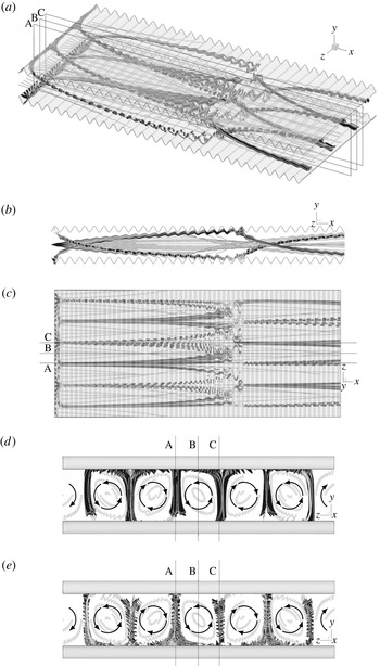
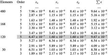
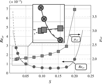
The design of compact mixing devices, such as heat exchangers, biochemical reactors, electrostatic filters, etc. is of practical importance and its improvements rely on the enhancement of mixing through creation of transverse fluid motion. Achievement of the proper mixing intensity is especially challenging for devices operating at low Reynolds numbers where flows are dominated by viscous dissipation (Bergles & Webb Reference Bergles and Webb1983). Two approaches have been utilized. The first one relies on vortex generators and is very effective but carries a large pressure drag penalty (Jacobi & Shah Reference Jacobi and Shah1995; Fiebig Reference Fiebig1995a ,Reference Fiebig b , Reference Fiebig1998). The second one relies on the promotion of the laminar–turbulent transition (Fiebig & Chen Reference Fiebig, Chen, Kaka, Bergles, Mayinger and Ync1999) and is limited to nominally subcritical flow conditions. The development of mixing enhancement is subject to important, but rarely acknowledged, constraints related to the flow-induced vibrations and the fatigue loading which needs to be avoided or, at the least, well understood in certain critical applications (Gosselin & Deardorff Reference Gosselin and Deardorff1995; International Atomic Energy Agency 2003). These constraints generate interest in developing mixing techniques which do not result in unsteady flows. Hydrodynamic instabilities which lead to the formation of secondary laminar states without triggering the transition to turbulence offer the potential to achieve this goal. Streamwise vortices represent such secondary states and, thus, identification of conduit geometries which lead to the onset of such vortices is of primary interest.
Conduits need to have a certain structural strength and one of the popular techniques to achieve this without excessive increase of the conduit mass involves use of transverse ribs. These ribs alter the flow dynamics, which could degrade the flow system performance, but their proper design could increase both the structural robustness as well as increase the desired mixing.
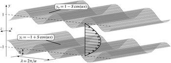
This work is focused on the analysis of the effects of transverse ribs/grooves on the character of the pressure-gradient-driven flow in a channel. The grooves have a sinusoidal shape and are placed on each wall in a manner which results in the formation of a converging–diverging channel (see figure 1). A recent literature review of flows in such geometries is provided by Rivera-Alvarez & Ordonez (Reference Rivera-Alvarez and Ordonez2013).
Channel geometry.

The interest in this problem goes back to the work of Sobey (Reference Sobey1980) and the extensive investigations of Nishimura, Ohori & Kawamura (Reference Nishimura, Ohori and Kawamura1984), Nishimura et al. (Reference Nishimura, Ohori, Kajimoto and Kawamura1985, Reference Nishimura, Murakami, Arakawa and Kawamura1990a ,Reference Nishimura, Yano, Yoshino and Kawamura b ). The problem has been looked at from two different perspectives. The first one is very applied and involves the use ribs in augmenting the heat and mass transfer (Wang & Vanka Reference Wang and Vanka1995; Wang & Chen Reference Wang and Chen2002; Bahaidarah Reference Bahaidarah2007). Lee et al. (Reference Lee, Sherrit, Tosi, Walkemeyer and Colonius2015) considers this configuration in an energy harvesting piezoelectric device. The second one is very fundamental and is focused on the onset of the oscillatory mode (Stephanoff, Sobey & Bellhouse Reference Stephanoff, Sobey and Bellhouse1980; Ralph Reference Ralph1986) and aperiodic and chaotic modes (Guzmȧn & Amon Reference Guzmȧn and Amon1994; Guzmȧn & Amon Reference Guzmȧn and Amon1996) as the relevant Reynolds number increases. We shall follow the latter approach.
It is known that the presence of grooves results in the appearance of two instability modes. The first one is the travelling wave mode (Blancher, Creff & Quere Reference Blancher, Creff and Quere1998; Floryan & Floryan Reference Floryan and Floryan2010; Cabal, Szumbarski & Floryan Reference Cabal, Szumbarski and Floryan2002; Blancher, Le Guer & El Omari Reference Blancher, Le Guer and El Omari2015) which, in the smooth channel limit, connects to the classical Tollmien–Schlichting (TS) wave. This mode is driven by shear and is responsible for the transition from stationary to oscillatory states and, eventually, to aperiodic states (Guzmȧn & Amon Reference Guzmȧn and Amon1994; Blancher et al. Reference Blancher, Creff and Quere1998). The second mode has the form of streamwise vortices and its existence has been documented experimentally (Nishimura et al. Reference Nishimura, Yano, Yoshino and Kawamura1990b ; Gschwind, Regele & Kottke Reference Gschwind, Regele and Kottke1995; Mitsudharmadi, Jamaludin & Winoto Reference Mitsudharmadi, Jamaludin, Winoto, Mastny and Perminov2012). It is attributed to the centrifugal forces associated with the groove-imposed changes of the stream direction. This mode plays the critical role in channels with a certain class of grooves (Cho, Kim & Shin Reference Cho, Kim and Shin1998; Floryan Reference Floryan2003; Floryan & Floryan Reference Floryan and Floryan2010).
The centrifugal instability is known to occur in turning shear layers. Under certain conditions, it leads to the formation of secondary flow in the form of streamwise vortices. Details of the instability have been studied for simple geometries and canonical reference flows where the streamline curvature can be easily determined and/or approximated. Rayleigh (Reference Rayleigh1917) demonstrated the inviscid character of the instability in the context of flow between concentric rotating cylinders. The fully viscous problem has been considered by Taylor (Reference Taylor1923). A similar instability has been found in curved channels by Dean (Reference Dean1928), in the case of boundary layers over concave surfaces by Görtler (Reference Görtler1941) and in the case of boundary layers over convex surfaces by Floryan (Reference Floryan1986). Analyses of flows in conduits of variable geometries are more complex as the system geometry and the resulting dynamics cannot be characterized by a single parameter. The existence of the centrifugal mode in a corrugated channel has been identified through numerical simulations by Cho et al. (Reference Cho, Kim and Shin1998) and theoretically by Cabal et al. (Reference Cabal, Szumbarski and Floryan2002), Floryan (Reference Floryan2005, Reference Floryan2003), Szumbarski (Reference Szumbarski2007). This mode connects in the smooth channel limit to a Squire mode and, thus, one may argue that the centrifugal effect amplifies (and modifies) a suitable Squire mode.
The onset of the travelling wave instability is well discussed in the literature (Blancher et al.
Reference Blancher, Creff and Quere1998; Cho et al.
Reference Cho, Kim and Shin1998; Floryan & Floryan Reference Floryan and Floryan2010; Rivera-Alvarez & Ordonez Reference Rivera-Alvarez and Ordonez2013; Blancher et al.
Reference Blancher, Le Guer and El Omari2015) and its dependence on the geometric parameters is known for small-amplitude grooves (Floryan & Floryan Reference Floryan and Floryan2010) and for selected large-amplitude grooves (Cho et al.
Reference Cho, Kim and Shin1998). The centrifugal instability has been studied less frequently, primarily due to its three-dimensional character. Cho et al. (Reference Cho, Kim and Shin1998) investigated both modes but only for a single corrugation wavelength
 $\unicode[STIX]{x1D706}=3$
and with amplitudes large enough for the recirculation zone to form within troughs. Floryan (Reference Floryan2003) considered a full range of corrugation wavelengths, but limited the investigation to small amplitudes, suggesting that for larger amplitudes, the centrifugal effect is weakened by the growth of the recirculation zone (Oviedo-Tolentino et al.
Reference Oviedo-Tolentino, Romero-Mėndez, Hernȧndez-Guerrero and Girȯn-Palomares2008; Floryan & Floryan Reference Floryan and Floryan2010). In a later paper by Floryan & Floryan (Reference Floryan and Floryan2010) attention was given to the onset of the travelling wave instability. It was shown that this instability is dominant for small amplitudes but is quickly overcome by the centrifugal instability as soon as the corrugation amplitude is increased. The conclusions are similar to those of Cho et al. (Reference Cho, Kim and Shin1998) who studied just one corrugation wavelength and showed that, while moderate corrugation amplitudes result in the centrifugal instability being dominant, their increase results in a larger separation zone which brings back the travelling wave instability.
The main focus of this work is mapping of the dynamics of the flow in a converging–diverging channel (see figure 1) with the groove wavenumber varied from
 $\unicode[STIX]{x1D6FC}=10$
(short-wavelength grooves) to
 $\unicode[STIX]{x1D6FC}=0.5$
(long-wavelength grooves) which covers the full range of wavelengths of practical importance. The analysis is performed under the assumption of a fully developed and periodic flow regime. It is limited to moderate groove amplitudes, i.e.
 $S<0.2$
, and relies on direct numerical simulation (DNS) based on the spectral finite-element method in the
 $(x,y)$
-plane combined with the Fourier decomposition in the spanwise direction, as implemented in NEKTAR
 $++$
(Cantwell et al.
Reference Cantwell, Moxey, Comerford, Bolis, Rocco, Mengaldo, Grazia, Yakovlev, Lombard and Ekelschot2015; Bolis et al.
Reference Bolis, Cantwell, Kirby and Sherwin2014). The analysis is divided into two steps, with the first one focused on the two-dimensional dynamics and presenting flow properties up to the formation of secondary states. Two issues are of particular interest, i.e. drag penalty associated with the grooves and onset of separation, particularly the unsteady separation. The second step involves analysis of three-dimensional dynamics and identification of conditions when such dynamics precedes the two-dimensional dynamics. Determination of conditions leading to the onset of streamwise vortices is of particular interest. The drag penalty associated with the formation of such vortices, as well as the identification of geometries where such vortices can be created without interference from the travelling wave instability, are of interest.
This paper is organized as follows. Section 2 describes the two-dimensional flow model. In particular, § 2.1 presents problem formulation, § 2.2 discusses numerical method used and § 2.3 discusses various features of the two-dimensional flow field. Section 3 describes three-dimensional flow dynamics. In particular, § 3.1 gives problem formulation, § 3.2 describes numerical technique and § 3.3 discusses the key feature of the three-dimensional flow dynamics. Section 4 describes saturation states resulting from the instability-induced flow three-dimensionalization including topologies of such states. Section 5 provides a short summary of the main conclusions.
2 Two-dimensional flow dynamics
Consider flow of an incompressible Newtonian fluid through a converging–diverging channel as displayed in figure 1. The channel extends to
 $\pm \infty$
in the streamwise
 $x$
- and spanwise
 $z$
-directions and the flow is driven in the positive
 $x$
-direction by a constant pressure gradient. A typical channel section has wavelength
 $\unicode[STIX]{x1D706}=2\unicode[STIX]{x03C0}/\unicode[STIX]{x1D6FC}$
where
 $\unicode[STIX]{x1D6FC}$
stands for the groove wavenumber, the corrugation has amplitude
 $S$
, the walls are located at
 $$\begin{eqnarray}\displaystyle \left.\begin{array}{@{}c@{}}\displaystyle y=y_{u}=1-S\cos (\unicode[STIX]{x1D6FC}x),\\ \displaystyle y=y_{l}=-1+S\cos (\unicode[STIX]{x1D6FC}x)\end{array}\right\} & & \displaystyle\end{eqnarray}$$
and all geometric quantities have been scaled with the half-width
 $h$
of the reference smooth channel (
 $S=0$
). While the channel geometry is two-dimensional, the flow in general does not need to be two-dimensional. We shall start the analysis by focusing on the two-dimensional dynamics and return to the question of three-dimensionality in § 3.
2.1 Problem formulation
Flow evolution is described by the Navier–Stokes and continuity equation of the form
 $$\begin{eqnarray}\displaystyle \left.\begin{array}{@{}c@{}}\displaystyle \unicode[STIX]{x1D735}\boldsymbol{\cdot }\boldsymbol{u}=0,\\ \displaystyle \frac{\unicode[STIX]{x2202}\boldsymbol{u}}{\unicode[STIX]{x2202}t}+\boldsymbol{u}\boldsymbol{\cdot }\unicode[STIX]{x1D735}\boldsymbol{u}=-\unicode[STIX]{x1D735}p+\frac{1}{Re}\unicode[STIX]{x1D6FB}^{2}\boldsymbol{u},\end{array}\right\} & & \displaystyle\end{eqnarray}$$
where
 $\boldsymbol{u}=[u,v,w]^{\text{T}}$
is the velocity vector,
 $p$
is the pressure, the maximum of the streamwise velocity in the reference smooth channel,
 $U_{s}$
, has been used as the velocity scale,
 $\unicode[STIX]{x1D71A}U_{s}^{2}$
has been used as the pressure scale with
 $\unicode[STIX]{x1D71A}$
denoting density,
 $h/U_{s}$
plays the role of the time scale and
 $Re=(U_{s}h)/\unicode[STIX]{x1D708}$
stands for the Reynolds number with
 $\unicode[STIX]{x1D708}$
being the kinematic viscosity. The boundary conditions at the walls have the form of
 $$\begin{eqnarray}\displaystyle \boldsymbol{u}=0\quad \text{at }\left\{\begin{array}{@{}l@{}}y=y_{u},\quad \\ y=y_{l}.\quad \end{array}\right. & & \displaystyle\end{eqnarray}$$
We shall impose periodicity conditions in the
 $x$
-direction as a periodic geometry is expected to create periodic flow modulations. In general, periodicities of geometry and flow modulations do not need to be identical and this fact needs to be accounted for while selecting the computational domain. Since this domain needs to be finite, direct analysis of incommensurable states is not possible but the potential existence of such states could be inferred by using limiting processes and analytical arguments.
The reference flow has the form of plane Poiseuille flow confined between flat rigid walls at
 $y=\pm 1$
. The fluid motion has velocity
 $\boldsymbol{u}$
, pressure
 $p$
and flow rate
 $Q_{r}$
of the form:
 $$\begin{eqnarray}\displaystyle \left.\begin{array}{@{}c@{}}\displaystyle \boldsymbol{u}=[1-y^{2},0],\\ \displaystyle p=-\frac{2x}{Re},\\ \displaystyle Q_{r}=\frac{4}{3}.\end{array}\right\} & & \displaystyle\end{eqnarray}$$
It is assumed that while the channel morphs into the converging–diverging form, the pressure gradient driving the flow remains the same, resulting in changes of the flow rate. This process corresponds to the imposition of the pressure-gradient constraint of the form
 $$\begin{eqnarray}\displaystyle \left.\frac{\unicode[STIX]{x2202}p}{\unicode[STIX]{x2202}x}\right|_{mean}=\frac{-2}{Re}, & & \displaystyle\end{eqnarray}$$
with the resulting flow rate determined a posteriori. This means that the effective Reynolds number is a function of the groove geometry.
Problem (2.2)–(2.5) is solved numerically using an incompressible Navier–Stokes solver available in the NEKTAR
 $++$
software package (Cantwell et al.
Reference Cantwell, Moxey, Comerford, Bolis, Rocco, Mengaldo, Grazia, Yakovlev, Lombard and Ekelschot2015; Bolis et al.
Reference Bolis, Cantwell, Kirby and Sherwin2014). Spatial discretization is based on the spectral element method. Simulations have been carried out using a regular, structured quadrilateral mesh combined with fifth-order polynomials. The mesh has been generated using the GMSH package (Geuzaine & Remacle Reference Geuzaine and Remacle2009). The computational box extends over an integer number of corrugation wavelengths in the streamwise direction. Selection of the number of wavelengths is dictated by the flow physics. The flow is assumed to be periodic in the streamwise and spanwise directions. The temporal discretization uses the second-order velocity-correction scheme (Guermond & Shen Reference Guermond and Shen2003). The kinetic energy evolution criterion is used to test the existence of steady states. Average kinetic energy per unit area over the computational domain
 $\unicode[STIX]{x1D6FA}$
is defined as
 $$\begin{eqnarray}\displaystyle E_{k}(t)=\frac{1}{\unicode[STIX]{x1D6FA}}\int _{\unicode[STIX]{x1D6FA}}\frac{1}{2}\Vert \boldsymbol{u}(t)\Vert ^{2}\,\text{d}\unicode[STIX]{x1D6FA} & & \displaystyle\end{eqnarray}$$
and the simulations are assumed to reach a steady state when the energy change
 $\unicode[STIX]{x1D6FF}E_{r}$
defined as:
 $$\begin{eqnarray}\displaystyle \unicode[STIX]{x1D6FF}E_{r}=\frac{\underset{T_{f}-T_{l}\leqslant t\leqslant T_{f}}{\max }E_{k}(t)-\underset{T_{f}-T_{l}\leqslant t\leqslant T_{f}}{\min }E_{k}(t)}{\underset{T_{f}-T_{l}\leqslant t\leqslant T_{f}}{\max }E_{k}(t)} & & \displaystyle\end{eqnarray}$$
reaches a certain, predefined threshold in a suitably selected time interval. Here,
 $T_{f}$
represents the simulation final time and
 $T_{l}$
stands for the time interval over which the stationarity test is conducted. In the current study we use
 $T_{l}=10^{4}$
and
 $\unicode[STIX]{x1D6FF}E_{r}=10^{-6}$
. Verification of the spatial accuracy and testing required for the grid selection have been carried out using a computational box containing one corrugation wavelength with details given in appendix A. If the computational box contains several corrugation wavelengths, the same grid is used in each section corresponding to one corrugation wavelength.
2.2 Description of two-dimensional states
2.2.1 Long-wavelength corrugation
The stationary state in the limit of long corrugation wavelength (
 $\unicode[STIX]{x1D6FC}\rightarrow 0$
) can be determined analytically, following Mohammadi & Floryan (Reference Mohammadi and Floryan2012). The first step is to regularize the flow domain using a transformation of the form:
 $$\begin{eqnarray}\displaystyle \left.\begin{array}{@{}c@{}}\displaystyle \unicode[STIX]{x1D709}=\unicode[STIX]{x1D6FC}x,\\ \displaystyle \unicode[STIX]{x1D702}=\frac{y-1+S\cos (\unicode[STIX]{x1D6FC}x)}{1-S\cos (\unicode[STIX]{x1D6FC}x)}+1\end{array}\right\} & & \displaystyle\end{eqnarray}$$
leading to the field equations of the form:
 $$\begin{eqnarray}\displaystyle \left.\begin{array}{@{}c@{}}\displaystyle \unicode[STIX]{x1D6FC}\frac{\unicode[STIX]{x2202}u}{\unicode[STIX]{x2202}\unicode[STIX]{x1D709}}+F_{11}\frac{\unicode[STIX]{x2202}u}{\unicode[STIX]{x2202}\unicode[STIX]{x1D702}}+F_{12}\frac{\unicode[STIX]{x2202}v}{\unicode[STIX]{x2202}\unicode[STIX]{x1D702}}=0,\\ \displaystyle -\frac{\unicode[STIX]{x2202}^{2}u}{\unicode[STIX]{x2202}\unicode[STIX]{x1D702}^{2}}-F_{1}\frac{\unicode[STIX]{x2202}u}{\unicode[STIX]{x2202}\unicode[STIX]{x1D702}}+F_{2}u\frac{\unicode[STIX]{x2202}u}{\unicode[STIX]{x2202}\unicode[STIX]{x1D702}}+F_{3}v\frac{\unicode[STIX]{x2202}u}{\unicode[STIX]{x2202}\unicode[STIX]{x1D702}}-F_{4}\frac{\unicode[STIX]{x2202}^{2}u}{\unicode[STIX]{x2202}\unicode[STIX]{x1D709}\unicode[STIX]{x2202}\unicode[STIX]{x1D702}}-F_{5}\frac{\unicode[STIX]{x2202}^{2}u}{\unicode[STIX]{x2202}\unicode[STIX]{x1D709}^{2}}+F_{6}u\frac{\unicode[STIX]{x2202}u}{\unicode[STIX]{x2202}\unicode[STIX]{x1D709}}\\ \displaystyle \hspace{-128.39996pt}+\,F_{6}\frac{\unicode[STIX]{x2202}P}{\unicode[STIX]{x2202}\unicode[STIX]{x1D709}}+F_{2}\frac{\unicode[STIX]{x2202}p}{\unicode[STIX]{x2202}\unicode[STIX]{x1D702}}=0,\\ \displaystyle -\frac{\unicode[STIX]{x2202}^{2}v}{\unicode[STIX]{x2202}\unicode[STIX]{x1D702}^{2}}-F_{1}\frac{\unicode[STIX]{x2202}v}{\unicode[STIX]{x2202}\unicode[STIX]{x1D702}}+F_{2}u\frac{\unicode[STIX]{x2202}v}{\unicode[STIX]{x2202}\unicode[STIX]{x1D702}}+F_{3}v\frac{\unicode[STIX]{x2202}v}{\unicode[STIX]{x2202}\unicode[STIX]{x1D702}}-F_{4}\frac{\unicode[STIX]{x2202}^{2}v}{\unicode[STIX]{x2202}\unicode[STIX]{x1D709}\unicode[STIX]{x2202}\unicode[STIX]{x1D702}}-F_{5}\frac{\unicode[STIX]{x2202}^{2}v}{\unicode[STIX]{x2202}\unicode[STIX]{x1D709}^{2}}+F_{6}u\frac{\unicode[STIX]{x2202}v}{\unicode[STIX]{x2202}\unicode[STIX]{x1D709}}+F_{3}\frac{\unicode[STIX]{x2202}p}{\unicode[STIX]{x2202}\unicode[STIX]{x1D702}}=0\end{array}\right\}\quad & & \displaystyle\end{eqnarray}$$
subject to boundary conditions:
 $$\begin{eqnarray}\displaystyle \boldsymbol{u}=0\quad \text{at }\unicode[STIX]{x1D702}=\pm 1. & & \displaystyle\end{eqnarray}$$
The coefficients in the above equations are defined as:
 $$\begin{eqnarray}\displaystyle \left.\begin{array}{@{}c@{}}\displaystyle F_{1}=-\unicode[STIX]{x1D6FC}^{2}\frac{2F_{9}F_{13}-F_{8}F_{10}}{F_{7}},\quad F_{2}=Re\frac{F_{4}}{2\unicode[STIX]{x1D6FC}},\quad F_{3}=2Re\frac{F_{8}}{F_{7}},\\ \displaystyle F_{4}=2\unicode[STIX]{x1D6FC}^{2}\frac{F_{9}F_{8}}{F_{7}},\quad F_{5}=\unicode[STIX]{x1D6FC}^{2}\frac{F_{8}^{2}}{F_{7}},\quad F_{6}=Re\frac{F_{5}}{\unicode[STIX]{x1D6FC}},\\ \displaystyle F_{7}=4+\unicode[STIX]{x1D6FC}^{2}F_{9}^{2},\quad F_{8}=2-2S\cos (\unicode[STIX]{x1D709}),\quad F_{9}=-2S\unicode[STIX]{x1D702}\sin (\unicode[STIX]{x1D709}),\\ \displaystyle F_{10}=-2S\unicode[STIX]{x1D702}\cos (\unicode[STIX]{x1D709}),\quad F_{11}=\unicode[STIX]{x1D6FC}\frac{F_{9}}{F_{8}},\quad F_{12}=\frac{2}{F_{8}},\\ \displaystyle F_{13}=2S\sin (\unicode[STIX]{x1D709}).\end{array}\right\} & & \displaystyle\end{eqnarray}$$
The solution to (2.9) is represented in terms of power expansions of the form:
 $$\begin{eqnarray}\displaystyle \left.\begin{array}{@{}c@{}}\displaystyle u=u_{0}+\unicode[STIX]{x1D6FC}u_{1}+O(\unicode[STIX]{x1D6FC}^{2}),\\ \displaystyle v=v_{0}+\unicode[STIX]{x1D6FC}v_{1}+O(\unicode[STIX]{x1D6FC}^{2}),\\ \displaystyle p=\unicode[STIX]{x1D6FC}^{-1}p_{-1}+p_{0}+O(\unicode[STIX]{x1D6FC}).\end{array}\right\} & & \displaystyle\end{eqnarray}$$
Substituting (2.12) into (2.9) and retaining the two leading-order terms leads to a sequence of problems with the leading-order system of the form:
 $$\begin{eqnarray}\displaystyle \left.\begin{array}{@{}c@{}}\displaystyle -\frac{\unicode[STIX]{x2202}^{2}u_{0}}{\unicode[STIX]{x2202}\unicode[STIX]{x1D702}^{2}}+\frac{Re{F_{8}}^{2}}{4}\frac{\unicode[STIX]{x2202}p_{-1}}{\unicode[STIX]{x2202}\unicode[STIX]{x1D709}}=0,\\ \displaystyle \frac{\unicode[STIX]{x2202}p_{-1}}{\unicode[STIX]{x2202}\unicode[STIX]{x1D702}}=0,\\ \displaystyle \frac{\unicode[STIX]{x2202}v_{0}}{\unicode[STIX]{x2202}\unicode[STIX]{x1D702}}=0.\end{array}\right\} & & \displaystyle\end{eqnarray}$$
The next-order system has the form:
 $$\begin{eqnarray}\displaystyle \left.\begin{array}{@{}c@{}}\displaystyle -\frac{\unicode[STIX]{x2202}^{2}u_{1}}{\unicode[STIX]{x2202}\unicode[STIX]{x1D702}^{2}}+\frac{ReF_{9}F_{8}}{4}u_{0}\frac{\unicode[STIX]{x2202}u_{0}}{\unicode[STIX]{x2202}\unicode[STIX]{x1D702}}+\frac{ReF_{8}}{2}v_{1}\frac{\unicode[STIX]{x2202}u_{0}}{\unicode[STIX]{x2202}\unicode[STIX]{x1D702}}+\frac{ReF_{8}^{2}}{4}u_{0}\frac{\unicode[STIX]{x2202}u_{0}}{\unicode[STIX]{x2202}\unicode[STIX]{x1D709}}+\frac{ReF_{8}^{2}}{4}\frac{p_{0}}{\unicode[STIX]{x2202}\unicode[STIX]{x1D709}}=0,\\ \displaystyle \frac{\unicode[STIX]{x2202}p_{0}}{\unicode[STIX]{x2202}\unicode[STIX]{x1D702}}=0,\\ \displaystyle \frac{\unicode[STIX]{x2202}u_{0}}{\unicode[STIX]{x2202}\unicode[STIX]{x1D709}}+\frac{F_{9}}{F_{8}}\frac{\unicode[STIX]{x2202}u_{0}}{\unicode[STIX]{x2202}\unicode[STIX]{x1D702}}+\frac{2}{F_{8}}\frac{\unicode[STIX]{x2202}v_{1}}{\unicode[STIX]{x2202}\unicode[STIX]{x1D702}}=0.\end{array}\right\} & & \displaystyle\end{eqnarray}$$
The solution of (2.13) is:
 $$\begin{eqnarray}\displaystyle \left.\begin{array}{@{}c@{}}\displaystyle u_{0}=2M\frac{1-\unicode[STIX]{x1D702}^{2}}{F_{8}},\\ \displaystyle v_{0}=0,\\ \displaystyle p_{-1}=-\frac{H(2+S^{2})}{\sqrt{(1-S^{2})^{5}}}\arctan \left[\frac{\sqrt{1-S}}{\sqrt{1+S}}\tan \left(\frac{\unicode[STIX]{x1D709}}{2}\right)-\frac{\unicode[STIX]{x03C0}}{2}\right]\\ \displaystyle \hspace{31.20007pt}-\,\frac{0.5HS\sin (\unicode[STIX]{x1D709}-\unicode[STIX]{x03C0})[-3S\cos (\unicode[STIX]{x1D709}-\unicode[STIX]{x03C0})+S^{2}-4]}{(1-S^{2})^{2}[1+S\cos (\unicode[STIX]{x1D709}-\unicode[STIX]{x03C0})]^{2}}\\ \displaystyle \hspace{-79.20007pt}-\,\frac{H\unicode[STIX]{x03C0}(2+S^{2})}{\sqrt{(1-S^{2})^{5}}}\left\lfloor \frac{\unicode[STIX]{x1D709}}{2\unicode[STIX]{x03C0}}\right\rfloor \end{array}\right\} & & \displaystyle\end{eqnarray}$$
and the solution of (2.14) is:
 $$\begin{eqnarray}\displaystyle \left.\begin{array}{@{}c@{}}\displaystyle u_{1}=ReM^{2}\frac{F_{13}}{F_{8}}\left(-\frac{1}{30}\unicode[STIX]{x1D702}^{6}+\frac{1}{6}\unicode[STIX]{x1D702}^{4}-\frac{11}{70}\unicode[STIX]{x1D702}^{2}+\frac{5}{210}\right),\\ \displaystyle v_{1}=\frac{M}{F_{8}}[-S\sin (\unicode[STIX]{x1D709})(\unicode[STIX]{x1D702}^{3}+\unicode[STIX]{x1D702}^{2}-\unicode[STIX]{x1D702}-1)+S\sin (\unicode[STIX]{x1D709})(-\unicode[STIX]{x1D702}^{3}+\unicode[STIX]{x1D702}^{2}+\unicode[STIX]{x1D702}-1)],\\ \displaystyle p_{0}=-\frac{48M^{2}}{35F_{8}^{2}}+c_{0},\end{array}\right\} & & \displaystyle\end{eqnarray}$$
where
 $M=\sqrt{(1-S^{2})^{5}}/(1+S^{2}/2)$
,
 $H=2M/Re$
,
 $c_{0}=12M/(35(1-S)^{2})-(p_{-1}(0))/\unicode[STIX]{x1D6FC}$
is the pressure normalization such that
 $p=0$
at
 $\unicode[STIX]{x1D709}=0$
. The last operator used in the expression for
 $p_{-1}$
is the floor function
 $\lfloor \cdot \rfloor$
which is added to remove spurious discontinuities associated with the inverse tangent function (Jeffrey & Rich Reference Jeffrey and Rich1994; Mohammadi & Floryan Reference Mohammadi and Floryan2012). The flow rate calculated using the approximate solution (2.15)–(2.16), is:
 $$\begin{eqnarray}\displaystyle Q=\frac{4}{3}\frac{\sqrt{(1-S^{2})^{5}}}{1+\displaystyle \frac{S^{2}}{2}}+O(\unicode[STIX]{x1D6FC}^{2}), & & \displaystyle\end{eqnarray}$$
i.e. it is not equal to the reference value of
 $Q_{r}=4/3$
for
 $\unicode[STIX]{x1D6FC}\rightarrow 0$
, unless
 $S=0$
. One can define a Reynolds number based on the flow rate in the form of
 $$\begin{eqnarray}\displaystyle Re_{av}=\frac{Q}{2\unicode[STIX]{x1D708}} & & \displaystyle\end{eqnarray}$$
as it provides a useful assessment tool for the state of the flow. The reference value of
 $Re_{av}$
for the smooth channel relates to
 $Re$
defined in § 2.1 as:
 $$\begin{eqnarray}\displaystyle \frac{Re_{av}}{Re}=\frac{6}{4}. & & \displaystyle\end{eqnarray}$$
2.2.2 Corrugations with wavelength
 $O(1)$

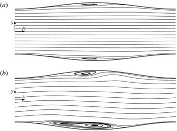
The analysis of flows in channels with a long-wavelength convergence–divergence discussed in the previous section demonstrates the existence of stationary states and the absence of flow separation. Reduction of the wavelength leads to the onset of separation, as illustrated in figure 2 for
 $\unicode[STIX]{x1D6FC}=1$
. This separation occurs in the expanding section of the channel, and is stationary and symmetric in the
 $y$
-direction when
 $S$
is small enough (see figure 2
a). An increase of
 $S$
while keeping the same
 $Re$
results in a transition to an oscillatory separation which does not preserve the symmetry (see figure 2
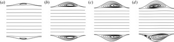
b). Further reduction of the wavelength leads to an analogous sequence of changes in the flow topology, as illustrated in figure 3 for
 $\unicode[STIX]{x1D6FC}=3$
. Steady separation occurs for
 $S=0.075$
(see figure 3
a), the size of the separation zone increases when measured in terms of the fraction of the trough height as
 $S$
increases (see figure 3
b), it almost completely fills in the trough for
 $S=0.2$
, pushing the stream away from the walls (see figure 3
c), and it becomes oscillatory for
 $S=0.225$
(see figure 3
d). At
 $\unicode[STIX]{x1D6FC}=8$
(not shown) no oscillatory separation has been found in the range of
 $S$
and
 $Re$
considered in this study.
Streamlines of the stationary (
 $S=0.125$
,
 $\unicode[STIX]{x1D6EF}=5.48\times 10^{-6}$
) (a) and a snapshot of an oscillatory (
 $S=0.150$
,
 $\unicode[STIX]{x1D6EF}=1.15\times 10^{-1}$
) (b) velocity field.
 $\unicode[STIX]{x1D6FC}=1$
,
 $Re=1500$
. Computational boxes containing one corrugation wavelength have been used to produce these results.

Development of the recirculation zone for
 $\unicode[STIX]{x1D6FC}=3$
,
 $Re=2300$
, at different corrugation amplitudes: (a)
 $S=0.075$
, (b)
 $S=0.150$
, (c)
 $S=0.2$
and (d)
 $S=0.225$
(a snapshot of an oscillatory solution). Computational boxes containing one corrugation wavelength have been used to produce these results.

The above discussion demonstrates the existence of three states, i.e. the stationary states with no separation, the stationary states with symmetric separation and the oscillatory states with non-symmetric separation, and leads to the question of the determination of conditions leading to the appearance of these states. Steady separation can be easily detected through an analysis of the flow field. Identification of the onset of the oscillatory separation is more complex as the numerical solution relies on time simulations and stationary states are detected by examining the time history of the relevant flow properties, e.g. kinetic energy, discussed in § 2.1. The convergence of the numerical process is always oscillatory and, thus, one needs to develop a reliable criterion for separation of the purely numerical oscillations from the physical oscillations, especially at the onset when the physical oscillations have very small amplitudes. Since it has been observed by Cho et al. (Reference Cho, Kim and Shin1998) that stationary flows through symmetric channels exhibit symmetry with respect to the centreline (see figures 2
a, 3
a,b,c;
 $u$
is symmetric,
 $v$
is anti-symmetric,
 $p$
is symmetric) and transition to the oscillatory flow happens through breaking of this symmetry, we use change in the flow symmetry as a criterion for identification of the onset of flow unsteadiness. Accordingly, we define the symmetricity parameter
 $\unicode[STIX]{x1D6EF}$
as:
 $$\begin{eqnarray}\displaystyle \unicode[STIX]{x1D6EF}=\frac{1}{N}\mathop{\sum }_{1}^{N}\int _{0}^{y_{u}(x_{n})}(|u(y)-u(-y)|+|v(y)+v(-y)|+|p(y)-p(-y)|)\,\text{d}y & & \displaystyle\end{eqnarray}$$
over a snap shot of the flow field where
 $N$
is the number of sample points over one corrugation wavelength and
 $y_{u}(x_{n})$
denotes point at the upper wall at
 $x_{n}$
.
 $N=9$
sample points have been used in this work with all points spaced evenly in the
 $x$
-direction from
 $x=0.1\unicode[STIX]{x1D706}$
to
 $x=0.9\unicode[STIX]{x1D706}$
.
Variations of the size of the separation zone measured at the widest channel opening as a function of
 $Re$
for stationary flows.

 $S=0.025$
,

 $S=0.05$
,

 $S=0.075$
,

 $S=0.1$
,

 $S=0.125$
,

 $S=0.15$
,

 $S=0.175$
,

 $S=0.2$
. Computational boxes containing one corrugation wavelength have been used to produce these results.

We shall now discuss properties of stationary flows. Here we define such flows as flows with
 $\unicode[STIX]{x1D6EF}<10^{-3}$
. We shall describe a more precise stationarity measure in the next section. We shall limit our interest to
 $S<0.2$
and
 $Re<3500$
. The reasons for selecting this range of parameters will become more obvious as we progress through the discussion. Data displayed in figure 4 provide information about variations of the size of the separation zone as a function of the channel geometry and flow conditions. We shall use the height of the separation bubble
 $H$
at the widest channel opening as a measure of the size of separation. For long enough corrugations (figure 4
a), it is possible to avoid separation for a given
 $S$
if
 $Re$
is small enough;
 $Re$
needs to reach a certain minimum threshold before separation can take place. An increase of
 $S$
reduces this threshold. Once separation appears, an increase of
 $Re$
results in an increase of
 $H$
with
 $H/S=2$
being the upper limit corresponding to the bubble completely filling in the trough. This increase is very rapid for large
 $S$
(see
 $S=0.2$
in figure 4
a for
 $\unicode[STIX]{x1D6FC}=2$
) and very gradual for smaller
 $S$
(see
 $S=0.025$
,
 $\unicode[STIX]{x1D6FC}=2$
in figure 4
a). Reduction of the groove wavelength results in a qualitatively similar process with the bubble size increasing more rapidly than for
 $\unicode[STIX]{x1D6FC}=2$
(compare results in figure 4
b for
 $\unicode[STIX]{x1D6FC}=5$
with results for
 $\unicode[STIX]{x1D6FC}=2$
in figure 4
a). Further reduction of the groove wavelength continues this process (see results for
 $\unicode[STIX]{x1D6FC}=8$
in figure 4
c). It can be seen that in the case of grooves with shorter wavelengths, an increase of
 $S$
results in the trough being filled very rapidly by the separation bubble (see figure 4
b,c) resulting in the stream being pushed away from the walls.
The presence of grooves affects the flow topology, as discussed above, and results in an increase of the flow resistance. As the pressure gradient is kept constant, increase of the resistance manifests itself through the reduction of the flow rate
 $Q$
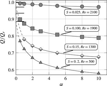
. Figure 5 illustrates the character of these variations as a function of the geometry and the flow conditions. Reduction of
 $Q$
is rather small and insensitive to variations of
 $Re$
for the long-wavelength, small-amplitude grooves. These variations become much bigger and very sensitive to
 $Re$
for larger amplitudes (see results figure 5
a for
 $\unicode[STIX]{x1D6FC}=0.5$
). The reduction of the groove wavelength to
 $\unicode[STIX]{x1D6FC}=3$
(figure 5
b) and
 $\unicode[STIX]{x1D6FC}=8$
(figure 5
c) results in a significant reduction of
 $Q$
as the separation bubbles fill in a significant portion of the cross-sectional flow area. At the same time the flow losses become insensitive to variations of
 $Re$
and
 $\unicode[STIX]{x1D6FC}$
(compare figure 5
b,c). The latter fact is well illustrated in figure 6 displaying variations of
 $Q$
as a function of
 $\unicode[STIX]{x1D6FC}$
. The relative sensitivity of these losses for small
 $\unicode[STIX]{x1D6FC}$
and large
 $S$
and their relative insensitivity for large
 $\unicode[STIX]{x1D6FC}$
and small
 $S$
are well illustrated.
Variations of the flow rate
 $Q$
as a function of
 $Re$
for stationary flows.

 $S=0.025$
,

 $S=0.05$
,

 $S=0.075$
,

 $S=0.1$
,

 $S=0.125$
,

 $S=0.15$
,

 $S=0.175$
,

 $S=0.2$
. Computational boxes containing one corrugation wavelength have been used to produce these results.

Variation of the flow rate
 $Q$
as a function of the corrugation wavenumber
 $\unicode[STIX]{x1D6FC}$
for stationary flows. Thick lines identify limits for
 $\unicode[STIX]{x1D6FC}\rightarrow 0$
. Computational boxes containing one corrugation wavelength have been used to produce these results.

The reduction of
 $Q$
leads to the slowing down of the flow and reduction of the effective Reynolds number. This reduction is marginal for small
 $\unicode[STIX]{x1D6FC}$
(see figure 7
a) but becomes more and more significant as
 $\unicode[STIX]{x1D6FC}$
increases (see figure 7
b,c). These changes in the effective Reynolds number need to be accounted for in the discussion of stability properties of the flow.
Variations of the flow rate based Reynolds number
 $Re_{av}$
as a function of
 $Re$
for stationary flows.

 $S=0.025$
,

 $S=0.05$
,

 $S=0.075$
,

 $S=0.1$
,

 $S=0.125$
,

 $S=0.15$
,

 $S=0.175$
,

 $S=0.2$
. The dashed line corresponds to the smooth channel where
 $Re_{av}=6/4Re$
. Computational boxes containing one corrugation wavelength have been used to produce these results.

2.3 Transition to oscillatory flow
Figure 8 illustrates variations of
 $\unicode[STIX]{x1D6EF}$
as a function of
 $Re$
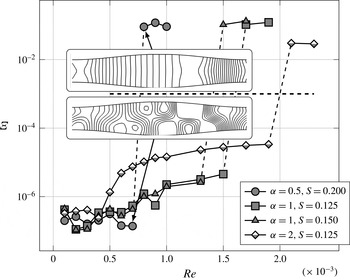
, for a few illustrative geometries. The investigations were performed using computational boxes containing one corrugation wavelength. It is quite clear that there exists a critical value of
 $Re$
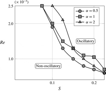
which separates two distinctive states, one being stationary and the other being oscillatory. Variations of the critical
 $Re$
as a function of
 $\unicode[STIX]{x1D6FC}$
and
 $S$
illustrated in figure 9 suggest that oscillatory states occur for smaller
 $Re$
and
 $S$
for grooves with smaller
 $\unicode[STIX]{x1D6FC}$
. Crossing of lines for
 $\unicode[STIX]{x1D6FC}=1$
and
 $\unicode[STIX]{x1D6FC}=2$
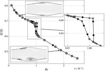
suggests otherwise, but this is an artefact of the method used in this analysis related to the size of the computational box, as explained later in this section. The consequences of transition to an oscillatory state are illustrated in figure 10 displaying variations of the flow rate
 $Q$
as a function of
 $Re$
. A rapid drop in
 $Q$
accompanies such a transition. A hysteresis in the change of
 $Q$
has been observed depending on whether
 $Re$
is increasing and the system transits from a stationary to the oscillatory state, or
 $Re$
is decreasing and the system transits from the oscillatory to the stationary state.
Variations of the symmetricity parameter (see (2.20) for definition) as a function of
 $Re$
. Flows with
 $\unicode[STIX]{x1D6EF}>10^{-3}$
are considered to be non-stationary. Internal boxes display instantaneous pressure fields at the jump points. Computational boxes containing one corrugation wavelength have been used to produce these results.

Borders between the stationary and oscillatory states in the
 $(Re,S)$
-plane identified using
 $\unicode[STIX]{x1D6EF}=10^{-3}$
criterion. Locations of the borders have been determined approximately due to the subcritical character of transition between both states. The intersection of curves for
 $\unicode[STIX]{x1D6FC}=1$
and
 $\unicode[STIX]{x1D6FC}=2$
results from the change of the wavenumber
 $\unicode[STIX]{x1D6FF}$
of the most unstable wave as a function of the amplitude
 $S$
. Computational boxes containing one corrugation wavelength have been used to produce these results.

Variations of the flow rate
 $Q$
as a function of
 $Re$
for
 $\unicode[STIX]{x1D6FC}=1$
and
 $S=0.2$
.
 $\unicode[STIX]{x1D6EF}=10^{-3}$
criterion has been used to distinguish between the stationary and oscillatory states. Computational boxes containing one corrugation wavelength have been used to produce these results.

The features of transition between the stationary and oscillatory states described above suggest that the mechanics of the process can be described using stability techniques and the onset of the oscillatory state represents a subcritical Hopf bifurcation. It has been argued that the instability has the form of a two-dimensional travelling wave analogous to the TS waves (Ghaddar et al. Reference Ghaddar, Korczak, Mikic and Patera1986; Guzmȧn & Amon Reference Guzmȧn and Amon1994; Cho et al. Reference Cho, Kim and Shin1998) arising at Reynolds numbers significantly smaller than for the flow in a smooth channel.
In order to determine the critical conditions leading to transition from stationary to oscillatory states, we represent the total flow quantities as a superposition of the stationary flow, described in § 2.2.2 and a small disturbance, i.e.
 $$\begin{eqnarray}\displaystyle \left.\begin{array}{@{}c@{}}\displaystyle \boldsymbol{U}_{T}(x,y,z,t)=\boldsymbol{U}(x,y)+\boldsymbol{u}_{p}(x,y,z,t),\\ \displaystyle P_{T}(x,y,z,t)=P(x,y)+p_{p}(x,y,z,t),\end{array}\right\} & & \displaystyle\end{eqnarray}$$
where the subscripts
 $T$
and
 $p$
refer to the total flow quantities and small disturbances, respectively. Substitution of (2.21) into the field equation (2.2) and linearisation lead to the disturbance equation of the form
 $$\begin{eqnarray}\displaystyle \left.\begin{array}{@{}c@{}}\displaystyle \unicode[STIX]{x1D735}\boldsymbol{\cdot }\boldsymbol{u}_{\boldsymbol{p}}=0,\\ \displaystyle \frac{\unicode[STIX]{x2202}u_{p}}{\unicode[STIX]{x2202}t}+\boldsymbol{u}_{\boldsymbol{p}}\boldsymbol{\cdot }\unicode[STIX]{x1D735}\boldsymbol{U}+\boldsymbol{U}\boldsymbol{\cdot }\unicode[STIX]{x1D735}\boldsymbol{u}_{\boldsymbol{p}}=-\frac{1}{\unicode[STIX]{x1D71A}}\unicode[STIX]{x1D735}p_{p}+\frac{1}{Re}\unicode[STIX]{x1D6FB}^{2}\boldsymbol{u}_{\boldsymbol{ p}}.\end{array}\right\} & & \displaystyle\end{eqnarray}$$
Disturbances are expressed as
 $$\begin{eqnarray}\displaystyle q_{p}(x,y,z,t)=Q_{p}(x,y,z)\text{e}^{\text{i}\unicode[STIX]{x1D70E}t}+\text{c.c.}, & & \displaystyle\end{eqnarray}$$
where
 $q_{p}$
stands for any disturbance quantity,
 $\unicode[STIX]{x1D70E}=\unicode[STIX]{x1D70E}_{r}+\text{i}\unicode[STIX]{x1D70E}_{i}$
is a complex amplification rate whose real part stands for the frequency and imaginary part represents the amplification rate,
 $Q_{p}(x,y,z)$
is an
 $x$
- and
 $z$
-periodic amplitude function and c.c. stands for the complex conjugate. Substitution of (2.23) into (2.22) leads to an eigenvalue problem for the partial differential equation describing
 $Q_{p}$
. Discretization of this equation results in an algebraic eigenvalue problem for
 $\unicode[STIX]{x1D70E}$
of the form:
 $$\begin{eqnarray}\displaystyle Au_{j}=\unicode[STIX]{x1D70E}_{j}u_{j}, & & \displaystyle\end{eqnarray}$$
which is solved numerically.
It has been shown that the unstable disturbances are equivalent to the TS waves in the limit of a smooth channel (Floryan & Floryan Reference Floryan and Floryan2010). Cho et al. (Reference Cho, Kim and Shin1998) indicates that the three-dimensional oscillatory mode can be interpreted as an oblique (three-dimensional) TS wave. It is convenient for the further discussion to explicitly extract the wave component from the functional disturbance representation resulting in the following disturbance form:
 $$\begin{eqnarray}\displaystyle q_{p}(x,y,z,t)=\tilde{Q}_{p}(x,y)\text{e}^{\text{i}(\unicode[STIX]{x1D6FF}x+\unicode[STIX]{x1D707}z-\unicode[STIX]{x1D70E}t)}+\text{c.c.}, & & \displaystyle\end{eqnarray}$$
where
 $\unicode[STIX]{x1D6FF}$
and
 $\unicode[STIX]{x1D707}$
are the real wavenumbers in the
 $x$
- and
 $z$
-directions, respectively and
 $\tilde{Q}_{p}(x,y)$
stands for the
 $x$
-periodic amplitude function. As it has been reported by Cho et al. (Reference Cho, Kim and Shin1998) and Floryan & Floryan (Reference Floryan and Floryan2010) that the two-dimensional waves are less stable (having lower critical Reynolds number) than the three-dimensional waves, the further discussion is limited to such waves and, accordingly, we set
 $\unicode[STIX]{x1D707}=0$
. We shall return to this issue later in the discussion.
Discretization leading to (2.24) is based on the same spectral finite-element method as used in § 2.1 and uses periodic boundary conditions in the
 $x$
-direction. As a result, the
 $x$
-size of the computational box determines admissible
 $\unicode[STIX]{x1D6FF}$
values (Blancher et al.
Reference Blancher, Le Guer and El Omari2015).
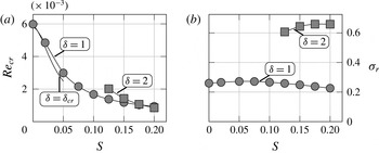
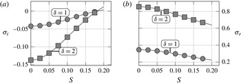
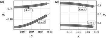
Variations of the critical Reynolds numbers
 $Re_{c}$
of the two most unstable, two-dimensional travelling waves (a) and the corresponding critical frequencies
 $\unicode[STIX]{x1D70E}_{r,c}$
(b) as functions of the groove amplitude
 $S$
for
 $\unicode[STIX]{x1D6FC}=1$
. Computational boxes containing one corrugation wavelength have been used to produce these results.
 $\unicode[STIX]{x1D6FF}=\unicode[STIX]{x1D6FF}_{cr}$
indicates the critical Reynolds number calculated using the immersed boundary conditions (IBC) method (Floryan & Floryan Reference Floryan and Floryan2010) which permits a nearly continuous variations of
 $\unicode[STIX]{x1D6FF}$
.

Assuming that the length of the computational box is
 $L=n\ast \unicode[STIX]{x1D706}$
, where
 $n$
is the number of corrugations contained in the box, the discretized operator can only capture waves with wavelengths
 $L/m$
where
 $m$
is an integer. This limits the disturbance wavelengths which can be captured using this particular box to
 $\unicode[STIX]{x1D6FF}=\unicode[STIX]{x1D6FC}m/n$
, i.e. it is not possible to vary
 $\unicode[STIX]{x1D6FF}$
values in a continuous manner. Nevertheless, useful conclusions regarding characteristics of various waves can be extracted by properly adjusting the length of the computational box. In the analysis, boxes with length
 $L=2\unicode[STIX]{x03C0}$
were used to study waves with
 $\unicode[STIX]{x1D6FF}=1,2,\ldots ,m$
. In the case of
 $\unicode[STIX]{x1D6FC}=3$
, boxes containing
 $n=2$
and
 $5$
corrugations were used to study waves with non-integer
 $\unicode[STIX]{x1D6FF}$
values. Verification of the accuracy of this method is discussed in appendix B. It is known that flow in a smooth channel becomes unstable at
 $Re_{cr}=5772$
and the two-dimensional (TS) wave with the wavenumber
 $\unicode[STIX]{x1D6FF}_{c}=1.02$
travelling downstream plays the critical role. Floryan & Floryan (Reference Floryan and Floryan2010) reports that in the case of small groove amplitudes the critical wavenumber changes marginally. Figure 11(a) illustrates the dependence of the critical Reynolds number on the amplitude
 $S$
determined for
 $\unicode[STIX]{x1D6FC}=1$
using a computational box with length equal to one groove wavelength. Variations of frequencies
 $\unicode[STIX]{x1D70E}_{r}$
of the two dominant instability modes are displayed in figure 11(b). It can be seen that the wave with frequency
 $\unicode[STIX]{x1D70E}_{r}\approx 0.2$
plays the critical role until
 $S$
reaches a certain critical magnitude and then the wave with frequency
 $\unicode[STIX]{x1D70E}_{r}\approx 0.6$
begins to play the critical role. Tracking of frequencies of these two waves in the limit
 $S\rightarrow 0$
demonstrates that they connect to TS waves with the wavenumbers
 $\unicode[STIX]{x1D6FF}=1$
and
 $\unicode[STIX]{x1D6FF}=2$
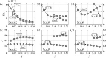
(figure 12). These results suggest that growth of the groove amplitude results in the reduction of the effective channel opening giving preference to waves with shorter wavelengths. Figure 13 illustrates the behaviour of these waves in channels with different corrugation wavenumbers. The critical Reynolds numbers for both waves in channels with long wavelength grooves (
 $\unicode[STIX]{x1D6FC}=0.5$
; see figure 13
a) decrease monotonically as
 $S$
increases. The wave with
 $\unicode[STIX]{x1D6FF}=2$
becomes the dominant one at
 $S\succsim 0.07$
. When the groove wavelength is reduced to
 $\unicode[STIX]{x1D6FC}=5$
(see figure 13
b),
 $Re_{cr}$
for wave with
 $\unicode[STIX]{x1D6FF}=1$
reaches a minimum for
 $S\approx 0.1$
and increases for larger
 $S$
. The wave with
 $\unicode[STIX]{x1D6FF}=2$
begins to dominate for
 $S\succsim 0.12$
. When the groove wavelength is further reduced (see figure 13 for
 $\unicode[STIX]{x1D6FC}=8$
), the non-monotonic variations for
 $Re_{cr}$
for the wave with
 $\unicode[STIX]{x1D6FF}=1$
are more pronounced and amplitude
 $S$
has to reach a higher value before the wave with
 $\unicode[STIX]{x1D6FF}=2$
becomes critical. In this particular case, i.e.
 $\unicode[STIX]{x1D6FC}=8$
, the wave with
 $\unicode[STIX]{x1D6FF}=2$
dominates for
 $S\succsim 0.17$
.
Variations of the amplification rate
 $\unicode[STIX]{x1D70E}_{i}$
(a), and the frequency
 $\unicode[STIX]{x1D70E}_{r}$
(b) of the travelling wave instability for
 $\unicode[STIX]{x1D6FC}=1$
for the two most unstable two-dimensional waves as functions of the groove amplitude
 $S$
for
 $Re=1000$
. Computational boxes containing one corrugation wavelength have been used to produce these results.

Variations of the critical conditions for the two most unstable, two-dimensional waves as functions of the groove amplitude
 $S$
: (a–c) display the critical Reynolds numbers
 $Re_{c}$
for the groove wavenumbers
 $\unicode[STIX]{x1D6FC}=0.5,5,8$
, respectively, and (d–f) display the corresponding critical frequencies
 $\unicode[STIX]{x1D70E}_{r,c}$
. Computational boxes of length
 $2\unicode[STIX]{x03C0}$
have been used to produce these results.

The above results were produced using computational boxes with lengths selected to contain integer numbers of corrugation and waves‘ wavelengths. One should expect continuous variations of the critical
 $\unicode[STIX]{x1D6FF}$
as a function of
 $S$
but this process cannot be followed using the present numerical method. The continuous variations of
 $\unicode[STIX]{x1D6FF}$
are illustrated in qualitative sense in figure 14 for the groove wavenumber
 $\unicode[STIX]{x1D6FC}=3$
. The lengths of the computational boxes have been adjusted to allow for capturing waves with different
 $\unicode[STIX]{x1D6FF}$
values. It can be seen that an increase of
 $S$
gives preference to waves with shorter wavelengths.
Variations of the critical Reynolds number
 $Re_{c}$
(a) and the critical frequency
 $\unicode[STIX]{x1D70E}_{r,c}$
(b) for the least stable two-dimensional travelling waves for the corrugation wavenumber
 $\unicode[STIX]{x1D6FC}=3$
as functions of the corrugation amplitude
 $S$
. Computational boxes with the properly selected lengths have been used to study waves with fractional
 $\unicode[STIX]{x1D6FF}$
values.

3 Three-dimensional flow dynamics
Flow three-dimensionalization in a converging–diverging channel can be caused either by the appearance of the three-dimensional travelling waves or by the formation of streamwise vortices. We shall begin the discussion with the former one.
3.1 Three-dimensional travelling wave
It is known that the two-dimensional waves are less attenuated than the three-dimensional waves in channels with small amplitude of convergence–divergence
 $S$
(Cho et al.
Reference Cho, Kim and Shin1998; Floryan & Floryan Reference Floryan and Floryan2010). It remains to be shown that this relation holds when the amplitude
 $S$
is increased. The solution procedure is identical to that described in § 2.3 with small changes explained below. The disturbances are assumed to be in the form:
 $$\begin{eqnarray}\displaystyle q_{p}(x,y,z,t)=\tilde{\dot{Q}}_{p}(x,y)\text{e}^{\text{i}(\unicode[STIX]{x1D6FF}x+\unicode[STIX]{x1D707}z-\unicode[STIX]{x1D70E}t)}+\text{c.c.} & & \displaystyle\end{eqnarray}$$
resulting in an eigenvalue problem for the partial differential equations describing
 $\tilde{\dot{Q}}_{p}(x,y)$
. One only needs to discretize
 $Q_{p}$
in the
 $(x,y)$
-plane. The discretization process is the same as described in § 2.1 resulting in an algebraic eigenvalue problem where
 $\unicode[STIX]{x1D707}$
and
 $\unicode[STIX]{x1D6FF}$
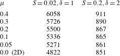
play the role of parameters. Results presented in table 1 demonstrate an increase of the critical Reynolds number as the wave inclination angle increases for small and large amplitudes of corrugation
 $S$
. It can be concluded that it is unlikely that the flow three-dimensionalization can be caused by the three-dimensional travelling waves.
Variations of the critical Reynolds number
 $Re_{cr}$
for oblique travelling waves with the wave vector (
 $\unicode[STIX]{x1D6FF}=1,2$
,
 $\unicode[STIX]{x1D707}$
) as a function of the wave inclination angle expressed in terms of the spanwise wavenumber
 $\unicode[STIX]{x1D707}$
for grooves with
 $\unicode[STIX]{x1D6FC}=1$
.

3.2 Streamwise vortices
We shall now focus our attention on the streamwise vortices. Channel modulations force a change of direction of the flow creating a centrifugal-force field which, under certain conditions, may lead to the formation of a secondary flow in the form of streamwise vortices. As the centrifugal force drives the instability and viscous effects oppose it, the vortices may appear only when the former one dominates, i.e. when the streamline curvature is large enough to generate centrifugal forces strong enough to overcome friction. It is rather obvious that an increase of
 $Re$
will lead to the flow destabilization as larger
 $Re$
signals the reduction of viscous forces. The effects of geometry changes are more difficult to predict without detailed analysis. An initial increase of the groove amplitude increases streamline curvature but an excessive increase leads to flow separation which decreases the curvature. It goes without saying that streamlines of the main stream, and not streamlines inside the separation bubbles, are of consequence.
The conditions leading to the onset of streamwise vortices can be predicted using stability theory. Disturbance quantities are represented using equation (2.23) with
 $\unicode[STIX]{x1D70E}_{r}=0$
since vortices do not propagate, as opposed to the waves. Rather than solving an eigenvalue problem for the disturbance equations, we solve the complete time-dependent problem described by (2.2), where the flow quantities are represented by a Fourier expansion truncated to
 $N$
leading modes, i.e.
 $$\begin{eqnarray}\displaystyle \boldsymbol{u}(x,y,z,t)=\mathop{\sum }_{k=-N}^{k=N}\hat{\boldsymbol{u}}_{k}(x,y,t)\text{e}^{\text{i}k\unicode[STIX]{x1D707}z}, & & \displaystyle\end{eqnarray}$$
where
 $\hat{\boldsymbol{u}}_{k}=\hat{\boldsymbol{u}}_{-k}^{\ast }$
are the reality conditions and stars identify the complex conjugate. The initial conditions consist of a superposition of the two-dimensional solution, determined in § 2.2.2, and a suitable three-dimensional perturbation. The evolution of the perturbations is followed in time by computing the kinetic energy of the Fourier mode of interest defined as
 $$\begin{eqnarray}\displaystyle E_{k}(t)=\frac{1}{2}\int _{\unicode[STIX]{x1D6FA}}\Vert \hat{\boldsymbol{u}}_{k}(t)\Vert ^{2}\,\text{d}\unicode[STIX]{x1D6FA}, & & \displaystyle\end{eqnarray}$$
where
 $k$
denots the mode number. According to (2.23), the energy is expected to vary exponentially, i.e.
 $$\begin{eqnarray}\displaystyle E_{k}(t)=A_{k}\cdot \text{e}^{B_{k}\cdot t}, & & \displaystyle\end{eqnarray}$$
where
 $A_{k}$
and
 $B_{k}$
are constants to be determined. The reader may note that the growth rate for mode
 $k$
can be expressed as
 $\unicode[STIX]{x1D70E}_{i,k}=B_{k}/2$
. The modal functions are discretized on a box of length
 $\unicode[STIX]{x1D706}=2\unicode[STIX]{x03C0}/\unicode[STIX]{x1D6FC}$
using the same spectral finite-element discretization method as used in § 2.2.2. The same temporal discretization as in § 2.2.2 is used to determine the time evolution.
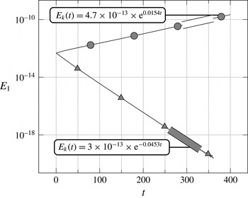
All modes can be traced during time simulation. For each mode a nonlinear least-square fitting of (3.4) to a sample of data is used to determine constants
 $A_{k}$
and
 $B_{k}$
as illustrated in figure 15. Since the first mode is the most unstable (Floryan Reference Floryan2003), and to limit the computational cost, only the zeroth mode (mean flow representation) and the first mode (the dominant disturbance mode) have been traced during the majority of simulations. This limits the results to the linear stability theory. We shall discuss higher modes when discussing saturation states.
Evolution of the kinetic energy of the first Fourier mode (see (3.3)) for flows with
 $Re=500$
and
 $Re=2500$
in a channel with
 $\unicode[STIX]{x1D6FC}=3$
,
 $S=0.05$
,
 $\unicode[STIX]{x1D707}=3.5$
. Solid lines illustrate the complete time history while the thick lines identify the data segments used for determination of
 $A_{k}$
and
 $B_{k}$
(see (3.4)). Computational box containing one corrugation wavelength has been used to produce these results.

Figure 15 illustrates the data fitting process used to determine
 $A_{k}$
and
 $B_{k}$
. Variations of the kinetic energy are plotted as a function of time and the curve fitting produces approximations for the growth rate. Accuracy verification of this procedure is discussed in appendix C.
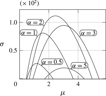
Figure 16 illustrates variations of the amplification rate as a function of the vortex wavenumber
 $\unicode[STIX]{x1D707}$
for corrugations with the amplitude
 $S=0.1$
and with different wavelengths for
 $Re=1300$
. It can be seen that vortices which are either too large or too small are being attenuated. The range of unstable
 $\unicode[STIX]{x1D707}$
is a strong function of
 $\unicode[STIX]{x1D6FC}$
with grooves which are either too long or too short unable to cause the instability. In the former case, the streamline curvature is dictated by the slope of the bounding walls (see figure 2
a). Since this slope is very small, the centrifugal force is too weak to cause the instability. In the latter case, the stream lifts above the grooves (see figure 3) resulting in nearly rectilinear streamlines and a centrifugal force which is also too weak to create the secondary flow.
Variations of the vortex amplification rate as a function of the vortex wavenumber
 $\unicode[STIX]{x1D707}$
for different corrugation wavelengths for
 $Re=1300$
and
 $S=0.1$
. Computational boxes containing one corrugation wavelength have been used to produce these results.

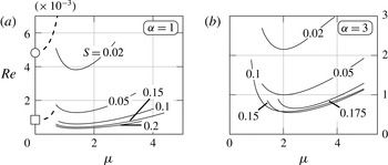
Figure 17 illustrates the neutral curves in the
 $(Re,\unicode[STIX]{x1D707})$
-plane for corrugations with the fixed wavelength
 $\unicode[STIX]{x1D706}=2\unicode[STIX]{x03C0}/\unicode[STIX]{x1D6FC}$
but with the variable amplitude
 $S$
. The minima of these curves determine the critical conditions, i.e. the critical Reynolds numbers
 $Re_{cr}$
and the critical vortex wavenumbers
 $\unicode[STIX]{x1D707}_{cr}$
. It can be seen that an increase of
 $S$
results in negligible variations of
 $\unicode[STIX]{x1D707}_{cr}$
but changes of
 $Re_{cr}$
are more complex and depend on
 $\unicode[STIX]{x1D6FC}$
. In the case of long-wavelength grooves (
 $\unicode[STIX]{x1D6FC}=1$
, figure 17
a), the initial increase of
 $S$
results in a rapid decrease of
 $Re_{cr}$
which eventually saturates with the neutral curves for
 $S=0.15$
and
 $S=0.20$
nearly overlapping. In the case of the grooves with shorter wavelength (
 $\unicode[STIX]{x1D6FC}=3$
, figure 17
b), the initial rapid decrease of
 $Re_{cr}$
is followed by an increase once
 $S$
becomes large enough. In this case, most of the neutral curve for
 $S=0.175$
is above the neutral curve for
 $S=0.15$
. Figure 17(a) also displays the neutral curves for the travelling wave instability. It can be seen that the two-dimensional waves dictate the critical conditions with
 $Re_{cr}$
for the waves being larger than
 $Re_{cr}$
for the vortices.
The neutral stability curves in the
 $(Re,\unicode[STIX]{x1D707})$
-plane for different groove amplitudes
 $S$
. Solid lines correspond to the critical Reynolds numbers for the vortex instability. Dashed lines correspond to the critical Reynolds numbers for the travelling wave instability. ○ Identifies the two-dimensional wave for
 $S=0.02$
and ▫ identifies such wave for
 $S=0.2$
. Computational boxes containing one corrugation wavelength have been used to produce these results.

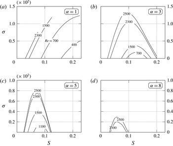
Effects of the groove amplitude are explicitly illustrated in figure 18, which displays variations of the amplification rate for vortices with
 $\unicode[STIX]{x1D707}_{cr}$
as a function of
 $S$
for a fixed
 $Re$
. In all cases the groove amplitude needs to reach a certain minimum before a vortex instability may be initiated. If the groove amplitude is too small, the system response is dominated by the travelling wave instability (Floryan & Floryan Reference Floryan and Floryan2010). In the case of the long-wavelength grooves (
 $\unicode[STIX]{x1D6FC}=1$
, figure 18
a) the vortex amplification rate monotonically increases with
 $S$
up to the maximum
 $S$
considered in this analysis. The vortices can be amplified for
 $Re$
as low as
 $Re\approx 400$
. Reduction of the groove wavelength (
 $\unicode[STIX]{x1D6FC}=3$
, figure 18
b) changes the system response qualitatively as an increase of
 $S$
initially leads to an increase of the amplification followed by its decrease and the eventual vortex stabilization even for the highest
 $Re$
considered. In this case one needs to use at least
 $Re\approx 700$
in order to create this instability. Further reduction of the groove wavelength (
 $\unicode[STIX]{x1D6FC}=5$
, figure 18
c) follows the same trend. One needs to increase the Reynolds number up to
 $Re\approx 1000$
in order to create a secondary flow and the vortex stabilization takes place when
 $S$
increases beyond
 $S\approx 0.12$
. In the case of the short-wavelength grooves (
 $\unicode[STIX]{x1D6FC}=8$
, figure 18
d), one needs to use
 $Re>2000$
to cause the instability, the range of
 $S$
that can lead to instability is very narrow and the amplification rates are very small. Further increase of
 $\unicode[STIX]{x1D6FC}$
eliminates the vortex instability altogether in the range of
 $S$
and
 $Re$
considered.
Variations of the vortex amplification rate at
 $\unicode[STIX]{x1D707}_{cr}$
as a function of the groove amplitude and the flow Reynolds number. Computational boxes containing one corrugation wavelength have been used to produce these results.

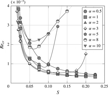
Figure 19 displays variations of the critical Reynolds numbers as a function of the corrugation amplitude. A monotonic decrease of
 $Re_{cr}$
is observed for the longest groove wavelengths tested (
 $\unicode[STIX]{x1D6FC}=0.5,1.0$
). Starting with
 $\unicode[STIX]{x1D6FC}=2$
, one can identify an amplitude
 $S$
which corresponds to the minimum critical Reynolds number. We shall refer to this amplitude as the critical amplitude
 $S_{cr}$
. As the corrugation wavelength further decreases (see curves for
 $\unicode[STIX]{x1D6FC}=3,5,8$
in figure 19), the critical amplitude decreases to about
 $S_{cr}\approx 0.06$
and the minimum
 $Re_{cr}$
increases to approximately
 $Re_{cr}\approx 1800$
. It is worth noticing that further decreases of groove wavelength to
 $\unicode[STIX]{x1D6FC}=10$
do not affect
 $S_{cr}$
but increases the minimum
 $Re_{cr}$
.
Variations of the critical Reynolds number
 $Re_{cr}$
as a function of the groove amplitude
 $S$
. Symbols identify the computed data points. Dotted lines result from the data extrapolation. Computational boxes containing one corrugation wavelength have been used to produce these results.

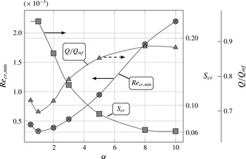
Variations of the minimum critical Reynolds number
 $Re_{cr,min}$
, the corresponding critical corrugation amplitude
 $S_{cr}$
and the corresponding reduction of the flow rate as function of the corrugation wavenumber
 $\unicode[STIX]{x1D6FC}$
. Computational boxes containing one corrugation wavelength have been used to produce these results.

The above results provide a basis for the identification of the most effective geometric configuration for the generation of the vortices. Here we view the configuration which can amplify vortices at the smallest
 $Re$
as being the most effective. Figure 20 displays variations of the minimum critical Reynolds number and the corresponding critical corrugation amplitude
 $S_{cr}$
, as functions of the corrugation wavenumber. Depending on
 $\unicode[STIX]{x1D6FC}$
, the minimum
 $Re_{cr}$
changes from
 $300$
to
 $2200$
and
 $S_{cr}$
changes from
 $0.22$
to
 $0.06$
. The cost of creating vortices can be expressed in terms of the flow rate reduction caused by the grooves. The flow rate reduction corresponding to the use of the optimal configuration varies as a function of
 $\unicode[STIX]{x1D6FC}$
from
 $30\,\%$
to
 $11\,\%$
(see figure 20).
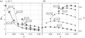
Variations of the critical Reynolds number
 $Re_{cr}$
for the onset of the vortex instability (marked with


 $\unicode[STIX]{x1D6FF}$
as a function of the groove amplitude
 $S$
. Thick solid line without any markers in the insert in (b) has been obtained using IBC method. Data for the vortex instability have been determined using computational boxes containing a single corrugation wavelength. Data for the travelling wave instability have been determined using computational boxes containing different number of corrugation wavelengths; boxes with one corrugation have been used for
 $\unicode[STIX]{x1D6FC}=0.5$
and
 $1$
, boxes with five corrugation wavelengths have been used for
 $\unicode[STIX]{x1D6FC}=5$
, and boxes with two, three and five wavelengths have been used for
 $\unicode[STIX]{x1D6FC}=3$
.

3.3 Competition between the vortices and the travelling waves
The formation of the streamwise vortices is of the main interest in many applications as it results in better flow mixing through creation of transverse fluid motion. The process of vortex creation can be interfered with by the travelling waves. It is thus important to establish conditions where such vortices are likely to dominate the system dynamics. Figure 21 displays variations of
 $Re_{cr}$
as a function of the groove amplitude required for the onset of the travelling waves and for the onset of the vortices. In the case of the long-wavelength grooves (
 $\unicode[STIX]{x1D6FC}=0.5$
, figure 21
a) the vortices dominate in the whole range of corrugation amplitudes being considered in this study with
 $Re_{cr}$
for both instabilities monotonically decreasing as
 $S$
increases, and with
 $Re_{cr}$
for the vortices being always smaller than
 $Re_{cr}$
for the waves. The reader may recall from the discussion in § 2.3 that our method of analysis does not allow for continuous variations of the wavenumber for the travelling wave instability and, thus, the results presented in figure 21 for such waves should be viewed as representing spot checks. The differences between the corresponding
 $Re_{cr}$
and
 $Re_{cr}$
for the vortices are large enough that one can nevertheless conclude that the waves are irrelevant in channels with such corrugations. Reduction of the groove wavelength to
 $\unicode[STIX]{x1D6FC}=1$
(see figure 21
b) leads to a wider separation of
 $Re_{cr}$
with the vortices being more dominant. Further decrease of the groove wavelength to
 $\unicode[STIX]{x1D6FC}=3$
(see figure 21
c) affects very little variations of
 $Re_{cr}$
for the waves but changes the character of variations of
 $Re_{cr}$
for the vortices.
 $Re_{cr}$
in the latter cases initially decreases and then it starts to increase. As a result, the vortices dominate until
 $S\approx 0.17$
and the waves take over for larger
 $S$
. It is unlikely that the vortices can be formed in channels with such large
 $S$
. In the case of the short-wavelength grooves (
 $\unicode[STIX]{x1D6FC}=5$
, figure 21
d) formation of the waves requires the use of
 $Re$
much larger than in the case of
 $\unicode[STIX]{x1D6FC}=3$
while the vortices can be created with
 $Re$
only somewhat larger but only as long as the groove amplitude is not too large. Increase of
 $S$
above 0.12 results in a rapid stabilization of the vortices and the dominance of the waves. The range of
 $S$
which permits the formation of the vortices without interference from the waves is much smaller in such conduits.
4 Saturation states
Growth of an instability activates nonlinear effects which slow down the growth process and lead to the formation of a saturated state. The existing literature identifies oscillatory, aperiodic and chaotic states using a two-dimensional model and corrugation amplitudes much larger than those considered in the present study (Guzmȧn & Amon Reference Guzmȧn and Amon1994; Guzmȧn & Amon Reference Guzmȧn and Amon1996). It is unlikely that saturated states can remain two-dimensional and, as a matter of fact, the existing experimental observations suggest existence of stationary three-dimensional laminar saturated states (Nishimura et al. Reference Nishimura, Yano, Yoshino and Kawamura1990b ; Gschwind et al. Reference Gschwind, Regele and Kottke1995; Mitsudharmadi et al. Reference Mitsudharmadi, Jamaludin, Winoto, Mastny and Perminov2012). The present analysis will address the question of the character of the saturated state. A full three-dimensional analysis is also required in order to determine mixing intensification resulting from the instabilities induced by wall corrugations.
We shall investigate properties of saturated states by following the disturbance growth discussed in § 3 for a much longer time and allowing for nonlinear interactions between different Fourier modes. The flow resolution and time required for the formation of such states are tested by following the evolution of kinetic energies of different Fourier modes, evolution of the flow rate, evolution of different velocity components in selected test points (not shown) as well as evolution of the mixing intensification. The mixing intensity measures the ‘amount’ of flow in the direction perpendicular to the streamwise direction and is defined as
 $$\begin{eqnarray}\displaystyle \left.\begin{array}{@{}c@{}}\displaystyle M_{v}=\frac{1}{\unicode[STIX]{x1D6FA}}\int _{\unicode[STIX]{x1D6FA}}\sqrt{v^{2}}\,\text{d}\unicode[STIX]{x1D6FA},\\ \displaystyle M_{w}=\frac{1}{\unicode[STIX]{x1D6FA}}\int _{\unicode[STIX]{x1D6FA}}\sqrt{w^{2}}\,\text{d}\unicode[STIX]{x1D6FA},\end{array}\right\} & & \displaystyle\end{eqnarray}$$
where the integration is carried out over the whole computational box
 $\unicode[STIX]{x1D6FA}$
. As properties of the saturated states may vary widely depending on the flow conditions, we shall discuss each flow case separately including verification of the accuracy and resolution of the numerical solution.
We begin the discussion with flow at
 $Re=600$
in a channel with corrugation with
 $\unicode[STIX]{x1D6FC}=3$
and
 $S=0.125$
where the two-dimensional state is characterized by a stationary separation. The critical conditions for the onset of vortices are
 $Re_{cr}\approx 540$
,
 $\unicode[STIX]{x1D707}_{cr}\approx 2.26$
and the critical conditions for the travelling waves
 $Re_{cr}\approx 960$
,
 $\unicode[STIX]{x1D6FF}_{cr}\approx 1.5$
(see figure 21
c). Simulations have been performed in a computational box extending over one corrugation wavelength in the streamwise direction and over one vortex wavelength in the spanwise direction with
 $\unicode[STIX]{x1D706}_{\unicode[STIX]{x1D707}}=2\unicode[STIX]{x03C0}/2.25$
(this box size is close to
 $\unicode[STIX]{x1D707}_{cr}$
). The reader should note that our method allows only travelling waves with the wavenumbers equal to multiplicity of
 $3$
resulting in a higher
 $Re_{cr}$
for the travelling wave instability than the actual one. However, since our method precludes the appearance of arbitrary
 $\unicode[STIX]{x1D6FF}$
values, only the vortex instability is active in our computational box. Simulations have been carried out using
 $N=6$
,
 $12$
,
 $18$
,
 $24$
and
 $30$
modes. The character of the saturated state, i.e. determining if this state is stationary or not, is tested using the most accurate solution (
 $N=30$
) by comparing the kinetic energies of different modes at times
 $T_{a}=8000$
and
 $T_{b}=11\,000$
. This difference is defined as
 $$\begin{eqnarray}\displaystyle \unicode[STIX]{x0394}E=\mathop{\sum }_{k=0}^{30}|E_{k}(T_{a})-E_{k}(T_{b})| & & \displaystyle\end{eqnarray}$$
and was found to be less than
 $2\times 10^{-10}$
which demonstrates that the saturated state is stationary. Analysis of variations of the kinetic energies of individual Fourier modes (data not shown) demonstrate that only the first six modes have energies larger than
 $10^{-14}$
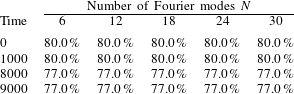
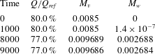
and, thus, use of only the six leading modes provides a sufficient accuracy. Similar conclusions have been reached on the basis of analysis of flow rates (table 2) and mixing intensities (table 3). Most of the computations have been carried out using
 $N=12$
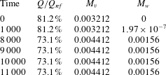
as a precaution. Data presented in table 3 demonstrate that the flow rate decreases marginally compared to the stationary two-dimensional flow while mixing increases in a noticeable manner.
Variations of the flow rate as a function of time counted from the initiation of the instability determined from computations with
 $N$
Fourier modes and expressed as a fraction of the reference flow rate
 $Q_{ref}=4/3$
for channel with
 $\unicode[STIX]{x1D6FC}=3,S=0.125$
for
 $Re=600$
for instability initiated with vortices characterized by
 $\unicode[STIX]{x1D707}=2.25$
.

Variations of the mixing intensities defined by (4.1) and the flow rate
 $Q$
as functions of time counted from the initiation of the instability in a channel with
 $\unicode[STIX]{x1D6FC}=3$
,
 $S=0.125$
for
 $Re=600$
and for the instability initiated with the vortices characterized by
 $\unicode[STIX]{x1D707}=2.25$
determined using
 $N=12$
Fourier modes.

As the second case, we consider flow with
 $Re=1500$
in a channel with a shorter corrugation corresponding to
 $\unicode[STIX]{x1D6FC}=5$
and
 $S=0.1$
. The critical Reynolds number for the vortices is
 $Re_{cr}\approx 998$
and the critical vortex wavenumber is
 $\unicode[STIX]{x1D707}_{cr}\approx 2.7$
. The critical conditions for the travelling wave instability are
 $Re_{cr}\approx 2378$
,
 $\unicode[STIX]{x1D6FF}_{cr}\approx 1$
(see figure 21
d). The saturation analysis is carried out using a computational box of the streamwise length equal to one corrugation wavelength and the spanwise length corresponding to
 $\unicode[STIX]{x1D707}=3.5$
. Only the vortex instability exists for such conditions. Time variations of the kinetic energy of the leading Fourier modes, of the flow rate and of the mixing measures as a function of time (the last two are illustrated in table 4) cannot be detected within numerical accuracy after
 $T=7500$
. The stationary two-dimensional flow has the flow rate
 $Q=1.08$
, i.e.
 $81.2\,\%$
of the flow rate in the smooth channel. The saturated three-dimensional state is reached at
 $T=7500$
and the corresponding flow rate is
 $73.1\,\%$
of the reference flow rate. This state is stationary. The mixing measures show increase in the mixing intensity but smaller than in the flow discussed previously.
The same as table 3, but for
 $\unicode[STIX]{x1D6FC}=5,S=0.1$
,
 $Re=1500$
.

The last case is represented by flow with
 $Re=1000$
in a channel with a longer corrugation corresponding to
 $\unicode[STIX]{x1D6FC}=1$
and
 $S=0.2$
. The critical Reynolds number for the vortices is
 $Re_{cr}\approx 485$
and the critical vortex wavenumber is
 $\unicode[STIX]{x1D707}_{cr}\approx 2.25$
. The critical Reynolds number for the travelling wave instability is
 $Re_{cr}\approx 851$
and the critical wavenumber
 $\unicode[STIX]{x1D6FF}_{cr}\approx 2$
(see figure 21
b). The streamwise length of the computational box corresponds to a single corrugation wavelength and the spanwise length corresponds to
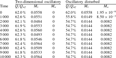
 $\unicode[STIX]{x1D707}=2.25$
. This case is interesting as two two-dimensional states co-exist (see figure 10) i.e. stationary and symmetric flow (§ 2.2.2) with the flow rate approximately 68.67 % of the reference flow rate and the non-symmetric oscillatory flow resulting from the growth of the two-dimensional travelling wave instability (§ 2.3) with the flow rate of approximately 62 % of the reference flow rate. Since the channel’s geometry and the flow conditions promote the growth of the vortex instability, it is possible that the three-dimensional effects could eliminate the flow oscillations.
The first step of the analysis consists of continuing the two-dimensional computations capturing transition to the two-dimensional oscillatory flow (see § 2.3) for a much longer time. Variations of the kinetic energy of the zeroth mode illustrated in figure 22 do not indicate any major changes in the flow as time progresses. The flow rate variations, shown in table 4, oscillate around
 $Q=0.8267$
, i.e.
 $62\,\%$
of the reference flow rate. In the second step, the oscillatory flow was disturbed using a three-dimensional disturbance with the wavenumber
 $\unicode[STIX]{x1D707}=2.25$
. Initial variations of the kinetic energy of the zeroth mode shown in figure 22 demonstrate that the two-dimensional and three-dimensional simulations begin to diverge at
 $T\approx 100$
. In the third step, the initially stationary two-dimensional flow was disturbed using the same three-dimensional disturbance. The evolution of the kinetic energy of the zeroth Fourier mode shown in figure 22 demonstrates that the differences between the initially oscillatory and the initially stationary flows persist for up
 $T\approx 1000$
, as both of them originate from different two-dimensional states, but become negligible for longer times.
Variations of the kinetic energy (3.3) of the zeroth Fourier mode for flows through channel with
 $\unicode[STIX]{x1D6FC}=1,S=0.2$
at
 $Re=1000$
.


 $\unicode[STIX]{x1D707}=2.25$
and the stationary flow modified with the same three-dimensional disturbance.
 $N=12$
Fourier modes have been used. Computational boxes containing one corrugation wavelength have been used in this study.

We shall now discuss the properties of the three-dimensional saturated state reached by disturbing the two-dimensional oscillatory flow. The oscillations have all but disappeared at time
 $T=1000$
and the energies of different Fourier modes increase monotonically at a rather small rate as the flow evolves towards a fully saturated state (details not shown). Data shown in table 5 identify differences between the two-dimensional and three-dimensional saturated states. In the two-dimensional case the flow rate oscillates around
 $62\,\%$
of the reference value, and the
 $y$
-mixing intensity oscillates around
 $M_{v}=0.0558$
. In the three-dimensional case, the flow rate drops to
 $55.8\,\%$
of the reference value at
 $T=1000$
and reaches the saturated value of
 $54.7\,\%$
at
 $T\approx 2000$
.
 $M_{v}$
drops to
 $0.0149$
at
 $T=1000$
and reaches the saturated value of
 $0.0144$
at
 $T\approx 2000$
while
 $M_{w}$
increases to
 $0.0085$
at
 $T=1000$
and reaches the saturated value of
 $0.0082$
at
 $T\approx 2000$
. These results illustrate rapid changes during the initial stage of the flow three-dimensionalization followed by a slow approach to the saturated state. They also demonstrate that the flow three-dimensionalization eliminates oscillations as the final saturated state does not exhibit any time variations.
The same as table 3, but for
 $\unicode[STIX]{x1D6FC}=1,S=0.2$
,
 $Re=1000$
.

Topologies of the saturated states are illustrated in figure 23 displaying isosurfaces of the
 $x$
-component of the vorticity vector. The existence of the streamwise vertical structures is clearly documented. There exist small strong primary vortices located in the converging sections of the channel; these vortices are directly created by the centrifugal instability mechanism and have a limited streamwise extent. Much weaker large vortices in the middle of the channel extend over the whole channel length. These vortices are driven by the primary vortices, i.e. they are driven indirectly by the instability mechanism, but, nevertheless, they are responsible for most of the mixing. Each large vortex appears to have two separate cores, with each core located close to the opposite walls and shifted in the spanwise direction with respect to each other (see figure 23
b). The vortex cores of two adjacent counter-rotating vortices approach each other in the area where the fluid is ejected away from the wall. The fluid expands sideways as it approaches the opposite wall and is drawn by the vortex cores located there. The overall topology can be summarized as formed by vortex pairs, with each vortex of the vortex pair tilted in the spanwise direction but in the opposite sense, with the vortex activity concentrated close to the wall, in the zone where two neighbouring vortex cores approach each other and cooperate to create a strong fluid ejecting motion.
Topology of the saturated flow field at
 $T=10^{4}$
for
 $\unicode[STIX]{x1D6FC}=1$
,
 $S=0.2$
,
 $Re=1000$
. (a) The three-dimensional view of the
 $x$
-component of the vorticity vector and (b) the
 $x$
-direction view. (c) The enlargement of the bottom section of the above plot and (d) the side view of the enlargement;
 $N=12$
Fourier modes have been used in the computations.

The complexity of the flow topology is well illustrated in figure 24 displaying the
 $(y,z)$
cuts through the
 $x$
-component of the vorticity field overlaid with the vector lines of the
 $(y,z)$
component of the velocity vector every
 $1/8$
of the groove wavelength. It is most convenient to begin the discussion with figure 24(f) showing the flow structures at
 $x=5\unicode[STIX]{x1D706}/8$
which is located in the converging section of the channel. The primary vortices located next to the walls are clearly visible as well as one large central secondary vortex. The primary and central vortices rotate in the opposite sense. There are remains of another set of vortices located at approximately
 $y=\pm 0.65$
which we will comment on later. This topology is preserved in the qualitative sense at
 $x=3\unicode[STIX]{x1D706}/4$
(figure 24
g),
 $x=7\unicode[STIX]{x1D706}/8$
(figure 24
h) and
 $x=0,\unicode[STIX]{x1D706}$
(figure 24
a). Downstream from
 $x=0$
the channel begins to expand and the instability mechanism ceases to exist. The distribution of the centrifugal forces is such as it contributes to the attenuation of the vortices in addition to viscous attenuation. The primary vortices created in the converging section remain at approximately the same
 $y$
-elevation but the space between them and the retreating walls is filled in with another layer of vortices rotating in the opposite sense (figure 24
b). One can interpret this process as splitting of the primary vortices into two layers as the space occupied by the central vortex remains nearly the same. The attenuation continues at
 $x=\unicode[STIX]{x1D706}/4$
(figure 24
c) with the thickness and the
 $y$
-locations of the primary vortices remaining the same and with the additional vortices adjacent to the walls expanding in order to fill in the increase of the cross-sectional area created by the channel expansion. The same process leads to breaking up of the remains of the primary vortex into a discontinued set of blobs with the central vortex beginning to merge with the wall-adjacent vortices as illustrated in figure 24(d) for
 $x=3\unicode[STIX]{x1D706}/8$
. As the channel maximum opening is reached, a new generation of primary vortices begins to form in the areas adjacent to the walls (figure 24
e) while the remains of the previous generation continue their decay and the leftover blobs keep shrinking. These blobs still exist at
 $x=5\unicode[STIX]{x1D706}/8$
(figure 24
f) but are completely gone at
 $x=3\unicode[STIX]{x1D706}/4$
(figure 24
g).
Distributions of the
 $x$
-component of the vorticity vector in the (
 $y,z$
) plane overlaid with the vector lines of the (
 $y,z$
) component of the velocity vector at (a)
 $x=0$
, (b)
 $\unicode[STIX]{x1D706}/8$
, (c)
 $\unicode[STIX]{x1D706}/4$
, (d)
 $3\unicode[STIX]{x1D706}/8$
, (e)
 $\unicode[STIX]{x1D706}/2$
, (f)
 $5\unicode[STIX]{x1D706}/8$
, (g)
 $3\unicode[STIX]{x1D706}/4$
and (h)
 $7\unicode[STIX]{x1D706}/8$
. Arrows illustrate the (
 $y,z$
) component of the velocity vector. Dashed lines separate zones with the positive and negative
 $x$
-components of the vorticity vector. Flow and geometry conditions are the same as in figure 23.

Particle trajectories in the saturated flow field for
 $\unicode[STIX]{x1D6FC}=1,S=0.2$
at
 $Re=1000$
. with the instability characterized by
 $\unicode[STIX]{x1D707}=2.25$
. The
 $x$
-direction has been scaled down 10 times. (a) The three-dimensional view, (b) view in the
 $z$
-direction, (c) view in the
 $y$
-direction, (d) view in the negative
 $x$
-direction (only solid black and grey tracers are shown), (e) view in the negative
 $x$
-direction (only dashed black and grey tracers are shown). Traces have been injected into the flow field at the narrowest section of the channel, near the bottom wall (solid black lines), at the mid-plane (solid grey lines) and near the top wall (dashed, black lines).

The character of the mixing processes is illustrated in figure 25 using particle trajectories associated with the velocity field corresponding to
 $T=10\,000$
. The solid black lines, the solid grey lines and the dashed black lines identify trajectories of particles released close to the lower wall, in the middle of the channel and close to the upper wall, respectively. The trajectories of the particles released in the middle of the channel display characteristic convergence corresponding to approximately
 $90$
degrees rotation of the central vortex. This movement is very slow as it takes approximately
 $20$
groove wavelengths to complete this rotation. Particles released close to the walls exhibit rapid convergence as they are placed in the zones where the primary vortices are active. This convergence is completed in just one groove wavelength and is followed by a slow movement away from the walls driven by the central vortices. It takes approximately
 $40$
groove wavelengths for these particles to reach the opposite wall. At this moment a very rapid mixing occurs as the particles re-enter zones affected by the primary vortices. The same sequence of events is repeated when the particles leave these zones and begin to travel back towards the walls where they were released. The reader may note that particles released in the middle of the channel in the spanwise positions away from the edges of the central vortices continue their slow rotation over the whole channel length including the rapid mixing zone described above. This effect is documented by the convergence of the trajectories followed by their divergence, with the maximum divergence occurring in the streamwise location corresponding to the rapid mixing zone, and followed by the next cycle of convergence downstream from this zone. The transverse movement of particles is well documented in figure 25(d,c) displaying views in the negative
 $x$
-direction. The rotational movement of particles released close to each wall is clearly documented as well as the rotational movement of particles released in the middle of the channel. The latter particles released in the zones away from the borders between central vortices remain trapped in the vortex cores. The overall strength of the rotational motion responsible for the transfer of particles between the walls is rather weak as it takes approximately
 $40$
corrugation wavelengths for these particles to traverse the channel height. The flow remains laminar during this mixing process although its form is very complex.
5 Conclusions
The pressure-gradient-driven flow in a converging–diverging channel has been studied. The primary motivation for this analysis is the identification of conduit geometries which can be used for mixing intensification through formation of the streamwise vortices. Such vortices can be induced using the centrifugal instability with a much smaller drag penalty when compared with the vortices created using standard vortex generators.
The model geometry consists of a smooth reference channel modified by transverse sinusoidal grooves with the amplitude
 $S$
and the wavenumber
 $\unicode[STIX]{x1D6FC}$
being the only geometric parameters. The mean openings of the reference smooth channel and of the converging–diverging channel are the same, with the grooves used to produce spatial flow modulations only. The flow is driven by a fixed pressure gradient with the resulting flow rate being a function of the groove geometry. The analysis covers the range of groove wavenumbers being of practical interest, i.e.
 $\unicode[STIX]{x1D6FC}=(0.5,10)$
, and is limited to the groove amplitudes reaching up to 10 % of the channel opening. The analysis is limited to Reynolds numbers resulting in the formation of secondary states and relies on direct numerical simulations combined with linear stability techniques and with the spectral finite element method used for modelling of the channel geometry.
The geometry is two-dimensional but the flow response can be either two-dimensional or three-dimensional depending on the details of the geometry. Accordingly, the analysis consisted of two parts, i.e. the two-dimensional dynamics and the three-dimensional dynamics.
The two-dimensional model demonstrates that an increase of the groove amplitude may result in the formation of separation bubbles whose form is a function of the groove wavenumber. The separation is steady in the case of short groove wavelengths and can be formed using fairly small groove amplitudes. As the groove wavelength increases while the amplitude is kept constant, the separation bubble decreases in size (when measured in terms of a fraction of the groove wavelength), it becomes oscillatory, then it returns to a stationary state and, eventually, the flow separation is completely eliminated. It has been shown analytically that there is no separation for sufficiently long groove wavelengths. The conditions leading to the onset of the oscillatory separation have been determined using linear stability. It has been shown that the onset of the oscillatory separation represents a subcritical Hopf bifurcation associated with the formation of the travelling wave instability. The critical conditions for the onset of this instability have been determined for the complete range of parameters being of interest in this analysis. It has been further demonstrated that multiple flow states may exist under the same geometric and flow conditions.
The three-dimensional model is able to capture the complete flow dynamics. The dynamics is two-dimensional up to the onset of streamwise vortices which lead to the flow three-dimensionalization. Such flow three-dimensionalization is able to eliminate flow oscillations associated with oscillatory separation. The onset conditions have been determined for the geometries of interest in this analysis. It has been shown that the groove wavelength cannot be either too short or too long in order to generate such vortices. In the latter case, the flow modulations are too weak to create a centrifugal-force field strong enough for the flow destabilization. In the former case, the stream lifts up above the grooves and becomes more rectilinear also reducing the strength of the centrifugal-force field. When a groove wavelength from the middle range is used, an increase of the groove amplitude reduces the critical Reynolds number but its excessive increase reverses this trend resulting in the flow stabilization. This effect is related to the flow lift up referred to above. It has been shown that for the groove wavelengths able to produce the vortex instability there exists a most effective groove amplitude which minimizes the critical Reynolds number required for the onset of this instability; either an increase or decrease of the amplitude results in the flow stabilization.
Since the flow in the converging–diverging channel is subject to the competition between the shear-driven and the centrifugal-force-driven instabilities, the geometries giving preference to the vortex instability have been determined. Analysis of saturated states demonstrates that such states are always stationary, even if the primary two-dimensional state is oscillatory. The topologies of the saturated states consist of the primary vortices located next to the walls in the converging channel section and driven directly by the instability mechanism, and secondary vortices filling most of the channel volume. These secondary vortices are responsible for transverse fluid motion which is essential for the increase of the mixing. The transverse fluid movement is fairly slow requiring several groove wavelengths to move fluid elements across the channel.
Acknowledgements
This work has been carried out with support from SHARCNET and the Natural Sciences and Engineering Research Council of Canada (NSERC). SHARCNET of Canada provided the computing resources. We thank Dr H. V. Moradi for providing results of some of the IBC computations.
Appendix A. Analysis of the accuracy of the numerical solution of the two-dimensional stationary problem
The accuracy of the numerical solution is determined through grid convergence studies. Typical results are presented in table 6. The solution error
 $\unicode[STIX]{x1D700}_{i,{\mathcal{X}}}$
is defined as:
 $$\begin{eqnarray}\displaystyle \unicode[STIX]{x1D700}_{i,{\mathcal{X}}}=\frac{1}{N}\mathop{\sum }_{n=1}^{N}\int _{y_{l}(x_{n})}^{y_{u}(x_{n})}(|{\mathcal{X}}_{r}-{\mathcal{X}}_{i}|)\,\text{d}y, & & \displaystyle\end{eqnarray}$$
where
 ${\mathcal{X}}$
stand for any flow quantity, i.e.
 $u$
,
 $v$
,
 $p$
,
 ${\mathcal{X}}_{r}$
stands for the actual value and
 ${\mathcal{X}}_{i}$
stands for the value determined using the grid being tested. The solution obtained using the most refined grid (480 quadrilaterals, seventh-order polynomials) is used as the actual solution. The integration is carried out on
 $N=100$
equally spaced slices from
 $x=0.01\unicode[STIX]{x1D706}$
to
 $x=0.99\unicode[STIX]{x1D706}$
with step size of
 $0.01\unicode[STIX]{x1D706}$
. The integral in (A 1) is evaluated by at first interpolating the discrete data with a cubic spline and then applying the Gauss–Legendre quadrature. Analysis of the results presented in table 6 shows that an acceptable accuracy is obtained using a grid consisting of 120 quadrilaterals combined with the fifth-order polynomials. This grid has been used in most of the computations.
Results of the grid convergence studies for the stationary two-dimensional flow with
 $Re=1500$
in a channel with
 $\unicode[STIX]{x1D6FC}=3$
,
 $S=0.04$
.

Appendix B. Verification of the accuracy of the numerical method used for analysis of the travelling wave instability
To validate the accuracy of the method used to determine the complex amplification rate
 $\unicode[STIX]{x1D70E}$
we start with the smooth channel reference flow. Schmid & Henningson (Reference Schmid and Henningson2012) report that the growth rate for a two-dimensional wave (
 $\unicode[STIX]{x1D707}=0$
) with
 $\unicode[STIX]{x1D6FF}=1$
and
 $Re=2000$
is
 $\unicode[STIX]{x1D70E}=(0.3121003,-0.01979866)$
. The present method implemented with the grid selected in appendix A gives
 $\unicode[STIX]{x1D70E}=(0.312084,-0.0198679)$
. Accuracy for the corrugated channel is verified by comparing
 $\unicode[STIX]{x1D70E}$
values computed using the present method with those computed using the IBC method (Floryan & Floryan Reference Floryan and Floryan2010) and the results are illustrated in figure 26.
Variations of the complex amplification rate
 $\unicode[STIX]{x1D70E}$
as a function of the corrugation amplitude
 $S$
computed using the present method (thin solid line) and the IBC method (Floryan & Floryan Reference Floryan and Floryan2010, thick grey lines) for
 $\unicode[STIX]{x1D6FC}=1$
and
 $Re=1000$
.

Appendix C. Verification of the accuracy of the numerical method used for analysis of the vortex instability
To validate the accuracy of the determination of the amplification rates, we compare the amplification rates determined using time simulations with different time steps with the amplification rates computed by solving an eigenvalue problem using the IBC method (Floryan Reference Floryan2003). The tests use the grid selected in appendix A and the results are presented for the vortex wavenumber
 $\unicode[STIX]{x1D707}=2.25$
.
The amplification rate
 $\unicode[STIX]{x1D70E}_{i}$
for the vortex instability determined using different time steps during the simulation process. The comparison value has been determined by solving the relevant eigenvalue problem using the IBC method (Floryan Reference Floryan2003).

Table 7 illustrates amplification rates determined using different time steps as well as the relative error with respect to the values determined using the IBC method. Application of an excessively large time step results in an attenuation of perturbations and an inability to reproduce the flow physics. Use of the proper time step provides an ability to determine the amplification rate with a sufficient accuracy. Use of an excessively small time step does not necessarily improve the accuracy as the error accumulates over excessively many time steps. Results reported in this paper have been determined using time step
 $10^{-3}$
.
The additional validation step involves comparison of the critical conditions required for the onset of the vortex instability determined using the present method and compared against results obtained using the IBC method (Floryan Reference Floryan2003). Figure 27 displays variations of the critical Reynolds number
 $Re_{cr}$
and the corresponding critical vortex wavenumber
 $\unicode[STIX]{x1D707}_{cr}$
for the corrugation wavenumber
 $\unicode[STIX]{x1D6FC}=3$
as functions of the corrugation amplitude
 $S$
. The IBC method provides an ability to determine the near continuous variations of the critical conditions but is limited by the amplitude of the corrugation that it can handle. The present method can be applied only at discrete points but is not limited by the corrugation amplitude. The discrete data points are marked with symbols in figure 27. The effective resolution is not greater than
 $0.5$
in the
 $\unicode[STIX]{x1D707}$
direction and not greater than
 $100$
in the
 $Re$
direction. The enlargement of the region where both methods are applicable demonstrates that both methods yield nearly the same critical condition. The deviations resulting from the interpolation between the data points determined using the present method are judged to be acceptable.
Variations of the critical conditions
 $(Re_{cr},\unicode[STIX]{x1D707}_{cr})$
for the vortex instability in a channel with the corrugation wavenumber
 $\unicode[STIX]{x1D6FC}=3$
as a function of the corrugation amplitude
 $S$
obtained using the present method as well as the IBC method. The IBC method provides continuous variations of the critical condition for
 $S\in (0,0.05)$
(dashed lines). The present method can be applied for any
 $S$
but provides results only at discrete values of
 $S$
; the computed points are identified using symbols while the solid lines result from interpolation. Dotted lines identify extrapolated values. The box displays enlargement of the region where both methods are equally applicable.