









1. Introduction
Given an extension of fields  $K\subseteq F$ and an element
 $\alpha\in F$, a first interesting question to ask is to determine whether the element α is algebraic over K, i.e. whether it satisfies some non-trivial equation with coefficients in K. In other words, we want to determine whether there exists a non-trivial polynomial
 $p(x)\in K[x]$ such that
 $p(\alpha)=0$. If the answer is affirmative, one tries to study the ideal
 $I_\alpha\subseteq K[x]$ of equations for α over K: this turns out to be a principal ideal, and thus its structure is very simple. Completely analogous questions can be asked in the context of group theory, but the answers turn out to be much more complicated.
Let Fn be a free group generated by n elements  $a_1,...,a_n$. Let
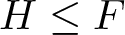
 $H\le F_n$ be a finitely generated subgroup and consider an infinite cyclic group
 $\langle x\rangle\cong\mathbb Z$. An equation in x with coefficients in H is an equality of the form
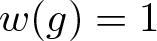
 $w(x)=1$ with
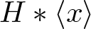
 $w(x)\in H*\langle x\rangle$ in the free product of H and
 $\langle x\rangle$. With an abuse of notation, we will also call the element w(x) an ‘equation’, instead of the equality
 $w(x)=1$. Every
 $w(x)\in H*\langle x\rangle$ has a unique expression as a reduced word in the alphabet
 $\{x,x^{-1}\}\cup H\setminus\{1\}$; we define the degree of w as the number of occurrences of x and x −1 in the cyclic reduction of w. For an element
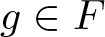
 $g\in F_n$, consider the map
 $\varphi_g:H*\langle x\rangle\rightarrow F_n$ that is the inclusion on H, and that sends x to g; this is the ‘evaluation in g’ map. We say that g is a solution for the equation w if
 $\varphi_g(w)=1$. We define the ideal
 $\mathfrak I_g$ to be the normal subgroup
 $\mathfrak I_g=\ker\varphi_g$ of
 $H*\langle x\rangle$.
First of all, given a finitely generated subgroup  $H\le F_n$, we would like to determine for which elements
 $g\in F_n$ the ideal
 $\mathfrak I_g$ is non-trivial, i.e. which elements satisfy some non-trivial equation over H. This has been answered recently by A. Rosenmann and E. Ventura in [Reference Rosenmann and Ventura14]. Following their terminology, we say that g depends on H if
 $\mathfrak I_g\not=1$ or, equivalently, if
 ${\text{rank}}(\langle H,g\rangle)\le{\text{rank}}(H)$. In [Reference Rosenmann and Ventura14], they provide the following characterization for the elements of Fn that depend on H.
Theorem 1.1 (Rosenmann and Ventura [Reference Rosenmann and Ventura14])
There is an algorithm that, given a finite set of generators for a subgroup  $H\le F_n$, computes a finite set of elements
 $g_1,...,g_k\in F_n$ such that, for every
 $g\in F_n$, the following are equivalent:
(i) The element g depends on H.
(ii) The element g belongs to one of the double cosets
 $Hg_1H,...,Hg_kH$.

Given an arbitrary element  $g\in Hg_iH$ in one of the double cosets as in Theorem 1.1, we have that the ideals
 $\mathfrak I_g$ and
 $\mathfrak I_{g_i}$ are strictly related: if
 $g=hg_ih'$ with
 $h,h'\in H$, then we have that
 $w(x)\in\mathfrak I_g$ if and only if
 $w(hxh')\in\mathfrak I_{g_i}$. This means that, in order to understand the structure of the ideal
 $\mathfrak I_g$ for every element
 $g\in F_n$, it’s enough to focus on the study of the finite family of ideals
 $\mathfrak I_{g_1},...,\mathfrak I_{g_k}$ of the elements
 $g_1,...,g_k$ provided by Theorem 1.1.
In this paper, we fix a finitely generated subgroup  $H\le F_n$ and an element
 $g\in F_n$, and we study the structure of the ideal
 $\mathfrak I_g$. We answer several natural questions about the structure of
 $\mathfrak I_g$, with a particular focus on properties related to the degree of the equations in the ideal. Since the ideal
 $\mathfrak I_g$ can be seen as the kernel of a map between two free groups, it’s possible to algorithmically compute a finite set of generators for
 $\mathfrak I_g$ as normal subgroup of
 $H*\langle x\rangle$ (this is done, for example, in [Reference Kapovich, Myasnikov and Weidmann6]); we describe an algorithm for this purpose, based on Stallings’ folding operations, and we apply it to work out computations in several explicit examples. We show that there is an algorithm that computes a non-trivial equation in
 $\mathfrak I_g$ of minimum possible degree, answering a question asked by A. Rosenmann and E. Ventura; more generally, we show that it’s possible to algorithmically determine whether
 $\mathfrak I_g$ contains equations of a given degree
 $d\in\mathbb N$, and we provide a characterization of all the equations of degree d in
 $\mathfrak I_g$. We also investigate the properties of the set
 $D_g=\{d\in\mathbb N :$ there is a non-trivial equation of degree d in
 $\mathfrak I_g\}$, showing that it coincides, up to a finite set, with either the set of even numbers or with the set of all natural numbers.
In the subsequent paper [Reference Ascari1], we will further investigate the properties of the ideal  $\mathfrak I_g$. In this paper, we make use of techniques based on Stallings’ graphs and folding operations, while in [Reference Ascari1] we deal with the same questions using the theory of context-free languages, a tool which is widely studied in computer science. To the best of our knowledge, some results, such as explicit polynomial bounds on the length of the equations, can only be obtained by means of the folding techniques, while others, such as algorithms running in polynomial time, can only be obtained with context-free languages. We also remark that context-free languages only allow to obtain results for virtually free groups, due to Muller–Shupp theorem, see [Reference Muller and Schupp11]; on the contrary, folding techniques might allow to generalize the results of this paper to wider families of groups.
1.1. Algebraic extensions in free groups
We point out that a notion of algebraic extension in free groups had already been introduced in [Reference Kapovich and Myasnikov5] (see also [Reference Miasnikov, Ventura and Weil10], [Reference Margolis, Sapir and Weil9], [Reference Ventura20]). Given  $H\le J\le F_n$, we say that the extension
 $H\le J$ is algebraic if H isn’t contained in any proper free factor of J. Fixed
 $H\le F_n$ finitely generated, there are only a finite number of subgroups
 $J\le F_n$ such that the extension
 $H\le J$ is algebraic: this follows from the work of Takahasi [Reference Takahasi19]. The notion of algebraic extension is related to the notion of element that depends on a subgroup, as follows. Let
 $H\le F_n$ be a finitely generated subgroup and let
 $g\in F_n$ be an element: then g depends on H if and only if the extension
 $H\le\langle H,g\rangle$ is algebraic. However, we also point out that it’s possible to find an algebraic extension
 $H\le J$ and an element
 $g\in J$ such that g doesn’t depend on H; in this sense, the notion of algebraic extension and the notion of dependence on a subgroup aren’t equivalent. In [Reference Miasnikov, Ventura and Weil10], they also introduce a notion of element algebraic over a subgroup. Given
 $H\le F_n$ and
 $g\in F_n$ we say that g is Fn-algebraic over H if every free factor of Fn containing H also contains g. We point out that, if g depends on H, then g is Fn-algebraic over H, but the converse isn’t true in general.
1.2. Results and structure of the paper
Let Fn be a finitely generated subgroup on n generators  $a_1,...,a_n$; let
 $H\le F_n$ be a finitely generated subgroup and let
 $g\in F_n$ be an element. In this paper, we study the structure of the ideal
 $\mathfrak I_g$ of the equations with coefficients in H with g as a solution. Most of our results can be generalized to equations in more variables, but, for simplicity of notation, for most of the paper we deal only with the one-variable case; the results in the multi-variate setting can be found in
 $\S$ 7 at the end of the paper.
For an arbitrary surjective homomorphism from a finitely generated free group to a finitely presented group, the kernel is always finitely generated as a normal subgroup. If the target is free, then it follows from Grushko’s Theorem that there is an algorithm to find a finite normal generating set; the reader can also refer to [Reference Kapovich, Myasnikov and Weidmann6] for such an algorithm. In  $\S$ 3, we describe an efficient algorithm; the key idea, based on Stallings folding operations, is the following. In a chain of folding operations, the rank-preserving folding operations are homotopy equivalences, and thus isomorphisms at the level of fundamental group, while the non-rank-preserving folding operations give a non-injective map of fundamental groups (that means, in our case, adding generators to the kernel). The novel aspect of our algorithm, which is explained in
 $\S$ 3, is the following: we show that the non-rank-preserving folding operations can be postponed until the end of the chain of folding operations (see Figure 4). This gives a clean and efficient way to produce a set of generators for the kernel as a normal subgroup (which, in the particular case of the map
 $\varphi_g:H*\langle x\rangle\rightarrow F_n$, is exactly the ideal
 $\mathfrak I_g$).
In [Reference Rosenmann and Ventura14], Rosenmann and Ventura ask the following question:
Questions 1.2
Is it possible to (algorithmically) find an equation of minimum degree for an element g that depends on H?
In  $\S$ 4, we give an affirmative answer to this question.
Theorem A (See Corollary 4.13)
There is an algorithm that, given a finite set of generators for a subgroup  $H\le F_n$ and an element
 $g\in F_n$ such that g depends on H, produces a non-trivial equation
 $w\in\mathfrak I_g$ of minimum possible degree.
We give a brief outline of the proof of Theorem A. We take a non-trivial (cyclically reduced) equation  $w\in\mathfrak I_g$ of minimum possible degree; we think of w as a word in the letters
 $a_1,...,a_n,x$ (where
 $a_1,...,a_n$ is a basis for Fn). We then prove that, for words of sufficient length, some parts of the word w can be literally cut away, by means of a move that we call a ‘parallel cancellation move’, introduced in Lemma 4.10; this produces another equation
 $w'\in\mathfrak I_g$, which is strictly shorter than w and which has the same degree. By iterating this process, we prove that there is a (computable) bound
 $B=B(H,g)\ge0$ such that there is an equation in
 $\mathfrak I_g$ of minimum possible degree and with length at most B, see Theorem 4.4 for the precise value of B. With this bound established, the algorithm now just takes all the (finitely many) elements of
 $H*\langle x\rangle$ which are of length at most B, and for each of them it checks whether it belongs to
 $\mathfrak I_g$, recording its degree.
A completely analogous result holds for equations of any fixed degree d: if  $\mathfrak I_g$ contains a non-trivial equation of degree d, then it contains one whose length is bounded (see Theorem 5.12 for the precise bound). In particular, we prove the following theorem:
Theorem B (See Corollary 5.13)
There is an algorithm that, given a finite set of generators for a subgroup  $H\le F_n$, an element
 $g\in F_n$ and an integer
 $d\ge1$, tells us whether
 $\mathfrak I_g$ contains non-trivial equations of degree d, and, if so, produces an equation
 $w\in\mathfrak I_g$ of degree d.
One of the interesting features of the algorithm is that the ‘parallel cancellation moves’ of Lemma 4.10 have inverses, namely the ‘parallel insertion moves’ which we introduce in Lemma 5.4. This means that there is a (computable) bound  $C=C(H,g)\ge0$ such that every (cyclically reduced) equation of degree d can be obtained from an equation of degree d whose length is at most C, by means of a finite number of insertion moves; this gives a characterization of all the equations of degree d in terms of a finite number of short equations (see Theorem 5.14 for the details).
Next, we study the set Dg of degrees of equations with coefficients in H and having g as a solution. We prove that Dg coincides with either  $\mathbb N$ or
 $2\mathbb N$ (the set of non-negative and non-negative even numbers, respectively), up to a finite set. We provide an algorithm that, given H and g, computes the set Dg.
Theorem C (See Theorem 5.17)
Exactly one of the following possibilities takes place:
(i) Dg contains an odd number and
$\mathbb N\setminus D_g$ is finite.(ii) Dg contains only even numbers and
$2\mathbb N\setminus D_g$ is finite.


Theorem D (See Theorem 5.19)
There is an algorithm that, given a finite set of generators for a subgroup  $H\le F_n$ and an element
 $g\in F_n$ that depends on H, produces the following outputs:
(i) Determines whether we fall into case (i) or (ii) of Theorem 5.17.
(ii) Computes the finite set
$\mathbb N\setminus D_g$ or $2\mathbb N\setminus D_g$ respectively.


In  $\S$ 6, we make use of the tools developed in the rest of the paper in order to work out explicit computations in some specific cases; in each case, we compute the minimum degree
 $d_{\min}$ for an equation in
 $\mathfrak I_g$ and the set Dg of possible degrees. In example 6.1, we deal with the case where
 ${\text{rank}}(H)=1$, showing that in this case
 $d_{\min}$ is either 1 or 2. The examples of
 $\S$ 6.2 and 6.3 show that both cases of Theorem C can occur. One may be tempted to conjecture that the equations of
 $\mathfrak I_g$ of minimum possible degree
 $d_{\min}$ are enough to generate the ideal
 $\mathfrak I_g$; we give counterexamples to this (see
 $\S$ 6.3 and 6.4), showing that the ideal
 $\mathfrak I_g$ is not always generated by just the equations of degree
 $d_{\min}$.
In  $\S$ 7, we generalize most of the results of the paper to equations in more variables.
2. Preliminaries and notations
In this section, we introduce the notation about graphs that we are going to use along the paper.
2.1. Graphs and paths
We consider graphs as combinatorial objects, following the notation of [Reference Stallings18] and [Reference Serre15]. A graph Γ is a quadruple  $(V,E,\overline{\cdot},\iota)$ consisting of a set
 $V=V(\Gamma)$ of vertices, a set
 $E=E(\Gamma)$ of edges, a map
 $\overline{\cdot}:E\rightarrow E$ called reverse and a map
 $\iota:E\rightarrow V$ called initial endpoint; we require that, for every edge
 $e\in E$, we have
 $\overline{e}\not=e$ and
 $\overline{\overline{e}}=e$. For an edge
 $e\in E$, we denote with
 $\tau(e)=\iota(\overline{e})$ the terminal endpoint of e.
A map of graphs  $f:\Gamma\rightarrow\Gamma\prime$ is just a couple of maps, vertices to vertices and edges to edges, preserving the reverse and the initial endpoint. A subgraph of a graph Γ is a graph
 $\Gamma\prime\prime$ such that
 $V(\Gamma\prime\prime)\subseteq V(\Gamma)$ and
 $E(\Gamma\prime\prime)\subseteq E(\Gamma)$ and the reverse and endpoint maps on
 $\Gamma\prime\prime$ are the restrictions of the maps on Γ.
A path in a graph Γ, with initial endpoint  $u\in V(\Gamma)$ and terminal endpoint
 $v\in V(\Gamma)$, is a sequence
 $\sigma=(e_1,...,e_\ell)$ of edges
 $e_1,...,e_\ell\in E(\Gamma)$ for some integer
 $\ell\ge0$, with the conditions
 $\iota(e_1)=u$ and
 $\tau(e_\ell)=v$ and
 $\tau(e_i)=\iota(e_{i+1})$ for
 $i=1,...,\ell-1$. The integer
 $\ell$ is called length of the path. For
 $\ell=0$, for every vertex v of Γ there is a unique path of length 0 whose initial and terminal endpoints coincide and are equal to v; we call it the constant path at v. A graph is connected if for every couple of vertices there is a path going from one to the other.
Given two paths  $\sigma=(e_1,...,e_\ell)$ from u to v and
 $\sigma'=(e_1',...,e_{\ell'}')$ from v to w we define their concatenation as the path
 $\sigma\cdot\sigma'=(e_1,...,e_\ell,e_1',...,e_{\ell'}')$ form u to w. Given a path
 $\sigma=(e_1,...,e_\ell)$ from u to v we define its reverse as the path
 $\overline{\sigma}=(\overline{e}_\ell,...,\overline{e}_1)$ from v to u. Given a map of graphs
 $f:\Gamma\rightarrow\Gamma\prime$ and a path
 $\sigma=(e_1,...,e_\ell)$ from u to v in Γ, we define the path
 $f_*(\sigma)$ from f(u) to f(v) in
 $\Gamma\prime$ given by
 $f_*(\sigma)=(f(e_1),...,f(e_\ell))$. The image of a path σ is the smallest subgraph of Γ containing all the edges
 $e_1,...,e_\ell$ (or the single vertex v in case of the constant path at v).
A path  $(e_1,...,e_\ell)$ is reduced if
 $e_i\not=\overline{e}_{i+1}$ for every
 $i\in\{1,...,\ell-1\}$. A path
 $(e_1,...,e_\ell)$ is closed if
 $\tau(e_\ell)=\iota(e_1)$, i.e. if its two endpoints coincide. A closed path
 $(e_1,...,e_\ell)$ is cyclically reduced if it’s reduced and
 $e_\ell\not=\overline{e}_1$. A tree is a connected graph that doesn’t contain any cyclically reduced closed path; we have that, in a tree, every couple of vertices is connected by a unique reduced path.
2.2. Geometric realization and fundamental group
Let  $\Gamma=(V,E,\overline{\cdot},\iota)$ be a graph. The geometric realization
 $|\Gamma|$ is the one-dimensional CW complex that has one 0-cell for every vertex
 $v\in V$ and one 1-cell for every pair of reverse edges
 $\{e,\overline{e}\}\subseteq E$; the 1-cell corresponding to the pair
 $\{e,\overline{e}\}$ has its two endpoints glued onto the vertices
 $\iota(e)$ and
 $\tau(e)$. A map of graphs
 $f:\Gamma\rightarrow\Gamma\prime$ induces a cellular map
 $|f|:|\Gamma|\rightarrow|\Gamma\prime|$ between the geometric realizations. A subgraph
 $\Gamma\prime\prime\subseteq\Gamma$ induces a subcomplex
 $|\Gamma\prime\prime|\subseteq|\Gamma|$.
A path  $\sigma=(e_1,...,e_\ell)$ for
 $\ell\ge1$ induces a continuous map
 $|\sigma|:[0,1]\rightarrow|\Gamma|$: this sends the point
 $\frac{i}{\ell}$ to the vertex
 $\tau(e_{i-1})=\iota(e_i)$ for
 $i=0,...,\ell$, and the interval
 $[\frac{i-1}{\ell},\frac{i}{\ell}]$ to the 1-cell corresponding to the edge ei. We denote with
 $[\sigma]$ the homotopy class (relative to the endpoints) of the geometric realization
 $|\sigma|$. We say that a path σ is homotopically trivial if the homotopy class
 $[\sigma]$ contains a constant path (in particular the two endpoints of σ have to coincide).
Definition 2.1. For a finite graph Γ, define  $\|\Gamma\|:=|E(\Gamma)|/2$ as the number of 1-cells in the geometric realization
 $|\Gamma|$.
Let Γ be a graph. Every covering space of  $|\Gamma|$ can be seen as the geometric realization
 $|q|:|\Gamma\prime|\rightarrow|\Gamma|$ of some map of graphs
 $q:\Gamma\prime\rightarrow\Gamma$; with an abuse of notation, we will call covering map also the map of graphs q (and not only its geometric realization
 $|q|$). In particular, we can consider the universal cover
 $p:\widetilde{\Gamma}\rightarrow\Gamma$; the graph
 $\widetilde{\Gamma}$ is a tree.
Proposition 2.2. Let Γ be a connected graph and let c be a homotopy class of paths in  $|\Gamma|$ relative to the endpoints. Then there is a unique reduced path σ such that
 $[\sigma]=c$.
Sketch of proof
This is a standard application of the theory of covering spaces. Let  $p:\widetilde{\Gamma}\rightarrow\Gamma$ be the universal cover, let
 $\gamma:[0,1]\rightarrow|\Gamma|$ be a path in the homotopy class c and let
 $v_0=\gamma(0)$ and
 $v_1=\gamma(1)$. Choose
 $\widetilde{v}_0\in p^{-1}(v_0)$, let
 $\widetilde{\gamma}:[0,1]\rightarrow|\widetilde{\Gamma}|$ be the unique lifting of γ such that
 $\widetilde{\gamma}(0)=\widetilde{v}_0$ and let
 $\widetilde{v}_1=\gamma(1)$.
The map p induces a bijection between paths  $\widetilde{\sigma}$ in
 $\widetilde{\Gamma}$ from
 $\widetilde{v}_0$ to
 $\widetilde{v}_1$ and paths σ in Γ with
 $[\sigma]=c$; moreover, reduced paths
 $\widetilde{\sigma}$ are in bijection with reduced paths σ. In particular, since
 $\widetilde{\Gamma}$ is a tree, there is a unique reduced path in
 $\widetilde{\Gamma}$ from
 $\widetilde{v}_0$ to
 $\widetilde{v}_1$, and thus a unique reduced path in the homotopy class c.
A pointed graph  $(\Gamma,*)$ is a graph Γ together with a marked vertex
 $*\in V(\Gamma)$. For a pointed graph
 $(\Gamma,*)$ we define its fundamental group
 $\pi_1(\Gamma,*)$ to be the fundamental group
 $\pi_1(|\Gamma|,*)$ of its geometric realization.
We shall need to work explicitly with the following well-known construction. Let  $(\Gamma,*)$ be a finite connected pointed graph and let T be a maximal tree contained in Γ. Let E ʹ be the set of edges which are not contained in T; for each pair of reverse edges
 $\{e,\overline{e}\}\subseteq E'$ choose one of the two elements, let’s say e, and consider the reduced path σe that starts at
 $*$, moves to
 $\iota(e)$ along T, crosses e and goes back from
 $\tau(e)$ to
 $*$ along T.
Proposition 2.3. The fundamental group  $\pi_1(\Gamma,*)$ is a free group with a basis given by the homotopy classes
 $[\sigma_e]$ for each pair of reverse edges
 $\{e,\overline{e}\}\subseteq E'$.
Sketch of proof
We consider the CW complex  $|\Gamma|$ and we collapse the subcomplex
 $|T|$, obtaining a bouquet of circles, one for each pair of reverse edges
 $\{e,\overline{e}\}\subseteq E'$. This induces an isomorphism at the level of the fundamental groups, since the subcomplex
 $|T|$ is contractible. In the bouquet of circles, the image of
 $|\sigma_e|$ crosses the 1-cell corresponding to the pair
 $\{e,\overline{e}\}$ exactly once, and it doesn’t cross any other 1-cell. The result follows by induction on the number of circles, using van Kampen’s theorem.
We will also need the following basic operation between graphs.
Definition 2.4. Let  $(\Gamma,*),(\Delta,*)$ be pointed graphs. Define their join as the pointed graph
 $(\Gamma\vee\Delta,*)$ given by quotient of their disjoint union by the relation that identifies their two basepoints.
We have a natural isomorphism  $\pi_1(\Gamma\vee\Delta,*)=\pi_1(\Gamma,*)*\pi_1(\Delta,*)$.
2.3. Core and pointed core of a graph
Let  $(\Gamma,*)$ be a connected pointed graph: define the pointed core of Γ, denoted by
 ${\text{core}}_*(\Gamma)$, as the subgraph given by the union of the images of all the reduced paths from the basepoint to itself. Notice that
 ${\text{core}}_*(\Gamma)$ is connected, and the inclusion
 ${\text{core}}_*(\Gamma)\rightarrow\Gamma$ induces an isomorphism of fundamental groups
 $\pi_1({\text{core}}_*(\Gamma),*)\rightarrow\pi_1(\Gamma,*)$.
Similarly, let Γ be a connected graph which is not a tree: define the core of Γ, denoted by  ${\text{core}}(\Gamma)$, as the subgraph given by the union of the images of all the closed cyclically reduced non-constant paths. The graph
 ${\text{core}}(\Gamma)$ is connected. If
 $(\Gamma,*)$ is a pointed graph then
 ${\text{core}}(\Gamma)$ is contained in
 ${\text{core}}_*(\Gamma)$ as a subgraph; to be precise, there is a unique shortest path γ (possibly a constant path) connecting the basepoint to
 ${\text{core}}(\Gamma)$; the graph
 ${\text{core}}_*(\Gamma)$ consists exactly of the union of
 ${\text{core}}(\Gamma)$ and of the image of γ.
2.4. Reduction of paths
Let Γ be a graph, let  $\sigma=(e_1,...,e_\ell)$ be a path and suppose σ isn’t reduced. Then we have
 $e_{s+1}=\overline{e}_s$ for some
 $s\in\{1,...,\ell-1\}$, and we can define the path
 $\sigma'=(e_1,...,e_{s-1},e_{s+2},...,e_\ell)$; we say that
 $\sigma'$ is obtained from σ by means of an elementary reduction. Notice that if σ had length
 $\ell$ then
 $\sigma'$ has length
 $\ell-2$; moreover we have
 $[\sigma']=[\sigma]$, i.e. their geometric realizations are homotopic relative to the endpoints. If the path
 $\sigma'$ is not yet reduced, then we can reiterate the same process; this motivates the following definition:
Definition 2.5. Let Γ be a graph and let  $\sigma=(e_1,...,e_\ell)$ be a path. A reduction process for σ is a sequence
 $(s_1,t_1),...,(s_m,t_m)$ for
 $m\in\mathbb N$ with the following properties:
(i)
$s_1,t_1,...,s_m,t_m$ are pairwise distinct integers in $\{1,...,\ell\}$.(ii) For every
$i=1,...,m$ we have $s_i \lt t_i$.(iii) For every
$i=1,...,m$ we have $\{s_i+1,s_i+2,...,t_i-2,t_i-1\}\subseteq\{s_1,t_1,...,s_{i-1},t_{i-1}\}$.(iv) For every
$i=1,...,m$ we have $e_{s_i}=\overline{e}_{t_i}$.


Think of  $e_{s_i},e_{t_i}$ as the ith elementary reduction to be performed on the path σ. Condition (iii) says that the edges
 $e_{s_1},e_{t_1},...,e_{s_{i-1}},e_{t_{i-1}}$ cover interval from
 $e_{s_i}$ to
 $e_{t_i}$, so that, after performing the first i − 1 cancellations, the edges
 $e_{s_i}$ and
 $e_{t_i}$ become adjacent; in particular, s 1 and t 1 have to be consecutive numbers. Condition (iv) ensures that the ith elementary reduction can actually be performed. Condition (ii) is just a useful convention, saying that the edges
 $e_{s_i},e_{t_i}$ appear in this order along the path.
Lemma 2.6. Let Γ be a graph and let  $\sigma=(e_1,...,e_\ell)$ be a path, together with a reduction process
 $(s_1,t_1),...,(s_m,t_m)$. Then for every
 $1\le\alpha \lt \beta\le m$ we have that either
 $s_\alpha \lt t_\alpha \lt s_\beta \lt t_\beta$ or
 $s_\beta \lt t_\beta \lt s_\alpha \lt t_\alpha$ or
 $s_\beta \lt s_\alpha \lt t_\alpha \lt t_\beta$.
Proof. We have  $\{s_\alpha+1,s_\alpha+2,...,t_\alpha-2,t_\alpha-1\}\subseteq\{s_1,t_1,...,s_{\alpha-1},t_{\alpha-1}\}$ and in particular neither sβ nor tβ can occur in the interval
 $\{s_\alpha,s_\alpha+1,...,t_\alpha-1,t_\alpha\}$. The conclusion follows.
Let σ be a path and let  $(s_1,t_1),...,(s_m,t_m)$ be a reduction process for σ. Then we can remove the edges
 $e_{s_1},e_{t_1},...,e_{s_m},e_{t_m}$ from σ in order to obtain a well-defined path
 $\sigma'$. This is the same as performing on σ the sequence of elementary reductions given by the couples
 $(s_i,t_i)$ for
 $i=1,...,m$. We say that
 $\sigma'$ is the residual path of the reduction process. In this case, we have
 $[\sigma']=[\sigma]$, i.e. their geometric realizations are homotopic relative to the endpoints.
Proposition 2.7. Let Γ be a graph and let  $\sigma=(e_1,...,e_\ell)$ be a path, together with a reduction process
 $(s_1,t_1),...,(s_m,t_m)$. Then exactly one of the following holds:
(i) The residual path
$\sigma'$ is reduced.(ii) There is a couple
$(s_{m+1},t_{m+1})$ such that $(s_1,t_1),...,(s_m,t_m),(s_{m+1},t_{m+1})$ is a reduction process for σ.


Proof. Suppose that the residual path  $\sigma'$ isn’t reduced. Then there are integers
 $s',t'\in\{1,...,\ell\}\setminus\{s_1,t_1,...,s_m,t_m\}$ such that
 $s' \lt t'$ and
 $e_{s'}=\overline{e}_{t'}$ and
 $e_{s'}$ and
 $e_{t'}$ are adjacent when seen as edges of the residual path
 $\sigma'$. This means that
 $\{s'+1,s'+2,...,t'-2,t'-1\}\subseteq\{s_1,t_1,...,s_m,t_m\}$, and in particular we can define the couple
 $(s_{m+1},t_{m+1}):=(s',t')$ and this provides a reduction process
 $(s_1,t_1),...,(s_m,t_m),(s_{m+1},t_{m+1})$ for σ, as desired.
The above proposition essentially says that a reduction process can be inductively extended, until we get a residual path which is reduced. A reduction process  $(s_1,t_1),...,(s_m,t_m)$ is called maximal if it can’t be extended by adding a couple of edges
 $(s_{m+1},t_{m+1})$, i.e. if it falls into case (i) of Proposition 2.7. Of course, every path admits at least one maximal reduction process. Despite the maximal reduction process not being unique in general, it turns out that the residual path is unique, as shown in the following proposition:
Proposition 2.8. Let σ be a path in Γ, and let  $\sigma'$ be the unique reduced path such that
 $[\sigma']=[\sigma]$, as in Proposition 2.2. Then every maximal reduction process
 $(s_1,t_1),...,(s_m,t_m)$ for σ has the same residual path, that coincides with
 $\sigma'$.
Proof. The residual path of the process is a reduced path in the homotopy class  $[\sigma]$. But by Proposition 2.2, there is a unique such path. The conclusion follows.
The following graphical representation of a reduction process will be useful. Let  $\sigma=(e_1,...,e_\ell)$ be a path in the graph Γ and let
 $(s_1,t_1),...,(s_m,t_m)$ be a reduction process for σ. Consider the interval
 $[0,1]\times\{0\}\subseteq\mathbb R^2$ and subdivide it at the points
 $(\frac{1}{\ell},0)...,(\frac{\ell-1}{\ell},0)$, and let zj be the midpoint of the segment
 $[\frac{j-1}{\ell},\frac{j}{\ell}]\times\{0\}$ for
 $j=1,...,\ell$. For every couple
 $(s_i,t_i)$, take a smooth curve ri in the upper half-plane connecting
 $z_{s_i}$ to
 $z_{t_i}$. The curves
 $r_1,...,r_m$ can be taken to be pairwise disjoint, as in Figure 1.
An example of a possible diagram for a reduction process. The labels below the interval put in evidence a couple  $(s_i,t_i)$ of the reduction process.

2.5. Labelled graphs
We consider the finitely generated free group Fn of rank n, generated by  $a_1,...,a_n$. For an element
 $h\in F_n$ we denote with
 $\overline{h}=h^{-1}$ the inverse of h. We denote with
 $\Delta_n$ the graph with one vertex
 $V=\{*\}$ and edges
 $E=\{a_1,\overline{a}_1,...,a_n,\overline{a}_n\}$. The fundamental group
 $\pi_1(\Delta_n,*)$ will be identified with Fn: the path
 $\sigma_i=(a_i)$ from
 $*$ to
 $*$ corresponds to the element
 $a_i\in F_n$.
Definition 2.9. A labelled graph is a graph Γ together with a map of graphs  $f:\Gamma\rightarrow \Delta_n$.
This means that every edge of Γ is equipped with a label in  $\{a_1,\overline{a}_1,...,a_n,\overline{a}_n\}$, according to which edge of
 $\Delta_n$ it is mapped to, reverse edges having inverse labels; the map
 $f:\Gamma\rightarrow \Delta_n$ is called labelling map for Γ.
Definition 2.10. Let  $\Gamma_0,\Gamma_1$ be labelled graphs with labelling maps
 $f_0,f_1$ respectively. A map of graphs
 $h:\Gamma_0\rightarrow \Gamma_1$ is called label-preserving if
 $f_1\circ h=f_0$.
2.6. Core graph of a subgroup
From the theory of covering spaces, we know that pointed covering spaces of  $\Delta_n$ are in bijection with subgroups of the fundamental group
 $\pi_1(\Delta_n,*)=F_n$. Given a pointed covering space
 $p:(\Gamma,*)\rightarrow(\Delta_n,*)$, we have that the map
 $p_*:\pi_1(\Gamma,*)\rightarrow F_n$ is injective, and thus
 $\pi_1(\Gamma,*)$ can be identified with its image
 $p_*(\pi_1(\Gamma,*))=H$, determining a subgroup
 $H\le F_n$. Conversely, given a subgroup
 $H\le F_n$, there is a unique pointed covering space
 $p:(\Gamma,*)\rightarrow(\Delta_n,*)$ such that
 $p_*(\pi_1(\Gamma,*))=H$: we define
 $({\text{cov}}(H),*)=(\Gamma,*)$ to be such covering space.
Remark 2.11. A covering space  $p:(\Gamma,*)\rightarrow(\Delta_n,*)$ is in particular a labelled graph.
Definition 2.12. Define the core of H, denoted by  ${\text{core}}(H)$, and the pointed core of H, denoted by
 ${\text{core}}_*(H)$, to be the core and the pointed core of
 $({\text{cov}}(H),*)$, respectively.
Of course  ${\text{cov}}(H),{\text{core}}(H),{\text{core}}_*(H)$ are labelled graphs, with labelling map given by the covering projection p, and by its restriction to the subgraphs
 ${\text{core}}(H)$ and
 ${\text{core}}_*(H)$ respectively. The labelling map
 $f:{\text{core}}_*(H)\rightarrow \Delta_n$ gives a map
 $f_*:\pi_1({\text{core}}_*(H),*)\rightarrow F_n$ which induces an isomorphism
 $f_*:\pi_1({\text{core}}_*(H),*)\rightarrow H$.
We have that H is finitely generated if and only if  ${\text{core}}(H)$ is finite (and if and only if
 ${\text{core}}_*(H)$ is finite). In that case,
 ${\text{core}}(H)$ and
 ${\text{core}}_*(H)$ can be built algorithmically from a finite set of generators for H, see Algorithm 5.4 in [Reference Stallings18].
3. Equations and Stallings folding
It is well-known that, given an homomorphism between finitely generated free groups  $\varphi:F_r\rightarrow F_n$, there is a free factor decomposition
 $F_r=F*F'$ such that φ is injective on F and trivial on F ʹ. We here introduce an efficient way of computing such a decomposition. The technique is based on the classical Stallings folding operations; the novel aspect of what we do is that we focus on the non-rank-preserving folds, which are the ones responsible for the generators of the kernel, and we delay them until the end of the chain of folding operations. In particular, this can be applied to compute, for a given subgroup
 $H\le F_n$ and a given element
 $g\in F_n$, a set of generators of the ideal
 $\mathfrak I_g\trianglelefteq H*\langle x\rangle$ as a normal subgroup.
3.1. Stallings folding operations
We will assume that the reader has some confidence with the classical Stallings folding operation, for which we refer to [Reference Stallings18]. We briefly recall the main properties that we are going to use.
Let Γ be a finite connected labelled graph and suppose there are two distinct edges  $e_1,e_2$ with the same label and with a common endpoint
 $v=\iota(e_1)=\iota(e_2)$. We can identify e 1 with e 2 (and
 $\overline{e}_1$ with
 $\overline{e}_2$, and
 $v_1=\tau(e_1)$ with
 $v_2=\tau(e_2)$): we obtain a label-preserving quotient map of graphs
 $q:\Gamma\rightarrow \Gamma\prime$.
Definition 3.1. The quotient map  $q:\Gamma\rightarrow \Gamma\prime$ is called Stallings folding.
Given a finite connected labelled graph Γ, we can successively apply folding operations to Γ in order to get a sequence  $\Gamma=\Gamma^0\rightarrow \Gamma^1\rightarrow\cdots\rightarrow \Gamma^m$. Notice that the number
 $\|\Gamma\|$ of edges of Γ decreases by 1 at each step, and thus the length of any such chain is bounded by
 $\|\Gamma\|$. The following proposition, although not explicitly stated in [Reference Stallings18], is a well-known consequence; for an overview on the topic, the reader can refer to [Reference Delgado and Ventura3] (and for further applications also to [Reference Delgado and Ventura2], [Reference Rosenmann13]).
Proposition 3.2. Let Γ be a finite connected labelled graph and let  $\Gamma=\Gamma^0\rightarrow \Gamma^1 \rightarrow~\ldots\rightarrow \Gamma^m$ be a maximal sequence of folding operations. Also, fix a basepoint
 $*\in \Gamma$, inducing a basepoint
 $*\in \Gamma^i$ for
 $i=0,...,m$. Then we have the following:
(i) Each such sequence has the same length m and the same final graph
$\Gamma^m$.(ii) Let
$f^i:\Gamma^i\rightarrow \Delta_n$ be the i-th labelling map. Then the image of $f^i_*:\pi_1(\Gamma^i,*)\rightarrow\pi_1(\Delta_n,*)$ is the same subgroup $H\le F_n$ for every $i=1,...,m$.(iii) For every
$i=1,...,m$ there is a unique label-preserving map of pointed graphs $h^i:\Gamma^i\rightarrow{\text{cov}}(H)$. The image ${\text{im}}(h^i)$ is the same subgraph of ${\text{cov}}(H)$ for every $i=1,...,m$.(iv) The map hm is injective, and thus we can see
$\Gamma^m$ as a subgraph of ${\text{cov}}(H)$ through hm; moreover the subgraph $h^m(\Gamma^m)$ contains ${\text{core}}_*(H)$. In particular, $h^m_*:\pi_1(\Gamma^m,*)\rightarrow\pi_1({\text{cov}}(H),*)$ is an isomorphism and the map $f^m_*:\pi_1(\Gamma^m,*)\rightarrow F_n$ is injective.


Sketch of proof
It’s easy to prove that the maps  $f^i_*:\pi_1(\Gamma^i,*)\rightarrow\pi_1(\Delta_n,*)$ and
 $f^{i+1}_*:\pi_1(\Gamma^{i+1},*)\rightarrow\pi_1(\Delta_n,*)$ have the same image. Now (ii) follows by induction.
We now consider the covering space  $p:({\text{cov}}(H),*)\rightarrow(\Delta_n,*)$. The labelling map
 $f^i:(\Gamma^i,*)\rightarrow(\Delta_n,*)$ satisfies the condition
 $f^i_*(\pi_1(\Gamma^i,*))\subseteq p_*(\pi_1({\text{cov}}(H),*))$ on the fundamental groups; by standard results about covering spaces, this implies the existence of a unique lifting of the map
 $f^i:(\Gamma^i,*)\rightarrow(\Delta_n,*)$ to a map
 $h^i:(\Gamma^i,*)\rightarrow({\text{cov}}(H),*)$. The condition of being a lifting (i.e. of having
 $p\circ h^i=f^i$) is equivalent to the condition of hi being label-preserving.
It is immediate to prove that the images of the maps  $h^i:\Gamma^i\rightarrow{\text{cov}}(H)$ and
 $h^{i+1}:\Gamma^{i+1}\rightarrow{\text{cov}}(H)$ are the same. Now (iii) follows by induction.
Since no folding operation is possible on  $\Gamma^m$, we have that the labelling map
 $f^m:\Gamma^m\rightarrow\Delta_n$ sends reduced paths to reduced paths. It follows from Proposition 2.2 that the map
 $f^m_*:\pi_1(\Gamma,*)\rightarrow\pi_1(\Delta_n,*)$ is injective, and thus the map
 $h^m_*:\pi_1(\Gamma^m,*)\rightarrow\pi_1({\text{cov}}(H),*)$ is an isomorphism.
Suppose that there are two distinct vertices of  $\Gamma^m$ that are identified by hm. Then there is a reduced non-closed path σ in
 $\Gamma^m$ that is sent to a closed path
 $h^m_*(\sigma)$. Since no folding operation is possible on
 $\Gamma^m$, this implies that
 $h^m_*(\sigma)$ is reduced. Up to conjugation, we can assume that σ goes from the basepoint
 $*$ to a different vertex. Take the homotopy class
 $[h^m_*(\sigma)]$ in
 $\pi_1({\text{cov}}(H),*)$, use that
 $h^m_*:\pi_1(\Gamma^m,*)\rightarrow\pi_1(\Gamma^m,*)$ is an isomorphism, and apply Proposition 2.2: there is a unique closed reduced path τ in
 $\Gamma^m$ from
 $*$ to
 $*$ such that
 $h^m_*(\tau)=h^m_*(\sigma)$. In particular, the two paths
 $\tau,\sigma$ start at the same point, and while going along them we read the same word
 $f^m_*(\tau)=f^m_*(\sigma)$: since no folding operation is possible on
 $\Gamma^m$, this implies that
 $\tau=\sigma$. But τ is a closed path while σ isn’t, contradiction.
This shows that  $h^m:\Gamma^m\rightarrow{\text{cov}}(H)$ is injective on the set of vertices. Since no folding operation is possible on
 $\Gamma^m$, it follows immediately that hm is injective, allowing to see
 $\Gamma^m$ as a subgraph of
 ${\text{cov}}(H)$. Since hm induces an isomorphism of fundamental groups, we must have that the image of hm contains
 ${\text{core}}_*(H)$, yielding (iv).
Finally, we observe that the final graph  $\Gamma^m$ is the image of the unique map
 $h^0:\Gamma\rightarrow{\text{cov}}(H)$, and thus it doesn’t depend on the chosen folding sequence. Also, the number of folding operations required is exactly
 $m=\|\Gamma\|-\|\Gamma^m\|$, so it doesn’t depend on the chosen folding sequence either. This proves (i).
Definition 3.3. Let Γ be a finite connected labelled graph. Define its folded graph  ${\text{fold}}(\Gamma)$ to be the labelled graph
 $\Gamma^m$ obtained from any maximal sequence of folding operations as in Proposition 3.2.
3.2. Rank-preserving and non-rank-preserving folding operations
Let Γ be a labelled graph and let  $q:\Gamma\rightarrow \Gamma\prime$ be a folding operation.
Definition 3.4. A Stallings folding  $q:\Gamma\rightarrow \Gamma\prime$ is called rank-preserving if the induced map on the geometric realizations
 $|q|:|\Gamma|\rightarrow|\Gamma\prime|$ is a homotopy equivalence.
In that case, for every basepoint  $*\in \Gamma$, the map
 $q:(\Gamma,*)\rightarrow(\Gamma\prime,q(*))$ is a pointed homotopy equivalence and
 $q_*:\pi_1(\Gamma,*)\rightarrow\pi_1(\Gamma\prime,q(*))$ is an isomorphism. Being rank-preserving is equivalent to the requirement that the two endpoints
 $v_1=\tau(e_1)$ and
 $v_2=\tau(e_2)$ of the edges
 $e_1,e_2$ that we are identifying are distinct (see also Figure 2).
Examples of (the geometric realizations of) configurations where a folding operation is possible. The two examples on the left produce rank-preserving folding operations; the two examples on the right produce non-rank-preserving folding operations.

In a sequence of folding operations as in Proposition 3.2, it is not always possible to change the order of the operations, see for example Figure 3. Informally, we could say that certain folding operations are required before being able to perform other operations. The key observation is that non-rank-preserving folding operations change the set of edges of Γ, but they do not change the set of vertices of Γ; as a consequence, they are not a requirement for any other operation. This can be made precise as follows.
Above we have two examples of (geometric realizations of) graphs, and in each of them we want to perform two folding operations (one involving a-labelled edges, and the other involving b-labelled edges). In the graph on the left, we can perform the two operations in any order. In the graph on the right, we are forced to perform the operation on the a-labelled edges first.

Proposition 3.5. Let Γ be a finite connected labelled graph. Let  $\Gamma=\Gamma^0\rightarrow \Gamma^1\rightarrow\ldots\rightarrow \Gamma^k$ be a maximal sequence of rank-preserving folding operations. Let
 $\Gamma^k\rightarrow \Gamma^{k+1}\rightarrow...\rightarrow \Gamma^m$ be a maximal sequence of folding operations for
 $\Gamma^k$. Also, fix a basepoint
 $*\in \Gamma$, inducing a basepoint
 $*\in \Gamma^i$ for every
 $i=1,...,m$. Then we have the following:
(i) Each map in the first sequence is a (pointed) homotopy equivalence; the map
$\Gamma^0\rightarrow \Gamma^k$ is a (pointed) homotopy equivalence.(ii) The second sequence only contains non-rank-preserving folding operations; the map
$\Gamma^k\rightarrow \Gamma^m$ induces a bijection on the set of vertices.(iii) The concatenation of the two sequences produces a folding sequence as in Proposition 3.2. In particular
$\Gamma^m={\text{fold}}(\Gamma)$.(iv) The numbers
$k,m$ do not depend on the chosen sequences.


Remark 3.6. This shows that the graph  $\Gamma^k$ is essentially
 ${\text{fold}}(\Gamma)$, but with some edge repeated two or more times (see Figure 4). The repeated edges (and their multiplicity) can depend on the chosen sequence of folding operations; the graph
 $\Gamma^k$ is not uniquely determined by Γ.
An example of the result of the folding procedure described in Proposition 3.5 (the labelling has been omitted). On the left, the (geometric realization of the) graph  $\Gamma^k$, the result of the sequence of only rank-preserving folding operations. On the right, the (geometric realization of the) graph
 $\Gamma^m$ obtained from a sequence of both rank-preserving and non-rank-preserving operations.

Proof. Part (i) is trivial.
For (ii), suppose the sequence  $\Gamma^k\rightarrow\cdots\rightarrow \Gamma^m$ contains a rank-preserving folding operation, and let
 $j\ge k$ be the smallest integer such that
 $\Gamma^j\rightarrow \Gamma^{j+1}$ is rank-preserving; this means that there are two edges
 $e_1,e_2$ in
 $\Gamma^j$ with the same label, an endpoint
 $v=\iota(e_1)=\iota(e_2)$ in common, and the other endpoints
 $v_1=\tau(e_1)$ and
 $v_2=\tau(e_2)$ which are distinct. Let
 $p:\Gamma^k\rightarrow \Gamma^j$ be the composition of the sequence of folding operations
 $\Gamma^k\rightarrow\cdots\rightarrow \Gamma^j$: each of those operations is non-rank-preserving, and in particular it induces a bijection on the set of vertices. Let
 $v',v_1',v_2'$ be the unique vertices of
 $\Gamma^k$ such that
 $p(v')=v,p(v_1')=v_1,p(v_2')=v_2$ respectively. Take any edges
 $e_1',e_2'$ in
 $\Gamma^k$ such that
 $p(e_1')=e_1,p(e_2')=e_2$ and notice that we must have
 $\iota(e_1')=\iota(e_2')=v$ and
 $\tau(e_1')=v_1,\tau(e_2')=v_2$. Thus it’s possible to fold
 $e_1'$ and
 $e_2'$, performing a rank-preserving folding operation on
 $\Gamma^k$. This gives a contradiction because the sequence of rank-preserving folding operations
 $\Gamma^0\rightarrow\cdots\rightarrow \Gamma^k$ was maximal.
Part (iii) is trivial.
For part (iv), we observe the following: along the sequence  $\Gamma^0\rightarrow\cdots\rightarrow \Gamma^k$, at each step the number of vertices decreases by one, while along the sequence
 $\Gamma^k\rightarrow\cdots\rightarrow \Gamma^m$ the number of vertices is preserved. Thus k is equal to the number of vertices of Γ minus the number of vertices of
 ${\text{fold}}(\Gamma)$, regardless of the chosen sequence. By Proposition 3.2, the sum m + k doesn’t depend on the chosen sequence, and thus neither does m.
Remark 3.7. The difference in rank from the graph at the beginning and at the end of a folding sequence plays a role in several other applications. For example, it can be useful to determine which subgroups of a free groups are free factors, see [Reference Silva and Weil16], [Reference Silva and Weil17], [Reference Puder12]. For a discussion about the rank in graph pairs, see also [Reference Feighn and Handel4].
3.3. The kernel of a homomorphism between free groups
Let  $F_n=\langle a_1,...,a_n|-\rangle$ and
 $F_r=\langle b_1,...,b_r|-\rangle$ be finitely generated free groups.
Theorem 3.8. There is an algorithm that, given a homomorphism  $\varphi:F_r\rightarrow F_n$ by means of the words
 $\varphi(b_1),...,\varphi(b_r)$, determines two finite sets
 $M,N\subseteq F_r$ such that:
(i)
$M\cup N$ is a basis for Fr.(ii) φ is injective on
$\langle M\rangle$.(iii) φ is trivial on
$\langle N\rangle$.(iv) The length of bi as a reduced word in the basis
$M\cup N$ is at most twice the length of $\varphi(b_i)$ as a reduced word in the basis $a_1,...,a_n$.


In particular, in Theorem 3.8, we have that  $\ker\varphi$ is the normal subgroup
 $\langle\langle N\rangle\rangle\trianglelefteq F_r$.
Proof. If we have  $\varphi(b_r)=1$, then we just put br in N and then we restrict our attention to the subgroup
 $\langle b_1,...,b_{r-1}\rangle$. Thus, it’s enough to prove the statement in the case where
 $\varphi(b_i)\not=1$ for
 $i=1,..,r$.
Let  $\Delta_n$ be the graph given by
 $V(\Delta_n)=\{*\}$ and
 $E(\Delta_n)=\{a_1,\overline{a}_1,...,a_n,\overline{a}_n\}$. Let
 $\Gamma={\text{core}}_*(\langle\varphi(b_1)\rangle)\vee\cdots\vee{\text{core}}_*(\langle\varphi(b_r)\rangle)$ be the labelled graph given by the join of the graphs
 ${\text{core}}_*(\langle\varphi(b_i)\rangle)$ for
 $i=1,...,r$ (see Figure 5). For
 $i=1,...,r$, let βi be the unique reduced path in
 ${\text{core}}_*(\langle\varphi(b_i)\rangle)$ representing the element bi. Let
 $f:\Gamma\rightarrow \Delta_n$ be the labelling map, inducing a map
 $f_*:\pi_1(\Gamma,*)\rightarrow\pi_1(\Delta_n,*)$ between the fundamental groups. Let
 $\theta:F_r\rightarrow\pi_1(\Gamma,*)$ be the isomorphism given by
 $\theta(b_i)=[\beta_i]$ for
 $i=1,...,r$. Observe that
 $f_*\circ\theta=\varphi$ as maps from Fr to
 $\pi_1(\Delta_n,*)=F_n$.
Let  $\Gamma=\Gamma^0\rightarrow\cdots\rightarrow \Gamma^k$ be a maximal sequence of rank-preserving folding operations and let
 $\Gamma^k\rightarrow\cdots\rightarrow \Gamma^m$ be a maximal sequence of folding operations for
 $\Gamma^k$, as in Proposition 3.5. The basepoint
 $*\in \Gamma$ induces a basepoint
 $*\in \Gamma^j$ for every
 $j=0,...,m$. Let
 $p:\Gamma\rightarrow \Gamma^k$ and
 $q:\Gamma^k\rightarrow \Gamma^m$ be the quotient maps given by the sequences of folds. Let
 $f^k:\Gamma^k\rightarrow \Delta_n$ and
 $f^m:\Gamma^m\rightarrow \Delta_n$ be the labelling maps, and observe that the diagram of Figure 6 commutes.
In the picture, we can see the (geometric realization of the) graph Γ, for the homomorphism  $\varphi:\langle b_1,b_2,b_3\rangle\rightarrow\langle a_1,a_2,a_3\rangle$ given by
 $\varphi(b_1)=a_2\overline{a}_3\overline{a}_1^3$ and
 $\varphi(b_2)=a_1^2$ and
 $\varphi(b_3)=a_1^2a_2\overline{a}_3\overline{a}_1$. On the left of the basepoint the graph
 ${\text{core}}_*(\langle a_2\overline{a}_3\overline{a}_1^3\rangle)$, above the basepoint the graph
 ${\text{core}}_*(\langle a_1^2\rangle)$ and on the right of the basepoint the graph
 ${\text{core}}_*(\langle a_1^2a_2\overline{a}_3\overline{a}_1\rangle)$. The three basepoints of the three core graphs are identified into a unique basepoint
 $*$.

The diagram commutes.

Our plan now is to study the map φ using the fact that  $\varphi=f^m_*\circ q_*\circ p_*\circ\theta$. By Propositions 3.5 and 3.2, we have that
 $f^m_*$ is injective (and can thus be ignored) and the maps
 $\theta,p_*$ are isomorphisms. As we will see, the interesting map is
 $q_*$.
Since p is a homotopy equivalence, the fundamental group of  $\Gamma^k$ has rank r. Let T be a maximal tree for
 $\Gamma^k$, and let
 $\{e_1,\overline{e}_1,...,e_r,\overline{e}_r\}$ be the list of edges in
 $\Gamma^k\setminus T$, and for every pair
 $\{e_i,\overline{e}_i\}$ choose the one which has label in
 $\{a_1,...,a_n\}$ (and not in
 $\{\overline{a}_1,...,\overline{a}_n\}$) (without loss of generality assume it’s ei): these give a basis
 $[\sigma_1],...,[\sigma_r]$ for the fundamental group
 $\pi_1(\Gamma^k,*)$, according to Proposition 2.3.
By Proposition 3.5, the map  $q:\Gamma^k\rightarrow \Gamma^m$ induces a bijection on the set of vertices (see Figure 4); we consider the maximal tree T for
 $\Gamma^k$, and we observe that
 $q\big|_{T}$ is injective and q(T) is a maximal tree for
 $\Gamma^m$. Let
 $\{d_1,\overline{d}_1,...,d_s,\overline{d}_s\}$ be the list of edges in
 $\Gamma^m\setminus q(T)$, and for every pair
 $\{d_j,\overline{d}_j\}$ choose the one which has label in
 $\{a_1,...,a_n\}$ (and not in
 $\{\overline{a}_1,...,\overline{a}_n\}$) (without loss of generality, assume it’s dj): these give a basis
 $[\rho_1],...,[\rho_s]$ for the fundamental group
 $\pi_1(\Gamma^m,*)$, as in Proposition 2.3.
The map  $q_*:\pi_1(\Gamma^k,*)\rightarrow\pi_1(\Gamma^m,*)$ is now very easy to describe: we have
 \begin{equation*}
q_*([\sigma_i])=\begin{cases}
1&\text{if }q(e_i)\in q(T)\\
[\rho_j]&\text{if }q(e_i)=d_j\in \Gamma^m\setminus q(T).
\end{cases}
\end{equation*}
For each edge dj in  $\Gamma^m\setminus q(T)$ fix an index i(j) such that
 $q(e_{i(j)})=d_j$. Define the sets
 \begin{equation*}
N'=\{[\sigma_i] : q(e_i)\in q(T)\}\cup\{[\sigma_{i'}][\sigma_{i(j)}^{-1}] : q(e_{i'})=d_j\text{and }i'\not=i(j)\}\\
M'=\{[\sigma_{i(j)}] : j=1,...,s\}
\end{equation*}
and we observe that  $M'\cup N'$ is a basis for
 $\pi_1(\Gamma^k,*)$ and that
 $q_*$ is injective on
 $\langle M'\rangle$ and zero on
 $\langle N'\rangle$. Thus we set
 $M=\theta^{-1}(p_*^{-1}(M'))$ and
 $N=\theta^{-1}(p_*^{-1}(N'))$ and this yields (i), (ii) and (iii).
We observe that the construction of the graphs  $\Gamma,\Gamma^k,\Gamma^m$ and of the maps
 $p,q$ is algorithmic. We use the bases
 $F_r=\langle b_1,...,b_r\rangle$ and
 $\pi_1(\Gamma,*)=\langle[\beta_1],...,[\beta_r]\rangle$ and
 $\pi_1(\Gamma^k,*)=\langle[\sigma_1],...,[\sigma_r]\rangle$. The maps θ and θ −1 are of course explicit in those bases. The map
 $p_*$ can be algorithmically obtained too, because it is enough to look at the paths
 $p_*(\beta_i)$ for
 $i=1,...,r$ and at the occurrences of the edges
 $e_1,\overline{e}_1,...,e_r,\overline{e}_r$ along those paths. In order to make explicit the map
 $p_*^{-1}$, we observe that, for
 $j=1,...,k$, the folding operation
 $\Gamma^{j-1}\rightarrow\Gamma^j$ induces a pointed homotopy equivalence
 $|\Gamma^{j-1}|\rightarrow|\Gamma^j|$, and it’s easy to explicitly produce a pointed homotopy inverse
 $\eta^j:|\Gamma^j|\rightarrow|\Gamma^{j-1}|$; thus, we have
 $p_*^{-1}=\eta^1_*\circ\cdots\circ\eta^k_*$, and by looking at the homotopy classes
 $\eta^1_*(\cdots(\eta^{k-1}_*(\eta^k_*([\sigma_i])))\cdots)$ we obtain a writing of
 $p_*^{-1}([\sigma_i])$ as a word in
 $[\beta_1],...,[\beta_r]$, for
 $i=1,...,r$. This shows that M and N can be built in an algorithmic way.
Each of  $[\sigma_1],...,[\sigma_r]$ can be written as a word of length at most 2 in the elements of N ʹ. For
 $i=1,...,r$ let
 $\ell_i$ be the length of the word
 $\varphi(b_i)$ in the basis
 $a_1,...,a_n$; the path βi has length
 $\ell_i$, and so does the path
 $p_*(\beta_i)$; in particular,
 $p_*(\beta_i)$ contains the edges
 $e_1,\overline{e}_1,...,e_r,\overline{e}_r$ at most
 $\ell_i$ times, and thus
 $p_*([\beta_i])$ can be written as a word in
 $[\sigma_1],...,[\sigma_r]$ of length at most
 $\ell_i$. Finally, each bi is a word of length one in
 $[\beta_1],...,[\beta_r]$. This proves part (iv).
As a corollary of Theorem 3.8, we obtain the following result about ideals of equations:
Corollary 3.9. Let  $H\le F_n$ be a finitely generated subgroup and
 $g\in F_n$ be an element. Then we have the following:
(i) The ideal
$\mathfrak I_g\trianglelefteq H*\langle x\rangle$ is finitely generated as a normal subgroup.(ii) The set of generators for
$\mathfrak I_g$ can be taken to be a subset of a basis for $H*\langle x\rangle$.(iii) There is an algorithm that, given a finite set of generators for H and the element g, computes a finite set of normal generators for
$\mathfrak I_g$ which is also a subset of a basis for $H*\langle x\rangle$.


Proof. Apply Theorem 3.8 to the evaluation homomorphism  $\varphi_g:H*\langle x\rangle\rightarrow F_n$ (given by the inclusion on H and by
 $\varphi_g(x)=g$). The algorithm of Theorem 3.8 produces a basis for a free factor N of
 $H*\langle x\rangle$; the ideal
 $\mathfrak I_g$ coincides with
 $\ker{\varphi_g}$, which is the normal subgroup generated by N. The conclusion follows.
Remark 3.10. We also refer the reader to [Reference Rosenmann and Ventura14], where they present two algorithms to determine a finite set of generators of  $\mathfrak I_g$ (as normal subgroup). The first algorithm is based on Nielsen transformations, while the second one on Stallings’ folding techniques.
Remark 3.11. In the proof of Theorem 3.8, we make use of the basis  $[\sigma_1],...,[\sigma_r]$ for
 $\pi_1(\Gamma^k,*)$, which corresponds to a basis
 $c_1,...,c_r$ for Fr (given by
 $c_i=\theta^{-1}(p_*^{-1}([\sigma_i]))$ for
 $i=1,...,r$). We show that the kernel
 $\ker\varphi$ is generated by words of length at most 2 in the basis
 $c_1,...,c_r$. Moreover we show that, for
 $i=1,...,r$, the length of bi written as a reduced word in the basis
 $c_1,...,c_r$ is smaller or equal than the length of bi written as a reduced word in the basis
 $a_1,...,a_n$.
In the setting of the particular case of Corollary 3.9, this gives us a basis  $c_1,...,c_{r+1}$ for
 $H*\langle x\rangle$ satisfying the following two conditions:
(i)
$\mathfrak I_g$ is generated by words of length at most 2 in the basis $c_1,...,c_{r+1}$;(ii) The length of h 1 (respectively
$h_2,...,h_r,x$) written as a reduced word in the basis $c_1,...,c_{r+1}$ is smaller or equal than the length of h 1 (respectively $h_2,...,h_r,g$) written as a reduced word in the basis $a_1,...,a_n$.


4. The minimum degree of an equation
In this section, we work with a fixed finitely generated subgroup  $H\le F_n$ and with a fixed element
 $g\in F_n$ such that g depends on H. Let
 $\varphi_g:H*\langle x\rangle\rightarrow F_n$ be the map of evaluation in g, and consider the ideal
 $\mathfrak I_g=\ker{\varphi_g}$. Recall that the degree of w is defined as the total number of occurrences of x and
 $\overline{x}$ in the cyclic reduction of w.
4.1. Equations as paths
Let  $\Gamma={\text{core}}_*(H)\vee{\text{core}}_*(\langle g\rangle)$ be the pointed labelled graph given by the join of
 ${\text{core}}_*(H)$ and
 ${\text{core}}_*(\langle g\rangle)$, see Figure 7. Let
 $f:\Gamma\rightarrow \Delta_n$ be the labelling map, inducing a map
 $f_*:\pi_1(\Gamma,*)\rightarrow\pi_1(\Delta_n,*)$ between the fundamental groups.
In the picture, we can see the (geometric realization of the) graph Γ. Here  $F_2=\langle a,b\rangle$ and
 $H=\langle h_1,h_2\rangle$ with
 $h_1=b^2\overline{a}b$ and
 $h_2=abab$. On the left of the basepoint, we have the graph
 ${\text{core}}_*(H)$. On the right of the basepoint, we have the graph
 ${\text{core}}_*(\langle g\rangle)$ where
 $g=b^2\overline{a}$.

Let  $\theta:H*\langle x\rangle\rightarrow\pi_1(\Gamma,*)$ be the isomorphism sending each element of H to the corresponding homotopy class of paths in
 ${\text{core}}_*(H)$, and the element x to the homotopy class of the path in
 ${\text{core}}_*(\langle g\rangle)$ corresponding to the element g. It is immediate to see that
 $f_*\circ\theta=\varphi_g$ as maps from
 $H*\langle x\rangle$ to
 $\pi_1(\Delta_n,*)=F_n$, see Figure 8. In particular, we have
 $\mathfrak I_g=\ker{\varphi_g}=\ker(f_*\circ\theta)=\theta^{-1}(\ker{f_*})$.
The diagram commutes.

Definition 4.1. Let  $w\in H*\langle x\rangle$ be an equation. Define the corresponding path σ as the unique reduced path in Γ from
 $*$ to
 $*$ belonging to the homotopy class
 $\theta(w)$ (see Proposition 2.2).
Definition 4.2. Let σ be a reduced path in Γ from  $*$ to
 $*$. Define the corresponding equation
 $w\in H*\langle x\rangle$ as
 $w=\theta^{-1}([\sigma])$.
The two above definitions give a bijection between equations  $w\in H*\langle x\rangle$ and reduced paths σ in Γ from
 $*$ to
 $*$. We define the length of an equation
 $w\in H*\langle x\rangle$ as the length of the corresponding path. Cyclically reduced paths correspond to cyclically reduced equations, i.e. equations
 $w\in H*\langle x\rangle$ such that, when we write w as a reduced word in the letters
 $a_1,\overline{a}_1,...,a_n,\overline{a}_n,x,\overline{x}$, the word is also cyclically reduced. Equations belonging to the ideal
 $\mathfrak I_g$ correspond to paths σ such that
 $f_*(\sigma)$ is homotopically trivial.
Definition 4.3. A lift is a reduced path σ in Γ from  $*$ to
 $*$ such that
 $f_*(\sigma)$ is homotopically trivial.
Recall that  $\|\Gamma\|$ denotes the number of edges of the graph Γ (Definition 2.1). The aim of this section is to prove the following theorem:
Theorem 4.4. Let  $d_{\min}$ be the minimum possible degree for a non-trivial equation in
 $\mathfrak I_g$. Then there is a non-trivial equation
 $w\in\mathfrak I_g$ of degree
 $d_{\min}$ and length
 $\ell\le 8\|\Gamma\|^2d_{\min}$.
4.2. Innermost cancellations
The degree of a cyclically reduced equation can be computed by looking at how many times the corresponding path crosses the edges of  ${\text{core}}(\langle g\rangle)$.
Lemma 4.5. Let σ be a cyclically reduced path from  $*$ to
 $*$ in Γ, with corresponding cyclically reduced equation
 $w\in H*\langle x\rangle$ of degree d. Then we have the following:
(i) For every edge e of
${\text{core}}(\langle g\rangle)$, the path σ contains exactly d occurrences of $e,\overline{e}$ (in total).(ii) For every edge e of
${\text{core}}_*(\langle g\rangle)$, the path σ contains at most 2d occurrences of $e,\overline{e}$ (in total).


Proof. Write the equation w as a cyclically reduced word  $c_1x^{\alpha_1}c_2x^{\alpha_2}{\cdots}c_rx^{\alpha_r}c_{r+1}$ with
 $\alpha_1,...,\alpha_r\in\mathbb Z\setminus\{0\}$ and
 $c_1,...,c_{r+1}\in H$. Then in the graph Γ we have that
 $\theta(w)=\theta(c_1)\cdot\theta(x^{\alpha_1})\cdot{\cdots}\cdot\theta(x^{\alpha_r})\cdot\theta(c_{r+1})$ (recall that the · symbol denotes the concatenation of paths, without any homotopy).
(i) Fix an edge e of
${\text{core}}(\langle g\rangle)$. Then $\theta(x^{\alpha_i})$ contains exactly one of e and $\overline{e}$, and exactly $|\alpha_i|$ times, for $i=1,...,r$. We have that $\theta(c_i)$ is contained in ${\text{core}}_*(H)$ and thus it doesn’t contain any edge of ${\text{core}}(\langle g\rangle)$. The conclusion follows since $|\alpha_1|+...+|\alpha_r|=d$.(ii) Fix an edge e of
${\text{core}}_*(\langle g\rangle)\setminus{\text{core}}(\langle g\rangle)$. Then $\theta(x^{\alpha_i})$ contains exactly one occurrence of e and exactly one occurrence of $\overline{e}$, for $i=1,...,r$. We have that $\theta(c_i)$ is contained in ${\text{core}}_*(H)$ and thus it doesn’t contain any edge of ${\text{core}}(\langle g\rangle)$. The conclusion follows since $r\le d$.


Recall that equations w belonging to the ideal  $\mathfrak I_g$ are in bijection with lifts σ, i.e. reduced paths in Γ from
 $*$ to
 $*$ such that
 $f_*(\sigma)$ is homotopically trivial (see Definition 4.3). Given a lift σ of length
 $\ell$, we can take a maximal reduction process
 $(s_1,t_1),...,(s_{\ell/2},t_{\ell/2})$ for
 $f_*(\sigma)$.
Definition 4.6. Let σ be a lift of length  $\ell\ge2$ and let
 $(s_1,t_1),...,(s_{\ell/2},t_{\ell/2})$ be a maximal reduction process for
 $f_*(\sigma)$. A couple
 $(s_i,t_i)$ is called innermost cancellation if
 $t_i=s_i+1$.
The following two lemmas, which will be of fundamental importance in what follows, tell us that the degree of w is closely related to the number of innermost cancellations in the process.
Lemma 4.7. Let  $\sigma=(e_1,...,e_\ell)$ be a lift of length
 $\ell\ge2$ and let
 $(s_1,t_1),...,(s_{\ell/2},t_{\ell/2})$ be a maximal reduction process for
 $f_*(\sigma)$. Let
 $(s_i,t_i)$ be an innermost cancellation. Then, among
 $e_{s_i}$ and
 $e_{t_i}$, one is an edge of
 ${\text{core}}_*(H)$ and the other is an edge of
 ${\text{core}}_*(\langle g\rangle)$ (and
 $\tau(e_{s_i})=\iota(e_{t_i})$ is the basepoint).
Proof. Since  $(s_i,t_i)$ is a couple of a reduction process for
 $f_*(\sigma)$, we have that
 $f(e_{t_i})=f(\overline{e}_{s_i})$. This means that the two edges
 $e_{t_i}$ and
 $\overline{e}_{s_i}$ have the same label. Observe that
 $\iota(e_{t_i})=\iota(\overline{e}_{s_i})$ but
 $e_{t_i}\not=\overline{e}_{s_i}$, since σ is a reduced path and
 $t_i=s_i+1$. This means that
 $e_{t_i}$ and
 $\overline{e}_{s_i}$ can’t both belong to
 ${\text{core}}_*(H)$ (because it is folded) and can’t both belong to
 ${\text{core}}_*(\langle g\rangle)$ (because it is folded too). Thus one of them has to belong to
 ${\text{core}}_*(H)$ and the other to
 ${\text{core}}_*(\langle g\rangle)$, and the conclusion follows.
Lemma 4.8. Let σ be a cyclically reduced lift of length  $\ell\ge2$ and let
 $(s_1,t_1),...,(s_{\ell/2},t_{\ell/2})$ be a maximal reduction process for
 $f_*(\sigma)$. Suppose that the cyclically reduced equation
 $w\in\mathfrak I_g$ corresponding to σ has degree d. Then the reduction process contains at most 2d innermost cancellations.
Proof. As in the proof of Lemma 4.5, write the equation w as a cyclically reduced word
 \begin{equation*}
c_1x^{\alpha_1}c_2x^{\alpha_2}{\cdots}c_rx^{\alpha_r}c_{r+1}
\end{equation*}
with  $\alpha_1,...,\alpha_r\in\mathbb Z\setminus\{0\}$ and
 $c_1,...,c_{r+1}\in H$; we have
 $\sigma=\theta(w)=\theta(c_1)\cdot\theta(x^{\alpha_1})\cdot{\cdots}\cdot\theta(x^{\alpha_r})\cdot\theta(c_{r+1})$. We see that w has degree
 $d=|\alpha_1|+\cdots+|\alpha_r|\ge r$ and, using Lemma 4.7, that the path σ contains at most 2r innermost cancellations. The conclusion follows.
4.3. Parallel cancellation
In this subsection, we introduce the parallel cancellation moves, which allow us to produce a shorter equation from a longer one.
Definition 4.9. Let  $\sigma=(e_1,...,e_\ell)$ be a lift of length
 $\ell\ge4$ and let
 $(s_1,t_1),...,(s_{\ell/2},t_{\ell/2})$ be a maximal reduction process for
 $f_*(\sigma)$. We say that two couples
 $(s_\alpha,t_\alpha),(s_\beta,t_\beta)$ with
 $\alpha \lt \beta$ are parallel if
 $s_\beta \lt s_\alpha \lt t_\alpha \lt t_\beta$ and we have
 $e_{s_\beta}=e_{s_\alpha}$ and
 $e_{t_\alpha}=e_{t_\beta}$.
The reason behind the definition of parallel couples is that they allow us to perform a cancellation move, which we now describe, that will be of fundamental importance in the proof of Theorem 4.4. Let  $\sigma=(e_1,...,e_\ell)$ be a lift of length
 $\ell\ge4$ and let
 $(s_1,t_1),...,(s_{\ell/2},t_{\ell/2})$ be a maximal reduction process for
 $f_*(\sigma)$. Let
 $(s_\alpha,t_\alpha),(s_\beta,t_\beta)$ be two parallel couples. Define
 \begin{equation*}
\sigma'=(e_1,...,e_{s_\beta-1},e_{s_\alpha},...,e_{t_\alpha},e_{t_\beta+1},...,e_\ell)
\end{equation*}
obtained removing the two segments  $(e_{s_\beta},...,e_{s_\alpha-1})$ and
 $(e_{t_\alpha+1},...,e_{t_\beta})$ from σ (see also Figure 9). Notice that
 $\sigma'$ is a well-defined path in Γ from
 $*$ to
 $*$ and has length
 $\ell'$ satisfying
 $2\le\ell'\le\ell-2$ (because there are at least two edges that get removed, namely
 $e_{s_\beta}$ and
 $e_{t_\beta}$, and two that don’t get removed, namely
 $e_{s_\alpha}$ and
 $e_{t_\alpha}$). We say that the path
 $\sigma'$ is obtained from σ by means of a parallel cancellation move. Let
 $\omega:\{1,...,s_\beta-1,s_\alpha,...,t_\alpha,t_\beta+1,...,\ell\}\rightarrow\{1,...,\ell'\}$ be the unique non-decreasing bijection (which is needed to reparametrize the indices).
An example of a diagram for a maximal reduction process. The cancellation move removes the two intervals that are painted below the diagram.

Lemma 4.10 (Parallel cancellation)
Let  $\sigma=(e_1,...,e_\ell)$ be a lift of length
 $\ell\ge4$ and let
 $(s_1,t_1),...,(s_{\ell/2},t_{\ell/2})$ be a maximal reduction process for
 $f_*(\sigma)$. Let
 $(s_\alpha,t_\alpha),(s_\beta,t_\beta)$ be two parallel couples, and let
 $\sigma'$ be obtained performing the parallel cancellation move. Then
 $\sigma'$ is a lift (i.e.
 $\sigma'$ is reduced and
 $f_*(\sigma')$ is homotopically trivial). A maximal reduction process for
 $f_*(\sigma')$ can be obtained from
 $(s_1,t_1),...,(s_{\ell/2},t_{\ell/2})$ by removing the couples
 $(s_i,t_i)$ with
 $s_\beta\le s_i \lt s_\alpha$ and by applying ω to each number in each of the remaining couples.
Proof. We want to show that  $\sigma'$ is reduced. For
 $k=1,...,s_\beta-2$, we have that the two consecutive edges
 $e_k,e_{k+1}$ in
 $\sigma'$ also appear as consecutive edges in σ, and since σ is reduced we have
 $e_k\not=\overline{e}_{k+1}$. The same holds for
 $k=s_\alpha,...,t_\alpha-1$ and for
 $k=t_\beta+1,...,\ell-1$. For the two edges
 $e_{s_\beta-1},e_{s_\alpha}$ that appear consecutive in
 $\sigma'$, we notice that
 $e_{s_\alpha}=e_{s_\beta}$ since the couples are parallel, and
 $e_{s_\beta-1}\not=\overline{e}_{s_\beta}$, yielding
 $e_{s_\beta-1}\not=\overline{e}_{s_\alpha}$. The same holds for the two edges
 $e_{t_\alpha},e_{t_\beta+1}$. This proves that
 $\sigma'$ is reduced.
For every  $i\in\{1,...,\ell/2\}$ we have that
 $e_{s_i}$ is removed from σ if and only if
 $s_\beta\le s_i \lt s_\alpha$ if and only if (by Lemma 2.6)
 $t_\alpha \lt t_i\le t_\beta$ if and only if
 $e_{t_i}$ is removed from σ. Consider the sequence
 $(s_1,t_1),...,(s_{\ell/2},t_{\ell/2})$ and remove the couples
 $(s_i,t_i)$ with
 $s_\beta\le s_i \lt s_\alpha$ (whilst preserving the order of the other couples): the remaining couples contain the indices of the edges that remain in
 $\sigma'$, the index of each edge appearing exactly once. We can thus apply ω to each number in each of the remaining couples, and we get a sequence of couples
 $(q_1,r_1),...,(q_{\ell'/2},r_{\ell'/2})$ such that
 $q_1,r_1,...,q_{\ell'/2},r_{\ell'/2}$ are a permutation of
 $1,...,\ell'$. Since ω is non-decreasing we also have
 $q_j \lt r_j$ for
 $j=1,...,\ell'/2$.
Fix an index  $j\in\{1,...,\ell'/2\}$ and we must have
 $(q_j,r_j)=(\omega(s_i),\omega(t_i))$ for some
 $i\in\{1,...,\ell/2\}$. Since
 $(s_1,t_1),...,(s_{\ell/2},t_{\ell/2})$ is a reduction process for σ we have that
 $\{s_i+1,s_i+2,...,t_i-2,t_i-1\}\subseteq\{s_1,t_1,...,s_{i-1},t_{i-1}\}$: we remove from both those sets the indices in
 $\{s_\beta,...,s_\alpha-1,t_\alpha+1,...,t_\beta\}$ and we apply ω, and we obtain that
 $\{q_j+1,q_j+2,...,r_j-2,r_j-1\}\subseteq\{q_1,r_1,...,q_{j-1},r_{j-1}\}$. Finally, we observe that
 $f(e_{s_i})=f(\overline{e}_{t_i})$ implies
 $f(e_{q_j})=f(\overline{e}_{r_j})$.
This proves that  $(q_1,r_1),...,(q_{\ell'/2},r_{\ell'/2})$ is a maximal reduction process for
 $f_*(\sigma')$, and it contains all the indices from 1 to
 $\ell'$. In particular,
 $f_*(\sigma')$ is homotopically trivial. The conclusion follows.
The following lemma shows that parallel cancellation move can’t increase the degree of the corresponding equation.
Lemma 4.11. Let  $\sigma,\sigma'$ be cyclically reduced lifts. Suppose that
 $\sigma'$ is obtained from σ by means of a parallel cancellation move. Then the degrees
 $d,d'$ of the corresponding equations
 $w,w'$ satisfy
 $d'\le d$.
Proof. Fix an edge e of Γ belonging to  ${\text{core}}(\langle g\rangle)$ and apply Lemma 4.5. The sequence of edges of
 $\sigma'$ is obtained from the sequence of edges of σ by removing some elements of the sequence. In particular, the number of occurrences of e and
 $\overline{e}$ can’t increase.
Later, in  $\S$ 5.1, we will provide a more detailed discussion about parallel cancellation moves that preserve the degree of the corresponding equation.
4.4. The minimum possible degree for a non-trivial equation
Recall that  $\|\Gamma\|$ denotes the number of edges of the graph Γ (Definition 2.1).
Proposition 4.12. Let  $w\in\mathfrak I_g$ be a cyclically reduced equation and let σ be the corresponding cyclically reduced lift. Suppose w has degree d and length
 $\ell \gt 8\|\Gamma\|^2d$. Then every maximal reduction process for
 $f_*(\sigma)$ contains two parallel couples.
Proof. Fix a maximal reduction process  $(s_1,t_1),...,(s_{\ell/2},t_{\ell/2})$ for
 $f_*(\sigma)$. Let
 $Z=\{(e,e')\in E(\Gamma)\times E(\Gamma) : f(e)=f(e')\}$ be the set of couples of edges with the same label; we have
 $2\|\Gamma\|$ possibilities for the choice of e, and fixed e we have at most
 $\|\Gamma\|$ possibilities for the choice of e ʹ (each label can appear on at most
 $\|\Gamma\|$ edges, since reverse edges have inverse label): this shows that
 $|Z|\le 2\|\Gamma\|^2$.
Define the map  $\{1,...,\ell/2\}\rightarrow Z$ given by
 $i\mapsto (e_{s_i},\overline{e}_{t_i})$. By hypothesis, we have
 $\ell/2 \gt 2\|\Gamma\|^2\cdot2d$ and thus there is at least one element of Z which is the image of at least
 $2d+1$ indices
 $i_1 \lt \cdots \lt i_{2d+1}$ in
 $\{1,...,\ell/2\}$. This means that we have
 $2d+1$ pairwise distinct couples
 $(s_{i_1},t_{i_1}),...,(s_{i_{2d+1}},t_{i_{2d+1}})$ in the reduction process satisfying
 $e_{s_{i_1}}=e_{s_{i_2}}=\cdots=e_{s_{i_{2d+1}}}$ and
 $e_{t_{i_1}}=e_{t_{i_2}}=\cdots=e_{t_{i_{2d+1}}}$.
For each  $k=1,...,2d+1$, the couple
 $(s_{i_k},t_{i_k})$ has to contain an innermost cancellation, i.e. there is an innermost cancellation
 $(q_k,r_k)$ with
 $s_{i_k}\le q_k \lt r_k\le t_{i_k}$. By Lemma 4.8, there are at most 2d innermost cancellations: since we have
 $2d+1$ couples
 $(s_{i_1},t_{i_1}),...,(s_{i_{2d+1}},t_{i_{2d+1}})$, two of them, let’s say
 $(s_{i_j},t_{i_j})$ and
 $(s_{i_k},t_{i_k})$ with j < k, have to contain the same innermost cancellation
 $(q_j,r_j)=(q_k,r_k)$. But by Lemma 2.6, this implies
 $s_{i_j} \lt s_{i_k} \lt t_{i_k} \lt t_{i_j}$. Thus the two couples
 $(s_{i_j},t_{i_j}),(s_{i_k},t_{i_k})$ are parallel, as desired.
We are now ready to prove Theorem 4.4.
Proof of Theorem 4.4
Let  $w\in\mathfrak I_g$ be a non-trivial equation of degree
 $d_{\min}$ and of minimum possible length
 $\ell\ge1$. This in particular implies that w is cyclically reduced. Let σ be the corresponding cyclically reduced lift (which has length
 $\ell$ too).
Assume by contradiction that  $\ell \gt 8\|\Gamma\|^2d_{\min}$. Let
 $(s_1,t_1),...,(s_{\ell/2},t_{\ell/2})$ be a maximal reduction process for
 $f_*(\sigma)$: by Proposition 4.12 we can find two parallel couples
 $(s_i,t_i),(s_j,t_j)$. We perform the corresponding parallel cancellation move (according to Lemma 4.10) and we obtain a path
 $\sigma'$ of length
 $\ell'$, with corresponding equation
 $w'\in\mathfrak I_g$ with
 $w'\not=1$. Notice that
 $\ell' \lt \ell$; moreover, by Lemma 4.11, the degree d ʹ of w ʹ satisfies
 $d'\le d_{\min}$, but since
 $d_{\min}$ is the minimum possible this implies
 $d'=d_{\min}$. But then
 $\ell' \lt \ell$ contradicts the minimality of
 $\ell$. This proves the theorem.
Corollary 4.13. There is an algorithm that, given a finite set of generators for a subgroup  $H\le F_n$ and an element
 $g\in F_n$ such that g depends on H, produces a non-trivial equation
 $w\in\mathfrak I_g$ of minimum possible degree.
Algorithm
We first produce an upper bound D on the minimum degree of an equation in  $\mathfrak I_g$; this is done for example by taking any non-trivial equation in
 $\mathfrak I_g$, which we can construct using the algorithm of Theorem 3.8, and taking its degree D. Given this upper bound D, we take all the non-trivial reduced paths σ in Γ from
 $*$ to
 $*$ and of length
 $\ell\le8\|\Gamma\|^2D$. For each such path σ, we check whether
 $f_*(\sigma)$ is homotopically trivial (in linear time on a pushdown automaton, with a free reduction process), and we compute the degree of the corresponding equation w. We take the minimum of all the degrees of those equations: this is also the minimum possible degree for a non-trivial equation in
 $\mathfrak I_g$.
5. The set of minimum-degree equations
In this section, we describe a parallel insertion move and we show that it is an inverse to degree-preserving parallel cancellation moves. We also provide a few lemmas that help us manipulate sequences of parallel insertion moves. The aim of this section is to provide an explicit characterization of the set of all the equations of minimum possible degree (and more generally, of the set of all the equations of a certain fixed degree).
We work with in the same setting as in previous  $\S$ 4. We fix a finitely generated subgroup
 $H\le F_n$ and an element
 $g\in F_n$ such that g depends on H. As in the previous section, we consider the pointed labelled graph
 $\Gamma={\text{core}}_*(H)\vee{\text{core}}_*(\langle g\rangle)$ with labelling map
 $f:\Gamma\rightarrow\Delta_n$.
5.1. Degree-preserving parallel cancellation moves
Given two lifts σ and  $\sigma'$, Lemma 4.11 tells us that, if
 $\sigma'$ is obtained from σ by means of a parallel cancellation move, then the degrees
 $d,d'$ of the corresponding equations
 $w,w'$ satisfy
 $d'\le d$. We now provide more precise information about which parallel cancellation moves give an equality
 $d'=d$ between the degrees.
Definition 5.1. Let  $\sigma,\sigma'$ be lifts and suppose
 $\sigma'$ is obtained from σ by means of a parallel cancellation move. We say that the parallel cancellation move is degree-preserving if the two equations
 $w,w'$ corresponding to the paths
 $\sigma,\sigma'$ have the same degree
 $d=d'$.
Lemma 5.2. Let  $\sigma=(e_1,...,e_\ell)$ be a cyclically reduced lift of length
 $\ell\ge4$ and let
 $(s_1,t_1),...,(s_{\ell/2},t_{\ell/2})$ be a maximal reduction process for
 $f_*(\sigma)$. Suppose that there are two parallel couples
 $(s_\alpha,t_\alpha),(s_\beta,t_\beta)$ with
 $1\le\alpha \lt \beta\le \ell/2$, and let
 $\sigma'$ be the cyclically reduced lift obtained from σ performing the parallel cancellation move. If the parallel cancellation move is degree-preserving, then we have the following:
(i) The edges
$e_{s_\beta},...,e_{s_\alpha},e_{t_\alpha},...,e_{t_\beta}$ belong to ${\text{core}}(H)$.(ii) We have that
$s_\alpha-s_\beta=t_\beta-t_\alpha$ and the maximal reduction process contains the couples $(s_\beta+i,t_\beta-i)$ for $i=0,1,...,s_\alpha-s_\beta$.


Proof. We observe that Γ consists of the join of  ${\text{core}}(H)$,
 ${\text{core}}(\langle g\rangle)$ and a (possibly trivial) edge-path connecting one point of
 ${\text{core}}(H)$ to one point of
 ${\text{core}}(\langle g\rangle)$.
(i) Let
$\rho=(e_{s_\beta},e_{s_\beta+1},...,e_{s_\alpha})$ and we want to prove that ρ is contained in ${\text{core}}(H)$. Notice that ρ begins and ends with the same edge $e_{s_\beta}=e_{s_\alpha}$.Suppose that
$e_{s_\beta}$ doesn’t belong to ${\text{core}}(H)$. Then the path ρ is reduced, and begins and ends with a same edge in $\Gamma\setminus{\text{core}}(H)$. This implies that, for every edge e of ${\text{core}}(\langle g\rangle)$, the path ρ is forced to contain either e or $\overline{e}$ at least once. It follows by Lemma 4.5 that the parallel cancellation move can’t be degree-preserving.Suppose now that there is an edge es with
$s_\beta \lt s \lt s_\alpha$ such that es doesn’t belong to ${\text{core}}(H)$. Then ρ is reduced, begins and ends in ${\text{core}}(H)$, and contains an edge in $\Gamma\setminus{\text{core}}(H)$. This implies that, for every edge e of ${\text{core}}(\langle g\rangle)$, the path ρ is forced to contain either e or $\overline{e}$ at least once. It follows by Lemma 4.5 that the parallel cancellation move can’t be degree-preserving.It follows that
$\rho=(e_{s_\beta},e_{s_\beta+1},...,e_{s_\alpha})$ is contained in ${\text{core}}(H)$. Similarly, we have that $(e_{t_\alpha},...,e_{t_\beta})$ has to be contained in ${\text{core}}(H)$, and this proves (i).(ii) Suppose that a couple
$(s_i,t_i)$ satisfies $s_\beta \lt s_i \lt t_i \lt s_\alpha$ for some $1\le i \lt \beta$. Then there must be an innermost couple $(s_j,t_j)$ with $s_\beta \lt s_j \lt t_j \lt s_\alpha$ for some $1\le j\le i$. But then by Lemma 4.7, at least one of the edges $e_{s_j},e_{t_j}$ belongs to $\Gamma\setminus{\text{core}}(H)$, contradicting (iv). It follows that no couple $(s_i,t_i)$ can satisfy $s_\beta \lt s_i \lt t_i \lt s_\alpha$; similarly, no couple $(s_i,t_i)$ can satisfy $t_\alpha \lt s_i \lt t_i \lt t_\beta$. By Lemma 2.6, we have that the reduction process has to pair up numbers in $\{s_\beta,s_\beta+1,...,s_\alpha\}$ with numbers in $\{t_\alpha,t_\alpha+1,...,t_\beta\}$, and the pairing has to be done in decreasing order. This proves (ii).


5.2. Parallel insertion moves
We here introduce the parallel insertion move, which allows us to produce longer paths representing equations from shorter ones. We prove that this is the inverse of the degree-preserving parallel cancellation moves. We provide a few lemmas that allow us to manipulate sequences of moves, and which will be useful in what follows.
Definition 5.3. Let  $\sigma=(e_1,...,e_\ell)$ be a lift of length
 $\ell\ge2$ and let
 $(s_1,t_1),...,(s_{\ell/2},t_{\ell/2})$ be a maximal reduction process for
 $f_*(\sigma)$. Fix a couple
 $(s_\alpha,t_\alpha)$ such that
 $e_{s_\alpha},e_{t_\alpha}$ belong to
 ${\text{core}}(H)$. An insertion for σ at
 $(s_\alpha,t_\alpha)$ is a couple
 $(\rho_1,\rho_2)$ as follows:
(i) ρ 1 is a cyclically reduced closed path in
${\text{core}}(H)$ such that the first edge of ρ 1 is $e_{s_\alpha}$.(ii) ρ 2 is a cyclically reduced closed path in
${\text{core}}(H)$ such that the first edge of ρ 2 is $\overline{e}_{t_\alpha}$.(iii) The two paths
$\rho_1,\rho_2$ have the same length and satisfy $f_*(\rho_1)=f_*(\rho_2)$ (i.e. we read the same cyclically reduced word in $a_1,\overline{a}_1,...,a_n,\overline{a}_n$ while going along ρ 1 and ρ 2).


Let  $(\rho_1,\rho_2)$ be an insertion at
 $(s_\alpha,t_\alpha)$ for the lift σ. Call
 $\sigma=(e_1,...,e_\ell)$ and
 $\rho_1=(e_1',e_2',...,e_r')$ and
 $\rho_2=(e_1\prime\prime,e_2\prime\prime...,e_r\prime\prime)$. Define
 \begin{align*}
\sigma' & =
\left(e_1,e_2,...,e_{s_\alpha-1},
e_1',e_2',...,e_r',
e_{s_\alpha},e_{s_\alpha+1},...,e_{t_\alpha-1},e_{t_\alpha},
\overline{e}_r\prime\prime,\overline{e}_{r-1}\prime\prime,...,\overline{e}_1\prime\prime,\right.\\ & \qquad \left.
e_{t_\alpha+1},e_{t_\alpha+2},...,e_\ell\right)
\end{align*}
obtained by inserting the segment ρ 1 immediately before the edge  $e_{s_\alpha}$, and by inserting the segment ρ 2, in reverse direction, immediately after the edge
 $e_{t_\alpha}$ (see also Figure 10). Notice that
 $\sigma'$ is a well-defined path in Γ from
 $*$ to
 $*$, since we required
 $\rho_1,\rho_2$ to be cyclically reduced and to begin with
 $e_{s_\alpha},\overline{e}_{t_\alpha}$ respectively. The path
 $\sigma'$ has length
 $\ell'=\ell+2r$ where
 $\ell\ge2$ is the length of σ and
 $r\ge1$ is the length of the segments of the insertion. We say that the path
 $\sigma'$ is obtained from σ by means of a parallel insertion move. Let
 $\nu:\{1,...,\ell\}\rightarrow\{1,2,...,s_\alpha-1,r+s_\alpha,r+s_\alpha+1,...,r+t_\alpha-1,r+t_\alpha,2r+t_\alpha+1,2r+t_\alpha+2,...,2r+\ell\}$ be the unique non-decreasing bijection (which is needed to reparametrize the indices).
An example of a parallel insertion move. In the image above, we can see a diagram for a maximal reduction process for σ. In the image in the middle, we see the two cuts at  $\iota(e_{s_\alpha})$ and
 $\tau(e_{t_\alpha})$ and the two segments ρ 1 and (the reverse of) ρ 2 ready to be inserted. In the image below, we see the result after the insertion move, and a diagram for a maximal reduction process for
 $\sigma'$.

Lemma 5.4 (Parallel insertion)
Let  $\sigma=(e_1,...,e_\ell)$ be a lift of length
 $\ell\ge2$ and let
 $(s_1,t_1),...,(s_{\ell/2},t_{\ell/2})$ be a maximal reduction process for
 $f_*(\sigma)$. Let
 $(s_\alpha,t_\alpha)$ be a couple such that
 $e_{s_\alpha},e_{t_\alpha}$ belong to
 ${\text{core}}(H)$ and let
 $(\rho_1,\rho_2)$ be an insertion for σ at
 $(s_\alpha,t_\alpha)$. Let
 $\sigma'$ be the path obtained performing the parallel insertion move. Then
 $\sigma'$ is a lift (i.e.
 $\sigma'$ is reduced and
 $f_*(\sigma')$ is homotopically trivial). Moreover, there is a maximal reduction process for
 $f_*(\sigma')$ containing the couples
 $(\nu(s_i),\nu(t_i))$ for
 $i=1,...,\ell/2$.
Proof. The fact that  $\sigma'$ is reduced follows from the fact that σ is reduced and from the fact that
 $\rho_1,\rho_2$ are cyclically reduced; here it’s important the property that ρ 1 begins with
 $e_{s_\alpha}$ respectively (that grants us that
 $e_{s_\alpha-1}\not=\overline{e}_1'$ and
 $e_r'\not=\overline{e}_{s_\alpha}$), and analogous for ρ 2. A maximal reduction process for
 $f_*(\sigma')$ is given by
 $(\nu(s_1),\nu(t_1)),...,(\nu(s_\alpha),\nu(t_\alpha)),(s_\alpha+r-1,t_\alpha+r+1),(s_\alpha+r-2,t_\alpha+r+2),...,(s_\alpha,t_\alpha+2r),(\nu(s_{\alpha+1}),\nu(t_{\alpha+1})),...,(\nu(s_{\ell/2}),\nu(t_{\ell/2}))$; in other words, in order to reduce
 $\sigma'$, we cancel the same couples of edges as in σ, until we cancel
 $e_{s_\alpha}$ against
 $e_{t_\alpha}$; at that point, we cancel ρ 1 against the reverse of ρ 2 (and this can be done since by hypothesis we have
 $f_*(\rho_1)=f_*(\rho_2)$); and then we conclude the reduction process in the same way as in σ. In particular,
 $f_*(\sigma')$ is homotopically trivial, as desired.
Recall that  $f:\Gamma\rightarrow\Delta_n$ is the labelling map, and with an abuse of notation denote with
 $f:{\text{core}}(H)\rightarrow\Delta_n$ the labelling map of
 ${\text{core}}(H)$, which is a restriction of the same map to the subgraph
 ${\text{core}}(H)$. Take two copies
 $f_1:{\text{core}}(H)\rightarrow\Delta_n$ and
 $f_2:{\text{core}}(H)\rightarrow\Delta_n$ of the same map and consider the pull-back
 $\Omega={\text{core}}(H)\times_{\Delta_n}{\text{core}}(H)$ as defined in Section 1.3 of [Reference Stallings18]. This means that Ω has vertices
 $V(\Omega)=V({\text{core}}(H))\times V({\text{core}}(H))$ and edges
 $E(\Omega)=\{(e_1,e_2)\in E({\text{core}}(H))\times E({\text{core}}(H)) : f_1(e_1)=f_2(e_2)\}$, and the two projection maps
 $p_1:\Omega\rightarrow{\text{core}}(H)$ and
 $p_2:\Omega\rightarrow{\text{core}}(H)$ satisfy
 $f_1\circ p_1=f_2\circ p_2$.
Let  $\sigma=(e_1,...,e_\ell)$ be a lift, let
 $(s_1,t_1),...,(s_{\ell/2},t_{\ell/2})$ be a maximal reduction process for
 $f_*(\sigma)$ and let
 $(s_\alpha,t_\alpha)$ be a couple such that
 $e_{s_\alpha},e_{t_\alpha}$ belong to
 ${\text{core}}(H)$. By the universal property of the pull-back, we have that insertions
 $(\rho_1,\rho_2)$ as in Definition 5.3 are in bijection with cyclically reduced closed paths ρ in Ω such that the first edge of ρ is
 $(e_{s_\alpha},e_{t_\alpha})$. This provides a characterization of all insertions for σ at
 $(s_\alpha,t_\alpha)$ and provides an algorithmic way to check the existence of an insertion, since the construction of the finite graph Ω is algorithmic.
For every vertex v of  ${\text{core}}(H)$, the group
 $\pi_1({\text{core}}(H),v)$ can be seen as a subgroup of Fn (by means of the injective homomorphism induced by the labelling map). Similarly, for every two vertices
 $v_1,v_2$ of
 ${\text{core}}(H)$ the group
 $\pi_1(\Omega,(v_1,v_2))$ can be seen as a subgroup of Fn. By Theorem 5.5 of [Reference Stallings18], we have
 $\pi_1(\Omega,(v_1,v_2))=\pi_1({\text{core}}(H),v_1)\cap\pi_1({\text{core}}(H),v_2)$ as subgroups of Fn; notice that both
 $\pi_1({\text{core}}(H),v_1)$ and
 $\pi_1({\text{core}}(H),v_2)$ are conjugates of H.
In particular, in order to have an insertion for σ at  $(s_\alpha,t_\alpha)$, we need to have non-trivial intersection
 $\pi_1({\text{core}}(H),\iota(e_{s_\alpha}))\cap\pi_1({\text{core}}(H),\tau(e_{t_\alpha}))$. We point out that there are cases where the possibilities for parallel insertion moves are very limited (for example if H is malnormal in Fn, meaning that every two distinct conjugates of H have trivial intersection). In any case, it is possible that
 $\iota(e_{s_\alpha})=\tau(e_{t_\alpha})$ (i.e.
 $e_{s_\alpha}=\overline{e}_{t_\alpha}$), giving the possibility for at least some parallel insertion move to be performed.
The following two lemmas show that the parallel insertion moves of Lemma 5.4 are essentially the inverse of the parallel cancellation moves of Lemma 4.10 which are degree-preserving as in Definition 5.1.
Lemma 5.5. Let  $\sigma=(e_1,...,e_\ell)$ be a cyclically reduced lift of length
 $\ell\ge2$ and let
 $(s_1,t_1),...,(s_{\ell/2},t_{\ell/2})$ be a maximal reduction process for
 $f_*(\sigma)$. Let
 $(s_\alpha,t_\alpha),(s_\beta,t_\beta)$ be two parallel couples, and let
 $\sigma'$ be obtained performing the parallel cancellation move. Suppose that the parallel cancellation move is degree-preserving and let
 $\rho_1=(e_{s_\beta},e_{s_\beta+1},...,e_{s_\alpha-1})$ and
 $\rho_2=(\overline{e}_{t_\beta},\overline{e}_{t_\beta-1},...,\overline{e}_{t_\alpha+1})$. Then
 $(\rho_1,\rho_2)$ is an insertion for
 $\sigma'$ and if we perform the parallel insertion move we obtain σ.
Proof. It follows from Lemma 5.2 that  $(\rho_1,\rho_2)$ is an insertion. The insertion move has to be performed at
 $(s_\beta,2t_\alpha-t_\beta)=(\omega(s_\alpha),\omega(t_\alpha))$, where ω is the ‘reparametrization of indices’ map as in Lemma 4.10. It follows from the definitions that when we apply the parallel insertion move to
 $\sigma'$ we obtain σ.
Lemma 5.6. Let  $\sigma'=(e_1,...,e_{\ell'})$ be a lift of length
 $\ell'\ge1$ and let
 $(s_1,t_1),...,(s_{\ell'/2},t_{\ell'/2})$ be a maximal reduction process for
 $f_*(\sigma')$. Let
 $(s_\alpha,t_\alpha)$ be a couple such that
 $e_{s_\alpha},e_{t_\alpha}$ belong to
 ${\text{core}}(H)$ and let
 $(\rho_1,\rho_2)$ be an insertion for
 $\sigma'$ at
 $(s_\alpha,t_\alpha)$; let σ be obtained performing the parallel insertion move. Then
 $\sigma'$ can be obtained from σ by means of a parallel cancellation move that removes the segments
 $\rho_1,\rho_2$ that we just added; moreover, this parallel cancellation move is degree-preserving.
Proof. Immediate from the definitions.
We are now going to prove the technical Lemmas 5.7, 5.8 and 5.9; these will allow us to manipulate a sequence of insertion moves. The following Lemma 5.7 says that, if we take a path σ and we have two parallel insertion moves that we want to perform on σ, then we can perform them in any order that we want, and we get the same result.
Lemma 5.7. Let  $\sigma=(e_1,...,e_\ell)$ be a lift of length
 $\ell\ge1$ and let
 $(s_1,t_1),...,(s_{\ell/2},t_{\ell/2})$ be a maximal reduction process for
 $f_*(\sigma)$. Let
 $(s_\alpha,t_\alpha),(s_{\alpha'},t_{\alpha'})$ be couples such that
 $e_{s_\alpha},e_{t_\alpha},e_{s_{\alpha'}},e_{t_{\alpha'}}$ belong to
 ${\text{core}}(H)$ and let
 $(\rho_1,\rho_2),(\rho_1',\rho_2')$ be insertions for σ at
 $(s_\alpha,t_\alpha),(s_{\alpha'},t_{\alpha'})$ respectively. Then performing the two parallel insertion moves on σ in one order or in the other gives as a result the same path.
Proof. When performing the moves in one order or in the other, we start with the same path σ, and we add the same edges in the same places. The only thing that changes is the order in which the edges are added, but the resulting paths are the same.
The following Lemma 5.8 says that, if we take a path and we perform two parallel insertion moves at the same couple of edges, then we can consolidate them into one single insertion move instead (at the same couple of edges).
Lemma 5.8. Let  $\sigma=(e_1,...,e_\ell)$ be a lift of length
 $\ell\ge1$ and let
 $(s_1,t_1),...,(s_{\ell/2},t_{\ell/2})$ be a maximal reduction process for
 $f_*(\sigma)$. Let
 $(s_\alpha,t_\alpha)$ be a couple such that
 $e_{s_\alpha},e_{t_\alpha}$ belong to
 ${\text{core}}(H)$, and let
 $(\rho_1,\rho_2),(\rho_1',\rho_2')$ be insertions for σ at
 $(s_\alpha,t_\alpha)$. Then
 $(\rho_1\cdot\rho_1',\rho_2\cdot\rho_2')$ is an insertion for σ at
 $(s_\alpha,t_\alpha)$. Moreover, performing on σ the parallel insertion move relative to
 $(\rho_1,\rho_2)$ and then the one relative to
 $(\rho_1',\rho_2')$ gives the same result as performing the parallel insertion move relative to
 $(\rho_1\cdot\rho_1',\rho_2\cdot\rho_2')$.
Proof. Completely analogous to the proof of Lemma 5.7.
The following Lemma 5.9 says that, if we take a path and we perform a parallel insertion move at a couple of edges, and then another insertion move at a couple of edges that we just added, then we can again consolidate the two insertion moves into a single one. Notice that this is slightly different from the previous Lemma 5.8.
Lemma 5.9. Let  $\sigma=(e_1,...,e_\ell)$ be a lift of length
 $\ell\ge1$ and let
 $(s_1,t_1),...,(s_{\ell/2},t_{\ell/2})$ be a maximal reduction process for
 $f_*(\sigma)$. Let
 $(s_\alpha,t_\alpha)$ be a couple such that
 $e_{s_\alpha},e_{t_\alpha}$ belong to
 ${\text{core}}(H)$, and let
 $(\rho_1,\rho_2)$ be an insertion for σ at
 $(s_\alpha,t_\alpha)$. Let
 $\sigma'$ be the path obtained performing the parallel insertion move and let
 $(s_1',t_1'),...,(s_{\ell'/2}',t_{\ell'/2}')$ be a maximal reduction process for
 $f_*(\sigma')$. Let
 $(s_\beta',t_\beta')$ be a couple in the reduction process for
 $f_*(\sigma')$ that doesn’t come from a couple in the reduction process for
 $f_*(\sigma)$ (see Lemma 5.4); let
 $(\rho_1',\rho_2')$ be an insertion for
 $\sigma'$ at
 $(s_\beta',t_\beta')$ and let
 $\sigma\prime\prime$ be the path obtained performing the parallel insertion move. Then there is an insertion
 $(\rho_1\prime\prime,\rho_2\prime\prime)$ for σ at
 $(s_\alpha,t_\alpha)$ such that, if we perform on σ the corresponding parallel insertion move, we obtain
 $\sigma\prime\prime$.
Proof. Completely analogous to the proof of Lemma 5.7.
5.3. Characterization of all the minimum-degree equations
Recall that  $\|\Gamma\|$ denotes the number of edges of the graph Γ (Definition 2.1). Let
 $d_{\min}$ be the minimum possible degree for a non-trivial equation
 $w\in\mathfrak I_g$.
Theorem 5.10. Let  $w\in\mathfrak I_g$ be a cyclically reduced equation of degree
 $d_{\min}$ and let σ be the corresponding cyclically reduced lift. Then there is a cyclically reduced equation
 $w'\in\mathfrak I_g$ of degree
 $d_{\min}$ with corresponding cyclically reduced lift
 $\sigma'$, and a maximal reduction process for
 $f_*(\sigma')$, such that:
(i) The path
$\sigma'$ has length $\ell'\le 8\|\Gamma\|^2d_{\min}$.(ii) The path σ can be obtained from
$\sigma'$ by means of at most $\ell'/2$ parallel insertion moves (see Lemma 5.4), each of them performed at a distinct couple of the reduction process for $f_*(\sigma')$.


Proof. If the length of σ is  $\ell \gt 8\|\Gamma\|^2d_{\min}$, then by Proposition 4.12 we can perform a parallel cancellation move on σ in order to get a shorter path. The degree can’t strictly increase, by Lemma 4.11, and can’t strictly decrease, since
 $d_{\min}$ was minimum. Thus, we obtain a strictly shorter path, whose corresponding equation has the same degree
 $d_{\min}$. We reiterate the process, and after a finite number of parallel cancellation moves we have to obtain a path
 $\sigma'$ with corresponding equation of degree
 $d_{\min}$ and of length
 $\ell'\le8\|\Gamma\|^2d_{\min}$.
Since  $\sigma'$ is obtained from σ by means of a finite number of parallel cancellation moves, by Lemma 5.5, this means that σ can be obtained from
 $\sigma'$ by means of a sequence of parallel insertion moves. Take a sequence of parallel insertion moves
 $\xi_1,...,\xi_p$ that changes
 $\sigma'$ into σ and has minimum length p between all such sequences.
Suppose that there are two parallel insertion moves  $\xi_q,\xi_r$ with q < r such that ξr acts on a couple that is added to the reduction process by ξq (see Lemma 5.4): then we take an innermost couple of parallel insertion moves with that property, so that each move ξj with
 $q \lt j \lt r$ acts on a couple in the reduction process different from the one of ξr. In particular, by Lemma 5.7, we can change the order in our sequence in order to bring ξr adjacent to ξq, and we can then apply Lemma 5.9 in order to substitute
 $\xi_q,\xi_r$ with a single parallel insertion move. This contradicts the minimality of the length p of the sequence.
Thus in our sequence  $\xi_1,...,\xi_q$, we have that each insertion move acts on a couple coming from the initial reduction process of
 $\sigma'$. If two insertion moves
 $\xi_q,\xi_r$ with q < r act on the same couple, then we reason as above, and by means of Lemmas 5.7 and 5.8 we can substitute them with a single insertion move, contradicting the minimality of p.
It follows that each couple of parallel insertion moves of the sequence  $\xi_1,...,\xi_p$ acts on a different couple coming from the initial reduction process of
 $\sigma'$, and in particular
 $p\le \ell'/2$. The conclusion follows.
5.4. Equations of an arbitrary fixed degree
Until now we focused on the study of the equations of minimum possible degree, but the results can be generalized to equations of any fixed degree. The following proposition is similar to Proposition 4.12, but with the difference that this time we are looking for a parallel cancellation move which is degree-preserving.
Proposition 5.11. Let  $w\in\mathfrak I_g$ be a cyclically reduced equation and let σ be the corresponding cyclically reduced lift. Suppose w has degree
 $d\ge1$ and length
 $\ell \gt 64\|\Gamma\|^4d^2+16\|\Gamma\|^3d+4\|\Gamma\|d$. Then every maximal reduction process for
 $f_*(\sigma)$ contains two parallel couples such that the corresponding parallel cancellation move is degree-preserving.
Proof. Fix a maximal reduction process  $(s_1,t_1),...,(s_{\ell/2},t_{\ell/2})$ for
 $f_*(\sigma)$. We say that a couple
 $(s_i,t_i)$ is bad if one of
 $e_{s_i},e_{t_i}$ belongs to
 ${\text{core}}_*(\langle g\rangle)$. There are at most
 $\|\Gamma\|$ pairs of edges
 $\{e,\overline{e}\}$ in
 ${\text{core}}_*(\langle g\rangle)$, and for each of them there are at most 2d edges of σ which are equal to e or
 $\overline{e}$ (by Lemma 4.5). It follows that there are in total at most
 $2\|\Gamma\|d$ bad couples.
Consider the set  $C=\{1,2,...,\ell\}\setminus\{r : r$ belongs to a bad couple
 $(s_i,t_i)\}$. This means that we remove at most
 $4\|\Gamma\|d$ elements from the set
 $\{1,...,\ell\}$, and thus the remaining set C can be written as a union of at most
 $4\|\Gamma\|d+1$ intervals: we write
 $C=C_1\cup...\cup C_a$ with
 $a\le 4\|\Gamma\|d+1$, where
 $C_k=\{b_k,b_k+1,...,c_k\}$ for some
 $1\le b_k\le c_k\le \ell$, in such a way that
 $c_{k-1}+2\le b_k\le c_k\le b_{k+1}-2$ for
 $k=2,...,a-1$. We have
 $|C_1|+...+|C_a|=|C|\ge\ell-4\|\Gamma\|d$ and by hypothesis
 $\ell-4\|\Gamma\|d\ge16\|\Gamma\|^3d(4\|\Gamma\|d+1)+1$: it follows that there is at least one set
 $\overline{C}\in\{C_1,...,C_a\}$ of size at least
 $|\overline{C}|\ge 16\|\Gamma\|^3d+1$.
We observe that there is no couple  $(s_i,t_i)$ with both
 $s_i,t_i\in\overline{C}$: otherwise, we could find an innermost cancellation
 $(s_j,t_j)$ with
 $s_i\le s_j \lt t_j\le t_i$, and by Lemma 4.7
 $(s_j,t_j)$ would be a bad couple, and thus
 $\overline{C}$ would contain elements of a bad couple, contradiction. Let
 $Z=\{(e,e',C_k) : e,e'\in E(\Gamma)$ with
 $f_*(e)=f_*(e')$ and
 $C_k\in\{C_1,...,C_a\}$ with
 $C_k\not=\overline{C}\}$: we have
 $2\|\Gamma\|$ possibilities for choice of e, fixed e we have at most
 $\|\Gamma\|$ possibilities for the choice of e ʹ, and we have at most
 $4\|\Gamma\|d$ choices for Ck; it follows that
 $|Z|\le 8\|\Gamma\|^3d$.
Without loss of generality, assume  $\overline{C}$ contains at least
 $8\|\Gamma\|^3d+1$ elements si belonging to couples
 $(s_i,t_i)$ of the reduction process (otherwise
 $\overline{C}$ has to contain at least
 $8\|\Gamma\|^3d+1$ elements ti belonging to couples
 $(s_i,t_i)$ of the reduction process, and the reasoning is analogous). To each such edge si, we associate the triple
 $(e_{s_i},\overline{e}_{t_i},C_k)\in Z$, where
 $C_k\in\{C_1,...,C_a\}\setminus\{\overline{C}\}$ is the connected component to which ti belongs. Since we have at least
 $8\|\Gamma\|^3d+1$ edges si in
 $\overline{C}$, and at most
 $|Z|\le 8\|\Gamma\|^3d$ possible triples, there are at least two elements
 $s_{i_1},s_{i_2}$ with the same associated triple
 $(e_{s_{i_1}},\overline{e}_{t_{i_1}},C_k)=(e_{s_{i_2}},\overline{e}_{t_{i_2}},C_k)$.
It immediately follows that  $(s_{i_1},t_{i_1})$ and
 $(s_{i_2},t_{i_2})$ are parallel couples. Without loss of generality we can assume that
 $s_{i_1} \lt s_{i_2}$; we have that the interval
 $\{s_{i_1},s_{i_1}+1,...,s_{i_2}\}$ is contained in
 $\overline{C}$ and the interval
 $\{t_{i_2},t_{i_2}+1,...,t_{i_1}\}$ is contained in Ck. Thus, when we perform the parallel cancellation move relative to the couples
 $(s_{i_1},t_{i_1})$ and
 $(s_{i_2},t_{i_2})$, we only remove edges whose image is in
 ${\text{core}}_*(H)$. We conclude from Lemma 4.5 that the cancellation move is degree-preserving, as desired.
We are now ready to state and prove the analogues to Theorem 4.4 and to Theorem 5.10.
Theorem 5.12. Let  $d\ge1$ be an integer. Suppose that
 $\mathfrak I_g$ contains a non-trivial equation of degree d. Then
 $\mathfrak I_g$ contains a non-trivial equation w of degree d and length
 $\ell\le 64\|\Gamma\|^4d^2+16\|\Gamma\|^3d+4\|\Gamma\|d$.
Proof. Take any non-trivial equation w in  $\mathfrak I_g$ of degree d and minimum possible length
 $\ell\ge1$. This implies that w is cyclically reduced. Let σ be the corresponding cyclically reduced lift (which has length
 $\ell$ too). If
 $\ell \gt 64\|\Gamma\|^4d^2+16\|\Gamma\|^3d+4\|\Gamma\|d$ then by Proposition 5.11 we can perform a degree-preserving cancellation move on σ, and thus we can find a non-trivial equation in
 $\mathfrak I_g$ of degree d whose corresponding lift is strictly shorter, contradiction. Thus we must have
 $\ell\le 64\|\Gamma\|^4d^2+16\|\Gamma\|^3d+4\|\Gamma\|d$, and the conclusion follows.
Corollary 5.13. There is an algorithm that, given a finite set of generators for a subgroup  $H\le F_n$, an element
 $g\in F_n$ and an integer
 $d\ge1$, tells us whether
 $\mathfrak I_g$ contains non-trivial equations of degree d, and, if so, produces an equation
 $w\in\mathfrak I_g$ of degree d.
Theorem 5.14. Let  $d\ge1$ be an integer. Let
 $w\in\mathfrak I_g$ be a cyclically reduced equation of degree d and let σ be the corresponding cyclically reduced lift. Then there is a cyclically reduced equation
 $w'\in\mathfrak I_g$ of degree d with corresponding cyclically reduced lift
 $\sigma'$, and a maximal reduction process for
 $f_*(\sigma')$, such that:
(i) The path
$\sigma'$ has length $\ell'\le 64\|\Gamma\|^4d^2+16\|\Gamma\|^3d+4\|\Gamma\|d$.(ii) The path σ can be obtained from
$\sigma'$ by means of at most $\ell'/2$ insertion moves (see Lemma 5.4), each of them performed at a distinct couple of the reduction process for $f_*(\sigma')$.


Proof. Completely analogous to the proof of Theorem 5.10.
5.5. The set of possible degrees
Let  $H\le F_n$ be a finitely generated subgroup, let
 $g\in F_n$ be an element that depends on H, and let
 $\mathfrak I_g\trianglelefteq H*\langle x\rangle$ be the ideal of the equations for g over H.
Definition 5.15. Define  $D_g=\{d\in\mathbb N :\text{there is a non-trivial equation }w\in\mathfrak{I}_g \text{ of degree }d\}$.
Lemma 5.16. If  $d,d'\in D_g$ and
 $k\ge0$ then
 $d+d'+2k\in D_g$.
Proof. Let  $w\in\mathfrak I_g$ be an equation of degree d: up to cyclic permutation, we can assume that w is of the form
 $c_1x^{\alpha_1}{\cdots}c_r x^{\alpha_r}$ with
 $c_1,...,c_r\in H\setminus\{1\}$ and
 $\alpha_1,...,\alpha_r\in\mathbb Z\setminus\{0\}$. Similarly, let
 $w'\in\mathfrak I_g$ be an equation of degree d ʹ, and similarly we assume that
 $w'=c_1'x^{\alpha_1'}{\cdots}c_{s}'x^{\alpha_s'}$ with
 $c_1',...,c_s'\in H\setminus\{1\}$ and
 $\alpha_1',...,\alpha_s'\in\mathbb Z\setminus\{0\}$. Without loss of generality, also assume that
 $\alpha_s' \gt 0$ and we take
 $h\in H\setminus\{1,c_1\}$. Then
 $w\prime\prime=\overline{h}wh\overline{x}^kw'x^k$ belongs to
 $\mathfrak I_g$ and has degree
 $d+d'+2k$, for any
 $k\ge0$. The conclusion follows.
Denote with  $2\mathbb N$ the set of non-negative even numbers.
Theorem 5.17. Exactly one of the following possibilities takes place:
(i) Dg contains an odd number and
$\mathbb N\setminus D_g$ is finite.(ii) Dg contains only even numbers and
$2\mathbb N\setminus D_g$ is finite.


Proof. If  $\mathfrak I_g$ contains only equations of even degree, then we take any equation of even degree d, and by Lemma 5.16 we are able to obtain equations of degree
 $d+d+2k$ for every
 $k\ge0$. Thus, in this case, we have that
 $2\mathbb N\setminus D_g$ is finite.
Suppose now that  $\mathfrak I_g$ contains an equation of odd degree d. Then by Lemma 5.16, we are able to obtain equations of degree
 $d+d+2k$ for every
 $k\ge0$, and thus equations of every even degree big enough. In particular, we are able to obtain an equation of degree 2d, and thus by Lemma 5.16 we are able to obtain equations of degree
 $2d+d+2k$ for every
 $k\ge0$, and thus equations of every odd degree big enough. Thus, in this case, we have that
 $\mathbb N\setminus D_g$ is finite.
In order to understand whether we fall into case (i) or (ii) of Theorem 5.17, it is enough to look at a set of normal generators for  $\mathfrak I_g$.
Lemma 5.18. Let  $H\le F_n$ be a finitely generated subgroup and let
 $g\in F_n$ be an element that depends on H. Suppose that the set of equations
 $W\subseteq\mathfrak I_g$ generates
 $\mathfrak I_g$ as normal subgroup of
 $H*\langle x\rangle$, and suppose every equation
 $w\in W$ has even degree. Then every equation in
 $\mathfrak I_g$ has even degree.
Proof. Consider the homomorphism  $\phi:H*\langle x\rangle\rightarrow\mathbb Z/2\mathbb Z$ defined by
 $\phi(h)=0$ for every
 $h\in H$ and
 $\phi(x)=1$. Observe that ϕ sends equations of even degree to 0 and equations of odd degree to 1. Since every
 $w\in W$ has even degree, we have that W is contained in
 $\ker\phi$. But then the normal subgroup
 $\mathfrak I_g$ generated by W is contained in
 $\ker\phi$ too, and thus
 $\mathfrak I_g$ only contains equations of even degree.
Theorem 5.19. There is an algorithm that, given a finite set of generators for a subgroup  $H\le F_n$ and an element
 $g\in F_n$ that depends on H, produces the following outputs:
(i) Determines whether we fall into case (i) or (ii) of Theorem 5.17.
(ii) Computes the finite set
$\mathbb N\setminus D_g$ or $2\mathbb N\setminus D_g$ respectively.


Proof. Let  $\mathfrak I_g=\langle\langle w_1,...,w_k\rangle\rangle$ be a finite set of normal generators for
 $\mathfrak I_g$, which can be computed algorithmically by Corollary 3.9. According to Lemma 5.18, if one of
 $w_1,...,w_k$ has odd degree then we fall into case (i) of Theorem 5.17, otherwise we fall in case (ii) of Theorem 5.17.
If we fall into case (i), then we take wi of degree di odd, and with the same proof of Theorem 5.17 we have that  $\mathbb N\setminus D_g\subseteq\{1,...,3d_i\}$. For each degree
 $d\in\{1,...,3d_i\}$, we use Corollary 5.13 to determine whether d belongs to Dg. If we fall into case (ii), we perform an analogous procedure.
6. Examples
We now provide a few examples for the reader, to illustrate the techniques introduced in the present paper. In each example  $D_g=\{d\in\mathbb N : \mathfrak I_g$ contains a non-trivial equation of degree
 $d\}$, as in Definition 5.15, and
 $d_{\min}$ denotes the minimum of Dg.
6.1. Cyclic subgroups
Let  $F_n=\langle a_1,...,a_n\rangle$ and suppose that H has rank 1, let’s say
 $H=\langle h\rangle$ for some
 $h\in F_n$ with
 $h\not=1$. In order for an element g to depend on H, we must have that
 $g,h$ belong to a common cyclic subgroup of Fn (otherwise g and h generate a free subgroup of rank 2). We can use
 $\langle H,g\rangle$ as ambient free group instead of Fn: without loss of generality, in the following we assume that
 $F_n=\langle a\rangle$ and that
 $H=\langle h\rangle$ where
 $h=a^m$ with
 $m\ge1$, and that
 $g=a^k$ with
 $k\ge0$ coprime with m.
The graph  $\Gamma={\text{core}}_*(H)\vee{\text{core}}_*(\langle g\rangle)$ here has rank 2 while
 ${\text{core}}_*(\langle H,g\rangle)$ has rank 1. This means that the algorithm of Theorem 3.8 produces a single generator for the ideal
 $\mathfrak I_g\trianglelefteq H*\langle x\rangle$. One possible such generator
 $w_{m,k}$ for each
 $m\ge1$ and
 $k\ge0$ coprime can be obtained by means of the following recursive formula:
 \begin{equation*}
\begin{cases}
w_{1,0}(h,x)=\overline{x}\\
w_{m,k}(h,x)=w_{m-k,k}(h\overline{x},x) \text{for } m \gt k\\
w_{m,k}(h,x)=w_{m,k-m}(h,x\overline{h}) \text{for } m\le k.
\end{cases}
\end{equation*}
Moreover, with this definition, it is possible to prove by induction that  $w_{m,k}(h,x)$ contains k occurrences of h, no occurrence of
 $\overline{h}$, no occurrence of x and m occurrences of
 $\overline{x}$. In particular,
 $w_{m,k}\in\mathfrak I_g$ is an equation of degree m.
Remark 6.1. In the case  $h=a^5$ and
 $g=a^2$, we have the generator
 $w_{5,2}(h,x)=h\overline{x}^2h\overline{x}^3$ for the ideal
 $\mathfrak I_g$. We observe that the most immediate candidate
 $h^2\overline{x}^5$ doesn’t work, because it is contained in
 $\mathfrak I_g$ but it doesn’t generate the whole ideal.
Remark 6.2. The following is a well-known property of one-relator groups due to Magnus (see [Reference Magnus8] and [Reference Lyndon and Schupp7]): if two elements of a free group generate the same normal subgroup, then they coincide, up to conjugation and inverse. In particular, the generator  $w_{m,k}$ defined above is essentially the unique generator for the ideal
 $\mathfrak I_g$.
Let  $w\in\langle h,x\rangle$ be a non-trivial cyclically reduced element, which up to conjugation can be written in the form
 $w=h^{\alpha_1}x^{\beta_1}{\cdots}h^{\alpha_r}x^{\beta_r}$ with
 $r\ge1$ and
 $\alpha_1,...,\alpha_r,\beta_1,...,\beta_r\in\mathbb Z\setminus\{0\}$. The condition
 $w\in\mathfrak I_g$ is equivalent to
 $(\alpha_1+{\cdots}+\alpha_r)m+(\beta_1+{\cdots}+\beta_r)k=0$, and since
 $m,k$ are coprime this means that for some
 $p\in\mathbb Z$ we have
 $\beta_1+{\cdots}+\beta_r=pm$ and
 $\alpha_1+{\cdots}+\alpha_r=-pk$. The degree of the equation is
 $d=|\beta_1|+{\cdots}+|\beta_r|$.
Suppose that m = 1. Then we have  $w_{1,k}=h^k\overline{x}$. In this case
 $d_{\min}=1$ and
 $D_g=\mathbb N\setminus\{0\}$.
Suppose that  $m\ge2$ is even. Then
 $d_{\min}=2$ and
 $D_g=2\mathbb N\setminus\{0\}$. For the
 $\supseteq$ inclusion, we have the equation
 $[h,x^s]$ of degree 2s for each
 $s\ge1$. For the
 $\subseteq$ inclusion, notice that the unique generator
 $w_{m,k}$ has even degree, and thus by Lemma 5.18 each equation has even degree.
Suppose that  $m\ge2$ is odd. Then
 $d_{\min}=2$ and
 $D_g=\{d : d\ge2$ even
 $\}\cup\{d : d\ge m$ odd
 $\}$. For the
 $\supseteq$ inclusion, we have the equation
 $[h,x]$ of degree 2 and the equation
 $w_{m,k}$ of degree m, and we can use Lemma 5.16. For the
 $\subseteq$ inclusion, we notice that, if an equation is written in the form
 $w=h^{\alpha_1}x^{\beta_1}{\cdots}h^{\alpha_r}x^{\beta_r}$ as above, then either
 $\beta_1+{\cdots}+\beta_r=0$, in which case the degree
 $d=|\beta_1|+{\cdots}+|\beta_r|$ is even, or
 $m\le|\beta_1+{\cdots}+\beta_r|\le|\beta_1|+{\cdots}+|\beta_r|~=~d$.
6.2. An ideal with only even-degree equations
Let  $F_2=\langle a,b\rangle$ and consider the subgroup
 $H=\langle h_1,h_2\rangle$ with
 $h_1=ba$ and
 $h_2=ab^2\overline{a}$ and the element g = a. We can build the corresponding graph Γ, see Figure 11, and we have that
 $\pi_1(\Gamma,*)$ is a free group with three generators
 $[\mu_{h_1}],[\mu_{h_2}],[\mu_g]$, which are the homotopy classes of the reduced paths
 $\mu_{h_1},\mu_{h_2},\mu_g$ corresponding to the elements
 $h_1,h_2\in H$ and g respectively. We can perform a sequence of rank-preserving folding operations on Γ, see Figure 12, and we end up with a rose
 $\Delta'$ with one a-labelled edge e 1 and two b-labelled edges
 $e_2,e_3$ (and their reverses). Let
 $p:(\Gamma,*)\rightarrow(\Delta',*)$ be the map given by the composition of the folding operations, and notice that by Proposition 3.5 the geometric realization
 $|p|:|\Gamma|\rightarrow|\Delta'|$ is a pointed homotopy equivalence: a pointed homotopy inverse
 $\eta:|\Delta'|\rightarrow|\Gamma|$ can be built following the chain of folding operations, and it sends the 1-cells corresponding to
 $e_1,e_2,e_3$ to the geometric realizations of the paths µg and
 $\mu_{h_1}\overline{\mu}_g$ and
 $\overline{\mu}_g\mu_{h_2}\mu_g\mu_g\overline{\mu}_{h_1}$ respectively. In order to obtain generators for the kernel
 $\mathfrak I_g\le H*\langle x\rangle$, we have to look at the image through η of the path
 $e_3\overline{e}_2$: we obtain that the kernel is generated (as a normal subgroup) by just one equation
 $\mathfrak I_g=\langle\langle\overline{x}h_2xx\overline{h}_1x\overline{h}_1\rangle\rangle$.
In the picture, we can see the (geometric realization of the) graph Γ of  $\S$ 6.2. Here
 $H=\langle ba,ab^2\overline{a}\rangle$ and g = a. On the left of the basepoint, we have the graph
 ${\text{core}}_*(H)$, while on the right we have
 ${\text{core}}_*(\langle g\rangle)$.

A maximal rank-preserving folding sequence for the graph Γ of  $\S$ 6.2. At each step, we highlight in bold the two edges that are going to be folded in the next step.

We observe that this unique generator has even degree, and thus Lemma 5.18 tells us that every equation in  $\mathfrak I_g$ has even degree. We shall explain why there is no equation of degree 2, there is exactly one equation of degree 4 up to conjugation and inverse and there are equations of degree 6. By Lemma 5.16, it follows that
 $d_{\min}=4$ and
 $D_g=2\mathbb N\setminus\{0,2\}$.
Remark 6.3. In order characterize all the equations of degrees  $2,4,6$, we could use Theorem 5.14; this is too long to do by hand, but quite easy to do with the aid of a computer. It is also possible to prove them with some combinatorics of the cancellation between words; we do not provide a full proof here, but rather a sketch.
Consider the map between free groups  $\psi:\langle h_1,h_2,x\rangle\rightarrow\langle h_1,x\rangle$ with
 $\psi(h_1)=h_1,\psi(x)=x,\psi(h_2)=xh_1\overline{x}h_1\overline{x}\overline{x}$ and notice that
 $\mathfrak I_g=\ker\psi$. Up to conjugation, an equation
 $w\in\mathfrak I_g$ can be written as reduced word
 $w(h_1,h_2,x)=u_1(h_1,h_2)x^{\alpha_1}{\cdots}u_r(h_1,h_2)x^{\alpha_r}$. We now substitute each occurrence of h 2 with
 $xh_1\overline{x}h_1\overline{x}\overline{x}$, and each occurrence of
 $\overline{h_2}$ with
 $xx\overline{h}_1x\overline{h}_1\overline{x}$, and after this substitution we reduce the obtained word, until we get the trivial word. During the reduction process, each block
 $xh_1\overline{x}h_1\overline{x}\overline{x}$ and
 $xx\overline{h}_1x\overline{h}_1\overline{x}$, obtained from an occurrence of h 2 or
 $\overline{h}_2$, will completely cancel at some point: we take the occurrence of h 2 such that the corresponding block is the first to completely cancel during the reduction process. We now look at the word w near that occurrence of h 2 or
 $\overline{h}_2$, and we obtain that w contains at least one of
 \begin{equation*}
h_2xx\overline{h}_1x,\
\overline{x}h_2xx,\
x\overline{h}_1\overline{x}h_2x,\
x\overline{h}_1x\overline{h}_1\overline{x}h_2,\
h_2xx\overline{h}_1\overline{x}\overline{h}_2,\
\overline{h}_2xx\overline{h}_1\overline{x}h_2
\end{equation*}
(or of their inverses) as a subword. These can be substituted with (respectively)
 \begin{equation*}
xh_1,\ h_1\overline{x}h_1,\ h_1\overline{x},\ \overline{x},\ xx\overline{h}_1\overline{x},\ xx\overline{h}_1\overline{x}
\end{equation*}
in order to get a shorter (possibly not reduced) equation.
This immediately implies that  $\mathfrak I_g$ contains no equation of degree 2, and it also allows to deduce that the only equations of degree 4 are the conjugates of the generator. With some more work, it is also possible to give a characterization of all the degree 6 equations.
6.3. An ideal with both even-degree and odd-degree equations
Consider the subgroup  $H=\langle h_1,h_2\rangle$ with
 $h_1=b$ and
 $h_2=ababa$ and the element g = a. We see the corresponding graph Γ in Figure 13. We can now proceed as in
 $\S$ 6.2: we choose a maximal sequence of rank-preserving folding operations for Γ, we build a homotopy inverse to the sequence of folding operations, we obtain a generator for the normal subgroup
 $\mathfrak I_g\trianglelefteq H*\langle x\rangle$. Whatever sequence of folding operations you choose, you will always get the same generator, up to inverse and cyclic permutations, namely
 $\mathfrak I_g=\langle\langle\overline{h}_2xh_1xh_1x\rangle\rangle$.
In the picture, we can see the (geometric realization of the) graph Γ of  $\S$ 6.3. Here
 $H=\langle b,ababa\rangle$ and g = a. On the left of the basepoint, we have the graph
 ${\text{core}}_*(H)$. On the right of the basepoint, we have the graph
 ${\text{core}}_*(\langle g\rangle)$.

We have that  $\mathfrak I_g$ contains no equation of degree 1. It contains equations of degree 2, which are exactly the ones of the form
 $[(h_2h_1)^i,xh_1]$ for
 $i\not=0$ up to conjugation and inverses. It also contains equations of degree 3 (possibly essentially different from the generator). By Lemma 5.16, it follows that
 $d_{\min}=2$ and
 $D_g=\{d : d\ge2\}$. We observe that the equations of minimum possible degree are not enough in this case to generate the whole ideal: in fact, according to Lemma 5.18, equations of degree 2 generate a normal subgroup containing only even-degree equations.
Remark 6.4. As in the example of  $\S$ 6.2, it is possible to characterize equations of degree 2 and 3 with Theorem 5.14, using a computer, or it is possible to do it by hand with some combinatorics of the cancellations inside the words; and again, for this second method, we provide a sketch below.
Consider the map between free groups  $\psi:\langle h_1,h_2,x\rangle\rightarrow\langle h_1,x\rangle$ with
 $\psi(h_1)=h_1,\psi(x)=x,\psi(h_2)=xh_1xh_1x$ and notice that
 $\mathfrak I_g=\ker\psi$. Up to conjugation, an equation
 $w\in\mathfrak I_g$ can be written as reduced word
 $w(h_1,h_2,x)=u_1(h_1,h_2)x^{\alpha_1}...u_r(h_1,h_2)x^{\alpha_r}$. We now substitute each occurrence of h 2 with
 $xh_1xh_1x$ and each occurrence of
 $\overline{h}_2$ with
 $xh_1xh_1x$; as in
 $\S$ 6.2 we take the occurrence of h 2 or
 $\overline{h}_2$ such that the corresponding
 $xh_1xh_1x$ or
 $\overline{x}\overline{h}_1\overline{x}\overline{h}_1\overline{x}$ is the first to completely cancel, and we look at the word w near that occurrence of h 2 or
 $\overline{h}_2$. We obtain that w contains at least one of
 \begin{equation*}
\overline{h}_2xh_1x,\ x\overline{h}_2x,\ xh_1x\overline{h}_2,\ \overline{h}_2xh_1h_2,\ h_2h_1x\overline{h}_2,
\end{equation*}
(or of their inverses) as a subword. These can be substituted with (respectively)
 \begin{equation*}
\overline{x}\overline{h}_1,\ \overline{h}_1\overline{x}\overline{h}_1,\ \overline{h}_1\overline{x},\ h_1x,\ xh_1
\end{equation*}
in order to get a shorter (possibly not reduced) equation.
Dealing with some cases it can be proved that equations of degree 2 are exactly the ones of the form  $[(h_2h_1)^i,xh_1]$ for
 $i\not=0$ up to conjugation and inverses, and one can produce equations of degree 3 which are essentially different from the generator.
6.4. An ideal with two generators
Consider the subgroup  $H=\langle h_1,h_2,h_3\rangle$ with
 $h_1=a^2\overline{b}\overline{a}$ and
 $h_2=a^3$ and
 $h_3=ba\overline{b}$ and the element
 $g=a^2\overline{b}$. We can see the corresponding graph Γ in Figure 14 and a maximal sequence of rank-preserving folding operations in Figure 15. The group
 $\pi_1(\Gamma,*)$ is a free group with four generators
 $[\mu_{h_1}],[\mu_{h_2}],[\mu_{h_3}],[\mu_g]$, which are the homotopy classes of the reduced paths
 $\mu_{h_1},\mu_{h_2},\mu_{h_3},\mu_g$ corresponding to the elements
 $h_1,h_2,h_3\in H$ and g respectively. At the end of the sequence of folding operations, we obtain a rose
 $\Delta'$ with one b-labelled edge e 1 and three a-labelled edges
 $e_2,e_3,e_4$. The map
 $p:(\Gamma,*)\rightarrow(\Delta',*)$ given by the composition of the folding operations is a homotopy equivalence, according to Proposition 3.5, and a pointed homotopy inverse is
 $\eta:|\Delta'|\rightarrow|\Gamma|$ which sends the 1-cells corresponding to the edges
 $e_1,e_2,e_3,e_4$ to the geometric realizations of the paths
 $\mu_{h_3}\overline{\mu}_g\overline{\mu}_{h_1}\mu_g$ and
 $\overline{\mu}_g\mu_{h_1}\mu_g\overline{\mu}_{h_3}\overline{\mu}_g\mu_{h_2}$ and
 $\overline{\mu}_{h_1}\mu_g$ and
 $\overline{\mu}_g\mu_{h_1}\mu_g\mu_{h_3}\overline{\mu}_g\overline{\mu}_{h_1}\mu_g$ respectively. We look at the images through η of the paths
 $e_2\overline{e}_3$ and
 $e_4\overline{e}_3$ and we obtain that the kernel
 $\mathfrak I_g\le H*\langle x\rangle$ is generated (as normal subgroup) by the equations
 $\mathfrak I_g=\langle\langle\overline{x}h_1x\overline{h}_3\overline{x}h_2\overline{x}h_1,\overline{x}h_1xh_3\overline{x}\rangle\rangle$.
In the picture, we can see the (geometric realization of the) graph Γ of  $\S$ 6.4. Here
 $H=\langle a^2\overline{b}\overline{a},a^3,ba\overline{b}\rangle$ and
 $g=a^2\overline{b}$. On the left of the basepoint, we have the graph
 ${\text{core}}_*(H)$. On the right of the basepoint, we have the graph
 ${\text{core}}_*(\langle g\rangle)$.

A maximal rank-preserving folding sequence for the graph Γ of  $\S$ 6.4. At each step, we highlight in bold the two edges that are going to be folded in the next step.

It is easy to show that  $\mathfrak I_g$ contains equations of degree 2, but not equations of degree 1. It follows that
 $d_{\min}=2$ and
 $D_g=\mathbb N\setminus\{0,1\}$. We observe that, despite
 $d_{\min}=2$, equations of degree 2 are not enough to generate the whole ideal
 $\mathfrak I_g$; in fact, the equations of degree 2 generate a normal subgroup containing only even-degree equations (see Lemma 5.18), while
 $\mathfrak I_g$ also contains equations of odd degree.
7. Equations in more variables
We point out that most of the results of this paper can be generalized to equations in more than one variable. In this section, we provide the statements of the theorems in the multivariate setting. Since the proofs are very similar to the one-variable case, we only provide sketches.
Let Fn be a free group generated by n elements  $a_1,...,a_n$. Let
 $H\le F_n$ be a finitely generated subgroup and let
 $\langle x_1\rangle,\langle x_2\rangle,...,\langle x_m\rangle$ be infinite cyclic groups. An equation with coefficients in H is an element
 $w\in H*\langle x_1\rangle*{\cdots}*\langle x_m\rangle$. The multi-degree of w is the m-tuple
 $(d_1,...,d_m)$ of integer numbers, where di is given by the sum of the number of occurrences of xi plus the number of occurrences of
 $\overline{x}_i$ in the cyclic reduction of w.
For  $(g_1,...,g_m)\in(F_n)^m$, we define the map
 $\varphi_{g_1,...,g_m}:H*\langle x_1\rangle*{\cdots}*\langle x_m\rangle\rightarrow F_n$ such that
 $\varphi_{g_1,...,g_m}\big|_{H}$ is the inclusion and
 $\varphi_{g_1,...,g_m}(x_i)=g_i$ for
 $i=1,...,m$. We say that an m-tuple
 $(g_1,...,g_m)\in(F_n)^m$ is a solution to the equation
 $w\in H*\langle x_1\rangle*{\cdots}*\langle x_m\rangle$ if
 $w\in\ker\varphi_{g_1,...,g_m}$. For
 $(g_1,...,g_m)\in(F_n)^m$, we define the ideal
 $\mathfrak I_{g_1,...,g_m}$ to be the normal subgroup
 $\mathfrak I_{g_1,...,g_m}=\ker\varphi_{g_1,...,g_m}\trianglelefteq H*\langle x_1\rangle*{\cdots}*\langle x_m\rangle$.
Definition 7.1. We say that  $(g_1,...,g_m)\in(F_n)^m$ depends on H if
 $\mathfrak I_{g_1,...,g_m}$ is non-trivial.
From Theorem 3.8, we immediately deduce the following:
Corollary 7.2. Let  $H\le F_n$ be a finitely generated subgroup and let
 $(g_1,...,g_m)\in (F_n)^m$. Then we have the following:
(i) The ideal
$\mathfrak I_{g_1,...,g_m}\trianglelefteq H*\langle x_1\rangle*{\cdots}*\langle x_m\rangle$ is finitely generated as a normal subgroup.(ii) The set of generators for
$\mathfrak I_{g_1,...,g_m}$ can be taken to be a subset of a basis for $H*\langle x_1\rangle*{\cdots}*\langle x_m\rangle$.(iii) There is an algorithm that, given H and
$g_1,...,g_m$, computes a finite set of normal generators for $\mathfrak I_{g_1,...,g_m}$ which is also a subset of a basis for $H*\langle x_1\rangle*{\cdots}*\langle x_m\rangle$.


Proof. Apply Theorem 3.8 to the evaluation homomorphism  $\varphi_{g_1,...,g_m}:H*\langle x_1\rangle*{\cdots}*\langle x_m\rangle\rightarrow F_n$.
Fix now an m-tuple  $(g_1,...,g_m)\in(F_n)^m$. As we did in the one-variable case, we want to see equations as paths in a suitable graph. Let
 $\Gamma={\text{core}}_*(H)\vee{\text{core}}_*(\langle g_1\rangle)\vee{\cdots}\vee{\text{core}}_*(\langle g_m\rangle)$ be the labelled graph given by the join of
 ${\text{core}}_*(H),{\text{core}}_*(\langle g_1\rangle),...,{\text{core}}_*(\langle g_m\rangle)$, where we identify all the basepoints to a unique point. Let also
 $f:\Gamma\rightarrow \Delta_n$ be the labelling map. We have an isomorphism
 $\theta:H*\langle x_1\rangle*{\cdots}*\langle x_m\rangle\rightarrow\pi_1(\Gamma,*)$ so that we can define the same correspondence as in Definitions 4.1 and 4.2. We define the length of an equation
 $w\in H*\langle x_1\rangle*{\cdots}*\langle x_m\rangle$ as the length of the corresponding reduced path from
 $*$ to
 $*$ in Γ. Equations
 $w\in\mathfrak I_{g_1,...,g_m}$ correspond to reduced paths σ in Γ from
 $*$ to
 $*$ such that
 $f_*(\sigma)$ is homotopically trivial (relative to its endpoints), and we call such paths lifts. The following three lemmas relate the degree of an equation to its corresponding path, and the proofs are essentially the same as for Lemmas 4.5, 4.7 and 4.8.
Lemma 7.3. Let σ be a cyclically reduced path from  $*$ to
 $*$ in Γ, with corresponding cyclically reduced equation
 $w\in H*\langle x_1\rangle*{\cdots}*\langle x_m\rangle$ of multi-degree
 $(d_1,...,d_m)$. Then for
 $i=1,...,r$ we have the following:
(i) For every edge e of
${\text{core}}(\langle g_i\rangle)$, the path σ contains exactly di occurrences of $e,\overline{e}$ (in total).(ii) For every edge e of
${\text{core}}_*(\langle g_i\rangle)$, the path σ contains at most $2d_i$ occurrences of $e,\overline{e}$ (in total).


Proof. Sketch of proof
We proceed as in the proof of Lemma 4.5. Fix  $i\in\{1,...,r\}$ and write
 $w=c_1x_i^{\alpha_1}c_2x_i^{\alpha_2}{\cdots}c_rx_i^{\alpha_r}c_{r+1}$ with
 $\alpha_1,...,\alpha_r\in\mathbb Z\setminus\{0\}$ and
 $c_1,...,c_{r+1}\in H*\langle x_1,...,x_{i-1},x_{i+1},...,x_m\rangle$. Then in the graph Γ we have that
 $\theta(w)=\theta(c_1)\cdot\theta(x_i^{\alpha_1})\cdot{\cdots}\cdot\theta(x_i^{\alpha_r})\cdot\theta(c_{r+1})$.
(i) Fix an edge e of
${\text{core}}(\langle g_i\rangle)$. Then $\theta(x^{\alpha_j})$ contains exactly one of e and $\overline{e}$, and exactly $|\alpha_j|$ times, for $j=1,...,r$. We have that $\theta(c_j)$ is contained in ${\text{core}}_*(H)$ and thus it doesn’t contain any occurrence of e or $\overline{e}$. The conclusion follows since $|\alpha_1|+{\cdots}+|\alpha_r|=d_i$.(ii) Fix an edge e of
${\text{core}}_*(\langle g_i\rangle)\setminus{\text{core}}(\langle g_i\rangle)$. Then $\theta(x^{\alpha_j})$ contains exactly one occurrence of e and exactly one occurrence of $\overline{e}$, for $j=1,...,r$. We have that $\theta(c_j)$ is contained in ${\text{core}}_*(H)$ and thus it doesn’t contain any occurrence of e or $\overline{e}$. The conclusion follows since $r\le d_i$.


Lemma 7.4. Let  $\sigma=(e_1,...,e_\ell)$ be a lift of length
 $\ell\ge2$ and let
 $(s_1,t_1),...,(s_{\ell/2},t_{\ell/2})$ be a maximal reduction process for
 $f_*(\sigma)$. Let
 $(s_i,t_i)$ be an innermost cancellation. Then
 $e_{s_i}$ and
 $e_{t_i}$ belong to two different graphs between
 ${\text{core}}_*(H),{\text{core}}_*(\langle g_1\rangle),...,{\text{core}}_*(\langle g_m\rangle)$ (and
 $\tau(e_{s_i})=\iota(e_{t_i})$ is the basepoint).
Sketch of proof
This is analogous to the proof of Lemma 4.7. The hypothesis implies that  $f(e_{t_i})=f(\overline{e}_{s_i})$ and
 $\iota(e_{t_i})=\iota(\overline{e}_{s_i})$ but
 $e_{t_i}\not=\overline{e}_{s_i}$. This means that
 $e_{t_i}$ and
 $\overline{e}_{s_i}$ can’t both belong to
 ${\text{core}}_*(H)$ (because it is folded) and can’t both belong to the same
 ${\text{core}}_*(\langle g_i\rangle)$ for some
 $1\le i\le m$ (because it is folded too). The conclusion follows.
We can define a parallel cancellation move, in the exact same way as in Definition 4.9 and Lemma 4.10. We say that a parallel cancellation move is degree-preserving if the equations w and w ʹ, corresponding to the paths before and after the parallel cancellation move respectively, have the same multi-degree  $(d_1,...,d_m)=(d_1',...,d_m')$. With this definition, Lemma 5.2 about degree-preserving parallel cancellation moves remains true too. It is also possible to define a parallel insertion move, as in Definition 5.3 and Lemma 5.4. The two Lemmas 5.5 and 5.6, stating that parallel insertion moves are an inverse to degree-preserving parallel cancellation moves, remain true. Lemmas 5.7, 5.8 and 5.9 hold in the same way, allowing to manipulate sequences of parallel insertion moves. Finally, in the same way as we obtained Proposition 5.11 and Theorems 5.12 and 5.14, we can prove the following.
Proposition 7.5. Let  $w\in\mathfrak I_{g_1,...,g_m}$ be a cyclically reduced equation and let σ be the corresponding cyclically reduced representative. Suppose w has multi-degree
 $(d_1,...,d_m)$ and length
 $\ell \gt 64\|\Gamma\|^4D^2+16\|\Gamma\|^3D+4\|\Gamma\|D$ where
 $D=\max\{d_1,...,d_m\}$. Then every maximal reduction process for
 $f_*(\sigma)$ contains two parallel couples such that the corresponding parallel cancellation move is degree-preserving.
Sketch of proof
We proceed as in the proof of Proposition 5.11. Fix a maximal reduction process  $(s_1,t_1),...,(s_{\ell/2},t_{\ell/2})$ for
 $f_*(\sigma)$. There are at most
 $\|\Gamma\|$ pairs of edges
 $\{e,\overline{e}\}$ belonging to
 ${\text{core}}_*(\langle g_1\rangle)\vee{\cdots}\vee{\text{core}}_*(\langle g_m\rangle)$, and for each pair we have at most 2D occurrences in total of e and
 $\overline{e}$ in σ (by Lemma 7.3). We remove from
 $\{1,...,\ell\}$ the elements
 $s_i,t_i$ of the couples such that one of
 $e_{s_i},e_{t_i}$ belongs to
 ${\text{core}}_*(\langle g_1\rangle)\vee{\cdots}\vee{\text{core}}_*(\langle g_m\rangle)$. We are removing at most
 $4\|\Gamma\|D$ elements from
 $\{1,...,\ell\}$, so we are left with a set C that can be written as a union
 $C=C_1\cup{\cdots}\cup C_a$ of
 $a\le 4\|\Gamma\|D+1$ intervals. Of these intervals, at least one, let’s say
 $\overline{C}\in\{C_1,...,C_a\}$ has size at least
 $|\overline{C}|\ge 16\|\Gamma\|^3D+1$.
There is no couple  $(s_i,t_i)$ with both
 $s_i,t_i\in\overline{C}$ (otherwise we can find an innermost cancellation in
 $\overline{C}$, and we have a contradiction, since we have removed from
 $\{1,...,\ell\}$ all the indices of the innermost cancellations). Let
 $Z=\{(e,e',C_k) : e,e'\in E(\Gamma)$ with
 $f_*(e)=f_*(e')$ and
 $C_k\in\{C_1,...,C_a\}$ with
 $C_k\not=\overline{C}\}$ and notice that
 $|Z|\le 8\|\Gamma\|^3D$.
Without loss of generality, we assume  $\overline{C}$ contains at least
 $8\|\Gamma\|^3D+1$ elements si belonging to couples
 $(s_i,t_i)$ of the reduction process. To each such edge si, we associate the triple
 $(e_{s_i},e_{t_i},C_k)\in Z$ where
 $C_k\in\{C_1,...,C_a\}\setminus\{\overline{C}\}$ is the connected component to which ti belongs. By pigeonhole principle, there are at least two elements
 $s_{i_1},s_{i_2}$ with the same associated triple
 $(e_{s_{i_1}},e_{t_{i_1}},C_k)=(e_{s_{i_2}},e_{t_{i_2}},C_k)$.
It immediately follows that  $(s_{i_1},t_{i_1})$ and
 $(s_{i_2},t_{i_2})$ are parallel couples. We assume that
 $s_{i_1} \lt s_{i_2}$ and we have that the interval
 $\{s_{i_1},s_{i_1}+1,...,s_{i_2}\}$ is contained in
 $\overline{C}$ and the interval
 $\{t_{i_2},t_{i_2}+1,...,t_{i_1}\}$ is contained in Ck. Thus, when we perform the parallel cancellation move relative to the couples
 $(s_{i_1},t_{i_1})$ and
 $(s_{i_2},t_{i_2})$, we only remove edges whose image is in
 ${\text{core}}_*(H)$. It follows that the cancellation move is degree-preserving, as desired.
Theorem 7.6. Suppose that  $\mathfrak I_{g_1,...,g_m}$ contains a non-trivial equation of multi-degree
 $(d_1,...,d_m)$ and let
 $D=\max\{d_1,...,d_m\}$. Then
 $\mathfrak I_{g_1,...,g_m}$ contains non-trivial equation w of multi-degree
 $(d_1,...,d_m)$ and length
 $\ell\le 64\|\Gamma\|^4D^2+16\|\Gamma\|^3D+4\|\Gamma\|D$.
Sketch of proof
We proceed as in the proof of Theorem 5.12. Take any non-trivial equation in  $\mathfrak I_{g_1,...,g_m}$ of multi-degree
 $(d_1,...,d_m)$ and such that the corresponding lift σ has minimum length
 $\ell$. If
 $\ell \gt 64\|\Gamma\|^4D^2+16\|\Gamma\|^3D+4\|\Gamma\|D$ then we can perform a degree-preserving cancellation move on σ in order to make it shorter, contradiction. The conclusion follows.
Corollary 7.7. There is an algorithm that, given a finite set of generators for a subgroup  $H\le F_n$, elements
 $g_1,...,g_m\in F_n$ and an m-tuple
 $(d_1,...,d_m)$ of non-negative integers, tells us whether
 $\mathfrak I_{g_1,...,g_m}$ contains non-trivial equations of multi-degree
 $(d_1,...,d_m)$, and, if so, produces an equation
 $w\in\mathfrak I_{g_1,...,g_m}$ of multi-degree
 $(d_1,...,d_m)$.
Theorem 7.8. Let  $w\in\mathfrak I_{g_1,...,g_m}$ be a cyclically reduced equation of multi-degree
 $(d_1,...,d_m)$ and let
 $D=\max\{d_1,...,d_m\}$. Let σ be the corresponding cyclically reduced lift. Then there is a cyclically reduced equation
 $w'\in\mathfrak I_{g_1,...,g_m}$ of degree
 $(d_1,...,d_m)$ with corresponding cyclically reduced lift
 $\sigma'$, and a maximal reduction process for
 $f_*(\sigma')$, such that:
(i) The path
$\sigma'$ has length $\ell'\le 64\|\Gamma\|^4D^2+16\|\Gamma\|^3D+4\|\Gamma\|D$.(ii) The path σ can be obtained from
$\sigma'$ by means of at most $\ell'/2$ insertion moves, each of them performed at a distinct couple of the reduction process for $f_*(\sigma')$.


Proof. Completely analogous to the proof of Theorem 5.10.
Acknowledgements
I would like to thank my supervisor Martin R. Bridson for useful comments and suggestions while working on the present paper.
Funding statement
This work was funded by the Engineering and Physical Sciences Research Council, and by the Basque Government grant IT1483-22.



