1. Introduction
Experimental observations reveal that, in plasma fusion devices, the region near the external walls is characterized by the presence of high-density (high-temperature) structures, called ‘filaments’ or ‘blobs’ (Devynck et al. Reference Devynck, Brotankova, Peleman, Spolaore, Figueiredo, Hron, Kirnev, Martines, Stockel and Van Oost2006; Garcia et al. Reference Garcia, Horacek, Pitts, Nielsen, Fundamenski, Naulin and Rasmussen2007; Kallman et al. Reference Kallman, Jaworski, Kaita, Kugel and Gray2010; Sechrest et al. Reference Sechrest, Munsat, D'Ippolito, Maqueda, Myra, Russell and Zweben2011; Boedo et al. Reference Boedo, Myra, Zweben, Maingi, Maqueda, Soukhanovskii, Ahn, Canik, Crocker and D'Ippolito2014; Grenfell et al. Reference Grenfell, Spolaore, Abate, Carraro, Marrelli, Predebon, Spagnolo, Veranda, Agostini and van Milligen2020; García-Regaña et al. Reference García-Regaña, Barnes, Calvo, González-Jerez, Thienpondt, Sánchez, Parra and St. Onge2021). These structures propagate outward from the inner region of the torus to the region between the plasma edge and the wall of the device, leading to particle and heat losses (Endler Reference Endler1999; Antar et al. Reference Antar, Devynck, Garbet and Luckhardt2001a; Militello & Omotani Reference Militello and Omotani2016). This outer region is known as the scrape-off layer (SOL), characterized by open magnetic field lines. Understanding the particle transport mechanism in the SOL is of extreme importance from the perspective of achieving optimal conditions for the production of energy from nuclear power plants.
The blobs in the SOL appear as mushrooms with an elongated tail, like a kind of small discharge – a ‘burst’ (Garcia Reference Garcia2009). Several studies reveal that the basic mechanism responsible for the radial transport of blobs is due to a gradient of the magnetic field (Krasheninnikov Reference Krasheninnikov2001; D'Ippolito, Myra & Krasheninnikov Reference D'Ippolito, Myra and Krasheninnikov2002; Angioni et al. Reference Angioni, Fable, Greenwald, Maslov, Peeters, Takenaga and Weisen2009), whose strength is inversely proportional to the major radius of the torus. This causes (i) a drift in the curvature of the particles which induces a charge imbalance, (ii) a subsequent polarization in the poloidal direction and (iii) radial propagation towards the walls. In this scenario, particles are advected across the magnetic field lines due to the electric drift velocity $\boldsymbol {u}_E = {\boldsymbol {E} \times \boldsymbol {B}}/{B^2}$ (where E and B are the electric and magnetic fields, respectively), leading to a radial loss of matter with subsequent waste of the confinement properties (Lawson Reference Lawson1957; Garbet Reference Garbet2006; Zweben et al. Reference Zweben, Myra, Davis, D'Ippolito, Gray, Kaye, LeBlanc, Maqueda, Russell and Stotler2016).
The bursty blobs are the outcome of instabilities in regions of open magnetic field lines, where the magnetic drift is not fully stabilized. However, the turbulent transport can be greatly reduced in the presence of a stable shear flow (Terry Reference Terry2000; Stroth, Manz & Ramisch Reference Stroth, Manz and Ramisch2011; Sarazin et al. Reference Sarazin, Dif-Pradalier, Garbet, Ghendrih, Berger, Gillot, Grandgirard, Obrejan, Varennes and Vermare2021), which is due to the radial variation of the poloidal component of the electric cross-drift. When the shear rate is comparable to the nonlinear turbulence decorrelation rate, the turbulent motion is suppressed (Biglari, Diamond & Terry Reference Biglari, Diamond and Terry1990; Ware et al. Reference Ware, Terry, Carreras and Diamond1998; Hidalgo et al. Reference Hidalgo, Gonçalves, Pedrosa, Silva, Balbín, Hron, Loarte, Erents, Matthews and Pitts2003; Van Oost et al. Reference Van Oost, Adámek, Antoni, Balan, Boedo, Devynck, uran, Eliseev, Gunn, Hron and Ionita2003; Labit et al. Reference Labit, Diallo, Fasoli, Furno, Iraji, Müller, Plyushchev, Podestà, Poli and Ricci2007; Halpern & Ricci Reference Halpern and Ricci2016). There is therefore an interchange of kinetic energy between the fluctuating motion and the sheared poloidal flow (Diamond & Kim Reference Diamond and Kim1991; Giacomin & Ricci Reference Giacomin and Ricci2020), where the transport exhibits an intermittent behaviour, alternating quiet and violent transport phases (Bian & Garcia Reference Bian and Garcia2003; Servidio et al. Reference Servidio, Primavera, Carbone, Noullez and Rypdal2008; Beadle & Ricci Reference Beadle and Ricci2020).
In order to achieve the right conditions of magnetic confinement it is fundamental to comprehend the main properties of the cross-field turbulent transport. In this work, we make use of a simplified model, in two dimensions, to investigate the turbulent dynamics in the region of the SOL. The numerical model, based on the reduced Braginskii equations, describes the formation and the evolution of blob structures. We present several simulations, where we vary both the intensity of the magnetic field gradient and the mean profiles of the density and temperatures. We study this complex dynamics by using both classical Eulerian analysis and the Lagrangian approach, by following fluid particles injected at the shear layer. Our analysis characterizes the bursty transport at the edges of laboratory devices, exploring a parameter space given by the magnetic gradient strength and the plasma jump conditions at the SOL. The fluid elements of the Lagrangian tracing provide a quantitative evaluation of the turbulent diffusion coefficients in the above configurations, helping in the comprehension of the loss of plasma confinement.
The paper is structured as follows. In § 2 we briefly present the governing equations of our model, together with the numerical algorithm. In § 3 we present the simulation results, varying important parameters that allow us to obtain different turbulent regimes. Here, we analyse the results from both the Eulerian and the Lagrangian perspectives. Discussions and conclusions are provided in the last section.
2. The model
Since at the edge of tokamak devices the plasma is relatively cold and the densities are still very high, the collisionality allows the use of a reduced fluid description (Chen Reference Chen1984; Mosetto et al. Reference Mosetto, Halpern, Jolliet, Loizu and Ricci2013). However, it is worth stressing that, sufficiently near the pedestal and into the core, the collisionality is still quite low. Near the wall, the charged particle distribution function might be non-Maxwellian due to the recombination of ions and electrons (Loizu, Ricci & Theiler Reference Loizu, Ricci and Theiler2011), and the diffusive heat flux calculated in the fluid limit might be not very accurate. The latter approximation can be valid only for surprisingly large collisionality since the heat flux is dominated by energetic particles that collide less frequently than the thermal population (Gray & Kilkenny Reference Gray and Kilkenny1980).
In the fluid approach, the plasma can be described by considering a few moments of the particle distribution function, leading to a set of fluid equations, such as the ones derived by Braginskii in 1965 (Braginskii Reference Braginskii1965; Garcia et al. Reference Garcia, Naulin, Nielsen and Rasmussen2005; Fundamenski et al. Reference Fundamenski, Garcia, Naulin, Pitts, Nielsen, Rasmussen, Horacek and Graves2007; Russell, Myra & Stotler Reference Russell, Myra and Stotler2019). The main quantities are obtained by integrating the distribution function in the velocity space. The number of particles of a given species $\alpha$ per unit volume is $n_{\alpha }(\boldsymbol {x}, t) = \int f_{\alpha }(\boldsymbol {x},\boldsymbol {v},t) \,{\rm d}\boldsymbol {v}$
 , and the temperatures are defined as $\textbf{T}_{\alpha }(\boldsymbol {x}, t) = m_{\alpha }/(n_{\alpha }) \int (\boldsymbol {v} - \boldsymbol {u}_{\alpha }) (\boldsymbol {v} - \boldsymbol {u}_{\alpha }) f_{\alpha }(\boldsymbol {x},\boldsymbol {v},t) \,{\rm d}\boldsymbol {v}$
 , where mα is the mass, v the velocity, and u α the bulk velocity of the particles. In order to obtain the equations of the model one has to make some approximations. The main assumptions are: (i) quasi-neutrality ($n_e \simeq n_i \simeq n$
 , where the subscripts ‘e’ and ‘i’ refer to electrons and ions, respectively), (ii) the electrostatic condition, $\boldsymbol {E} = - \boldsymbol {\nabla } \phi$
 , (iii) cold ions, $T_i \sim 0$
 (we assume this approximation for the sake of simplicity but it is in line with the arguments discussed in Naulin et al. Reference Naulin, Fundamenski, Nielsen, Rasmussen, Garcia, Gonçalves, Hidalgo and Hron2006; Fundamenski et al. Reference Fundamenski, Garcia, Naulin, Pitts, Nielsen, Rasmussen, Horacek and Graves2007; Militello et al. Reference Militello, Fundamenski, Naulin and Nielsen2012) and (iv) an isotropic pressure, $\textbf{P}= p \textbf{I}$
 , with $p = n T$
 .
This fluid approach allows a simplified description by using the above macroscopic quantities that globally describe the system. The equations that govern our model are therefore based on the drift-reduced Braginskii equations that represent the time evolution of the plasma density $n$ , temperature $T$
 and vorticity $\varOmega$
 , in a simplified, two-dimensional (2-D) geometry (in a plane perpendicular to the main toroidal magnetic field.) The system is described by the following equations:


In the above set, the total time derivative is ${{\rm d}}/{{\rm d}t}={\partial }/{\partial t} + \boldsymbol {u}_E \boldsymbol {\cdot } \boldsymbol {\nabla }$ , a sum of the partial time derivative and the advection term due to the electric drift velocity, while $C(\bullet )$
 indicates an operator due to the magnetic curvature, as described below. The physical quantities in (2.1)–(2.4) are all normalized via the Bohm substitutions, where time is normalized via the ion gyro-frequency $\omega _{ci} = q\mathcal {B}/m_i$
 (q represents the charge and $\mathcal {B}$
 is a characteristic magnetic field strength) and space with the hybrid Larmor radius $\rho _s = c_s/\omega _{ci}$
 . The potential is normalized with $\mathcal {T}/q$
 , while the density and the electron temperature via characteristic $\mathcal {N}$
 and $\mathcal {T}$
 , respectively. As usual, $c_s = (\mathcal {T}/m_i)^{1/2}$
 is the ion sound speed. In the non-dimensional unit, the inverse toroidal field $\mathcal {B}/B =1+r \cos \vartheta / R$
 could be approximated by $1 + \epsilon + \zeta x$
 , where $\epsilon =r_0/R$
 is the inverse aspect ratio. With these substitutions, the gradient parameter is $\zeta =\rho _s/R$
 , where $R$
 is the major radius of the toroidal device. The set of parameters used in our numerical models might describe typical edge tokamak conditions where, for example, $\omega _{ci} = 9.57 \times 10^{7}\ {\rm s}^{-1}$
 , $\mathcal {B} = 1.5 T$
 , $\rho _s = 3.23 \times 10^{-4}\ {\rm m}$
 , $\mathcal {N} = 1.5 \times 10^{19} \ {\rm m}^{-3}$
 and $\mathcal {T} = 20\ {\rm eV}$
 . The model is based on local slab coordinates: Cartesian axes $x, y, z$
 play the role of radial, poloidal and toroidal coordinates of the device, respectively.
The operators of the type ‘$\nu _f \nabla ^2$ ’ represent diffusive terms, where $\nu _f$
 are dissipation coefficients. Such viscous terms are simply introduced for numerical stability reasons, as they dissipate high-wavenumber fluctuations. Analogously, $\sigma _f(x)$
 represents linear damping terms due to particle transport along open magnetic field lines in the SOL. These coefficients are assumed to be the same for all the quantities, only the temperature field is damped five times stronger, as a consequence of the great loss of high-temperature electrons in the SOL region (Garcia et al. Reference Garcia, Naulin, Nielsen and Rasmussen2005). The damping term is empirically chosen to be

with $\lambda$ the amplitude of the linear damping coefficient, $\delta$
 the width of the transition region and $x_{0}$
 the position of the last closed magnetic surface (LCMS). This term allows for the dissipation of the particle flow that reaches the outer boundary of the simulation domain. The choice of the parameters in (2.5), namely $\lambda$
 and $\delta$
 , is important since one must establish a turbulent stationary state. A stronger absorption (large $\lambda$
 ) might suppress the structures too much. A larger $\delta$
 , for example, might spread too much in the region of the LCMS. We chose the typical parameters in order to achieve this balance between injection at the LCMS and the absorption due to the terms with sigma, following the suggestions by Garcia et al. (Reference Garcia, Naulin, Nielsen and Rasmussen2004, Reference Garcia, Naulin, Nielsen and Rasmussen2005, Reference Garcia, Horacek, Pitts, Nielsen, Fundamenski, Naulin and Rasmussen2007). Numerical tests (not shown here) reveal very few differences in the statistical properties of turbulence for small variations of such parameters.
We assumed a magnetic field along the $\hat {\boldsymbol {z}}$ direction as

where the radial gradient depends on the parameter $\zeta$ and $\boldsymbol {\hat {z}}$
 is the magnetic unit vector. From the latter (2.6), the curvature operator used in (2.1)–(2.4) is given by

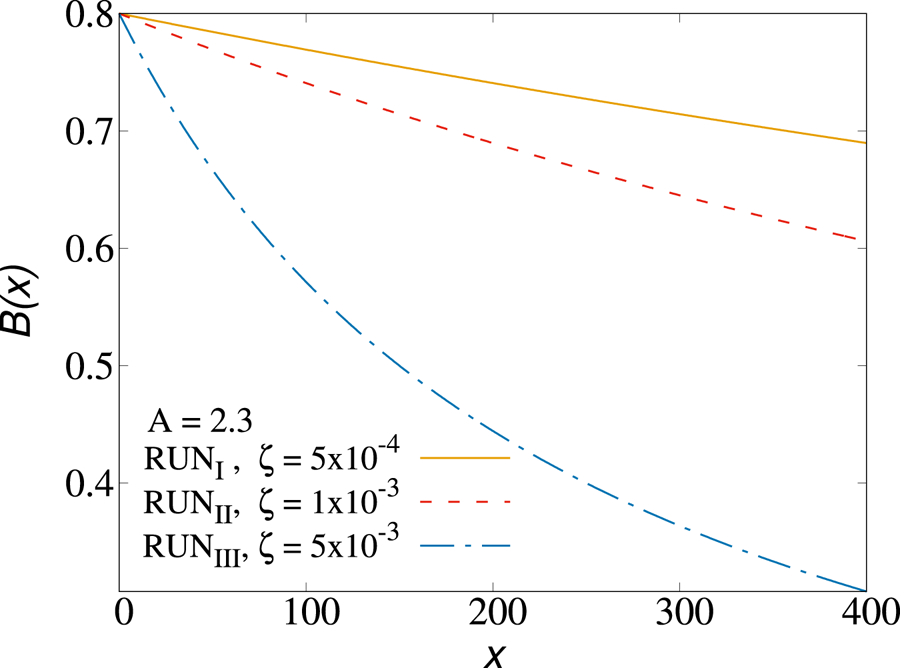
Typical magnetic field profiles for the simulations performed in this work are shown in figure 1.
Magnetic fields profile in RUN$_{\rm I}$ , RUN$_{{\rm II}}$
 , RUN$_{{\rm III}}$
 . As $\zeta$
 increases, the magnetic field drops faster along the radial coordinate(the gradient of $\boldsymbol {B}$
 becomes larger).

The assumption of considering $\boldsymbol {u}_E$ as the dominant contribution to the plasma motion (drift approximation) allows us to write the vorticity $\varOmega$
 as the curl of the electric drift in the plane perpendicular to $\boldsymbol {B}$
 , i.e. $\varOmega = \hat {\boldsymbol {z}} \boldsymbol {\cdot } (\boldsymbol {\nabla } \times {\boldsymbol {u}_E}) = {\nabla ^2{\phi }}/{B}$
 (Militello et al. Reference Militello, Fundamenski, Naulin and Nielsen2012). Equation (2.3) has been therefore obtained by considering the difference between the continuity equation for ions and electrons and making use of the above assumptions.
2.1. The numerical code
We developed an algorithm that solves (2.1)–(2.4) by using a combination of finite differences and Runge–Kutta techniques. The 2-D code solves the equation in the ($x, y$ ) plane assuming periodicity in the $y$
 direction. We used classical, second-order, centred finite differences for the spatial differentiation and second-order Runge–Kutta for the temporal evolution of the system. The code adopts a combination of finite differences and spectral methods to solve the Poisson equation, as commonly done in systems with a periodic direction (see below).
The domain consists of a rectangular box of size $L_x \times L_y$ and a cell-centred grid with $N_x$
 equidistant points in the $x$
 -direction and $N_y$
 equidistant points in the $y$
 -direction. In particular, we used a box of $N_x \times N_y = 512 \times 256$
 mesh points. The physical region of our simulation domain corresponds to a small rectangle, perpendicular to the mean field, at the boundary of the LCMS. It includes the outer region of the plasma column, in our domain at $x = 0$
 , extending to the SOL and the near-wall region of a typical fusion device (at $x = L_x$
 ). We normalized these directions to the hybrid gyration radius $\rho _s=c_s/\omega _{ci}$
 , and in these normalized units, $L_x = 400$
 and $L_y = 200$
 . The radial position corresponding to the LCMS is located at $x_0 = 100$
 .
We applied the following boundary conditions in the radial direction $x$ . At $x = 0$
 (the inner boundary) $\varOmega = 0$
 , and for the gradients ${\partial n}/{\partial x} = {\partial T}/{\partial x} = {\partial \varOmega }/{\partial x} = {\partial \phi }/{\partial x} = 0$
 . For the outer boundary, at $x=L_x$
 , we chose $\phi _0 = \varOmega = 0$
 , $n=T=1$
 and again null gradients (Garcia et al. Reference Garcia, Naulin, Nielsen and Rasmussen2005). The quantity $\phi _0$
 represents the poloidal average at $L_x$
 of the potential.
The initial profile of the density has been chosen as a function with a steep gradient along the radial coordinate corresponding to the LCMS, which analytical form corresponds to $n(x, y) = n_i - \Delta n( 1 + \tanh { (x-x_0)/12 } )$ . Here, $n_i$
 is the value of the density at the inner boundary of the simulation domain, and $\Delta n$
 is a parameter used to modulate the shape of the function, its ‘jump’, so that it always satisfies the outer boundary conditions. In our model, we considered equal initial profiles for both density and temperature. Therefore, we defined the parameter $A$
 as $A = n_i = T_i$
 and $\Delta A = \Delta n = \Delta T$
 .
Because of periodicity, $\phi$ and $\varOmega$
 can be expressed in terms of the Fourier basis as $\phi (x,y)=\sum _{n=1}^{N_y} \hat {\phi }(x)\exp ({{\rm i} n 2{\rm \pi} /L_y y})=\sum _{n=1}^{N_y} \hat {\phi }(x)\exp ({{\rm i} n k_y y})$
 and $\varOmega (x,y)=\sum _{n=1}^{N_y} \hat {\varOmega }(x)\exp ({{\rm i} n k_y y})$
 (here, we suppressed the time dependency, for simplicity). Then, by employing a centred finite difference scheme for the second $x$
 -derivative of $\phi$
 , from (2.4), one gets the following equation at the $j$
 th grid point in the $x$
 -direction:

By considering the $x$ -boundary conditions discussed above, the previous equation can be written in the form of a linear tridiagonal system for the unknown coefficients $\hat {\phi }(x_j), j=1,\ldots,N_x$
 . This linear system can be solved through standard linear algebra routines (Press et al. Reference Press, Teukolsky, Vetterling and Flannery1996). Finally, the inverse Fourier transform in $y$
 returns the values of $\phi (x_j,y_l)$
 at all grid points in the numerical 2-D box.
Regarding the shape of the magnetic field, it was important to set the parameters $\epsilon$ and $\zeta$
 . Following the literature, their values are usually small, and we set $\epsilon = 0.25$
 . Since we want to study a toroidal system characterized by a radial gradient of the main magnetic field, we have always assumed a non-null curvature parameter $\zeta$
 . With this setting, any small perturbation suddenly generates instabilities and turbulence. These instabilities, indeed, are suppressed for $\zeta = 0$
 , because there is no magnetic gradient that causes the vertical polarization, and hence a radial electric drift. Without this gradient there is no triggering of interchange instability mechanism. This scenario was confirmed by performing a test simulation (not shown here) in which we set $\zeta = 0$
 .
The collisional coefficients $\nu _n = \nu _T = \nu _\varOmega$ are set to a very low number (${\sim }10^{-2}$
 ), in order to resolve well the structures and to dissipate artificial small-scale fluctuations. In the expression of the linear damping, (2.5), two other parameters have to be defined. In particular, we used $\lambda = 1.6 \times 10^{-4}$
 and $\delta = 1$
 . The parameters $\zeta$
 and $\nu$
 are varied for each run, as described in the next section.
The large-scale plasma profile cannot be described self-consistently in the framework of our simplified (reduced) Braginskii model. For $x< x_0$ , the closed field line region, we therefore maintain constant the mean large-scale profiles, assuming that these would vary on time scales much larger than the typical turbulence dynamical times. In our numerical simulations, a steady-state regime of transport is ensured by maintaining constant time density and temperature poloidal profiles. In this regard, we developed a new driving technique based on an averaging method: we forced the initial poloidal average of the density and temperature fields to remain constant within the LCMS region. The poloidal average of any field is defined as the spatial average over the periodic direction, namely $\langle f \rangle (x) = ({1}/{L_y})\int f(x,y') \,{{\rm d} y}'$
 . In our model, at each time step, we subtracted the poloidal averages of the plasma density and temperature, replacing them with the initial profiles. This procedure was applied only in the first part of the domain, for $x < x_0$
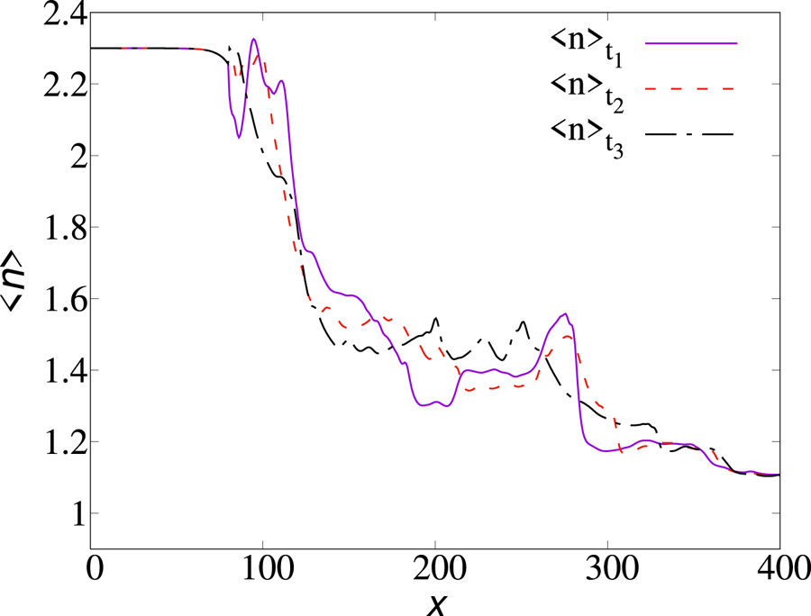
 . The method is very efficient and allows us to achieve a stationary configuration of emission/absorption. This novel technique, different from the previous modelling of edge turbulence, is based on maintaining a constant poloidal inner profile. We named this novel forcing procedure the average freezing driving (AFD). In figure 2 we report the behaviour of the poloidal average of the density as a function of time, during a turbulent steady state. A similar approach, applied to other geometries, has been found to give very stable, statistically steady-state simulations of SOL turbulence (Servidio et al. Reference Servidio, Primavera, Carbone, Noullez and Rypdal2008).
Poloidally averaged density at three different times. The initial mean profile remains fixed in the inner region of the simulation domain (RUN$_{{\rm II}}$ ).

3. Numerical results
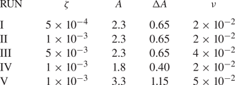
The numerical model discussed in the previous section is suited to reproducing the turbulent dynamics of the outer region of fusion devices. Here, we report the main results of our numerical simulations. We performed a campaign of runs, summarized in table 1, where we vary mainly two important parameters, namely (i) the inner boundary values of the density and the temperature, $n_i$ and $T_i$
 , and (ii) the magnetic shear parameter $\zeta$
 . These changes allow us to inspect different turbulent regimes and to study the variations in the dynamics of blobs. For RUN$_{{\rm II}}$
 , chosen as a reference simulation, we have imposed an amplitude $A\equiv n_i=T_i$
 of 2.3 and $\zeta = 10^{-3}$
 . The latter values are in agreement with previous works of the reduced Braginskii model (Garcia et al. Reference Garcia, Naulin, Nielsen and Rasmussen2004, Reference Garcia, Naulin, Nielsen and Rasmussen2005, Reference Garcia, Horacek, Pitts, Nielsen, Fundamenski, Naulin and Rasmussen2007; Militello et al. Reference Militello, Fundamenski, Naulin and Nielsen2012).
Parameters used in the different runs. Here, ‘RUN’ indicates the simulation label, $\zeta$ the magnetic shear parameter, $A$
 the edge fixed density, $\Delta A$
 the relative density jump, $\nu$
 the viscous coefficients. We used a time step sufficiently small, with $\Delta t = 0.05$
 , written every $100$
 unit times. For the temperature driving, we set the same jump conditions as for the density ($A\equiv n_i=T_i$
 ). The particle injection time $T_{0p}$
 is set at 2500, while the total number of particles is $N=10\,000$
 .

We analysed the outcome of the simulations via classical statistical analysis of turbulence, using both the Eulerian and Lagrangian approaches, as described in the next subsections.
3.1. The Eulerian approach
In order to characterize the dynamics of SOL turbulent plasmas, it is important to define some relevant global quantities. The radial profile of any field, denoted hereafter by a ‘zero’ subscript, is defined as its spatial average over the periodic direction $y$ (as done for the driving technique.) We can define the density and the poloidal flux profiles as $n_0(x,t) = ({1}/{L_y}) \int ^{L_y}_0 n(x,y,t)\,{{\rm d} y}$
 and $\nu _0(x,t) = ({1}/{L_y} )\int ^{L_y}_0 ({\partial \phi }/{\partial x})\,{{\rm d} y}$
 (Garcia Reference Garcia2001). The deviation from the mean profile of any field is identified as the spatial fluctuation and it is indicated by a tilde, i.e. $\tilde {n}(x,y,t) = n(x,y,t)-n_0(x,t)$
 . Note that, because of the driving at $x< x_0$
 , both the poloidal averages of particle density and temperature are constant in time in this inner region. This is an advantage of the AFD, which guarantees stable profiles in time.
To characterize the turbulent state of the system in the outer layer, we studied the evolution in time of the kinetic energy, considering its two components

that is, the kinetic energy in the fluctuating motions and the sheared poloidal flows, respectively. Following Garcia et al. (Reference Garcia, Bian, Paulsen, Benkadda and Rypdal2003), the evolution of these integrals is given by some straightforward manipulations of (2.3) and (3.1a,b), leading to


where $\tilde {u}_x$ and $\tilde {u}_y$
 are the radial and poloidal components of the electric drift $\boldsymbol {u}_E$
 , respectively. The first term of (3.2) corresponds to the fluctuating motion change due to the radially advective transport of thermal energy. The second (which appears also in (3.3)) represents the conservative transfer of kinetic energy from fluctuating motion to the sheared flow (i.e. kinetic energy may be transferred between the convective cells and sheared poloidal flows by a radial inhomogeneity in the off-diagonal components of the averaged Reynolds stress tensor). The last term, present in both equations, $\varLambda _\varOmega = \nu _\varOmega \nabla ^2 \varOmega - \sigma _{\varOmega }(x) \varOmega$
 , represents the diffusive term and the linear damping due to collisions and particle transport. It corresponds to the right-hand side of (2.3). To summarize, the energy transfer rates from thermal energy to the fluctuating motion, and from fluctuating to the sheared flows, can be defined, respectively, as

These fluxes are crucial for the characterization of turbulent transport, as we shall see in the following.
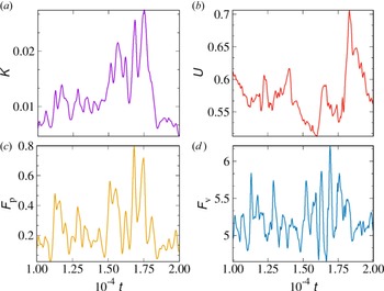
The energies in (3.1a,b) and the fluxes in (3.4a,b) are highly representative of the system dynamics. Hereafter, we show the results for the main RUN$_{{\rm II}}$ . The relation between all the above global quantities is better represented in figure 3, where we focused on a single ‘burst event’. In correspondence with blob ejection, there is a rapid growth of the energy transfer rate $F_p$
 since the available source of free energy, contained in the mean pressure gradient, is converted into $K$
 . Then, after a short time, there is a rapid decrease of the latter in favour of the sheared poloidal flow. A peak in the quantity $F_v$
 is at the same time observed, although there is a small time shift with the burst in $U$
 . Overall, these peaks and correspondences are only qualitative, since they emerge from high-level turbulent fluctuations. Both the trend of the kinetic energy and that of the energy transfer rate suggest that the SOL is characterized by the alternation of blob ejection moments and quiet periods.
Kinetic energy and energy transfer rate in a single burst event. Panels represent (a) kinetic energy in the fluctuating motion $K$ , (b) the sheared poloidal flow $U$
 , (c) the energy transfer rate from thermal energy to the fluctuating motion $F_p$
 and (d) the transfer rate from fluctuating to sheared flows $F_v$
 .

Generally, the evolution in time of the kinetic energy of the fluctuating motions is characterized by irregular oscillations with pronounced bursts. This is a manifestation of intermittent, bursty turbulence, typically observed at the edge of many tokamak devices. During such burst events, the formation of blobs takes place. Every time that this fluctuation level is sufficiently large, there is a rapid growth of the energy in the sheared poloidal flows $U$ , followed by a suppressed level of $K$
 . Such a dynamics is the consequence of the exchange of kinetic energy from the fluctuating motion to the sheared flows, as can be evinced from (3.2)–(3.3).
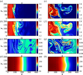
The difference between an emission moment (right) and a quiet period (left) is reported in figure 4 for density, temperature, vorticity and potential, from top to bottom, respectively. In the quiet regime, the plasma is quite homogeneous and isothermal and almost no fluctuations can be observed in the SOL region. There are plumes in the particle density and temperature fields. At the time of a burst event (e–h), it is evident that prominent structures develop in the SOL. During such a burst event, an accumulation of particle density and heat is clearly evident. This ejection is localized in the region of the LCMS, in the SOL, at $x>x_{0}$ .
Comparison of the spatial structure of particle density, temperature, vorticity and potential during a quiet period, (a–d), and during a burst event, (e–h).

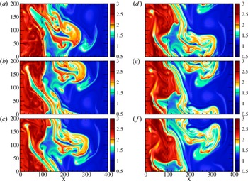
During a burst event, it is possible to observe the formation of a blob by following the evolution over time of particle density, as can be seen from figure 5. These plots show the rapid development of a structure from the inner region to the outer part of the domain, i.e. towards the open wall. During the emission, the main vortex can also merge with and eat small neighbouring fluctuations.
Spatial evolution of particle density over time, in sequence from (a–f), showing a blob emission from the edge of the plasma column and its propagation towards the outer boundary.

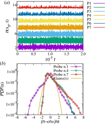
Another useful Eulerian analysis that can help to understand the propagation in space and time of turbulent structures is the analysis of macroscopic variables such as the density at selected regions of the numerical domain (to mimic probe measurements in the SOL). We measured the density and its probability distribution function (p.d.f.) at different points (probes) of the simulation domain. These are 7 probes equally spaced, numbered going from left to right of the domain (so the first probe is situated in the plasma edge region, while the last one is near the wall). These equally spaced probes start at $x_1= 64$ , following at $x_j = j \delta$
 , with $j = 2,\ldots, 7$
 with separation $\delta =64$
 .
Panel $(a)$ of figure 6 represents the change in time of the density at different points of the domain. The signal is stronger at the first probes, because of the higher concentration of density in the inner region. Progressively, the amplitude decreases near the wall, at probe $P_7$
 . We can see that some events are correlated. These effects are due to the turbulent transport and reveal that blobs structures are moving radially toward the wall. The particle density at the probes within the edge region, $P_1$
 and $P_2$
 , shows chaotic oscillations which appear symmetric concerning the mean value, while all other probe signals reveal predominantly positive fluctuations (higher skewness), as highlighted also from the p.d.f. analysis.
(a) Temporal evolution of the particle density measured by the different probes $P_j$ . Note that the signal has been shifted in the $y$
 -axis to compare, on the same plot, all the measurements; (b) The p.d.f. of the particle density signals, compared for three different probes.

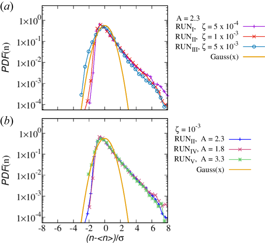
In figure 6(b), we report the p.d.f. of the particle density, at three different probes. The presence of intermittent fluctuations causes a departure of the p.d.f. from the normal distribution, manifesting very high exponential tails (Antar et al. Reference Antar, Krasheninnikov, Devynck, Doerner, Hollmann, Boedo, Luckhardt and Conn2001b; Garcia et al. Reference Garcia, Bian, Paulsen, Benkadda and Rypdal2003; Sattin et al. Reference Sattin, Vianello, Valisa, Antoni and Serianni2005; Killer et al. Reference Killer, Narbutt and Grulke2021; Tatali et al. Reference Tatali, Serre, Tamain, Galassi, Ghendrih, Nespoli, Bufferand, Cartier-Michaud and Ciraolo2021). This is typical of intermittent, extraordinary events. As we can see, at the first probe which is located within the plasma edge, the ${\rm p.d.f.}(n)$ has a nearly symmetric, super-Gaussian shape. At larger distances from the LCMS, due to the intermittent nature of turbulence, it gradually develops higher tails, skewed in the outward direction. This skewness and kurtosis of the distribution is commonly observed in SOL of fusion devices and reflects the high probability of extreme events, as largely investigated in the literature (Antar et al. Reference Antar, Counsell, Yu, Labombard and Devynck2003; van Milligen et al. Reference van Milligen, Sánchez, Carreras, Lynch, LaBombard, Pedrosa, Hidalgo, Gonçalves and Balbín2005; Xu et al. Reference Xu, Jachmich and Weynants2005; Kamataki et al. Reference Kamataki, Itoh, Inagaki, Arakawa, Nagashima, Yamada, Yagi, Fujisawa and Itoh2010).
At this point, we changed the simulation settings to explore the parameter space. By changing $\zeta$ and $A$
 , we analysed different turbulent regimes and compared all the simulations by evaluating their power spectra and the p.d.f.s of the particle density. For the power spectra, we Fourier transformed the density field $n(x,y,t)$
 along the periodic direction, computed the energy spectrum $E(x, k_y, t)=|\tilde {n}(x, k_y, t)|^2$
 ($\tilde {n}$
 being the Fourier coefficient) and finally obtained the spectrum from an ensemble average both in time and space (in the region $x>x_{0}$
 ).
In RUN$_{\rm I}$ , RUN$_{{\rm II}}$
 and RUN$_{{\rm III}}$
 we have increased progressively the value of $\zeta$
 . Since this parameter governs the variation along the radial coordinate of the magnetic field, we have effectively increased the gradient of $\boldsymbol {B}$
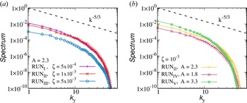
 , as can be evinced from figure 1. In figure 7(a) we compare the averaged spectra of the plasma density $n$
 , as a function of the poloidal mode $k_y$
 , for this campaign of runs. The turbulent spectrum progressively decreases from RUN$_{\rm I}$
 to RUN$_{{\rm III}}$
 . The spectra all manifest a power-law scaling, consistent with a fluid-like turbulent cascade (Kolmogorov Reference Kolmogorov1941a, Reference Kolmogorovb). We report also the Kolmogorov scaling law as a reference. Even if the scaling is consistent from one run to another, the level of turbulence decreases. This trend reveals that an increase in the value of $\zeta$
 leads to more stable configurations, while the system characterized by a small value of $\zeta$
 is affected by a stronger turbulent transport. The suppression of turbulent transport is also evident in the p.d.f.s in figure 8(a): the low-$\zeta$
 cases are more intermittent.
(a) Comparison between the average energy spectrum of RUN$_{\rm I}$ , RUN$_{{\rm II}}$
 , and RUN$_{{\rm III}}$
 . The energy spectrum decreases as the $\zeta$
 value increases, revealing a more stable configuration in the RUN$_{{\rm III}}$
 , which is characterized by a higher value of $\zeta$
 ; (b) Comparison between the average energy spectrum of RUN$_{{\rm II}}$
 , RUN$_{{\rm IV}}$
 , and RUN$_{{\rm V}}$
 . In this case, the energy spectrum decreases in the presence of a smaller pressure gradient, reflecting the hypothesis that a higher gradient of density injects more turbulence into the system.

(a) Comparison of the p.d.f. of particle density between RUN$_{\rm I}$ , RUN$_{{\rm II}}$
 , and RUN$_{{\rm III}}$
 . More pronounced tails are present in the RUN$_{\rm I}$
 and RUN$_{{\rm II}}$
 rather than in the RUN$_{{\rm III}}$
 , indicating more intermittency in the former cases; (b) Comparison of the p.d.f. of particle density between RUN$_{{\rm II}}$
 , RUN$_{{\rm IV}}$
 , and RUN$_{{\rm V}}$
 . The latter p.d.f.s are quite similar, revealing that density and temperature gradients do not influence too much the nature of the intermittent transport.

RUN$_{{\rm II}}$ , RUN$_{{\rm IV}}$
 and RUN$_{{\rm V}}$
 are characterized by different values of the initial density and temperature jump $A$
 , as described in the table. Changing the value of these quantities at the inner boundary of the domain corresponds to a variation of the gradient of pressure that, as a consequence of the inhomogeneity of the magnetic field $\boldsymbol {B}$
 , drives instabilities. From the spectra in figure 7(b) it is clear that higher density and temperature gradients (higher $\Delta A$
 ) cause more turbulent activity. The intermittent behaviour does not seem to be affected so much by the change of $A$
 , as can be seen from the p.d.f.s in figure 8(b). This picture confirms that the available source of free energy, driving the convective motions, is contained in the mean pressure gradient. An increase in the free energy leads to an increase in the fluctuating motion and, consequently, to a higher (radial) turbulent transport.
3.2. The Lagrangian approach
In the second part of our analysis, in order to better understand the diffusion of fluid elements in the SOL region and characterize the transport dynamics, a new technique is investigated, based on the Lagrangian approach. We followed in time the motion of fluid tracers in the drift approximation, integrating the trajectory of the plasma element in the numerical domain. In practice, we solved particle integration in our code, following the journey of plasma elements from the central part of the LCMS toward the colder, empty regions at the wall. We solved the fluid equations of motion in which we considered only the major contributions of the cross-field fluid drift – the electric and the diamagnetic drifts.
The equation of motion for the fluid tracers has been derived by using the same Braginskii approximation of our model: we neglected the ion dynamics, concentrating only on the motion of the electrons, and neglected the inertial term in the cross-field drift. The drift velocity then is simply

Plasma fluid elements, therefore, move with the above velocity, at each time, by obeying to $\dot {\boldsymbol {x}} = \boldsymbol {u_\perp }$ . We integrated the trajectories of fluid particles that follow passively the flow. In this regard, we upgraded the numerical code with this Lagrangian tracing technique where the fields have been continuously supplied by the time-varying simulation, and by obtaining the velocity (3.5) at each particle position via a bilinear interpolation algorithm (second order in space).
At the beginning (or at the earlier stages) of each simulation, we placed all the Lagrangian tracers at the LCMS ($x_0$ ), but with different (random) poloidal positions $y$
 . We considered the following boundary condition for the tracers: if an element reaches the radial boundary, we removed it from the domain (this is because we are interested in particles within the SOL region); in the poloidal direction, instead, we considered periodic boundaries. The parameters of the Lagrangian integration are summarized in table 1, and their initial motion is represented in figure 9. We show the evolution in time of the trajectories for just 10 fluid elements, to avoid overcrowding. In this figure, one can see how, from the radial position corresponding to the LCMS, elements start their erratic trip in the simulation domain under the effect of turbulence. Some of them are absorbed by the left part of the wall, namely inside the device. Some of them are lost from the outer SOL (right side).
Examples of trajectories of the fluid elements, for RUN$_{{\rm II}}$ , starting from the initial position at $x_0$
 (here highlighted by a black vertical line). Only early times of such trajectories, for a limited sample, are reported.

To perform a statistical analysis of the turbulent diffusion mechanism, we considered a large sample of fluid elements, $N = 10\,000$ , and calculated their displacement from the initial position $\Delta x(t)= x(t)-x_0$
 , along the $x$
 axis. Note that, with this set-up, the maximum value of the displacement is $\Delta x_{\max } = 300$
 . We verified the convergence of the statistics presented below by increasing systematically the number of particles, as reported later in this section. We noticed that plasma elements in the SOL region experience an irregular random walk.
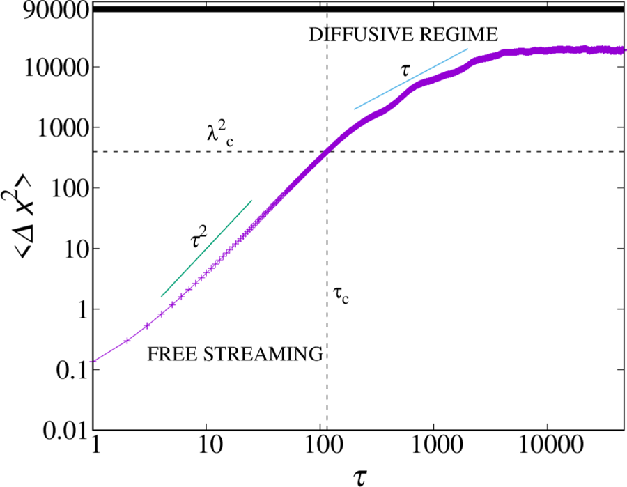
To make contact with classical diffusion theories, we evaluated the mean square displacement (MSD) of the radial positions $\langle \Delta x^2 \rangle$ , where $\langle \bullet \rangle$
 represents an ensemble over all the particles. In figure 10, we reported the MSD as a function of time. The behaviour of the MSD is quite interesting, given the fact that we are in a small, finite-size system. In the initial stage of their journey, the particles experience a behaviour consistent with $\tau ^2$
 , typical of free-streaming motion (Taylor Reference Taylor1921; Taylor & McNamara Reference Taylor and McNamara1971; Huang et al. Reference Huang, Chavez, Taute, Lukić, Jeney, Raizen and Florin2011; Pusey Reference Pusey2011). Here, $\tau$
 is simply the difference between $t$
 and the injection time $T_{0p}$
 (see table 1). After the above initial transient, the curve suggests a diffusive behaviour, $\langle \Delta x^2\rangle \sim \tau$
 . As in typical plasma turbulence (Pecora et al. Reference Pecora, Servidio, Greco, Matthaeus, Burgess, Haynes, Carbone and Veltri2018), this regime starts when the displacement becomes of the order of the correlation length of turbulence $\lambda _c$
 . The latter corresponds to the typical size of the largest energy-containing eddies, namely the size of the blobs. For the above simulations, we estimated this length to be, qualitatively, $\lambda _c \sim 20$
 . The regime of the diffusive transient starts therefore at a characteristic correlation time $\tau _c$
 , highlighted in the figure with a vertical line. At later times, contrary to unbounded problems of diffusion, the behaviour is influenced by the system size, and the large-scale diffusive regime is lost. At these large times, most of the particles abandoned the domain, either because they are absorbed by the inner boundary or because they are lost at the outer wall.
Temporal evolution of the mean square displacement of the fluid elements, in a double logarithmic scale, for RUN$_{{\rm II}}$ . The horizontal (dashed) line represents the square of the correlation length $\lambda _c$
 , namely the average size of the blobs. The characteristic decorrelation time is reported with a vertical dashed line. The thick (black) line represents the maximum allowed MSD, $\Delta x_{\max }^2$
 .

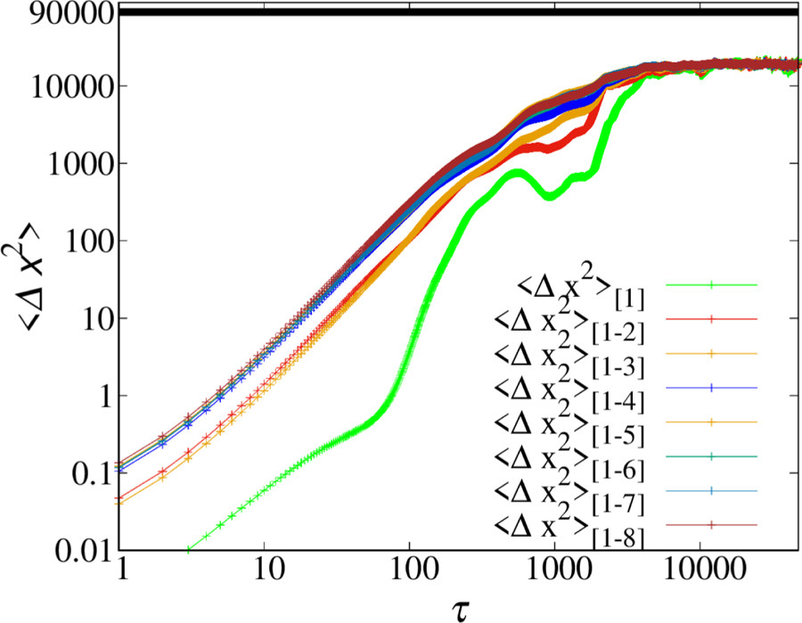
To further confirm this diffusive behaviour, we computed the diffusion coefficient, but first, we checked the convergence of our results by increasing systematically the statistics. We divided the simulation times into subdomains. In particular, we divided the particle integration into eight, smaller, subsequent shots, each of which lasts $5\times 10^{4}$ computational times. At each particle restart, we set all the fluid elements at the initial position ($x_0 = 100$
 ) and we studied how the diffusion changes over time. In figure 11 we show the temporal convergence of the MSD: ‘$\langle \Delta x^2\rangle _{[1]}$
 ’ refers to the MSD of the first part of the simulation, the second, $\langle \Delta x^2\rangle _{[1-2]}$
 , refers to the average of the first and second part of RUN-II, and so on. We continued to enlarge the statistics until we comprehended all the eight time subdomains. We can observe that the curves progressively increase, until they collapse, suggesting a clear convergence of the statistics (note that the convergence is achieved already with an average on just six subsets).
Convergence of the statistical analysis, for RUN$_{{\rm II}}$ . Other runs have similar behaviours.

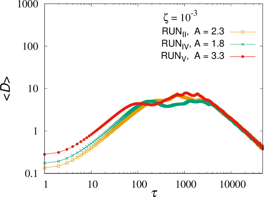
At this point, the diffusion coefficient can be computed as $D \sim \langle \Delta x^2\rangle /(2 \tau )$ , for each average shown in figure 11. Similar behaviour has been found for different runs (not shown here). We compared the diffusion coefficient, averaged over all the datasets, for the runs where we had a strong enhancement of turbulence, namely by comparing RUN$_{{\rm II}}$
 , RUN$_{{\rm IV}}$
 and RUN$_{{\rm V}}$
 . In figure 12 one can see that diffusion is effectively higher for the run with stronger turbulence, namely the case where the density and temperature driving is more intense ($A=3.3$
 ). This preliminary analysis of the diffusion process further confirms that turbulence enhances particle diffusion, even in such a simplified Braginskii model of the SOL.
Comparison of the diffusion coefficients (in a double logarithmic scale) between RUN$_{{\rm II}}$ , RUN$_{{\rm IV}}$
 and RUN$_{\rm V}$
 .

4. Conclusions
A 2-D simplified model has been adopted to study the turbulent dynamics in the region of the SOL. We showed how the numerical model, based on the reduced Braginskii equations, can describe the formation and the evolution over time of blob structures. We studied this complex dynamics by varying the ambient conditions of the plasma, and by using both classical Eulerian analysis and the Lagrangian approach. The novelty of our work consists of (i) a detailed and systematic study of turbulence by varying the plasma jump conditions in the edge laboratory plasmas, and (ii) an analysis of the fluid elements diffusion by using a Braginskii model. Moreover, our work has validity regarding the numerical methods, since we propose a novel driving technique for edge turbulence.
We conducted a simulation campaign where we varied the magnetic shear intensity and the level of injected turbulence. We proposed a new technique for driving bursty turbulence based on the freezing of the main plasma profiles in the inner region of the SOL. As in previous works, we observed an intermittent character of turbulence, where the latter is composed of blobs of plasma that propagate outward, from the LCMS toward the walls. The radial flux is dominated by mushroom-like blobs that move with the $E\times B$ drift. The statistical analysis of the flux, as measured by single probes in the domain, is in agreement with experimental observations, manifesting highly non-Gaussian p.d.f., characterized by intermittent, extreme events.
By varying the simulation parameters, in a steady-state regime of driven turbulence, we observed that the turbulence level is higher for smaller coefficients $\zeta$ of the Braginskii model. Similarly, the turbulence intensity increases with larger density and temperature jumps, going from the internal to the outer region.
In the second part of the work, we inspected the diffusive properties of the plasma by integrating fluid trajectories, under the fluid-drift approximation. Following a large sample of elements, we observed a diffusive transient, for a length scale larger than the typical blob size.
This numerical campaign presents several results, giving a qualitative picture of how turbulence statistics are affected by changing the radial scale length of the magnetic field and the pressure. The work is relevant for the comprehension of the turbulent transport at the edges of tokamak devices. Future studies will be devoted to the modelling of larger domains with higher resolutions. A more detailed theoretical investigation of the diffusive process will be presented together with an analysis of the effect of neutrals on the dynamics of the system.
Acknowledgements
We would like to acknowledge W. H. Matthaeus for the useful discussion in the early stages of this paper.
Editor Francesco Califano thanks the referees for their advice in evaluating this article.
Funding
The work and simulations have been supported by ‘Progetto STAR 2-PIR01 00008’ (Italian Ministry of University and Research).
Declaration of interests
The authors report no conflict of interest.